Form factors for semi-leptonic $B$ decays

Abstract:

Semi-leptonic $B$ decays provide promising channels to test the Standard Model, search for signs of new physics, or determine fundamental parameters like CKM matrix elements. We present an update on our calculation of short distance contributions to GIM suppressed rare $B$ decays focusing in particular on $B_{s}\to\phi\ell^{+}\ell^{-}$ decays. Furthermore we show first results for our calculation of $B_{(s)}\to D_{(s)}^{(*)}\ell\nu$ semi-leptonic decays involving $b\to c$ transitions.
Our calculations are based on RBC-UKQCD’s 2+1 flavor domain-wall fermion and Iwasaki gauge field configurations featuring three lattice spacings in the range $1.73$ GeV $\leq a^{-1}\leq 2.77$ GeV and pion masses down to the physical value. We calculate the form factors by simulating $b$-quarks using the relativistic heavy quark action, create light $u/d$ and $s$ quarks with standard domain-wall kernel, and use optimised Möbius domain-wall fermions for charm quarks.

darkgreenrgb0,.6,0

1 Introduction

Semi-leptonic $B_{(s)}$ decays are receiving considerable attention both experimentally and theoretically. They allow to determine fundamental parameters of the Standard Model (SM), like Cabbibo-Kobayashi-Maskawa (CKM) matrix elements providing constraints on the SM in searches for new physics. At tree-level in the SM, only charged flavor changing currents occur and transitions of bottom quarks to charm or up quarks are suppressed by the small size of the corresponding CKM matrix elements. Those decays are depicted by sketch a) in Fig. 1. Transitions of bottom quarks to down or strange quarks may occur in the SM only at loop level (see sketches b) and c) in Fig. 1) and the corresponding flavor changing neutral currents (FCNC) are further suppressed due to the Glashow-Iliopoulos-Maiani (GIM) mechanism [1]. Since in the SM these transitions are highly suppressed, they are good candidates to search for new physics. Anomalies have been reported comparing SM predictions and experimental results, e.g., for angular observables [2], branching fractions [3], and the ratio $R_{K}$ [4], but are also observed in charged tree-level $b\to c$ transitions see e.g. [5, 6, 7, 8].

Figure 1: Diagrams sketching the calculation of non-perturbative, short distance contributions to semi-leptonic decays: a) charged tree-level decay $\big{(}$e.g., $B\to\pi\ell\nu$, $B_{s}\to K\ell\nu$, or $B_{(s)}\to D_{(s)}\ell\nu\big{)}$, b) and c) loop-level decays with flavor changing neutral currents $\big{(}$e.g., $B_{s}\to\phi\ell^{+}\ell^{-}\big{)}$. The short distance contributions are indicated by the gray shading and implemented as point-like operators.

Besides experimental measurements, theoretical determinations of form factors are needed to test the SM. After carrying out an operator product expansion (OPE), we conventionally classify terms into “short” and “long” distance contributions. In the following we solely focus on the computation of short distance effects as one ingredient to better constrain the SM. On the theory side the uncertainties of these short distance contributions arise predominately from hadronic effects. Using lattice quantum chromodynamics (QCD) techniques, we have set-up a program to determine form factors for semi-leptonic $B_{(s)}$ decays. This program started by calculating semi-leptonic form factors for $B\to\pi\ell\nu$ and $B_{s}\to K\ell\nu$ [9] and last year we reported on generalizing our code to additionally compute GIM suppressed decays with hadronic pseudoscalar or vector final states [10]. Here we will present updates on our calculation involving FCNC and, furthermore, present first results for bottom quarks transitioning to charm quarks. When combined with experimental measurements, $B\to D^{(*)}\ell\nu$ form factors allow to determine the CKM matrix element $|V_{cb}|$ but will also allow to compute ratios of branching fractions $R_{D}^{(*)}$

$$R_{D^{(*)}}=\frac{{\cal B}(D\to D^{(*)}\tau\nu_{\tau})}{{\cal B}(D\to D^{(*)}\ell\nu_{\ell})},\qquad\text{with}\quad\ell=e,\,\mu.$$ (1)

Only very recently the long-standing $2-3\sigma$ discrepancy between inclusive and exclusive determinations of $|V_{cb}|$ seems to disappear [11]. The tension between SM predictions and experimental findings for $R_{D}$ and $R_{D^{*}}$ [5, 6, 7, 8] are however independent of $|V_{cb}|$ and warrant further investigations. Independent lattice determinations of $B\to D^{(*)}\ell\nu$ semi-leptonic form factors will help to do so.

The remainder of this article is organized as follows: In the next Section we present the set-up of our computation and give details on the actions and ensembles used in our simulations. In Section 3 we report on our progress to compute rare semi-leptonic $B$-decays mediated by FCNCs. Due to the limited space, we will focus here on $B_{s}\to\phi\ell^{+}\ell^{-}$ decays. In Section 4 we present our setup for $B_{(s)}\to D_{(s)}^{(*)}\ell\nu$ decays with charm quarks discretized as DWF. Finally we give a brief outlook and conclude.

2 Computational set-up

		$a^{-1}$				$M_{\pi}$		# time
$L^{3}\times T$	$L_{s}$	[GeV]	$am_{l}$	$am_{h}$	$am_{s}^{\text{phys}}$	[MeV]	# configs	sources
$24^{3}\times 64$	16	1.785(5)	0.005	0.040	0.03224(18)	340	1636	1
$24^{3}\times 64$	16	1.785(5)	0.010	0.040	0.03224(18)	434	1419	1
$32^{3}\times 64$	16	2.383(9)	0.004	0.030	0.02477(18)	302	628	2
$32^{3}\times 64$	16	2.383(9)	0.006	0.030	0.02477(18)	360	889	2
$32^{3}\times 64$	16	2.383(9)	0.008	0.030	0.02477(18)	411	544	2
$48^{3}\times 96$	24	1.730(4)	0.00078	0.0362	0.03580(16)	139	40	162
$48^{3}\times 96$	12	2.77(1)0	0.002144	0.02144	0.02132(17)	234	50	24

Table 1: Overview of the used gauge field ensembles. The ensembles were generated by the RBC and UKQCD collaborations [12, 13, 14, 15] using 2+1 flavor domain-wall fermions and Iwasaki gauge actions. The domain-wall height for light and strange quarks is $M_{5}=1.8$. The $24^{3}$ and $32^{3}$ ensembles are generated using the Shamir domain-wall kernel [16, 17], while $48^{3}$ ensembles use the Möbius kernel with $\alpha=2$ [18]. Values for the inverse lattice spacing and the quark and meson masses are taken from the refined analysis [14] and updated to include the finer $a^{-1}=2.77$ GeV ensemble [15]. The light sea-quark mass is labeled $am_{l}$, the heavy sea-quark mass $am_{h}$, and $am_{s}^{\text{phys}}$ is the mass of the physical strange quark mass. The valence strange quark masses used in our simulations on $24^{3}$ ($32^{3}$) ensembles are $am_{s}^{\text{sim}}=0.03224\,(0.025)$, while on $48^{3}$ ensembles we used $am_{s}^{\text{sim}}=am_{h}$. Generation of propagators and calculating contractions is ongoing on both $48^{3}$ ensembles.

Our simulations are based on RBC-UKQCD’s set of 2+1 flavor gauge field configurations [12, 13, 14, 15] generated with the Iwasaki gauge [19] and the domain-wall fermion action [16, 17, 18]. Currently our measurements have been completed on the five ensembles at inverse lattice spacings of 1.785 and 2.383 GeV featuring unitary pion masses down to $\sim$300 MeV. Work is in progress to include additional data on the new $48^{3}$ ensemble with $a^{-1}=2.77$ GeV and the $48^{3}$ ensemble featuring physical pion masses at $1.730$ GeV. For all ensembles $M_{\pi}\,L$ is greater than 3.8 and the spatial box sizes are at least 2.6 fm. Details of the used configurations as well as the number of gauge field configurations and sources per configuration are summarized in Tab. 1. In order to reduce autocorrelations between lattices, we perform a random 4-vector shift of the gauge field prior to starting our calculation.

In the valence sector we generate light and strange quark propagators using the same domain-wall fermion formulation as has been used in the sea-sector. We simulate the heavy $b$-quarks using the Fermilab [20] or relativistic heavy quark (RHQ) action [21, 22]. The RHQ action is an effective action based on the anisotropic Sheikoleslami-Wohlert action [23] with a special interpretation of its three parameters ensuring that discretization errors are small. For this work we repeated the non-perturbative tuning of the three RHQ parameters following our prescription published in Ref. [24]. Re-tuning the RHQ parameters was triggered by the refined global fit updating the determinations of lattice spacings [14] which enables us to consistently include the newer $48^{3}$ ensembles. Details of the new RHQ parameters will be published in a forthcoming paper.

Our choices for calculating 2-point and 3-point correlation functions on the lattice are guided by our calculation of $B\to\pi\ell\nu$ and $B_{s}\to K\ell\nu$ semi-leptonic form factors [9]. We choose point-sources for the light and strange quarks, but Gaussian smeared sources [25] for the heavy bottom quarks. Since the separation of source and sink is crucial for obtaining a good signal in the 3-point correlators, we carried out a dedicated study checking for the signal of all form factors contributing to rare $B$ decays in [10]. Our previous choices of $t_{\text{sink}}-t_{\text{source}}=20$ for ensembles with $a^{-1}=1.785$ GeV were confirmed. Scaling that value proportional to the lattice spacing we use $t_{\text{sink}}-t_{\text{source}}=26(30)$ for $a^{-1}=2.383$ (2.77) GeV.

Data presented in the following Sections are analyzed using single elimination jackknife re-sampling after first averaging correlators computed with different sources on the same gauge field configuration.

3 Rare $B$ decays with FCNC

The effective Hamiltonian for weak $b\to q\ell^{+}\ell^{-}$ decays (with $q$ a down or a strange quark and $\ell$ an $e,\,\mu,$ or $\tau$ lepton) is given by [26, 27, 28, 29, 30, 31],

$$\mathcal{H}^{b\to q}_{\text{eff}}=-\frac{4G_{F}}{\sqrt{2}}V^{*}_{tq}V_{tb}\sum_{i=1}^{10}\left(C_{i}O_{i}+C^{\prime}_{i}O^{\prime}_{i}\right),$$ (2)

where $V_{tq}^{*}$ and $V_{tb}$ are CKM matrix elements, $O_{i}^{(\prime)}$ are local operators and $C_{i}^{(\prime)}$ their corresponding Wilson coefficients determined in [32, 33, 34]. Primed operators differ from unprimed ones by their chirality and are even further suppressed in the SM. Short distance contributions are dominated by dileptonic operators (corresponding to Fig. 1c)

$$O_{9} =\frac{e^{2}}{16\pi^{2}}\bar{q}\gamma^{\mu}P_{L}b\bar{\ell}\gamma_{\mu}\ell, O_{10}=\frac{e^{2}}{16\pi^{2}}\bar{q}\gamma^{\mu}P_{L}b\bar{\ell}\gamma_{\mu}\gamma_{5}\ell,$$ (3)

and the electromagnetic operator (Fig. 1b)

$$O_{7}=\frac{m_{b}e}{16\pi^{2}}\bar{q}\sigma^{\mu\nu}P_{R}bF_{\mu\nu}.$$ (4)

In Equations (3) and (4) the lepton is denoted by $\ell$, the mass of the $b$-quark by $m_{b}$ and $P_{L(R)}=\frac{1}{2}(1\mp\gamma^{5})$, $\sigma^{\mu\nu}=\frac{i}{2}[\gamma^{\mu},\gamma^{\nu}]$, $F^{\mu\nu}=\partial^{\mu}A^{\nu}-\partial^{\nu}A^{\mu}$. Long distance contributions are commonly estimated perturbatively [35, 36] but their reliability has been questioned due to the presence of charm resonances arising from 4-quark operators also present at loop-level [37]. In the following we focus on the computation of the dominant short distance operators for which a lattice calculation is suitable. We restrict ourselves to the computation of pseudoscalar $B_{(s)}$ meson decays into a pseudoscalar or vector meson. Vector mesons are treated as stable using the narrow width approximation. To date only the Cambridge group [38, 39, 40] has carried out a lattice determination for semi-leptonic $B_{s}\to\phi\ell^{+}\ell^{-}$ form factors using MILC’s set of Asqtad gauge field configurations. Further GIM suppressed rare $B$-decays have been investigated by HPQCD [41], and Fermilab/MILC [42, 43].

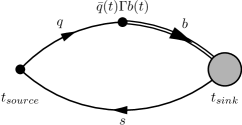
Figure 2: Three point correlator function used to obtain the $B_{s}\to\phi$ and $B_{s}\to D_{s}$ form factors. Double lines correspond to $b$-quark propagators, light, strange and charm propagators are denoted with single lines.

The conventional parametrization of $b\to s$ matrix elements is given by a set of seven form factors $f_{V}$, $f_{A_{0}}$, $f_{A_{1}}$, $f_{A_{2}}$, $f_{T_{1}}$, $f_{T_{2}}$ and $f_{T_{3}}$ [34]:

$$\langle\phi(k,\lambda)|\bar{s}\gamma^{\mu}b|{B_{s}}(p)\rangle ={f_{\phi}(q^{2})}\frac{2i\epsilon^{\mu\nu\rho\sigma}\varepsilon_{\nu}^{*}k_{\rho}p_{\sigma}}{M_{B_{s}}+M_{\phi}}\;,$$ (5)

$$\langle\phi(k,\lambda)|\bar{s}\gamma^{\mu}\gamma_{5}b|{B_{s}}(p)\rangle ={f_{A_{0}}(q^{2})}\frac{2M_{\phi}\varepsilon^{*}\cdot q}{q^{2}}q^{\mu}$$

$$\quad+{f_{A_{1}}(q^{2})}(M_{B_{s}}+M_{\phi})\left[\varepsilon^{*\mu}-\frac{\varepsilon^{*}\cdot q}{q^{2}}q^{\mu}\right]$$

$$\quad-{f_{A_{2}}(q^{2})}\frac{\varepsilon^{*}\cdot q}{M_{B_{s}}+M_{\phi}}\left[k^{\mu}+p^{\mu}-\frac{M_{B_{s}}^{2}-M_{\phi}^{2}}{q^{2}}q^{\mu}\right]\;,$$ (6)

$$q_{\nu}\langle\phi(k,\lambda)|\bar{s}\sigma^{\nu\mu}b|{B_{s}}(p)\rangle =2{f_{T_{1}}(q^{2})}\epsilon^{\mu\rho\tau\sigma}\varepsilon_{\rho}^{*}k_{\tau}p_{\sigma}\;,$$ (7)

$$q_{\nu}\langle\phi(k,\lambda)|\bar{s}\sigma^{\nu\mu}\gamma^{5}b|{B_{s}}(p)\rangle =i{f_{T_{2}}(q^{2})}\left[\varepsilon^{*\mu}(M_{B_{s}}^{2}-M_{\phi}^{2})-(\varepsilon^{*}\cdot q)(p+k)^{\mu}\right]$$

$$\quad+i{f_{T_{3}}(q^{2})}(\varepsilon^{*}\cdot q)\left[q^{\mu}-\frac{q^{2}}{M_{B_{s}}^{2}-M_{\phi}^{2}}(p+k)^{\mu}\right]\;.$$ (8)

In Equations (5)-(8), the 4-momenta of the $B_{s}$ and $\phi$ mesons are given by $p$ and $k$, respectively, $M_{B_{s}}$ and $M_{\phi}$ denote the corresponding meson masses, and $q=p-k$ is the momentum transfer. The calculation is carried out in the $B_{s}$-meson rest frame i.e. $q=(M_{B_{s}}-E_{\phi}(|\vec{k}|),-\vec{k})$ . The helicity and polarization vector of the $\phi$ meson are denoted by $\lambda$ and $\varepsilon$, respectively. The matrix elements in (5)-(8) are obtained from the ratio

$$R_{B_{s}\to\phi}^{\alpha\Gamma}(t,t_{\text{sink}},{k}) =\frac{C_{B_{s}\to\phi}^{\alpha\Gamma}(t,t_{\text{sink}},{k})}{\sqrt{\frac{1}{3}\sum_{i}C^{ii}_{\phi}(t,{k})C_{B_{s}}(t_{\text{sink}}-t)}}\sqrt{\frac{4E_{\phi}M_{B_{s}}\sum_{\lambda}\varepsilon^{j}(k,\lambda)\varepsilon^{j*}(k,\lambda)}{e^{-E_{\phi}t}e^{-M_{B_{s}}(t_{\text{sink}}-t)}}}$$ (9)

$$\xrightarrow{t\to\infty,\;t_{\text{sink}}-t\to\infty}\sum_{\lambda}\varepsilon^{\alpha}(k,\lambda)\langle\phi(k,\lambda)|\bar{q}\Gamma b|B_{s}(p)\rangle\;,$$ (10)

with the 3-point functions

$$C^{\alpha\Gamma}_{B_{s}\to\phi}(t,t_{\text{sink}},\vec{k})=\sum_{\vec{x},\vec{y}}e^{i\vec{k}\cdot\vec{y}}\langle\phi(0,\vec{0};\lambda)\bar{q}(t,\vec{y})\Gamma b(t,\vec{y})B_{s}(t_{\text{sink}},\vec{x})\rangle.$$ (11)

We sketch the 3-point functions in Fig. 2 and calculate them by contracting a sequential $b$-quark with a strange quark propagator via a vector or tensor current $\bar{q}\Gamma b$ with $\Gamma=\{\gamma^{\mu},\gamma^{5}\gamma^{\mu},\sigma^{\mu\nu},\gamma^{5}\sigma^{\mu\nu}\}$. The result is projected onto states of discrete momenta $\vec{k}$. The amplitudes obtained from Eq. (10) allow the straightforward extraction of the form factors $f_{A_{0}},f_{A_{1}},f_{T_{1}}$ and $f_{T_{2}}$. We extract the form factors $f_{A_{12}}$ and $f_{T_{23}}$ following the Cambridge group procedure Ref. [39]

$$f_{A_{12}}(q^{2}) =\frac{\sqrt{q^{2}}|\vec{k}|}{8M_{B_{s}}E_{\phi}k_{m}}\epsilon^{*}_{0,\mu}R_{B_{s}\to\phi}^{m\gamma^{\mu}\gamma^{5}},$$ (12)

$$f_{T_{23}}(q^{2}) =i\frac{|\vec{k}|(M_{B_{s}}+M_{\phi})}{4E_{\phi}k_{m}\sqrt{q^{2}}M_{B_{s}}}\epsilon^{*}_{0,\mu}q_{\nu}R_{B_{s}\to\phi}^{m\sigma^{\mu\nu}\gamma^{5}},$$ (13)

where

$$\epsilon^{*}_{0,\mu}=\frac{1}{\sqrt{q^{2}}}\left(|\vec{k}|,(E_{\phi}-M_{B_{s}})\frac{\vec{k}}{|\vec{k}|}\right).$$ (14)

For our basis of form factors $f_{V}$, $f_{A_{0}}$, $f_{A_{1}}$, $f_{A_{12}}$, $f_{T_{1}}$, $f_{T_{2}}$ and $f_{T_{23}}$, we perform correlated, constant in time fits up to discretized momenta of $\vec{k}=2\pi(1,1,1)/L$. Within our fitting ranges contamination from excited states is not visible and we use the same fitting ranges for all momenta and ensembles at the same lattice spacing. Fitting ranges for the $32^{3}$ ensembles are obtained by scaling our choices on $24^{3}$ using the ratio of the lattice spacings. The resulting form factors are then renormalized following the mostly non-perturbative method introduced in [44, 45]

$$\langle\phi(k,\lambda)|{\cal J}|B_{s}(p)\rangle=\rho^{bs}_{J}\sqrt{Z_{J}^{ss}Z_{J}^{bb}}\langle\phi(k)|J|B_{s}(p)\rangle,$$ (15)

where $\cal{J}$ and $J$ are the continuum and lattice current operators, respectively. We determine the flavor-conserving renormalizaton factors nonperturbatively in the chiral limit ($Z^{ss}_{J}=Z^{ll}_{J}$) and compute $\rho^{bs}_{J}$ at one loop in mean-field improved lattice perturbation theory for $J=\{\gamma^{\mu},\gamma^{\mu}\gamma^{5}\}$. For tensorial currents we set the $\rho^{bs}_{J}$ factor to its tree-level value because to date no perturbative one-loop calculation has been pursued. Our preliminary results for the seven renormalized form factors are presented in Figs. 3 and 4. In Figure 3 we show plots of the form factors for our coarse ensemble with $am_{l}=0.005$ using fixed $t_{\text{sink}}-t_{\text{source}}=20$ and show the dependence on the time slices $t$ in between. The error bands show the values for specific momenta extracted from a correlated, constant in time fit. Figure 4 shows the form factors versus the squared energy of the hadronic final state ($\phi$) indicating the physical $\phi$ mass by the dashed line on the left.

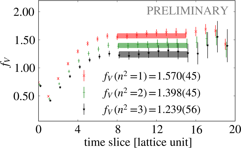
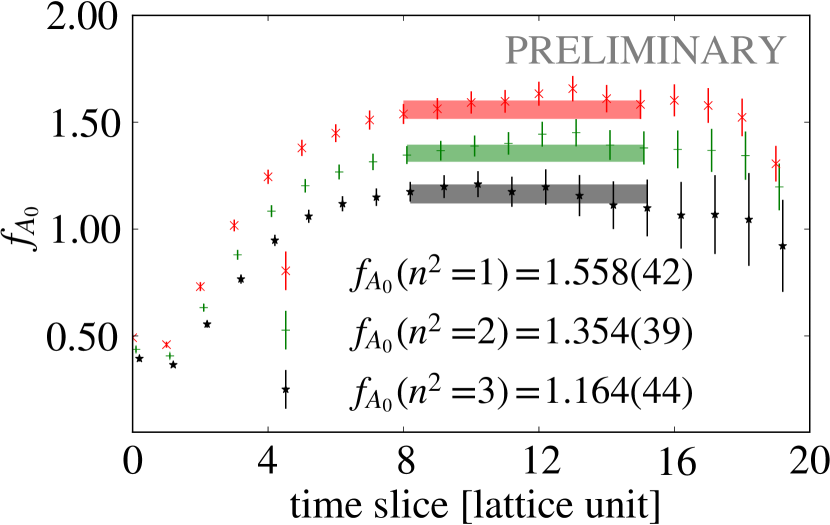
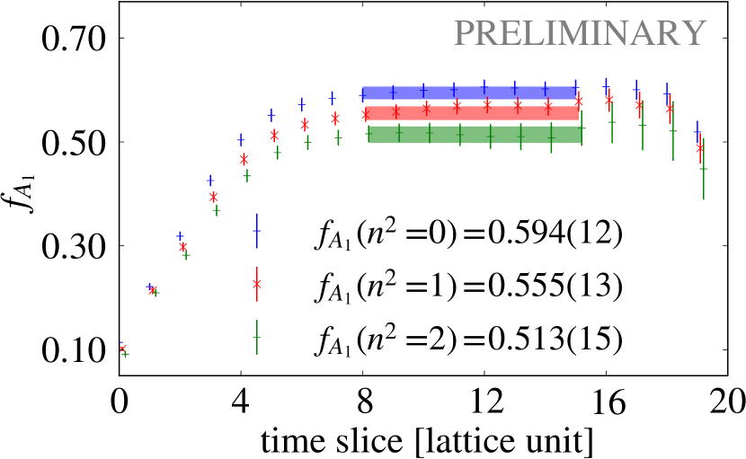
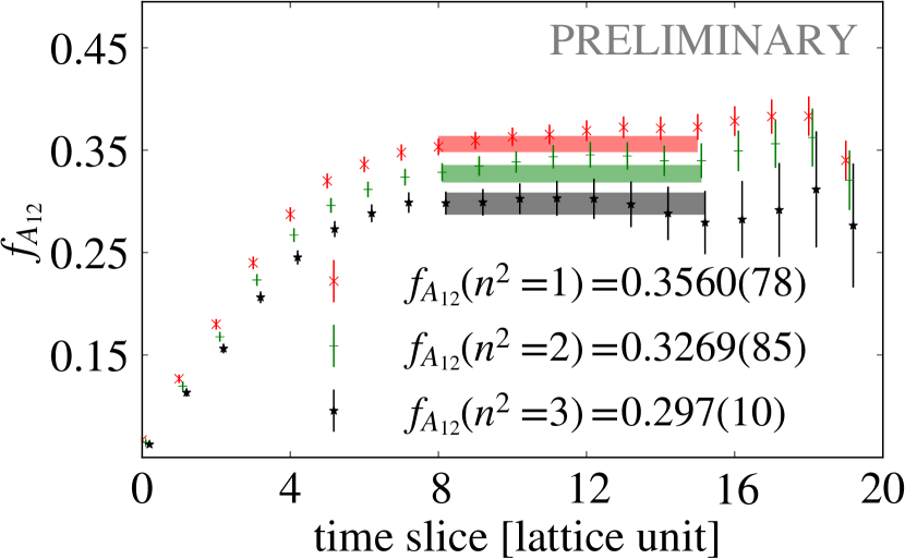
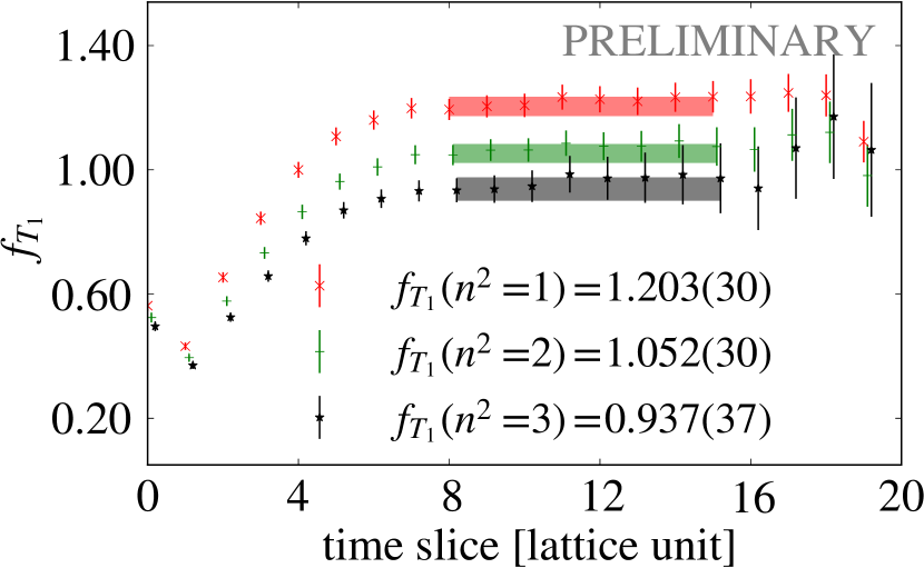
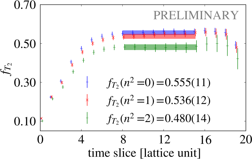
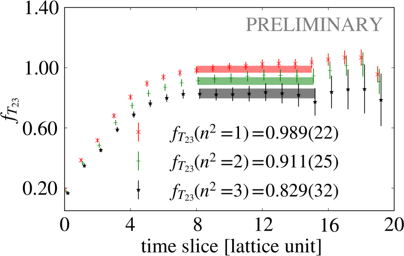
Figure 3: Effective mass style plots showing the determination of the seven form factors $f_{V}$, $f_{A_{0}}$,$f_{A_{1}}$, $f_{A_{12}}$, $f_{T_{1}}$, $f_{T_{2}}$ and $f_{T_{23}}$ for $B_{s}\to\phi\ell^{+}\ell^{-}$ for the coarse ensemble ($a^{-1}=1.785$ GeV) with $am_{l}=0.005$ and $t_{\text{sink}}-t_{\text{source}}=20$. We extract the values from correlated, constant in time fits to appropriate linear combinations of ratios of 3-point over 2-point functions. Fitting ranges are indicated by the length of the shaded error band.

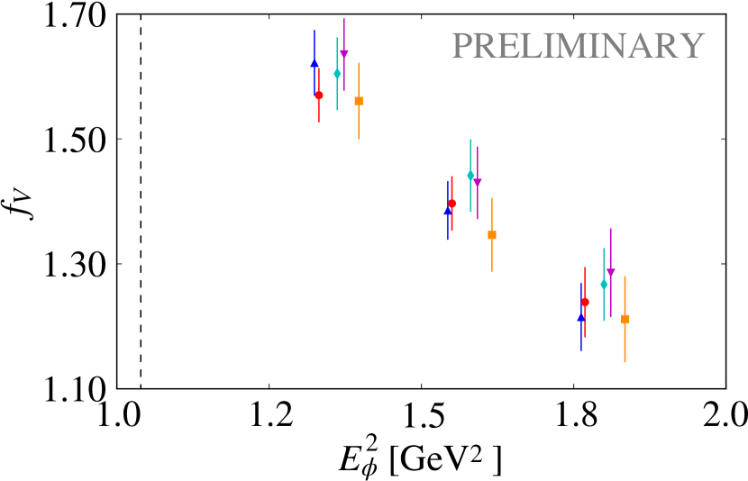
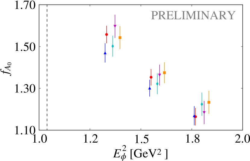
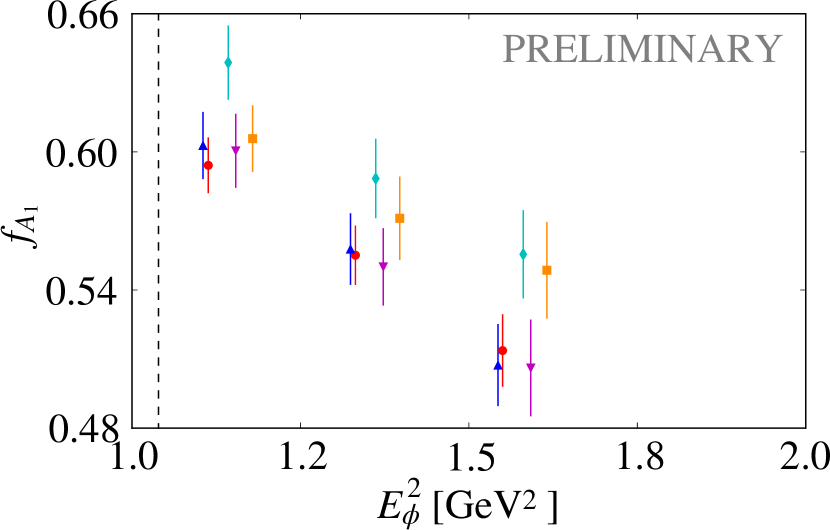
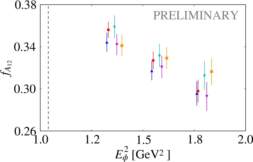
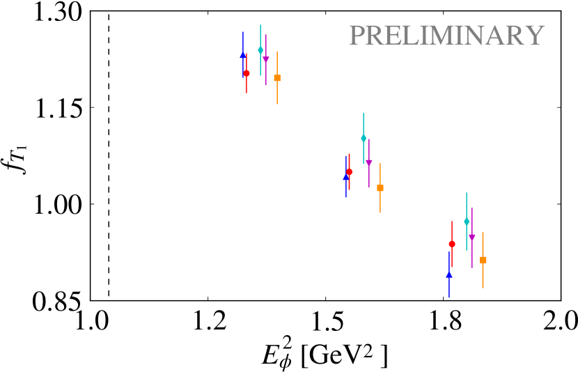
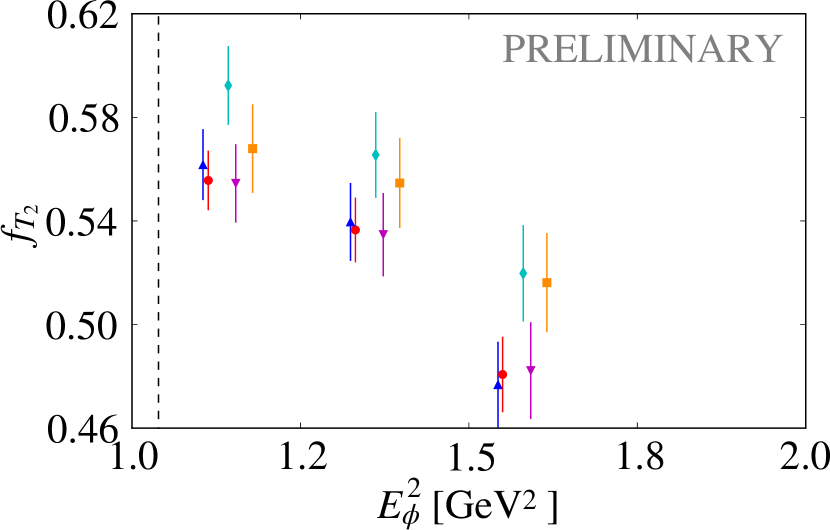
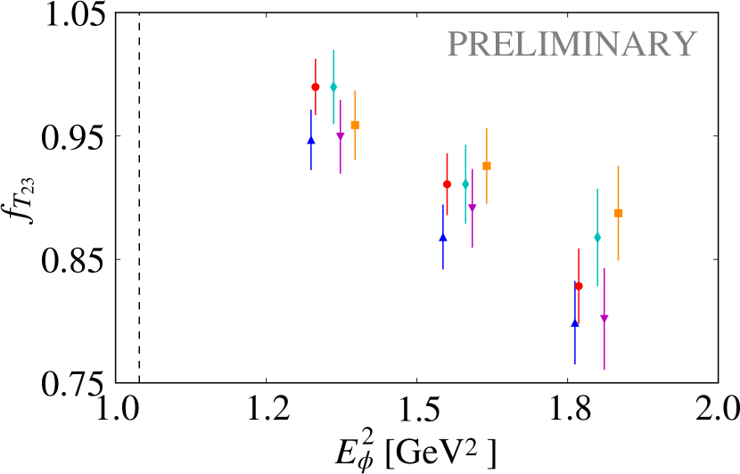
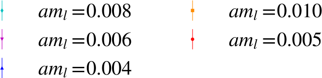
Figure 4: Renormalized results for the seven form factors $f_{V},f_{A_{0}},f_{A_{1}},f_{A_{12}},f_{T_{1}},f_{T_{2}}$ and $f_{T_{23}}$ for $B_{s}\to\phi\ell^{+}\ell^{-}$ versus the squared energy of the hadronic final state. Shown data are obtained on five different ensembles: sea-quark masses $am_{l}$ = 0.005, 0.010 correspond to the coarse lattice spacing $a^{-1}=1.785$ GeV and $am_{l}$ = 0.004, 0.006, 0.008 to the medium fine lattice spacing of $a^{-1}=2.383$ GeV. The dashed lines indicate the physical $\phi$ mass.

4 Semi-leptonic decays with $b\to c$ transitions

In order to determine semi-leptonic form factors for bottom quarks transitioning to charm quarks, we need a prescription for simulating charm quarks on the lattice. Since the mass of the charm quark ($m_{c}^{\overline{\text{MS}}}(\mu=m_{c})=1.27$ GeV [46]) is less than our smallest cutoff ($a^{-1}=1.730$ GeV), we may either use an effective action like RHQ or a fully relativistic formulation based on domain-wall fermions to simulate charm quarks. While the RHQ action is numerically cheaper, simulating charm with domain-wall fermions has the advantage that we match the action used for light and strange quarks. This avoids tuning the three parameters of the RHQ action and allows us to use a renormalization procedure similar to that in our $B\to\pi\ell\nu$ calculation. We therefore simulate charm based on the recent work featuring optimized Möbius domain-wall fermions [47, 48, 49, 15] i.e. we use domain-wall fermions with the Möbius kernel and choose the following parameters:

$$L_{s} =12 5^{th}$$ (extent of the dimension)

$$M_{5} =1.6$$ (domain-wall height)

$$b=1.5\quad \text{and}\quad c=0.5$$ (Möbius parameters) (16)

without link-smearing the gauge field [50, 49]. With this set-up, discretization errors have been shown to remain small for quantities like the charmonium mass $\eta_{c}$ or $D_{(s)}$ meson masses and decay constants if bare input quark masses below $am_{q}\lesssim 0.4$ are chosen [48]. Thus on our coarse ensembles ($a^{-1}\approx 1.78$ GeV), we cannot directly simulate charm quarks but expect a linear extrapolation to be benign [49, 15]. We simulate 2-3 charm-like quark masses and will subsequently extra-/interpolate to the physical charm quark mass. The bare charm quark masses used in our simulations as well as the $\eta_{c}$ masses relevant for a future extra-/interpolation are listed in Tab. 2.

$L^{3}\times T$	$a^{-1}$[GeV]	$am_{l}$	$am_{h}$	$am_{c}^{\text{sim}}$	$\eta_{c}^{\text{sim}}$[GeV]
$24^{3}\times 64$	1.785(5)	0.005	0.040	0.30, 0.35, 0.40	2.2246(62), 2.4492(68), 2.6604(74)
$24^{3}\times 64$	1.785(5)	0.010	0.040	0.30, 0.35, 0.40	2.2257(62), 2.4501(68), 2.6612(74)
$32^{3}\times 64$	2.383(9)	0.004	0.030	0.28, 0.34	2.6985(97), 3.059(11)
$32^{3}\times 64$	2.383(9)	0.006	0.030	0.28, 0.34	2.6990(97), 3.059(11)
$32^{3}\times 64$	2.383(9)	0.008	0.030	0.28, 0.34	determination in progress

Table 2: Simulated charm-like bare input quark masses $am_{c}^{\text{sim}}$ and the corresponding values of the $\eta_{c}^{\text{sim}}$ meson masses in GeV (connected $c\bar{c}$ contributions only) for our $24^{3}$ and $32^{3}$ ensembles. The physical $\eta_{c}$ mass is $\eta_{c}^{\text{phys}}=2.9834(5)$ GeV [46].

Before starting the form factor calculation, we first explored the signal of charm-light and charm-strange 2-point functions. We repeated a study investigating Gaussian smeared sources for the charm quarks with different widths $\sigma$ similar to the one presented in [24]. In Figure 5 we show the outcome of this study by plotting effective masses for $D_{s}$-like mesons on the left and $D_{s}^{*}$-like mesons on the right obtained on the coarse $24^{3}$ ensemble with $am_{l}=0.005$. As can be seen in the plots, the green data corresponding to a width $\sigma=7.86$ and $N_{\text{smear}}=100$ Jacobi iterations result in the earliest onset of the plateau which also extends over many time slices. Incidentally this is the same outcome as we found in our study for bottom quarks. Hence we will use the same choice for the Gaussian smearing in the following. Likewise we verified that the same separation of source and sink is suitable and results in a good plateau when analyzing the 3-point functions.

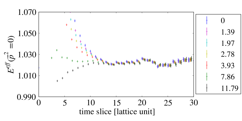
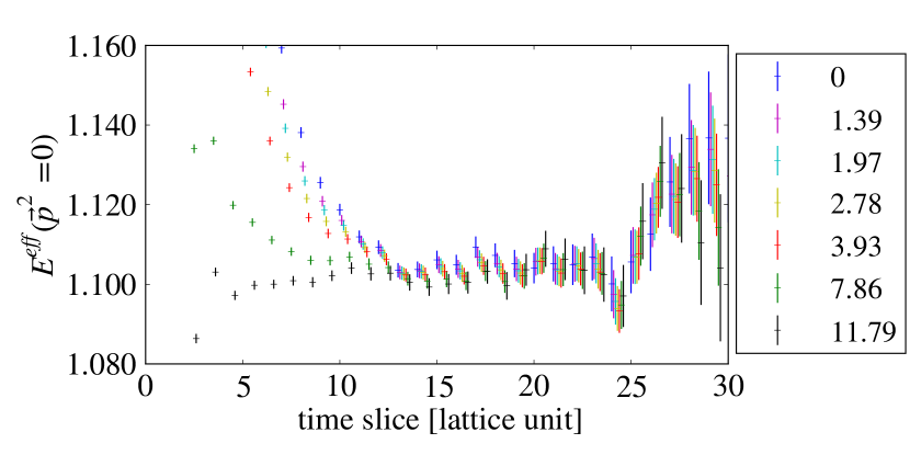
Figure 5: Exploring different widths $\sigma$ of the Gaussian source used to generate charm quarks by comparing effective masses for the $D_{s}$-like meson on the left and the $D_{s}^{*}$-like meson on the right. Strange quarks are generated with a point source and both propagators are contracted with a point sink. The data are obtained on the coarse $24^{3}$ ensemble with $am_{l}=0.005$ using $am_{s}^{\text{sim}}=0.03224$ and $am_{c}^{\text{sim}}=0.400$.

In the following we restrict ourselves to $D_{(s)}$ pseudoscalar final states and introduce the standard form factors $f_{+}$ and $f_{0}$ for semileptonic pseudoscalar-to-pseudoscalar decays

$$\langle D_{(s)}(k)|\bar{c}\gamma_{\mu}b|B_{(s)}(p)\rangle=f_{+}(q^{2})\left(p_{\mu}+k_{\mu}-\frac{M^{2}_{B_{(s)}}-M^{2}_{D_{(s)}}}{q^{2}}\right)+f_{0}(q^{2})\frac{M^{2}_{B_{(s)}}-M^{2}_{D_{(s)}}}{q^{2}}q_{\mu},$$ (17)

where $p$ is the 4-momentum of the $B_{(s)}$ meson, $k$ the 4-momentum of the $D_{(s)}$ meson, and $q\equiv(p-k)$, the momentum transferred to the outgoing charged-lepton-neutrino pair. As before we carry out our calculation in the $B_{(s)}$-meson rest frame i.e. $q=\left(M_{B_{(s)}}-E_{D_{(s)}}(|\vec{k}|),\;\;-\vec{k}\right)$.

The form factors introduced in Eq. (17) are defined in the continuum and related by the bottom-charm renormalization factor $Z_{V_{\mu}}^{bc}$ to the matrix elements we determine on the lattice

$$\langle D_{(s)}(k)|{\cal V}_{\mu}|B_{(s)}(p)\rangle=Z_{V_{\mu}}^{bc}\langle D_{(s)}(k)|V_{\mu}|B_{(s)}(p)\rangle.$$ (18)

The continuum vector current operator is denoted by ${\cal V}_{\mu}=\bar{c}\gamma_{\mu}b$ and $V_{\mu}$ is the corresponding lattice current operator. Again we obtain the renormalization factor by rewriting it according to the mostly non-perturbative method [44, 45]

$$Z_{V_{\mu}}^{bc}=\rho^{bc}_{V_{\mu}}\sqrt{Z_{V}^{cc}Z_{V}^{bb}},$$ (19)

where the flavor conserving factors are determined non-perturbatively and only the remaining $\rho$-factor is determined using lattice perturbation theory.

Following the prescription given in Refs. [51, 52], $Z_{V}^{cc}$ is obtained in the chiral limit using the domain-wall height $M_{5}$ chosen to simulate charm quarks. In Figure 6 we show our preliminary results for $B_{s}\to D_{s}\ell\nu$ semi-leptonic decays in terms of the form factors $f_{\parallel}$ and $f_{\perp}$ obtained on the $24^{3}$ ensembles with $a^{-1}=1.785$ GeV. $f_{\parallel}$ and $f_{\perp}$ are linearly related to the physical form factors $f_{+}$ and $f_{0}$. These data have yet to be renormalized and are based on the tree-level operator only. We show discretized momenta up to $\vec{k}=2\pi\vec{n}/L$ with $\vec{n}$ up to $(2,0,0)$ and average spatial directions with the same $|n|$.

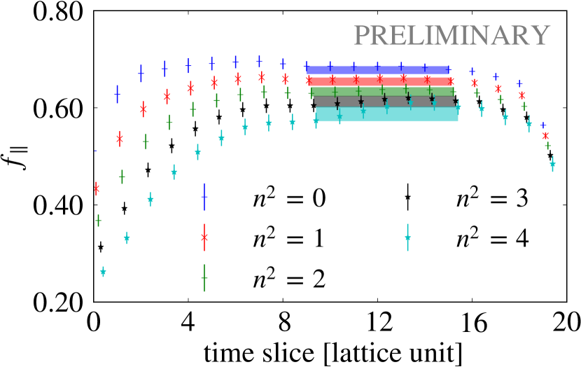
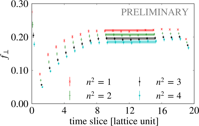
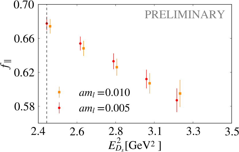
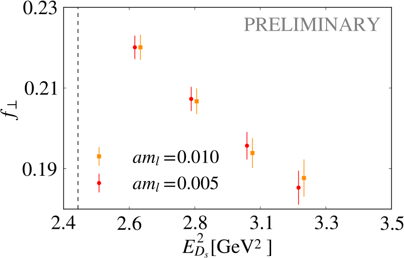
Figure 6: Preliminary results for our determination of semi-leptonic form factors for $B_{s}\to D_{s}\ell\nu$. On the left we show $f_{\parallel}$, on the right $f_{\perp}$. The upper plots show fits to the linear combination of ratios of 3-point over 2-point functions determining the form factor for the coarse ensemble ($a^{-1}=1.785$ GeV) with $am_{l}=0.005$ using $am_{c}^{\text{sim}}=0.300$. In the lower plots we show our results for both coarse ensembles as a function of the squared energy of the $D_{s}$-like meson. The mass of the $D_{s}$-like meson is indicated by the black dashed line.

5 Outlook and conclusions

We have reported on the status of our program to compute semi-leptonic $B$ decays. The full program considers pseudoscalar $B$ or $B_{s}$ mesons in the initial state and a single pseudoscalar or vector meson in the final state. Vector final states are treated as stable within the narrow width approximation. Here we show updates for our calculation of GIM suppressed $B_{s}\to\phi\ell^{+}\ell^{-}$ decays and presented first results for computing $b\to c$ transitions as they occur e.g. in $B_{s}\to D_{s}\ell\nu$.

Most of our numerical simulations have been completed on the $24^{3}$ and $32^{3}$ ensembles, but we are still accumulating data on the more costly $48^{3}$ ensembles. In parallel we are carrying out the perturbative calculations required for renormalizing and $O(a)$-improving the weak matrix elements calculated on the lattice and start to build-up our data analysis. Once we have $O(a)$-improved and renormalized data we will start to carry out combined chiral- and continuum extrapolations and for $B_{(s)}\to D_{(s)}^{(*)}\ell\nu$ decays will explore extra-/interpolating to the physical charm quark mass.

Acknowledgments

The authors thank our collaborators in the RBC and UKQCD Collaborations for helpful discussions and suggestions. Computations for this work were performed on resources provided by the USQCD Collaboration, funded by the Office of Science of the U.S. Department of Energy, as well as on computers at Columbia University and Brookhaven National Laboratory. This work used the ARCHER UK National Supercomputing Service (http://www.archer.ac.uk). Gauge field configurations on which our calculations are based were also generated using the DiRAC Blue Gene Q system at the University of Edinburgh, part of the DiRAC Facility; funded by BIS National E-infrastructure grant ST/K000411/1 and STFC grants ST/H008845/1, ST/K005804/1 and ST/K005790/1. This project has received funding from the European Union’s Horizon 2020 research and innovation programme under the Marie Skłodowska-Curie grant agreement No 659322, the European Research Council under the European Unions Seventh Framework Programme (FP7/ 2007-2013) / ERC Grant agreement 279757, STFC grant ST/L000296/1 and ST/L000458/1 as well as the EPSRC Doctoral Training Centre grant (EP/G03690X/1). No new experimental data was generated for this research.

References

- Glashow et al. [1970] S. L. Glashow, J. Iliopoulos, and L. Maiani, Phys. Rev. D2, 1285 (1970)
- Aaij et al. [2016] R. Aaij et al. (LHCb), JHEP 02, 104 (2016), arXiv:1512.04442 [hep-ex]
- Aaij et al. [2015] R. Aaij et al. (LHCb), JHEP 09, 179 (2015), arXiv:1506.08777 [hep-ex]
- Aaij et al. [2014] R. Aaij et al. (LHCb), Phys. Rev. Lett. 113, 151601 (2014), arXiv:1406.6482 [hep-ex]
- Fajfer et al. [2012] S. Fajfer, J. F. Kamenik, and I. Nisandzic, Phys. Rev. D85, 094025 (2012), arXiv:1203.2654 [hep-ph]
- Bailey et al. [2012] J. A. Bailey et al., Phys. Rev. Lett. 109, 071802 (2012), arXiv:1206.4992 [hep-ph]
- Lees et al. [2012] J. Lees et al. (BaBar), Phys.Rev.Lett. 109, 101802 (2012), arXiv:1205.5442 [hep-ex]
- Nandi et al. [2016] S. Nandi, S. K. Patra, and A. Soni, (2016), arXiv:1605.07191 [hep-ph]
- Flynn et al. [2015] J. M. Flynn, T. Izubuchi, T. Kawanai, C. Lehner, A. Soni, R. S. Van de Water, and O. Witzel, Phys. Rev. D91, 074510 (2015), arXiv:1501.05373 [hep-lat]
- Flynn et al. [2016] J. Flynn, A. Jüttner, T. Kawanai, E. Lizarazo, and O. Witzel, PoS LATTICE2015, 345 (2016), arXiv:1511.06622 [hep-lat]
- Bigi and Gambino [2016] D. Bigi and P. Gambino, Phys. Rev. D94, 094008 (2016), arXiv:1606.08030 [hep-ph]
- Allton et al. [2008] C. Allton et al. (RBC-UKQCD), Phys. Rev. D78, 114509 (2008), arXiv:0804.0473 [hep-lat]
- Aoki et al. [2011] Y. Aoki et al. (RBC-UKQCD), Phys.Rev. D83, 074508 (2011), arXiv:1011.0892 [hep-lat]
- Blum et al. [2016] T. Blum et al. (RBC, UKQCD), Phys. Rev. D93, 074505 (2016), arXiv:1411.7017 [hep-lat]
- Boyle et al. [2016a] P. A. Boyle et al., “in preparation,” (2016a)
- Shamir [1993] Y. Shamir, Nucl. Phys. B406, 90 (1993), arXiv:hep-lat/9303005
- Furman and Shamir [1995] V. Furman and Y. Shamir, Nucl. Phys. B439, 54 (1995), arXiv:hep-lat/9405004
- Brower et al. [2012] R. C. Brower, H. Neff, and K. Orginos, (2012), arXiv:1206.5214 [hep-lat]
- Iwasaki [1983] Y. Iwasaki, UTHEP-118 (1983)
- El-Khadra et al. [1997] A. X. El-Khadra, A. S. Kronfeld, and P. B. Mackenzie, Phys. Rev. D55, 3933 (1997), arXiv:hep-lat/9604004
- Lin and Christ [2007] H.-W. Lin and N. Christ, Phys.Rev. D76, 074506 (2007), arXiv:hep-lat/0608005
- Christ et al. [2007] N. H. Christ, M. Li, and H.-W. Lin, Phys.Rev. D76, 074505 (2007), arXiv:hep-lat/0608006
- Sheikholeslami and Wohlert [1985] B. Sheikholeslami and R. Wohlert, Nucl.Phys. B259, 572 (1985)
- Aoki et al. [2012] Y. Aoki, N. H. Christ, J. M. Flynn, T. Izubuchi, C. Lehner, M. Li, H. Peng, A. Soni, R. S. Van de Water, and O. Witzel (RBC-UKQCD), Phys. Rev. D86, 116003 (2012), arXiv:1206.2554 [hep-lat]
- Alford et al. [1996] M. G. Alford, T. Klassen, and P. Lepage, Nucl.Phys.Proc.Suppl. 47, 370 (1996), arXiv:hep-lat/9509087 [hep-lat]
- Grinstein et al. [1988] B. Grinstein, R. P. Springer, and M. B. Wise, Phys. Lett. B202, 138 (1988)
- Grinstein et al. [1990] B. Grinstein, R. P. Springer, and M. B. Wise, Nucl. Phys. B339, 269 (1990)
- Buras et al. [1994] A. J. Buras, M. Misiak, M. Munz, and S. Pokorski, Nucl. Phys. B424, 374 (1994), arXiv:hep-ph/9311345 [hep-ph]
- Ciuchini et al. [1993] M. Ciuchini, E. Franco, G. Martinelli, L. Reina, and L. Silvestrini, Phys. Lett. B316, 127 (1993), arXiv:hep-ph/9307364 [hep-ph]
- Ciuchini et al. [1994a] M. Ciuchini, E. Franco, L. Reina, and L. Silvestrini, Nucl. Phys. B421, 41 (1994a), arXiv:hep-ph/9311357 [hep-ph]
- Ciuchini et al. [1994b] M. Ciuchini, E. Franco, G. Martinelli, L. Reina, and L. Silvestrini, Phys. Lett. B334, 137 (1994b), arXiv:hep-ph/9406239 [hep-ph]
- Buras et al. [2002] A. J. Buras, A. Czarnecki, M. Misiak, and J. Urban, Nucl. Phys. B631, 219 (2002), arXiv:hep-ph/0203135 [hep-ph]
- Gambino et al. [2003] P. Gambino, M. Gorbahn, and U. Haisch, Nucl. Phys. B673, 238 (2003), arXiv:hep-ph/0306079 [hep-ph]
- Altmannshofer et al. [2009] W. Altmannshofer, P. Ball, A. Bharucha, A. J. Buras, D. M. Straub, and M. Wick, JHEP 01, 019 (2009), arXiv:0811.1214 [hep-ph]
- Grinstein and Pirjol [2004] B. Grinstein and D. Pirjol, Phys. Rev. D70, 114005 (2004), arXiv:hep-ph/0404250 [hep-ph]
- Beylich et al. [2011] M. Beylich, G. Buchalla, and T. Feldmann, Eur. Phys. J. C71, 1635 (2011), arXiv:1101.5118 [hep-ph]
- Lyon and Zwicky [2014] J. Lyon and R. Zwicky, (2014), arXiv:1406.0566 [hep-ph]
- Horgan et al. [2014a] R. R. Horgan, Z. Liu, S. Meinel, and M. Wingate, Phys. Rev. Lett. 112, 212003 (2014a), arXiv:1310.3887 [hep-ph]
- Horgan et al. [2014b] R. R. Horgan, Z. Liu, S. Meinel, and M. Wingate, Phys. Rev. D89, 094501 (2014b), arXiv:1310.3722 [hep-lat]
- Horgan et al. [2015] R. R. Horgan, Z. Liu, S. Meinel, and M. Wingate, PoS LATTICE2014, 372 (2015), arXiv:1501.00367 [hep-lat]
- Bouchard et al. [2013] C. Bouchard, G. P. Lepage, C. Monahan, H. Na, and J. Shigemitsu (HPQCD), Phys. Rev. Lett. 111, 162002 (2013), [Erratum: Phys. Rev. Lett.112,no.14,149902(2014)], arXiv:1306.0434 [hep-ph]
- Bailey et al. [2016] J. A. Bailey et al., Phys. Rev. D93, 025026 (2016), arXiv:1509.06235 [hep-lat]
- Du et al. [2016] D. Du, A. X. El-Khadra, S. Gottlieb, A. S. Kronfeld, J. Laiho, E. Lunghi, R. S. Van de Water, and R. Zhou, Phys. Rev. D93, 034005 (2016), arXiv:1510.02349 [hep-ph]
- Hashimoto et al. [1999] S. Hashimoto, A. X. El-Khadra, A. S. Kronfeld, P. B. Mackenzie, S. M. Ryan, and J. N. Simone, Phys. Rev. D61, 014502 (1999), arXiv:hep-ph/9906376 [hep-ph]
- El-Khadra et al. [2001] A. X. El-Khadra et al., Phys.Rev. D64, 014502 (2001), arXiv:hep-ph/0101023
- Patrignani et al. [2016] C. Patrignani et al. (Particle Data Group), Chin. Phys. C40, 100001 (2016)
- Boyle et al. [2016b] P. Boyle, L. Del Debbio, A. Khamseh, A. Jüttner, F. Sanfilippo, and J. T. Tsang, PoS LATTICE2015, 336 (2016b), arXiv:1511.09328 [hep-lat]
- Boyle et al. [2016c] P. Boyle, A. Jüttner, M. K. Marinkovic, F. Sanfilippo, M. Spraggs, and J. T. Tsang, JHEP 04, 037 (2016c), arXiv:1602.04118 [hep-lat]
- Boyle et al. [2016d] P. Boyle, L. Del Debbio, A. Jüttner, A. Khamseh, F. Sanfilippo, J. T. Tsang, and O. Witzel, (2016d), arXiv:1611.06804 [hep-lat]
- Cho et al. [2015] Y.-G. Cho, S. Hashimoto, A. Jüttner, T. Kaneko, M. Marinkovic, J.-I. Noaki, and J. T. Tsang, JHEP 05, 072 (2015), arXiv:1504.01630 [hep-lat]
- Boyle et al. [2016e] P. Boyle, L. Del Debbio, and A. Khamseh, (2016e), arXiv:1608.07982 [hep-lat]
- Boyle et al. [2016f] P. Boyle, L. Del Debbio, and A. Khamseh, (2016f), arXiv:1611.06908 [hep-lat]