Compact star in pseudo-spheroidal spacetime

Abstract

We investigate perfect fluid stars in $(2+1)$ dimension in pseudo-spheroidal spacetime with the help of Vaidya-Tikekar metric where the physical $3$-space ($t=$ constant) is described by pseudo-spheroidal geometry. Here the spheroidicity parameter $a$, plays an important role for determining the properties of a compact star. In the present work a class of interior solutions corresponding to the Ba$\tilde{n}$ados-Teitelboim-Zanelli $(BTZ)$ (Bañados et al., Phys. Rev. Lett. 69:1849, 1992) exterior metric has been provided which describes a static circularly symmetric star with negative cosmological constant in equilibrium. It is shown that asymptotically anti-de Sitter $(2+1)$ dimensional spacetime described by BTZ admits a compact star solution with reasonable physical features.

Keywords General relativity; Pseudo-spheroidal spacetime; Compact star

1 Introduction

After the discovery of the particle named as Neutron by Chadwick, later on existence of the neutron star was predicted. A neutron star is the later stage of a gravitationally collapsed star. It becomes stabilized by the degenerate neutron pressure, after exhausting all its thermonuclear fuel. With the discovery of pulsars (Hewish et al., 1968) this concept got concrete experimental support. However the estimated mass and radius of different compact object such as X-ray pulsar $Her~{}X-1$, X-ray burster $4U~{}1820-30$, millisecond pulsar $SAX~{}J~{}1808.4-3658$ and X-ray sources $RX~{}J~{}185635-3754$ could not be described by the standard neutron star model. It is found by Ruderman (1972) that the matter densities of compact stars are to be of the order of $10^{15}$ gm/cc or higher, exceeding the nuclear matter density and at this high density range nuclear interactions must be treated relativistically. As a result of the anisotropy, pressure inside the fluid sphere can be decomposed into two parts namely radial pressure $p_{r}$ and the transverse pressure $p_{t}$, where $p_{t}$ is in the perpendicular direction to $p_{r}$. Anisotropy may occurs in various reasons e.g. the existence of solid core, in presence of type P superfluid, phase transition, rotation, magnetic field, mixture of two fluid, existence of external field etc (Thirukkanesh and Ragel, 2014). On the basis of compactification factor (ratio of mass and radius), the compact objects are classified into a normal star ($10^{-5}$), white dwarf ($10^{-3}$), neutron star ($0.1$ to $0.2$), strange star ($0.2$ to $<0.5$), black hole ($0.5$) etc. The physics and equation of state (EOS) of compact objects near the core region are still not known clearly.

To analyze a compact object Vaidya and Tikekar (1982) and Tikekar (1990) prescribed a simple form for the space like hyper surface ($t$= constant) containing two parameters, namely spheroidicity parameter $(a)$ and curvature parameter ($R$). The Vaidya-Tikekar approach reduces the complexity of field equations which produces solution of relativistic stars with ultra high densities and is also useful to obtain stellar solution for a compact star with Einstein-Maxwell field equations (Rhodes and Ruffini, 1974). The physics of the Vaidya-Tikekar metric is discussed in the Refs. (Vaidya and Tikekar, 1982; Knutsen, 1988; Tikekar, 1990). With different choice of spheroidal parameter Maharaja and Leach (1996) obtained a new classes of solutions for superdense stars. Thomas and Tikekar (1998) and Tikekar and Thomas (1999) obtained a class of relativistic solutions analyzing compact stars with $3$-pseudo-spheroidal geometry for the $3$-space of the interior spacetime. Considering the anisotropic distribution of fluid including pseudo-spheroidal geometry to construct compact star models one may look at the Refs. (Patel and Mehta, 1995; Jotania and Tikekar, 2005). In connection to compact star in one of our earlier works (Shee et al., 2016) we proposed a model for relativistic dense star with anisotropy that admits non-static conformal symmetry.

Actively researching in the field of lower dimensional gravity one can understand substantially some of the crucial points of astrophysics. Lower dimensional analysis of black holes has often been preferred to understand the various issues which are to be difficult to resolve in conventional dimensions.  Banados et al. (1992) (henceforth BTZ) obtained a beautiful solution which opened up the possibility of investigating many interesting features of black holes. They obtained a analytical solution representing the exterior gravitational field of a black hole in $(2+1)$ dimensions in the presence of negative cosmological constant. Mann and Ross (1993) analyzed collapsing dust cloud ($p=0$) in $(2+1)$ dimensions leading to a black hole. Later on Martins et al. (2010) obtained a self similar solution in $(2+1)$ dimensions by considering the collapse of a circularly symmetric anisotropic fluid. The interior solution for an incompressible fluid in $(2+1)$ dimensions and the bound on the maximum allowed mass of the resulting configuration was obtained by Cruz and Zanelli (1995). The study also claims that the collapsed stage would always be covered under its event horizon. A class of interior solutions corresponding to BTZ exterior was provided by Cruz et al. (2005) by assuming a particular density profile $\rho=\rho_{c}(1-\frac{r^{2}}{R^{2}})$, where $\rho_{c}$ is the central density, $\rho$ is the density which is a function of the radial parameter $r$ and $R$ is the boundary of the star. Assuming polytropic EOS, such as $p=K\rho^{1+\frac{1}{n}}$, Paulo (1999) proposed a interior solution corresponding to the BTZ exterior, where $n$ is the polytropic index and $K$ is the polytropic constant. A new class of interior solution corresponding to the BTZ exterior was provided by Sharma et al. (2011) by assuming a particular form of mass function $2m(r)=C-e^{-2\mu(r)}-\Lambda r^{2}$, where $\mu(r)$ is the metric function and $m(r)$ is the mass within the radial distance. The general BTZ metric is characterized by its mass, angular momentum and electric charge but is asymptotically anti-de Sitter rather than flat (Husain, 1995).

Being motivated by the above background works we have presented here a compact star model under ($2+1$) dimensional metric with several interesting physical properties. The plan of the investigation is as follows: In the Sec. 2 we have provided necessary spacetime background and hence the Einstein field equations in the presence of cosmological constant. We have found solutions for different physical parameters and matching condition in the Secs. 3 and 4 respectively. In Sec. 5 we have explored different physical features, viz. the density and mass, pressure and anisotropy, stability, energy conditions, compactness and redshift etc. with elaborate discussion. In the last Sec. 6 we have made some concluding remarks regarding different aspects of the present model.

2 The spacetime metric

2.1 Interior spacetime

We take the following ($2+1$) dimensional metric describing the interior of a static spherically symmetric distribution of matter as

$$ds^{2}=-e^{2\gamma(r)}dt^{2}+e^{2\mu(r)}dr^{2}+r^{2}d\theta^{2}.$$ (1)

The energy-momentum tensor of the matter distribution in the interior of the star is given by

$$T_{ij}=(\rho+p_{r})u_{i}u_{j}+p_{t}g_{ij}+(p_{r}-p_{t})\chi_{i}\chi_{j},$$ (2)

where $\rho$ represents the energy density, $p_{r}$ is the radial pressure, $p_{t}$ is the tangential pressure, $g_{ij}$ are the metric tensors, $\chi^{i}=e^{-\mu(r)}\delta^{i}_{r}$ is a unit three vector along the radial direction, and $u^{i}$ are the $3$-velocity of the fluid.

The Einstein field equations with a cosmological constant under the specification $G=c=1$ are given by

$$2\pi\rho+\Lambda = \frac{\mu^{\prime}e^{-2\mu}}{r},$$ (3)

$$2\pi p_{r}-\Lambda = \frac{\gamma^{\prime}e^{-2\mu}}{r},$$ (4)

$$2\pi p_{t}-\Lambda = e^{-2\mu}\left(\gamma^{\prime 2}+\gamma^{\prime\prime}-\gamma^{\prime}\mu^{\prime}\right),$$ (5)

where a ‘$\prime$’ denotes differentiation with respect to the radial parameter $r$. Combining Eqs. (3)-(5), we have

$$\left(\rho+p_{r}\right)\gamma^{\prime}+p_{r}^{\prime}+\frac{1}{r}\left(p_{r}-p_{t}\right)=0,$$ (6)

which is the conservation equation in $(2+1)$ dimensions.

2.2 Metric potential

Since we take $(2+1)$ dimensions in pseudo spheroidal spacetime, therefore, we use the ansatz (Mann and Ross, 1993)

$$e^{2\mu}=\frac{1+\frac{ar^{2}}{R^{2}}}{1+\frac{r^{2}}{R^{2}}},$$ (7)

where $a$ is the spheroidicity parameter and $R$ is a geometrical parameter related with the configuration of the star model.

Using Eq. (7) we get

$$2\mu=ln\frac{R^{2}+ar^{2}}{R^{2}+r^{2}}.$$ (8)

Therefore differentiating $\mu$ with respect to $r$ we get

$$\mu^{\prime}=\frac{R^{2}r(a-1)}{(R^{2}+ar^{2})(R^{2}+r^{2})}.$$ (9)

The above equations are used to calculate $\rho$ and $p_{t}$. However, here it is to note that the spheroidicity parameter $a$ and curvature parameter $R$ plays a very important role in our work. We shall take $a=6$ and $R=22.882$ km through out the work as taken by Chattopadhyay et al. (2012) for X ray pulsar $Her-X-1$. It can be observed that the variation of these parametric values within the range $5<a<10$ and $20<R<25$ shows very negligible effect. However, for the present prescription on the numerical values of $a$ and $R$, we would add that though BTZ black hole is not a three-dimensional section of a $4D$ black hole however it facilitates to understand several key features of the model presented here.

3 The anisotropic stellar model

It is known that $\Lambda>0$ implies the space is open. To explain the present accelerating state of the universe, it is believed that vacuum energy is responsible for this expansion. As a consequence, it provides the gravitational effect on the stellar structures and this cosmological constant $(\Lambda)$ plays the role of vacuum energy or dark energy. In this section we will study the following features of our model assuming the value of $\Lambda=0.00018\ km^{-2}$ (Kalam et al., 2012). We have assumed this value as required for the stability of the compact star and mathematical consistency.

The matter density $(\rho)$ can be found from Eq. (3) as

$$\rho=\frac{1}{2\pi}\frac{R^{2}(a-1)}{(R^{2}+ar^{2})^{2}}-\frac{\Lambda}{2\pi}.$$ (10)

The variation of $\rho$ i.e. matter density with distance from the center of the star is given by

$$\rho^{\prime}=\frac{d\rho}{dr}=-\frac{4arR^{2}(a-1)}{2\pi(R^{2}+ar^{2})^{3}}<0.$$ (11)

The above expression implies that at $r=0$ the matter density remains constant. The second order derivative of $\rho$ with respect to the distance from the center of the star is given by

$$\rho^{\prime\prime}=\frac{d^{2}\rho}{dr^{2}}=-\frac{4aR^{2}(a-1)(R^{2}-5ar^{2})}{2\pi(R^{2}+ar^{2})^{4}}<0.$$ (12)

The variation of $\rho$, $\rho{{}^{\prime}}$ and $\rho{{}^{\prime\prime}}$ with the radial distance $r$ are shown in the Fig. 1.

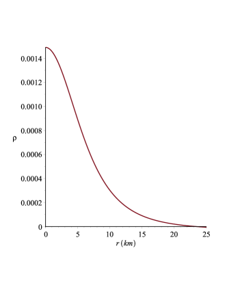
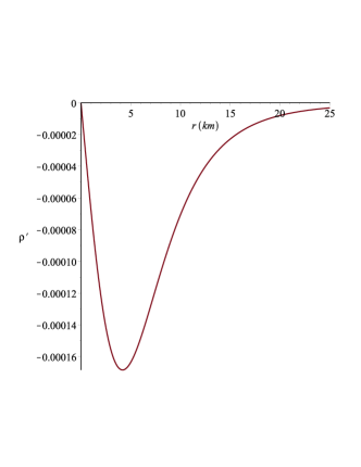
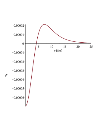
Fig. 1 : Variation of the $\rho$ (upper left), $\rho^{{}^{\prime}}$ (upper right) and $\rho^{{}^{\prime\prime}}$ (lower) with $r$

If we take $p_{r}=\omega\rho$ then we get the differential equation

$$\gamma^{\prime}=\frac{r}{(R^{2}+ar^{2})(R^{2}+r^{2})}\left[\omega(a-1)R^{2}-\right.$$

$$\left.\Lambda(\omega+1)(R^{2}+ar^{2})^{2}\right].$$ (13)

Integrating the above equation we can get $\gamma$ as

$$\gamma=\frac{\omega}{2}\ln\left(\frac{R^{2}+ar^{2}}{R^{2}+r^{2}}\right)-\frac{\Lambda}{2}(\omega+1)[ar^{2}-R^{2}\ln a]+D,$$ (14)

where $D$ is the integration constant which can be determined from boundary conditions.

Using Eqs. (7) and  (13) we can get the radial pressure $(p_{r})$ from Eq. (4) as

$$2\pi p_{r}=\frac{\omega(a-1)R^{2}}{(R^{2}+ar^{2})^{2}}-\Lambda\omega.$$ (15)

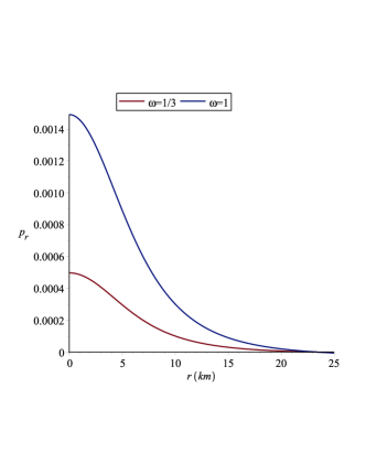
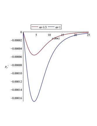
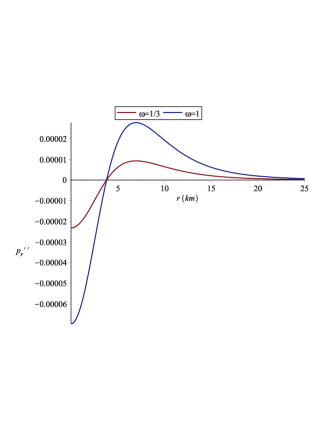
Fig. 2 : Variation of the $p_{r}$ (upper left), $p_{r}^{{}^{\prime}}$ (upper right) and $p_{r}^{{}^{\prime\prime}}$ (lower) with $r$

Now we shall calculate variation of the radial pressure $(p_{r})$ with the radius $(r)$ of the star as

$$2\pi\frac{dp_{r}}{dr}=-\frac{4\omega arR^{2}(a-1)}{(R^{2}+ar^{2})^{3}}<0.$$ (16)

From the above Eq. (15) we have the radial pressure $p_{r}$ is constant at $r=0$. The second order derivative of radial pressure with respect to radius of the star is given by

$$2\pi\frac{d^{2}p_{r}}{dr^{2}}=-\frac{4\omega aR^{2}(R^{2}-6ar^{2})(a-1)}{(R^{2}+ar^{2})^{4}}<0.$$ (17)

The variation of $p_{r}$, $p_{r}{{}^{\prime}}$ and $p_{r}{{}^{\prime\prime}}$ with the radial distance $r$ are shown in the Fig. 2. Since $\frac{d\rho}{dr},\frac{dp_{r}}{dr}<0$ we can conclude that both the matter density $(\rho)$ and radial pressure $(p_{r})$ are monotonic decreasing function of radius $r$. From Figs. 1 and 2 it can be observed that these parameters have maximum value at the center $(r=0)$ of the star and it decreases radially outward.

The variation of the radial pressure with respect to the matter density is given by

$$\frac{dp_{r}}{d\rho}=\omega=v_{rs}^{2},$$ (18)

and has been plotted in Fig. 6 which gives a constant value. This result physically implies that the radial pressure dose not changes with the matter density.

The EOS parameter corresponding to radial direction may be written as

$$\omega_{r}=\frac{p_{r}}{\rho}=\omega,$$ (19)

which is a constant quantity.

As $p_{r}=0$ and $\rho=0$ at $r=b$, the radius of compact star, we get the same result from Eqs. (10) and  (15) as

$$b=\sqrt{\frac{R}{a}\left(\sqrt{\frac{a-1}{\Lambda}}-R\right)}.$$ (20)

Putting the numerical values of the constants we get the radius of the star to be $23.417$ km which is exactly same as obtained from Figs. 1 and 2.

The tangential pressure is given by the following equation

$$2\pi p_{t}-\Lambda=\frac{1}{C^{3}(R^{2}+r^{2})}\left\{r^{2}\left[(AR^{2}-BC^{2})\right]\right.$$

$$\left.\times\left[R^{2}(A-a+1)-BC^{2}\right]\right.$$

$$\left.+AR^{2}[R^{4}-R^{2}r^{2}(a+1)-3ar^{4}]-\right.$$

$$\left.BC[R^{4}+R^{2}r^{2}(3a-1)+ar^{4}]\right\},$$ (21)

where $A=\omega(a-1)$, $B=\Lambda(\omega+1)$ and $C=R^{2}+ar^{2}$. The above equation shows that at $r=0$ the tangential pressure $p_{t}$ has a finite positive value. Due to complexity in the expression of $p_{t}{{}^{\prime}}$ and $p_{t}{{}^{\prime\prime}}$ are not given but their graphical variations are shown here. The variation of $p_{t}$, $p_{t}{{}^{\prime}}$ and $p_{t}{{}^{\prime\prime}}$ with the radial distance r are shown in the Fig. 3.

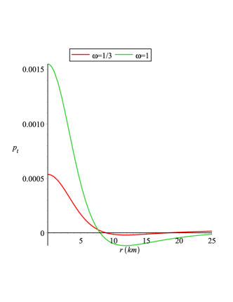
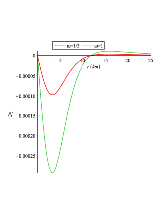
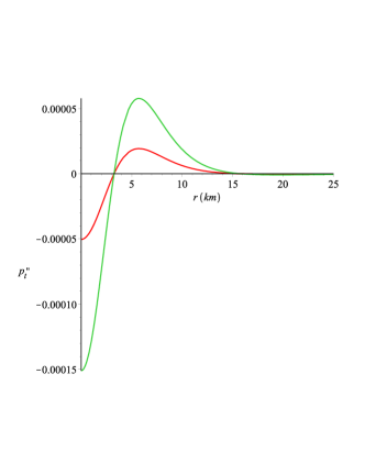
Fig. 3 : Variation of the $p_{t}$ (upper left), $p_{t}^{{}^{\prime}}$ (upper right) and $p_{t}^{{}^{\prime\prime}}$ (lower) with $r$

Form Fig. 3 it can be seen that the tangential pressure decreases with the radius and attain a minimum value which then again increases. This clearly indicates about pulsating nature of the compact star.

The central density is given by

$$\rho(0)=\frac{1}{2\pi}\left[\frac{(a-1)}{R^{2}}-\Lambda\right].$$ (22)

The central radial pressure is given by

$$p_{r}(0)=\omega\left(\frac{1}{2\pi}\left[\frac{(a-1)}{R^{2}}-\Lambda\right]\right)=\omega\rho(0).$$ (23)

The central tangential pressure is given by

$$p_{t}(0)=\frac{1}{2\pi R^{2}}(A-B)+\frac{\Lambda}{2\pi}.$$ (24)

From the above expressions we note that both the central density and central pressure are finite at the center of the star. So the present model is free from any central singularity.

4 Matching Condition

The exterior ($p=\rho=0$) solution corresponds to a static, BTZ-type black hole is written in the following form as

$$ds^{2}=-\left(-M_{0}-\Lambda r^{2}\right)dt^{2}+\left(-M_{0}-\Lambda r^{2}\right)^{-1}dr^{2}$$

$$+r^{2}d\theta^{2},$$ (25)

where $M_{0}$ is the conserved mass of the black hole which is associated with asymptotic invariance under time-displacements. Here we match the interior spacetime to the BTZ exterior at the boundary outside the event horizon. Continuity of the metric functions $g_{tt}$ and $g_{rr}$ at $r=b$, radius of the compact star, gives the value of the integration constant of Eq. (14) as

$$D=\frac{1}{2}(\omega+1)\left[\ln\left(\frac{R^{2}+b^{2}}{R^{2}+ab^{2}}\right)+\Lambda(ab^{2}-R^{2}\ln a)\right].$$ (26)

Putting $\omega=1/3$ we get the value of integration constant as $D=-0.5638$ and for $\omega=1$ it yields as $D=-0.8457$.

5 Physical Analysis

5.1 Anisotropic Behavior

For the model under consideration the measure of anisotropy in pressure can be obtained as

$$\Delta\equiv(p_{t}-p_{r}).$$ (27)

It can be seen that the ’anisotropy’ will be directed outward when $p_{t}>p_{r}$ i.e. $\Delta>0$ and inward when $p_{t}<p_{r}$ i.e. $\Delta<0$.

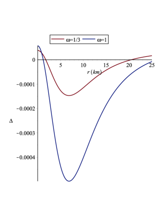
Fig. 4 : Variation of the anisotropic factor $\Delta$ with $r$

The profile of $\Delta$ with the radial distance is shown in Fig. 4. From this figure it is clear that the anisotropic factor does not vanish at the center of the star. It is positive from $1$ km (for $\omega=1$) to $2$ km (for $\omega=1/3$) i.e. $p_{t}>p_{r}$. This implies anisotropy is repulsive. Again for $\omega=1$ the anisotropic factor is negative between $1$ km to $25$ km and for $\omega=1/3$ the anisotropic factor is negative between $2$ km to $20$ km. After that $\Delta$ again increases to positive value. Since for the maximum part of the stellar distribution the anisotropy is negative so this allows construction of a more massive stellar structure as shown by Ray et al. (2012).

5.2 Energy Condition

For an anisotropic fluid sphere the energy conditions, viz. Weak Energy Condition (WEC), Null Energy Condition (NEC), Strong Energy Condition (SEC) and Dominant Energy Condition (DEC) are satisfied if and only if the following inequalities hold simultaneously by every points inside the fluid sphere:

$NEC:\rho+p_{r}\geq 0$,

$WEC:\rho+p_{r}\geq 0,\rho>0$,

$SEC:\rho+p_{r}\geq 0,\rho+p_{r}+2p_{t}>0$,

$DEC:\rho>|{p_{r}}|,\rho>|{p_{t}}|$.

We have shown the above inequalities by the help of graphical representation.

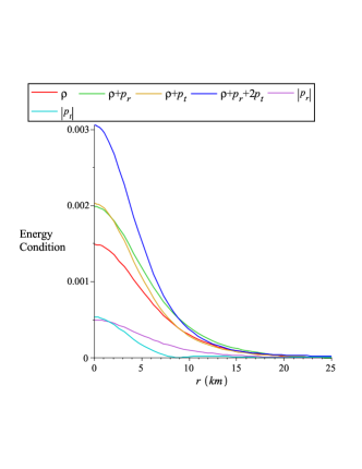
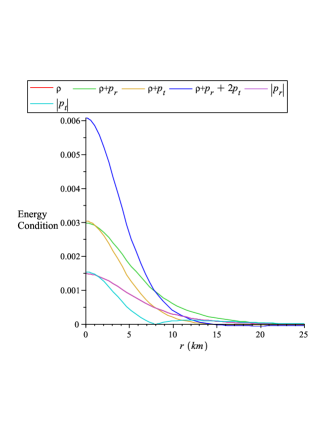
Fig. 5 : Variation of the Energy Condition against $r$ for $\omega=\frac{1}{3}$ (left panel) and $\omega=1$(right panel)

Fig. 5 shows the energy condition for $\omega=1/3$ (left panel). In this representation all the energy conditions are satisfied for our model. On the other hand, right panel of Fig. 5 shows the variation for $\omega=1$. This variation also shows that our model is satisfied for all the energy condition and our model provides a stable stellar configuration. However, as the graphs for $\rho$ and $p_{r}$ do overlap so we observe only five graphs.

5.3 Stability

The velocity of sound should follow the condition $0<v_{s}^{2}=dp/d\rho<1$ for a physically realistic model (Herrera, 1992; Abreu et al., 2007; Karar et al., 2012). This condition is known as causality condition. For our anisotropic model, the radial and transverse velocities of sound are defined by

$$v_{rs}^{2}=\frac{dp_{r}}{d\rho}=\omega,$$ (28)

$$v_{ts}^{2}=\frac{dp_{t}}{d\rho}.$$ (29)

Due to the mathematical complexity of the expression for $v_{ts}^{2}$ we shall show the inequality with the help of graphical representation only.

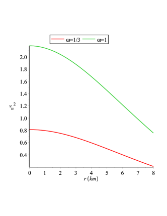
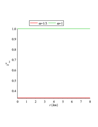
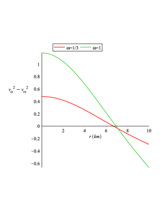
Fig. 6 : Variation of the transverse sound velocity $v_{ts}^{2}$ (upper left), radial sound velocity $v_{rs}^{2}$ (upper right) and $v_{ts}^{2}-v_{rs}^{2}$ (lower) with $r$

The variation of $v_{ts}^{2}$, $v_{rs}^{2}$ and $v_{ts}^{2}-v_{rs}^{2}$ with the radial distance $r$ are shown in Fig. 6. Herrera proposed a technique for stability check of local anisotropic matter distribution. This technique is known as the cracking concept which states that the region for which radial speed of sound is greater than the transverse speed of sound is a potentially stable region. Fig. 6 indicates that there is a change of sign for the term $v_{ts}^{2}-v_{rs}^{2}$ within the specific configuration and thus confirming that the model has a transition from unstable to stable configuration. The present stellar model gradually gets stability with the increase of the radius.

5.4 Buchdahl condition

The mass of the compact star can be calculated from the density profile

$$m(r)=\int 4\pi r^{\prime 2}\rho dr$$

$$=2R^{2}(a-1)\left[-\frac{r}{2a(R^{2}+ar^{2})}\right.$$

$$\left.+\frac{\arctan(\frac{\sqrt{a}r}{R})}{2a^{\frac{3}{2}}R}\right]-\frac{2\Lambda r^{3}}{3}.$$ (30)

Now the mass function is regular at the origin as $r\rightarrow 0$ $m(r)\rightarrow 0$. The profile of mass function is depicted in Fig. 7. From this figure it is clear that the mass function is monotonic increasing function of r and for $0\leq r\leq b$ $m(r)>0$.

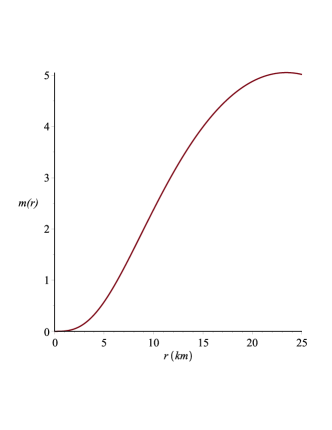
Fig. 7 : variation of the mass $m(r)$ with the radial distance $r$

The maximum allowable ratio of the mass to the radius of a compact star can not be arbitrarily large. According to Buchdahl (1959) the ratio of twice the maximum allowable mass to the radius is less than $8/9$, i.e. $2M/R<8/9$ where $M/R$ is called the compactification factor which classifies the stellar objects in different categories as given by Jotania and Tikekar (2006) as follows: (i) For normal star $M/R\sim 10^{-5}$, (ii) For white dwarf $M/R\sim 10^{-3}$, (iii) For neutron star $10^{-1}<M/R<1/4$, (iv) For ultracompact star $1/4<M/R<1/2$ and (v) For black hole $M/R=1/2$.

The compactification factor of our model is given by

$$u(r) = \frac{m(r)}{r}$$

$$= \frac{R(a-1)\arctan(\frac{\sqrt{a}r}{R})}{a^{\frac{3}{2}}r}-\frac{R^{2}(a-1)}{a(R^{2}+ar^{2})}-\frac{2\Lambda r^{2}}{3}.$$

(31)

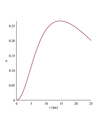
Fig. 8 : Variation of the compactification factor $u$ with the radial distance $r$

The variation of the mass and compactification factor with the radius of the star are shown in Figs. 7 and 8 respectively both of which are monotonic increasing function of $r$. Specifically, from the range of the compactification factor with its maximum value $>0.25$ of Fig. 8 we can conclude that our model of anisotropic star is an ultracompact star. We also calculate the redshift of our model

$$Z_{s}=(1-2u)^{-\frac{1}{2}}-1$$

$$=\left[1-\frac{2R(a-1)\arctan(\frac{\sqrt{a}r}{R})}{a^{\frac{3}{2}}r}\right.$$

$$\left.\qquad+\frac{2R^{2}(a-1)}{a(R^{2}+ar^{2})}+\frac{4\Lambda r^{2}}{3}\right]^{-\frac{1}{2}}-1.$$ (32)

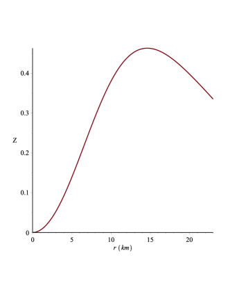
Fig. 9 : Variation of the redshift $Z$ with the radial distance $r$

The profile of the redshift function of our compact star is shown in Fig. 9. In this connection we want to mention that for anisotropic star the value of the maximum surface redshift for our model is near about $0.3$.

6 Concluding remarks

We have studied in the present work a $(2+1)$ dimensional compact star in the pseudo spheroidal spacetime. The motivation behind the study is the consideration that (i) the three-dimensional black holes are interesting by themselves, and (ii) the toy models in $3D$ may have a radically different qualitative behavior with respect to the more realistic $4D$ setups. Under this background we have studied the interior solution of a $(2+1)$ dimensional compact star in the pseudo spheroidal spacetime. The main guideline used in this work is a metric found in the Ref. (Vaidya and Tikekar, 1982), where a spheroidal 3-space exhibits central symmetry. It is clear that the investigation of the field of spheroidal bodies in general relativity has important astrophysical consequences, due to the fact the rotation of planets and stars produce spheroidal shapes. So, it seems that is a good approximation (slow rotation) to consider an static spheroidal spacetime to represent the gravitational field of these celescial bodies.

Therefore in the present work the Vaidya-Tikekar prescription (Vaidya and Tikekar, 1982) has been employed to get the matter density, radial pressure and other quantities from the Einstein field equations. Some salient and interesting features of the study can be put forward as follows:

(1) The matter density and radial pressure both are regular at the center and are monotonic decreasing function of the radial parameter. This behavior indicate that they have maximum value at the center and it decreases from the center to the boundary of the star. At the boundary of the star the radial pressure and matter density do vanish as expected.

(2) The tangential pressure is also a decreasing function of the radial distance. It decreases rapidly and within the stellar structure it has a fluctuating nature.

(3) The metric functions $g_{rr}$ and $g_{tt}$ are continuous at the boundary of the star. From this situation one can calculate the value of integration constant $D$.

(4) It is well known that the anisotropic factor $\triangle$ should vanish at the origin but our model does not show this feature rather it has a finite positive value. However, for the maximum part of our stellar distribution the anisotropy is repulsive which allows formation of more massive star.

(5) Our model satisfies all the energy conditions for $\omega=1/3$ and $\omega=1$. So our model provides a stable stellar configuration.

(6) We observe that by obeying Herrera’s cracking condition our model maintains stabilty with increase of the radius.

(7) The mass, compactification factor and surface redshift all are monotonic increasing function of the radius of the star. The maximum value of the compactification factor indicates that our model represents an ultra compact object. The maximum value of the surface redshift is about $0.3$ for the present model.

Finally, we would like to made some comments on our toy models in 3-dimension relative to the 4-dimensional one. As mentioned earlier, it seems that the 3D may have a radically different qualitative behavior with respect to the 4D having a more realistic setups. In connection to this it is to be noted that we have used the data from a 3-spatial dimensional object in order to estimate the constants of the model. Even though one can not have a strong argument about the physical meaning of the consideration of stellar objects of 2-spatial dimensions, however, for an observer in the plane, $\theta=constant$, all characteristics will reveal as a $(2+1)$ dimensional portrait. So superficially it will be more or less justified to use all the data which are apparently the same for both the spacetime. However, regarding development of a valid approach to represent lower dimensional gravity with spheroidal shapes one may follow the methodology of the Refs. (Quevedo, 1989; Chifu, 2012) for further investigation.

References

- Abreu et al. (2007) Abreu, H., Hernandez, H., Nunez, L. A.: Class. Quantum Gravit. 24, 4631 (2007)
- Banados et al. (1992) Baados, M., Teitelboim, C., Zanelli, J.: Phys. Rev. Lett. 69, 1849 (1992)
- Buchdahl (1959) Buchdahl, H.A.: Phys. Rev 116, 1027 (1959)
- Chattopadhyay et al. (2012) Chattopadhyay, P., Deb, R., Paul, B.C.: Int. J. Mod. Phys. D 21, 1250071 (2012)
- Chifu (2012) Chifu, E.N.: Abra. Zelm. J. 5, 31 (2012)
- Cruz and Zanelli (1995) Cruz, N., Zanelli, J.: Class. Quantum Gravit. 12, 975 (1995)
- Cruz et al. (2005) Cruz, N., Olivares, M., Villanueva, J.R.: Gen. Relativ. Gravit. 37, 667 (2005)
- Herrera (1992) Herrera, L.: Phys. Lett. A 165, 206 (1992)
- Hewish et al. (1968) Hewish, A., Bell, S. J., Pilkington, J.D.H., Scott, P.F., Collins, R.A.: Nature 217, 709 (1968)
- Husain (1995) Husain, V.: CGPG-95/10-8
- Jotania and Tikekar (2005) Jotania, K., Tikekar, R.: Int. J. Mod. Phys. D 14, 1037 (2005)
- Jotania and Tikekar (2006) Jotania, K., Tikekar, R.: Int. J. Mod. Phys. D 8, 1175 (2006)
- Kalam et al. (2012) Kalam, M., Rahaman, F., Ray, S., Hossein, M., Karar, I., Naskar, J.: Euro. Phys. J. C. 72, 2248 (2012)
- Karar et al. (2012) Karar, I., Rahaman, F., Sharma, R., Ray, S.: Euro. Phys. J. C. 72, 2071 (2012)
- Knutsen (1988) Knutsen, H.: Mon. Not. Roy. Astron. Soc. 232, 163 (1988)
- Maharaja and Leach (1996) Maharaja, S.D., Leach, P.G.L.: J. Math. Phys. 37, 430 (1996)
- Mann and Ross (1993) Mann, R.B., Ross, S.F.: Phys Rev D 47, 3319 (1993)
- Martins et al. (2010) Martins, M.R., Da Silva, M.F.A., Sheng, A.D.: Gen. Relativ. Gravit. 42, 281 (2010)
- Patel and Mehta (1995) Patel, L.K., Mehta, N.P.: Aust. J. Phys. 48, 635 (1995)
- Paulo (1999) Paulo, M.S.: Phys. Lett. B 467, 40 (1999)
- Quevedo (1989) Quevedo, H.: Phys. Rev. D 39, 2904 (1989)
- Ray et al. (2012) Ray, S., Hossain, M., Rahaman, F., Naskar, J., Kalam, M.: Int. J. Mod. Phys. D 21, 1250088 (2012)
- Rhodes and Ruffini (1974) Rhodes, C.E., Ruffini, R.: Phys. Rev. Lett. 32, 324 (1974)
- Ruderman (1972) Ruderman, R.: Rev. Astr. Astrophys. 10, 427 (1972)
- Sharma et al. (2011) Sharma, R., Rahaman, F., Karar, I.: Phys. Lett. B 704, 1 (2011)
- Shee et al. (2016) Shee, D., Rahaman, F., Guha, B.K., Ray, S.: Astrophys. Space Sci. 167, 361 (2016)
- Thirukkanesh and Ragel (2014) Thirukkanesh, S., Ragel, F.C.: Astrophys. Space Sci. 352, 743 (2014)
- Thomas and Tikekar (1998) Thomas, V.O., Tikekar, R.: Pramana-J. Phys. 50, 95 (1998)
- Tikekar (1990) Tikekar, R.: J. Math Phys. 31, 2454 (1990)
- Tikekar and Thomas (1999) Tikekar, R., Thomas, V.O.: Pramana-J. Phys. 52, 237 (1999)
- Vaidya and Tikekar (1982) Vaidya, P.C., Tikekar, R.: J. Astrophysics. Astron. 3, 325 (1982)