Time evolution of Hanle and Zeeman polarization in MHD models

Abstract

Exposing the polarization signatures of the solar chromosphere requires studying its temporal variations, which is rarely done when modelling and interpreting scattering and Hanle signals. The present contribution sketches the scientific problem of solar polarization diagnosis from the point of view of the temporal dimension, remarking some key aspects for solving it. Our time-dependent calculations expose the need of considering dynamics explicitly when modelling and observing scattering polarization in order to achieve effective diagnosis techniques as well as a deeper knowledge of the second solar spectrum.

1 Introduction

Understanding the scattering polarization generated by a stellar atmosphere in Non-LTE depends on how accurately is the temporal evolution considered. An example of the central role of time in such a context is the mere fact that the radiative transfer equation (RTE) and the rate equations for polarized light result from applying the Schr dinger equation to the time-evolution operator (Landi Degl’Innocenti 1983; Bommier 1997). In the solar case, time evolution plays a role over a huge range of scales (see Fig. 2). The smallest time scales, between $10^{-14}$ and $1$ s, are associated to quantum processes of interaction between matter and matter (collisions), matter and radiation (absorption and emission), and matter and magnetic field (Hanle and Zeeman effects), either with atoms that preserve partial temporal memory of the incident light during scattering (partial redistribution, PRD) or that do not (CRD). In medium scales ($10^{-2}<\Delta\rm t(s)<10^{2}$), the response of the detectors is critical, particularly in terms of temporal integration, and of management of noise sources (seeing, readout, shot, thermal) peaking at different characteristic times during detection. Finally, in scales $>10$ s, chromospheric motions have a key impact in the generation and transfer of polarized light.

The temporal perspective of the aforementioned processes suggests that their very different time-scales can decouple them, allowing a division in smaller subproblems. Thus, an explicit care of the temporal dimension is substituted by generally good approximations that are universally adopted (e.g., statistical equilibrium). However, when processes overlapping in time are modelled separately, or when a quantity is not well resolved, inconsistencies and paradoxes may occur. A trivial example of this is the integration of chromospheric dynamic signals whose characteristic time scales are significantly shorter than the integration time. If in addition chromospheric polarization is modelled in absence of temporal evolution, the theoretical predictions change radically. Recently, Carlin & Bianda (2016) investigated these issues by carrying out the first detailed simulation of temporal evolution of Hanle and Zeeman polarization, done for the Ca i $4227$ Å line with help of chromospheric MHD models (Carlsson et al. 2016). For more details on the calculations, see Carlin et al. (2017, submitted). Next sections provide some contextual explanations and illustrative results.

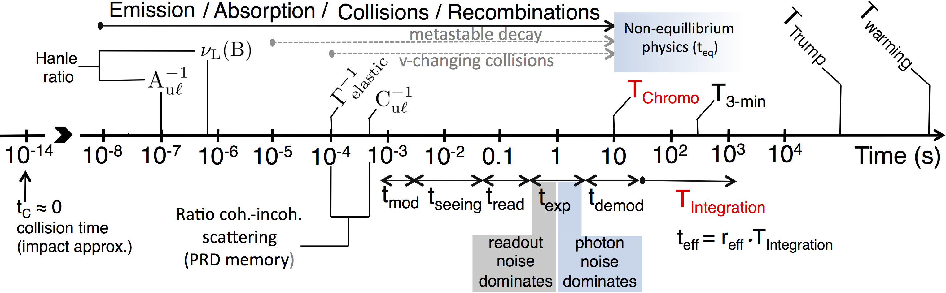
Figure 1.: Temporal scales explaining chromospheric Non-LTE polarization .

2 Theoretical considerations about dynamics

The solution of the Non-LTE RT problem with atomic polarization implies to calculate the optical properties of the plasma. This is done by solving the rate equations, which describe the evolution of the atomic density matrix $\rho^{K}_{Q,\mathrm{i}}$ in each atomic level $i$ considered (Landi Degl’Innocenti & Landolfi 2004). Symbolically, the comoving-frame rate equations for a plasma element 0 moving with velocity $\vec{\upsilon}_{\mathrm{macro}}$ are of the kind:

$$\centering\frac{\partial\rho^{K}_{Q,i}}{\partial t}+\vec{\upsilon}_{\rm macro}\cdot\vec{\nabla}\left[\rho^{K}_{Q,i}\right]=\,f^{\nu_{L}}_{B}\left(\vec{B},\rho^{K}_{Q,i^{\prime}}\right)+f^{A_{u\ell}}_{\rm rad}\left(J^{K}_{Q},\rho^{K}_{Q,i^{\prime}}\right)+f^{C_{ii^{\prime}}}_{\rm col}\left(n,T,\rho^{K}_{Q,i^{\prime}}\right)\@add@centering$$ (1)

Here, the total temporal variation of the atomic collectivity in 0 has magnetic ($f_{\rm B}$), radiative ($f_{\rm rad}$) and collisional ($f_{\rm col}$) contributions whose maximum values have representative orders of magnitude given by the Larmor frequency ($\nu_{L}$), the Einstein coefficient $A_{u\ell}$ and the collisional rates ($C_{ii^{\prime}}$), respectively. In addition, such contributions change with time due to the MHD quantities ($\vec{\rm B}$, $\vec{\upsilon}_{\rm macro}$, T, n) and to the radiation field tensor J${}^{K}_{Q}$. As the atomic rates are far larger than the temporal variations due to macroscopic quantities, the partial temporal derivative in Eq.(1) is relatively large and controlled by atomic processes. Furthermore, the second term of the l.h.s. can be disregarded against the time derivative, namely when the amount of net $\rho^{K}_{Q,i}$ introduced in the plasma element at speed $\upsilon_{\rm{macro}}$ is negligible. In this situation, the atomic collectivity reaches statistical equilibrium quickly. Hence, Eq.(1) is usually solved by forcing the temporal derivative to zero and neglecting the spatial derivative (statistical equilibrium equation, SEE). This way, the atmosphere is considered stationary at intermediate time scales, the time step being assumed large enough to reach equilibrium ($\rm\Delta t>>t_{eq}$) but short enough to avoid significant net flow of material in the volume considered ($\rm\Delta t<<t_{mat}$). The first condition is satisfied in our calculations for Ca i $\lambda 4227$ but it might fail in some atomic systems with long-lived metastable levels. The second condition has been assumed as valid in the present work but in chromospheric shock fronts the possible values of velocity, atomic polarization, density and collisions pose doubts requiring further investigation.

Macroscopic dynamics is clearly key in the RTE. In a planar time-dependent stellar atmosphere with non-relativistic macroscopic speeds, the general RTE for the Stokes vector ${\bf\rm{I}}^{0}(\vec{\Omega},x^{0},s,t)=\rm(I,Q,U,V)^{\rm{T}}$ in a reference frame comoving with 0 is

$$\centering\frac{1}{c}\frac{\partial\rm{\bf{I}}^{0}}{\partial t}+\frac{\partial\rm{\bf{I}}^{0}}{\partial s}-\frac{\rm{d}\mathcal{V}}{\rm{d}s}\frac{\partial\rm{\bf{I}}^{0}}{\partial x^{0}}={\mathbf{\epsilon}}^{0}-{\bf K}^{0}\rm{\bf{I}}^{0},\qquad\textrm{}\@add@centering$$ (2)

where all the symbols have standard meaning and $\mathcal{V}(s)=\vec{\xi}\cdot\vec{\Omega}$ is the projection along ray $\vec{\Omega}$ of the macroscopic Doppler velocity $\vec{\xi}$ (always in Doppler units at 0). Namely, $\xi=\upsilon_{\rm{macro}}/(\upsilon^{0}_{\rm{thermal}}+\upsilon^{0}_{\rm{turb}})^{1/2}$ is a ratio between resolved and unresolved velocities. Eq. (2) shows succinctly that the emergent solar polarization depends on three very important points: (i) the spectral structure of the radiation field seen from the scatterers ($\partial\rm{I^{0}}/\partial x^{0}$), (ii) the gradients of macroscopic motions ($\rm{d\mathcal{V}/\rm{ds}}$) modulating such an incident field, and (iii) its temporal variation ($\partial\rm{I^{0}}/\partial t$). In the comoving frame (CMF) RTE, macroscopic motions only appear in an explicit dedicated term (third one in the l.h.s.), with no role anywhere else. Thus, such a CMF term is more sensitive to $\upsilon_{\rm{macro}}$ when the plasma is cooler ($\upsilon^{0}_{\rm{thermal}}\downarrow$), but vanishes when $\upsilon_{\rm{macro}}$ is constant or unresolved. It also shows that assuming $\mathcal{V}\propto\mu\cdot\upsilon_{z}/\upsilon^{0}_{\rm{thermal}}$, as implicit when realistic models are treated in $1.5$D, just implies that vertical velocity gradients are assumed much stronger than horizontal ones. This describes a quiet chromosphere where weak magnetic fields cannot guide shock waves or gravity-accelerated flows towards the horizontal. In compliance with the dominance of vertical variations, $1.5$D calculations as ours consider an azimuthally-independent radiation field, instead of the more general one affected by horizontal inhomogeneities (e.g., Štěpán & Trujillo Bueno 2016).

Note also that the l.h.s. of Eq. (2) is valid in uniform motion (Mihalas 1978): the acceleration of 0 between timesteps must be significantly smaller than the relative velocity between adjacent plasma elements. This seems fulfilled in chromospheric models, also in shock waves. Finally, the temporal variation can be treated implicitly by solving the whole problem independently for each snapshot of the MHD simulation, which implies the very good approximation $c^{-1}\partial{\bf I}/\partial t=0$.

The solution to Eq. (2) for each ray and point in the atmospheric volume is ${\bf\rm{I}}^{0}(\vec{\Omega},x^{0},s,t)$. Such radiation field is shaped angularly by Doppler shifts along rays connecting each location with the scatterer $0$. Thus, chromospheric motions can efficiently generate anisotropic radiation that modulates the polarization properties of the plasma and the emergent Stokes vector in short temporal scales (Carlin et al. 2013).

$\begin{array}[]{cc}\includegraphics[scale={0.45}]{carlin_1_fig2a.png}&\includegraphics[scale={0.45}]{carlin_1_fig2b.png}\end{array}$

Figure 2.: Poincar diagrams in (static) semiempirical FALC models for ad-hoc B$=10$ G (left) and B$=120$ G (right) in $\mu=1$. In black: some lines of $\rm\chi_{B}=cte$.

3 Poincar diagrams and Hanle effect in static models

Before considering dynamic signals it is useful to characterize the Hanle and Zeeman effects for the given spectral line. To do it, we propose to represent the polarization in the space Q,U,V (Poincar diagram), as in the Figure 2.

In Ca i $4227$ Å, the upper-level Hanle critical field is $\approx 20$-$25$ G, which implies Hanle sensitivity to magnetic fields between $5$ and $125$ G. Figure 2 shows two main effects of increasing the magnetic strength in that range at disk center. The first one is the progressive cancellation of the linear polarization (LP) as the magnetic field inclination $\theta_{\rm B}\rightarrow 54^{\rm o},125^{\rm o}$ (Van-Vleck angles). This effect is maximum in full Hanle saturation (right panel) and can produce Hanle polarity inversion lines (HPIL, Carlin & Asensio Ramos 2015) in synthetic maps of scattering polarization. Calculating for other field strengths we find that Van-Vleck HPILs are already quiet developed (LP<LP^max/4) for B$\geq 60$ G, hence full Hanle saturation is not necessary to create such features in a spatial map. Poincar diagrams reveal a second interesting aspect of the forward-scattering Hanle effect. A same magnetic field azimuth produces different U/Q ratios depending on the magnetic field inclination. Then, the spectropolarimetric azimuth can be estimated (also out of saturation) with $\rm\tan\chi_{B}=\,$U/Q if subtracting an inclination-dependent magnetic field azimuth offset given by V/I (see forthcoming paper).

$\begin{array}[]{c}\includegraphics[scale={0.93}]{carlin_1_fig3a.png}\\ \includegraphics[scale={0.75}]{carlin_1_fig3b.png}\end{array}$

Figure 3.: Time serie in one pixel of the slit. Upper panel: real parts of $\rho^{2}_{1}$ and $\rho^{2}_{2}$ (lambdafied at 1), Q/I and U/I Hanle, V/I, $10\times$Q/I and $10\times$U/I Zeeman. Lower panel: lambdification at $1$ of atmospheric quantities. $\rm w_{20}$ is radiation field anisotropy.

$\begin{array}[]{cc}\includegraphics[scale={0.55}]{carlin_1_fig4a.png}&\includegraphics[scale={0.5}]{carlin_1_fig4b.png}\end{array}$

Figure 4.: Left: synthetic slit profiles in $\rm t=7.8$ min (after integrating the width of the slit). Right: dependence of the maximum total LP (percentile 99.5%) on resolution ($\rm\Delta x$,$\rm\Delta t$).

4 The dynamic Hanle effect of Ca I 4227Å

To analyze the temporal evolution, the transformation lambdafy M at $\alpha$ is defined as $\rm M_{xy}(z,t)\rightarrow M_{x,y}(\lambda_{\tau=\alpha},t)$. Thus is how Fig. 3 associates quantities at $\tau(\lambda)=1$ with Stokes profiles in $\lambda$. The figure shows the temporal evolution of synthetic Hanle and Zeeman polarization in one pixel at quiet sun for $\lambda 4227$. Note the much weaker transversal Zeeman, the interesting spectral variability (symmetries, shifts) and the amplitudes of the Hanle LP along time. A reason for the large LP amplitudes is that the magnetic strength and inclination vary close to values ($\theta_{B}=90,\,B\approx 22$G) maximizing the forward-scattering Hanle effect in the chromospheric line core (see Figs.2 and 3). Additionally, the LP is substantially larger than in observations because the spatio-temporal resolution is increased, hence also the effect of the parameter $\xi$ introduced in Eq.(2) and controlling the LP amplitudes through velocity gradients and radiation field anisotropy, as explained in Carlin et al. (2012). Indeed, time integration can reduce the LP substantially, as seen in Fig.4, where the response of the maximum LP values in our synthetic slit is shown for different resolutions. Furthermore, it was found that the spectral variability combined with integrations larger than $3$ minutes changes completely the morphology of the signals. As these modulation effects are line dependent, Carlin & Bianda (2016) have pointed out that temporal evolution/integration with macroscopic motions can account for the anomalous excesses of line-core LP in the second solar spectrum that have puzzled our community for years (Stenflo et al. 2000).

Unfortunately, measuring time evolution is hard. A decent S/N usually implies time integration because solar scattering polarization is weak (hence noisy). But our results show that part of that weakness might be due to a combination of dynamic issues (Carlin & Bianda 2016). One of them is the lack of temporal resolution, which partially cancels the LP because the latter can change of sign in a single profile as well as between close timesteps and pixels. Thus, at non-full resolutions, cancellation makes LP more sensitive to noise and even longer integrations seem necessary. But, what happens when a sensitive spectropolarimeter is combined with a full resolution avoiding cancellations?

Observations with the ZIMPOL camera (Ramelli et al. 2010) having poor spatial resolution ($0.^{\prime\prime}6-1.^{\prime\prime}4$), good temporal resolution ($\rm t_{integ}<30$ s) and medium effective integration ratio ($\rm r_{eff}=t_{eff}/t_{integ}\approx 0.55$) give large noisy signals. Therefore, the amplitude that might have been gained by resolving in time the LP (and its enhancements produced by motions) is not enough against the intrinsic noise at such poor spatial resolution and medium effective integration time. What are the keys for going further? First, the instrumental time scales (see Fig. 2). While $\rm t_{integ}$ has to be minimized, the net temporal integration $\rm t_{eff}$ has to be maximized (larger $\rm r_{eff}$), which is limited by the readout time of the camera and by the exposure time ($\rm t_{exp}$) that saturates the pixel in intensity. The second key is noise management. The design maximizing $\rm r_{eff}$ (e.g., higher sampling/shorter $\rm t_{exp}$ or viceversa) needs also to consider and reduce the kind of noise dominating during exposure time. The existence of detection suggests that photon noise dominates in our case (thermal noise is not a problem in the violet for cooled CCDs). Finally, full spatial resolution is required, meaning a large telescope with a stabilization system working in on-disk quiet-sun, which is also very challenging.

In summary, measuring polarization in chromospheric scales requires well-known solutions: (i) minimize noise, by increasing the detected intensity with larger telescope apertures and efficiencies, by maximizing the net temporal integration, and by a suited lower-noise camera design. And (ii), increase spatiotemporal resolution, again with large telescopes and by optimizing the temporal processes in the camera. The achievement of top spatio-temporal resolution ($<15$ s, $<0.2^{\prime\prime}$) should expose intrinsically larger LP Hanle signals by avoiding cancellations (at least in $\lambda 4227$), hence improving our ability to discern the real (time-resolved) second solar spectrum.

5 Conclusions

Temporal evolution is key for a true understanding of the second solar spectrum and for diagnosing chromospheric magnetic fields. First, because morphological (spectral) information is lost without it, but also because temporal resolution itself avoids spectral cancellations that Hanle polarization might be prone to suffer in moving media. Thus, LP amplitudes can increase, and magnetic fingerprints encoded in null-polarization lines (Hanle PILs, see Sec.3) might be more easily detected by spatial contrast.

Consequently, the modelling of polarization should consider dynamics (time evolution and macroscopic motions) when possible. Further investigation is needed for assessing how important are the streaming terms in the SEE and the subsequent possible lack of statistical equilibrium in shock waves.

On the other hand, Hanle time series at chromospheric time scales demand large telescopes and/or an exquisite management of noise and temporal efficiency in the spectropolarimeter. These challenges require more research and technological advances, but they are key (and achievable) steps for providing with effective Hanle diagnosis techniques to the solar community.

Acknowledgments

The author thanks Michele Bianda, Daniel Gisler and Renzo Ramelli for their support and feedback in regard to observational and instrumental matters. This work was financed by the SERI project C12.0084 (COST action MP1104) and by the Swiss National Science Foundation project $200021$_$163405$.

References

- Bommier (1997) Bommier, V. 1997, A&A, 328, 706
- Carlin & Asensio Ramos (2015) Carlin, E. S., & Asensio Ramos, A. 2015, ApJ, 801, 16
- Carlin et al. (2013) Carlin, E. S., Asensio Ramos, A., & Trujillo Bueno, J. 2013, ApJ, 764, 40.
- Carlin & Bianda (2016) Carlin, E. S., & Bianda, M. 2016, ApJL, 831, L5
- Carlin et al. (2012) Carlin, E. S., Manso Sainz, R., Asensio Ramos, A., & Trujillo Bueno, J. 2012, ApJ, 751, 5.
- Carlsson et al. (2016) Carlsson, M., Hansteen, V. H., Gudiksen, B. V., Leenaarts, J., & De Pontieu, B. 2016, A&A, 585, A4.
- Landi Degl’Innocenti (1983) Landi Degl’Innocenti, E. 1983, Sol. Phys., 85, 3
- Landi Degl’Innocenti & Landolfi (2004) Landi Degl’Innocenti, E., & Landolfi, M. 2004, Polarization in Spectral Lines (Kluwer Academic Publishers)
- Mihalas (1978) Mihalas, D. 1978, in Stellar Atmospheres, vol. 455
- Ramelli et al. (2010) Ramelli, R., Balemi, S., Bianda, M., Defilippis, I., Gamma, L., Hagenbuch, S., Rogantini, M., Steiner, P., & Stenflo, J. O. 2010, SPIE, 77351Y.
- Stenflo et al. (2000) Stenflo, J. O., Gandorfer, A., & Keller, C. U. 2000, A&A, 355, 781
- Štěpán & Trujillo Bueno (2016) Štěpán, J., & Trujillo Bueno, J. 2016, ApJL, 826, L10.