Probing the primordial universe with gravitational waves detectors

Abstract

The spectrum of primordial gravitational waves (GWs), especially its tilt $n_{T}$, carries significant information about the primordial universe. Combining recent aLIGO and Planck2015+BK14 data, we find that the current limit is $n_{T}=0.016^{+0.614}_{-0.989}$ at 95% C.L. We also estimate the impacts of Einstein Telescope and LISA on constraining $n_{T}$. Moreover, based on the effective field theory of cosmological perturbations, we make an attempt to confront some models of early universe scenarios, which produce blue-tilted GWs spectrum ($n_{T}>0$), with the corresponding datasets.

I Introduction

In the recent years, searching for the primordial gravitational waves (GWs) [1, 2] has invigorated the cosmological community. Since the primordial GWs carry rich information about the early universe and the UV-complete gravity theory, its detection would deepen our understanding for the early universe scenario, see Refs.[3, 4, 5] for reviews.

The primordial GWs background, described mainly by its tilt $n_{T}$ and the amplitude $A_{T}=rA_{s}$ at the pivot scale $k_{*}$, spans a broad frequency-band, $10^{-18}-10^{10}$ Hz. The slow-roll inflation [6, 7] predicts a slightly red-tilted spectrum with $n_{T}\simeq-2\epsilon_{inf}<0$ and $0<\epsilon_{inf}\ll 1$. However, $n_{T}>0$ is interesting, since it boosts the primordial GWs background at the frequency-band of laser interferometers (Advanced LIGO/Virgo, as well as the space-based detectors), e.g.[8, 9].

The primordial GWs at ultra-low frequency $10^{-18}-10^{-16}$ Hz, or on large scale, may induce the B-mode polarization in the cosmological microwave background (CMB)[10, 11]. The joint analysis of BICEP2/Keck Array and Planck (BKP) data have put the constraint on the amplitude of primordial GWs, $r_{0.05}<0.12$ (95% C.L.) [12]. Recently, the combination of above data and Keck Array’s 95 GHz data have improved the constraint to $r_{0.05}<0.07$ (95% C.L.) [13] (BK14). However, no strong limit was found for the tilt $n_{T}$, which is because the CMB band is too narrow to depict the whole property of GWs background[14, 15].

Recently, the LIGO Scientific Collaboration, using ground-based laser interferometer, has observed a GW signal (GW150914) with a significance in excess of 5.1$\sigma$ [16], which is consistent with an event of the binary black hole coalescence based on general relativity (GR). Advanced LIGO (aLIGO) O1 put an upper limit for the stochastic GWs background at the frequency band $f\simeq 30\,{\rm Hz}$ [17, 18].

The spectrum of primordial GWs is not only determined by the evolution of the background in early universe scenarios, e.g.[19, 20], but also significantly affected by the modifications to GR. The Effective Field Theory (EFT) [21, 22, 23, 24, 25] of cosmological perturbations offers a unifying platform to deal with the cosmological perturbations of modified gravity theories, such as the Horndeski theory [26] and its beyond [27]. The EFT method has also been used in building healthy nonsingular cosmological models [28, 29]. Different models of early universe scenarios generally have different predictions for $n_{T}$. Only when the measurements at different frequency bands are combined, can one put tighter constraint on the tilt $n_{T}$ [30, 31, 32, 33, 34].

Therefore, it is interesting to perform a joint analysis of recent aLIGO O1 and Planck 2015+BK14 dataset to constrain $n_{T}$, as well as confront the EFT parameters in corresponding models with the data.

The planned space-based detector LISA will search the GWs signals at the frequency about 1 mHz [35, 36] collect data in 2030s, and recently LISA Pathfinder has been launched which paving the way for the LISA mission. While the space-based GWs detection project also has been approved in China. Moreover, the third generation ground-based detector, Einstein Telescope (ET) [37], is also being planned, which has higher sensitivity than aLIGO/VIRGO. Thus it will also be interesting to estimate the capability of LISA and ET in constraining the tilt $n_{T}$.

This paper is organized as follows. In Sec.II, combining recent aLIGO and Planck2015 +BK14 data, we provide an updated constraint on the tilt $n_{T}$ of primordial GWs, and also forecast the impacts of LISA and ET. In Sec.III, based on EFT, we explore how to confront the models of early universe scenarios, which produce blue-tilted GWs spectrum ($n_{T}>0$), with the corresponding datasets. Sec.IV is the conclusion.

II Method, results and forecasts

II.1 Upper limits put by interferometers

Conventionally, one define

$$\Omega_{\text{GW}}(k,\tau_{0})=\frac{1}{\rho_{\text{c}}}\frac{d\rho_{\text{GW}}}{d\ln k}=\frac{k^{2}}{12a_{0}^{2}H^{2}_{0}}P_{T}(k)T^{2}(k,\tau_{0})\,$$ (1)

to depict the relic GWs background, where $\rho_{\text{c}}=3H^{2}_{0}/\big{(}8\pi G\big{)}$ is the critical density, $\Omega_{GW}(k,\tau_{0})$ reflects the fraction of $\rho_{\text{GW}}$ per logarithmic $k$-interval, and $\rho_{\text{GW}}$ is the present energy density of GWs. The primordial GWs spectrum $P_{T}(k)$ is generally

$$P_{T}(k)=rA_{s}\left(\frac{k}{k_{*}}\right)^{n_{T}},\,$$ (2)

where $n_{T}$ is the tilt of spectrum, and $A_{s}$ is the amplitude of primordial scalar perturbations at the pivot scale $k_{*}$. When applying Eq.(2) to fit CMB data, usually one set $k_{*}=k_{CMB}\sim 0.01\,\mathrm{Mpc}^{-1}$. Current constraint put by CMB data is $r_{0.05}<0.07$ (95% C.L.) with $k_{*}=0.05\,\mathrm{Mpc}^{-1}$ [13] (BK14), which corresponds to $\Omega_{\text{GW}}<10^{-15}$ at $k\sim 10^{-16}$ Hz. Transfer function $T(k,\tau_{0})$ is [38, 39, 40, 41],

$$T(k,\tau_{0})=\frac{3\Omega_{\text{m}}j_{1}(k\tau_{0})}{k\tau_{0}}\sqrt{1.0+1.36\frac{k}{k_{\text{eq}}}+2.50\big{(}\frac{k}{k_{\text{eq}}})^{2}},$$ (3)

where $\Omega_{\text{m}}={\rho_{\text{m}}/\rho_{c}}$, see also [42].

Current upper bound put by aLIGO O1 is $\Omega_{\mathrm{GW}}<{10^{-7}}$ [17, 18] at the frequency $f\simeq 30\,{\rm Hz}$, in which the wavenumber $k$ is related to $f$ by $f={k}/{2\pi a_{0}}$. The network of aLIGO and Virgo detectors operating at their final observing runs O5 will be able to arrive at $\Omega_{\mathrm{GW}}\sim 10^{-9}$.

II.2 Combined datasets (interferometers and CMB) and results

The parameters set of the lensed-$\Lambda$CDM model is $\{\Omega_{b}h^{2},\Omega_{c}h^{2},100\theta_{\mathrm{MC}},\tau,\ln(10^{10}A_{s}),n_{s}\}$, with the baryon density $\Omega_{b}h^{2}$, the cold dark matter density $\Omega_{c}h^{2}$, the angular size $\theta_{\mathrm{MC}}$ of the sound horizon at decoupling, the reionization optical depth $\tau$, the amplitude $\ln(10^{10}A_{s})$ and the tilt $n_{s}$ of the primordial scalar perturbation spectrum. We also include the parameters $r=A_{T}/A_{s}$ and $n_{T}$, which satisfy (2). We use the pivot scale $k_{*}=0.01\,\mathrm{Mpc}^{-1}$.

We will apply the full set of the Planck 2015 likelihood in both temperature and polarization (referred as PlanckTT, TE, EE+lowTEB). The Planck likelihood [43] combined with the BICEP/Keck data [13] (BK14) will be used. In all runs, we also include a prior on the Hubble parameter from the HST [44] and BAO [45, 46, 47].

Our analysis of combining CMB and interferometers data will be computed based on the recent CMB data and the upper limits put by recent aLIGO O1 on stochastic GWs background $\Omega_{\mathrm{GW}}$. In order to perform such analysis, we add a module computing $\Omega_{\mathrm{GW}}$ into the CosmoMC [48] and the CAMB [49].

In Table.1, we list our best-fit results for the parameters set of the lensed-$\Lambda$CDM model $\{\Omega_{b}h^{2},\Omega_{c}h^{2},100\theta_{\mathrm{MC}},\tau,\ln(10^{10}A_{s}),n_{s}\}$. We see that considering the aLIGO O1 data does not significantly alter the results provided by CMB data. Intuitively, this result is because the GWs only contribute a small fraction of CMB fluctuations $r\ll 1$.

	$\bf All$	$\bf All+aLIGO$	$\bf All+LISA$	$\bf All+ET$
$\Omega_{b}h^{2}$	$0.022$	$0.022$	$0.022$	$0.022$
$\Omega_{c}h^{2}$	$0.119$	$0.119$	$0.119$	$0.118$
$100\theta_{\mathrm{MC}}$	$1.04$	$1.04$	$1.04$	$1.04$
$\tau$	$0.08$	$0.08$	$0.08$	$0.09$
$ln(10^{10}A_{s})$	$3.12$	$3.14$	$3.15$	$3.15$
$n_{s}$	$0.968$	$0.971$	$0.968$	$0.968$

Table 1: Summary of constraints on the cosmological 6-parameters set $\{\Omega_{b}h^{2},\Omega_{c}h^{2},100\theta_{\mathrm{MC}},\tau,\ln(10^{10}A_{s}),n_{s}\}$. “All” refers to Planck2015, HST, BAO and BK14 data.

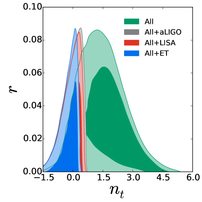
Figure 1: Marginalized posterior distributions at 68% and 95% C.L. for the parameters $r$ and $n_{T}$. “All” refers to Planck2015, HST, BAO and BK14 data.

However, the constraint on $r$ and $n_{T}$ will be affected importantly, which is plotted in Fig.1. Only CMB data is used, the posteriors for $n_{T}$ favor a blue tilt. When we consider the CMB+aLIGO O1 dataset, the upper limit for $n_{T}$ is cut by a big margin, since a large $n_{T}$ could bring a detectable GWs signal at small scales. The constraint result is presented in Table.2, in which $n_{T}=0.016^{+0.614}_{-0.989}$. Here, since $k_{*}$ in (2) is set around CMB scale, only the CMB data is sensitive to the GWs background with $n_{T}<0$.

In Ref.[32], Lasky et.al utilized LIGO S5 data collected in 2009-2010, see also [50]. In Ref.[31], Cabass et.al also performed a combined analysis of Planck2015+BK14 and aLIGO data. However, the aLIGO sensitivity they used is $\Omega_{\mathrm{GW}}\sim 10^{-9}$ at $f=100$ Hz, which only serves as a forecast, while the current result of aLIGO O1 is $\Omega_{\mathrm{GW}}\sim 10^{-8}$, see Sec.II.1. Thus we provide an updated limit on $n_{T}$ by using up-to-date CMB+aLIGO datasets.

II.3 Forecasts

In a slightly lower frequency-band, i.e. 1mHz, planning space-based detector LISA will possibly set $\Omega_{\mathrm{GW}}\sim 10^{-14}$ [5, 51]. The sensitivities of LISA’s different configurations are different. Here, we will use $\Omega_{\mathrm{GW}}<\rm{3.72\times 10^{-13}}$ at $f\simeq 3.8\times 10^{-3}$ Hz for our analysis. This upper limit get from the configuration N2A2M2L6, where N2 presents the best low-frequency noise level, A2 represents 2 millon kilometers arm length, 2-years duration of observation is represented by M2, and L6 corresponds to 6 links.

The ET is a proposed ground-based GWs detector, which belongs to the third generation detector. It is designed to consist of six Michelson interferometers, which form an equilateral triangle. The arm length will be reached $10$ kilometers long. The ET will possibly put the upper limit for stochastic GWs background to $\Omega_{\mathrm{GW}}<\rm{10^{-13}}$ at $f\simeq 10$ Hz [37, 52].

We consider the combinations of the CMB data and the upper limits put by the expected ET and LISA’s sensitivities. From the Table.1, we see that the expected ET and LISA’s sensitivities does not significantly alter the cosmological 6-parameters results provided by CMB data. yet the constraint on $r$ and $n_{T}$ is significantly, The forecast result of CMB+ET and CMB+LISA are also presented in Table.2, in which $n_{T}=-0.050^{+0.612}_{-0.992}$, $-0.184^{+0.534}_{-0.877}$ for above datasets, respectively. This indicates that the ground- and space-based interferometers are able to significantly improve the limits on the tilt $n_{T}$ of primordial GWs. In fact, besides these current ground- and space-based CMB observation, some other measurements can also give the constraint on $n_{t}$. In Ref.[53], Liu and Zhao et.al utilized PTA data to show $n_{t}$ upper limit, if $r=0.01$, the optimal gives limit $n_{t}<0.18$ .

As far as the forecasts are concerned, in 2020s the sensitivity of aLIGO/Virgo O5 will arrive at $\Omega_{\mathrm{GW}}\sim 10^{-9}$ [17]. However, it cannot improve the current limit on $n_{T}$ put by O1 well, and is still weaker than the limit provided by the future LISA, which will operate in 2030s, since at LISA frequency-band the sensitivity of O5 corresponds to $\Omega_{\mathrm{GW}}=(k_{LISA}/k_{aLIGO})^{n_{T}}\Omega_{\mathrm{GW}}^{aLIGO}\sim 10^{-10}$, which is still smaller than the LISA’s $\Omega_{\mathrm{GW}}\sim 10^{-13}$. The ET actually may improve the limits on $n_{T}$ slightly better than LISA, since at LISA frequency-band the sensitivity of ET corresponds to $\Omega_{\mathrm{GW}}=(k_{LISA}/k_{ET})^{n_{T}}\Omega_{\mathrm{GW}}^{ET}\sim 10^{-14}$. However, here we only used the sensitivity of LISA’s configuration N2A2M2L6, one among LISA’s six-link representative configurations [5], for our joint analysis. In all representative configurations of LISA, N2A5M5L6 (5 millon kilometers arm length and 5-years mission duration) may have higher sensitivity.

Dataset	Parameter
	$n_{T}$  95% limits	$r$  95% limits
All	$1.83^{+2.12}_{-2.07}$	$<0.07$
All+aLIGO	$0.016^{+0.614}_{-0.989}$	$<0.066$
All+LISA	$-0.050^{+0.612}_{-0.992}$	$<0.062$
All+ET	$-0.184^{+0.534}_{-0.877}$	$<0.061$

Table 2: Summary of parameter constraints from different datasets. “All” refers to Planck2015, HST, BAO and BK14 data.

III The models confronted with data

Generally, the quadratic action of GWs mode $\gamma_{ij}$ is

$$S^{(2)}_{\gamma}=\int d^{4}x{a^{3}Q_{T}M_{p}^{2}\over 8}\left[\dot{\gamma}_{ij}^{2}-c_{T}^{2}{(\partial_{k}\gamma_{ij})^{2}\over a^{2}}\right]\,,$$ (4)

where $Q_{T}=f+{2m_{4}^{2}\over M_{p}^{2}}>0$, and the propagating speed $c_{T}^{2}={f\over Q_{T}}>0$, see Appendix.A for the details of $f$ and $m_{4}$.

The combination of GWs detectors and CMB data could significantly intensify the limit on $n_{T}$, as has been illustrated. Thus the combined dataset will put tighter constraint on the early universe models, which produce blue-tilted GWs spectrum ($n_{T}>0$). Below, we will confront some of corresponding models, which may be mapped into EFT, with the interferometers and CMB datasets.

III.1 The inflation with diminishing $c_{T}$

The inflation is the standard paradigm of the early universe. Based on EFT of inflation, we found that the diminishment of the propagating speed $c_{T}$ of GWs during inflation will lead to a blue-tilted GWs spectrum [8, 9]

$$n_{T}\simeq{p\over 1+p}>0,$$ (5)

where ${\dot{c}}_{T}<0$ and $p=-{\dot{c}}_{T}/(H_{inf}c_{T})>0$ is assumed to be constant for simplicity, and the parameter $\epsilon_{inf}\ll 1$ has been neglected. Recently, it has been proved in [8] that the slow-roll inflation with the diminishing GWs propagating speed (${\dot{c}}_{T}<0$) is disformally dual to the superinflation [54, 55].

The inflation model with massive graviton $m_{graviton}\simeq H_{inf}$ can also produce a blue-tilted GWs spectrum $n_{T}\simeq{\cal O}(1){m^{2}_{graviton}\over H^{2}_{inf}}>0$ [56, 57]. In Ref.[5], Bartolo et.al. discussed the models with constant $m_{graviton}$ and $c_{T}$.

We will apply the combination of interferometers and CMB data to put the constraint on the inflation model with ${\dot{c}}_{T}<0$. The Lagrangian in [8] is (25) with

$$f=1,$$ (6)

$$c(t)={\dot{\phi}}^{2}/2,\qquad\Lambda(t)=V$$ (7)

$$M_{2},m_{3},{\tilde{m}}_{4}=0,$$ (8)

$$m_{4}^{2}(t)=\left({1\over c_{T}^{2}(t)}-1\right){M_{p}^{2}/2}.$$ (9)

The spectrum of primordial GWs is [8]

$$P_{T}\simeq{2H_{inf}^{2}\over M_{P}^{2}c_{T}\pi^{2}}\left({k\over k_{*}}\right)^{n_{T}},$$ (10)

with $n_{T}$ given by (5), which is blue-tilted, where $k_{*}={(1+p)}{aH_{inf}\over c_{T}}$. We have $n_{T}\simeq p$ for $p\ll 1$ and $n_{T}\simeq 1$ for $p\gg 1$. Since $m_{4}\neq{\tilde{m}}_{4}$, our Lagrangian belongs to a subset of beyond Horndeski theory [27].

Here, both the scalar perturbation and the background are unaffected by ${m}_{4}(t)$, as has been confirmed in [8]. The background is the slow-roll inflation with $0<\epsilon\ll 1$, which indicates that the scalar spectrum is flat with a slightly red tilt and is consistent with the observations.

We require that after the inflation, $c_{T}=1$ and GR is recovered. In Fig.2, we see that the combination of Planck2015+BK14 and aLIGO O1 data gives $p=-{\dot{c}}_{T}/(H_{inf}c_{T})\lesssim 1.2$ at 68% C.L. for $r_{0.01}\lesssim 0.01$. In light of (9), this suggests in unit of Hubble time

$${{\dot{m}}_{4}\over H_{inf}m_{4}}\lesssim 1.2$$ (11)

at 68% C.L. for $0<c_{T}^{2}\ll 1$. In the future, LISA and ET will provide stronger limits on $m_{4}$, which are ${{\dot{m}}_{4}/(H_{inf}m_{4})}\lesssim 0.7$ and $0.2$, respectively. We also calculate the signal-to-noise ratio (SNR) of LISA configuration N2A2M2L6 and ET used in Fig.2 with respect to $p$ for different $r_{0.01}$, which is plotted in Fig.3.

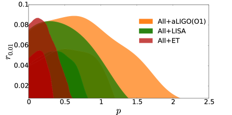
Figure 2: Marginalized posterior distributions at 68% and 95% C.L. for the parameters $r$ and $p$. “All” refers to Planck2015, HST, BAO and BK14 data.

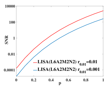
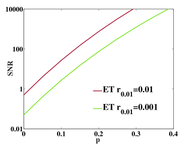
Figure 3: The SNRs of LISA configuration N2A2M2L6 and ET with respect to $p$ for different $r_{0.01}$. The duration of observation of ET is taken as 1 year.

III.2 The slow expansion with ${\cal L}_{4}$

In Galilean Genesis [58, 59] (also slow expansion scenario [60, 61]), the spacetime is flat Minkowski in infinite past and the universe is slowly expanding,

$$a\sim e^{{1\over(-t)^{n}}}\simeq 1+{1\over(-t)^{n}}$$ (12)

where $n>0$ and $H\sim{1\over(-t)^{n+1}}$ rapidly rises, after the slowly expanding phase ends, the universe reheats and the evolution of hot ‘big-bang’ starts. With the cubic Galielon, it has been found in [61] that during the slow expansion, the scale-invariant adiabatic perturbation may be produced for $n=4$, see also [62].

The original Genesis scenarios predict a blue-tilted GWs spectrum,

$$P_{T}\simeq{H^{2}_{end}\over M_{p}^{2}}\left({k\over k_{end}}\right)^{2},$$ (13)

The case is similar in ekpyrotic scenario [63](different case see[64]). Here, the pivot scale $k_{*}$ is actually $k_{*}=k_{end}$, where the subscript ‘end’ corresponds to the quantities at the ending time of the Genesis phase. Thus at CMB scale $k_{CMB}\sim 0.01\,\mathrm{Mpc}^{-1}$,

$$r_{0.01}\sim\left({k_{CMB}\over k_{end}}\right)^{2}\ll 0.001,$$ (14)

is negligibly small, see [65] for a theoretical lower limit. And at aLIGO scale, $\Omega_{\text{GW}}\sim P_{T}\sim({k_{aLIGO}\over k_{end}})^{2}$ is also far small, unless $k_{aLIGO}\simeq k_{end}$. Thus the current limit on $n_{T}$ can hardly put any constraints for the corresponding models.

In Ref.[66], based on the Horndeski theory with ${\cal L}_{4}$, it has been found that in Genesis scenario, the spectrum of primordial GWs may be flat, and even interestingly, it also may be blue-tilted with $k_{*}\sim k_{0.01}$ in Eq.(2). Recently, in [67] Nishi and Kobayashi also have found the similar case in full Horndeski theory [68]. Thus the combination of interferometers and CMB data may put the corresponding bound for it.

We first briefly review the model proposed in [66]. The Lagrangian is

$$S=\int d^{4}x\sqrt{-g}\Big{[}{1\over 2}e^{4\phi/{\cal M}}X-{1\over 8{\cal M}^{8}}X^{3}-\alpha{\cal M}^{4}\,e^{6\phi/{\cal M}}$$

$$\qquad\qquad\qquad+{M_{P}^{2}\over 2}\left(4{\cal M}^{8}/X^{2}+1\right)R-{8M_{P}^{2}{\cal M}^{8}\over X^{3}}\left[-\left(\Box\phi\right)^{2}+\nabla_{\mu}\nabla_{\nu}\phi\nabla^{\mu}\nabla^{\nu}\phi\right]\Big{]}\,,$$

where $X={\nabla_{\mu}\phi\nabla^{\mu}\phi}$. Mapping it into EFT, we have

$$f(t)=1+{4{\cal M}^{8}\over X^{2}}\,,$$ (16)

$$c(t)={1\over 2}e^{4\phi/{\cal M}}X-{3\over 8{\cal M}^{8}}X^{3}+\frac{8\mathcal{M}^{8}M_{p}^{2}}{X^{3}}\left(15H^{2}X+Y\right)\,,$$

$$\Lambda(t)=-{X^{3}\over 4{\cal M}^{8}}+\alpha{\cal M}^{4}\,e^{6\phi/{\cal M}}+\frac{8\mathcal{M}^{8}M_{p}^{2}}{X^{3}}\left(9H^{2}X+6H\dot{\phi}\ddot{\phi}-Y\right)\,,$$

$$M_{2}^{4}(t)=-{3X^{3}\over 4{\cal M}^{8}}-\frac{4\mathcal{M}^{8}M_{p}^{2}}{X^{3}}\left(90H^{2}X+Y\right)\,,$$

$$m_{3}^{3}(t)=\frac{16\mathcal{M}^{8}M_{p}^{2}}{X^{3}}\left(10HX+\dot{\phi}\ddot{\phi}\right)\,,$$

$$m_{4}^{2}(t)=\tilde{m}_{4}^{2}(t)=\frac{8\mathcal{M}^{8}M_{p}^{2}}{X^{2}}\,,$$

where $Y=11H\dot{\phi}\ddot{\phi}+2\dot{H}X-\dot{\phi}\dddot{\phi}+5\ddot{\phi}^{2}$.

We have the solution

$$e^{\phi/{\cal M}}=\left({15\over 4}\right)^{1/4}{1\over{\cal M}(t_{*}-t)},$$ (17)

$${\dot{\phi}}={{\cal M}\over(t_{*}-t)},$$ (18)

and $\alpha={2\over 3\sqrt{15}}$. Thus only one adjustable parameter ${\cal M}$ is left. The background of slow expansion is described by

$$a=a_{0}e^{\int Hdt}\simeq a_{0}(1+{1\over{\cal M}^{6}M_{P}^{2}}{1\over(t_{*}-t)^{8}})\simeq a_{0},$$ (19)

where $H\sim{1\over{\cal M}^{6}M_{P}^{2}}(t_{*}-t)^{-9}$, and the condition of slow expansion is ${\cal M}^{6}M_{P}^{2}(t_{*}-t)^{8}\gg 1$, which suggests $\epsilon\simeq-{\cal M}^{6}M_{P}^{2}(t_{*}-t)^{8}\ll-1$. Thus initially the universe is Minkowski. When ${\cal M}^{6}M_{P}^{2}(t_{*}-t)^{8}\simeq 1$, the slowly expanding phase ends. Hereafter, ${X/{\cal M}^{4}}\gg 1$, GR is recovered, and the hot big-bang universe will start.

Since $f\sim{m}_{4}^{2}/M_{p}^{2}\sim{\cal M}^{8}/X^{2}$, we have $Q_{T}\sim(t_{*}-t)^{4}$ and $c_{T}^{2}$ is constant. The GWs horizon $\sim 1/H_{T}$ is $1/H_{T}\sim{t_{*}-t}$. Thus the spectrum of primordial GWs is [66] ${P}_{T}\simeq({{\cal M}\over M_{P}})^{1/2}$. However, generally we may set $Q_{T}\sim(t_{*}-t)^{p}$, and have

$${P}_{T}\simeq\left({{\cal M}\over M_{P}}\right)^{1/2}\left({k\over k_{*}}\right)^{n_{T}},$$ (20)

where $n_{T}=4-p$, which is blue-tilted for $p<4$.

Here, the adiabatic scalar perturbation is strong blue-tilted, ${P}_{s}\simeq{{\cal M}\over M_{P}}({k\over k_{*}})^{12/5}$ and the primordial density perturbation responsible for the observations may be induced by the perturbation of a light scalar field, see [69] for a review, which is insensitive to $Q_{T}$.

In Fig.4, we see that the combination of Planck2015+BK14 and aLIGO O1 data gives

$$3.4\lesssim p={d\ln{Q_{T}}\over d\ln{H_{T}}}\lesssim 4.6$$ (21)

at 68% C.L. for $r_{0.01}\lesssim 0.01$. Thus we could have $r_{0.01}\simeq 0.01-0.001$ at CMB scale, which is detectable for the ongoing CMB B-mode polarization experiments. Here, since $Q_{T}\sim f\sim m_{4}$, we have $p={d\ln{f}\over d\ln{H_{T}}}={d\ln{m_{4}}\over d\ln{H_{T}}}$. In the future, LISA and ET will put stronger bounds, which are $3.6\lesssim p\lesssim 4.6$ and $3.7\lesssim p\lesssim 4.6$, respectively.

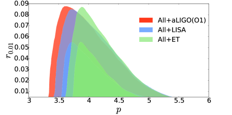
Figure 4: Marginalized posterior distributions at 68% and 95% C.L. for the parameters $r$ and $p$. “All” refers to Planck2015, HST, BAO and BK14 data.

IV Conclusion

The spectrum of primordial GWs, especially $n_{T}$, carries significant information about the primordial universe. Though the primordial GWs remains undetected, combining data at different frequency-bands is able to put tighter constraint on $n_{T}$ than the CMB alone, which helps to deepen our understanding for the origin of the universe.

We perform a combination of Planck2015+BK14 data and the upper limit put by recent aLIGO on stochastic GWs background, as well as the expected ET and space-based LISA sensetivities. Assuming the spectrum of primordial GWs is described by (2) with $k_{*}=0.01\,\mathrm{Mpc}^{-1}$, we find that with recent CMB+aLIGO O1 dataset, the current limit is $r_{0.01}<0.066$ and $n_{T}=0.016^{+0.614}_{-0.989}$ at 95% C.L., and also for forecasts, we find that $r_{0.01}<0.062$ and $n_{T}=-0.050^{+0.612}_{-0.992}$ for the CMB+LISA set, and $r_{0.01}<0.061$, $n_{T}=-0.184^{+0.534}_{-0.877}$ for the CMB+ET set. Thus at present the CMB+aLIGO O1 dataset has significantly improved the limit on $n_{T}$, and it is expected that in the future LISA and ET would make limits tighter.

We also explore how to confront the models of early universe scenarios, which produce blue-tilted GWs spectrum, with the corresponding data. We apply the combined analysis of interferometers and CMB data to some early universe models, which may be mapped into EFT. In particular, for the inflation model with diminishing $c_{T}$, we find that the current limit is ${{\dot{m}}_{4}/(H_{inf}m_{4})}\lesssim 1.2$ at 68% C.L. for $r_{0.01}\lesssim 0.01$ and $0<c_{T}^{2}\ll 1$. In the future, LISA and ET could put stronger limits on $m_{4}$, which are ${{\dot{m}}_{4}/(H_{inf}m_{4})}\lesssim 0.8$ and $0.3$, respectively.

Acknowledgments

We thank Sai Wang for his help in program and Bin Hu for his valuable comments on the earlier manuscript. We acknowledge the use of CAMB and CosmoMC. This work is supported by NSFC, No. 11222546, 11575188, 11690021, and also supported by the Strategic Priority Research Program of CAS, No. XDA04075000, XDB23010100. Z.G.Liu is supported in part by the fifty-seventh batch of China Postdoctoral Fund.

Appendix A EFT and tensor perturbation

With the ADM line element, we have

$$g_{\mu\nu}=\left(\begin{array}[]{cc}N_{k}N^{k}-N^{2}&N_{j}\\ N_{i}&h_{ij}\\ \end{array}\right)\,,\qquad g^{\mu\nu}=\left(\begin{array}[]{cc}-N^{-2}&{N^{j}\over N^{2}}\\ {N^{i}\over N^{2}}&h^{ij}-{N^{i}N^{j}\over N^{2}}\\ \end{array}\right)\,,\qquad$$ (22)

and $\sqrt{-g}=N\sqrt{h}$, where $N_{i}=h_{ij}N^{j}$. We can define the unit one-form tangent vector $n_{\nu}=n_{0}(dt/dx^{\mu})=(-N,0,0,0)$ and $n^{\nu}=g^{\mu\nu}n_{\mu}=({1/N},-{N^{i}/N})$, which satisfies $n_{\mu}n^{\mu}=-1$. The induced 3-dimensional metric on the hypersurface is $H_{\mu\nu}=g_{\mu\nu}+n_{\mu}n_{\nu}$, thus

$$H_{\mu\nu}=\left(\begin{array}[]{cc}N_{k}N^{k}&N_{j}\\ N_{i}&h_{ij}\\ \end{array}\right)\,,\qquad H^{\mu\nu}=\left(\begin{array}[]{cc}0&0\\ 0&h^{ij}\\ \end{array}\right)\,.\qquad$$ (23)

The Ricci scalar is decomposed as

$$R=R^{(3)}-K^{2}+K_{\mu\nu}K^{\mu\nu}+2\nabla_{\mu}(Kn^{\mu}-n^{\nu}\nabla_{\nu}n^{\mu})~{}.$$ (24)

where $R^{(3)}$ is the induced 3-dimensional Ricci scalar associated with $H_{\mu\nu}$, and the extrinsic curvature $K_{\mu\nu}$ on the hypersurface is $K_{\mu\nu}\equiv{1\over 2}{\cal L}_{n}H_{\mu\nu}$ and ${\cal L}_{n}$ is the Lie derivative with respective to $n^{\mu}$.

Without higher-order spatial derivatives, the EFT of cosmological perturbation reads [24, 25]

$$S = \int d^{4}x\sqrt{-g}\Big{[}{M_{p}^{2}\over 2}f(t)R-\Lambda(t)-c(t)g^{00}$$ (25)

$$+{M_{2}^{4}(t)\over 2}(\delta g^{00})^{2}-{m_{3}^{3}(t)\over 2}\delta K\delta g^{00}-m_{4}^{2}(t)\left(\delta K^{2}-\delta K_{\mu\nu}\delta K^{\mu\nu}\right)$$

$$+{\tilde{m}_{4}^{2}(t)\over 2}R^{(3)}\delta g^{00}\Big{]}+S_{m}[g_{\mu\nu},\psi_{m}]\,,$$

where $\delta g^{00}=g^{00}+1$, $\delta K_{\mu\nu}=K_{\mu\nu}-H_{\mu\nu}H$, $\delta K^{\mu\nu}=K^{\mu\nu}-H^{\mu\nu}H$, and $\delta K=\delta K^{\mu}_{\mu}=K^{\mu}_{\mu}-3H$. The coefficients $(f,c,\Lambda,M_{2},m_{3}$, $m_{4},{\tilde{m}}_{4})$ specify the corresponding theories. A particular subset $(m_{4}={\tilde{m}}_{4})$ of EFT (25) is the Horndeski theory [26]. $S_{m}[g_{\mu\nu},\psi_{m}]$ is the matter part, which is minimally coupled to the metric $g_{\mu\nu}$.

In the unitary gauge, we set

$$h_{ij}=a^{2}e^{2\zeta}(e^{\gamma})_{ij},\qquad\gamma_{ii}=0=\partial_{i}\gamma_{ij}\,.$$ (26)

References

- [1] A. A. Starobinsky, JETP Lett. 30, 682 (1979) [Pisma Zh. Eksp. Teor. Fiz. 30, 719 (1979)].
- [2] V. A. Rubakov, M. V. Sazhin and A. V. Veryaskin, Phys. Lett. B115, 189 (1982).
- [3] M. Maggiore, Phys. Rept. 331, 283 (2000) [gr-qc/9909001].
- [4] M. Guzzetti, C., N. Bartolo, Liguori, M. and S. Matarrese, Riv. Nuovo Cim. 39 (2016) 9, 399 [arXiv:1605.01615 [astro-ph.CO]].
- [5] N. Bartolo et al., arXiv:1610.06481 [astro-ph.CO].
- [6] A. D. Linde, Phys. Lett. B 108, 389 (1982).
- [7] A. Albrecht and P. J. Steinhardt, Phys. Rev. Lett. 48, 1220 (1982).
- [8] Y. Cai, Y. T. Wang and Y. S. Piao, Phys. Rev. D 94, 4, 043002 (2016) [arXiv:1602.05431 [astro-ph.CO]].
- [9] Y. Cai, Y. T. Wang and Y. S. Piao, Phys. Rev. D 93, 6, 063005 (2016) [arXiv:1510.08716 [astro-ph.CO]].
- [10] M. Kamionkowski, A. Kosowsky and A. Stebbins, Phys. Rev. Lett. 78, 2058 (1997) doi:10.1103/PhysRevLett.78.2058 [astro-ph/9609132].
- [11] M. Kamionkowski, A. Kosowsky and A. Stebbins, Phys. Rev. D 55, 7368 (1997) doi:10.1103/PhysRevD.55.7368 [astro-ph/9611125].
- [12] P. A. R. Ade et al. [BICEP2 and Planck Collaborations], Phys. Rev. Lett. 114, 101301 (2015) [arXiv:1502.00612 [astro-ph.CO]].
- [13] P. A. R. Ade et al. [BICEP2 and Keck Array Collaborations], Phys. Rev. Lett. 116, 031302 (2016) [arXiv:1510.09217 [astro-ph.CO]].
- [14] W. Zhao and D. Baskaran, Phys. Rev. D 79, 083003 (2009) doi:10.1103/PhysRevD.79.083003 [arXiv:0902.1851 [astro-ph.CO]].
- [15] Q. G. Huang, S. Wang and W. Zhao, JCAP 1510, no. 10, 035 (2015) doi:10.1088/1475-7516/2015/10/035 [arXiv:1509.02676 [astro-ph.CO]].
- [16] B. P. Abbott et al. [LIGO Scientific and Virgo Collaborations], Phys. Rev. Lett. 116, 6, 061102 (2016) [arXiv:1602.03837 [gr-qc]].
- [17] B. P. Abbott et al. [LIGO Scientific and Virgo Collaborations], Phys. Rev. Lett. 116, 13, 131102 (2016) [arXiv:1602.03847 [gr-qc]].
- [18] B. P. Abbott et al. [The LIGO Scientific and the Virgo Collaborations], arXiv:1612.02029 [gr-qc].
- [19] Z. G. Liu, H. Li and Y. S. Piao, Phys. Rev. D 90, 8, 083521 (2014) [arXiv:1405.1188 [astro-ph.CO]].
- [20] H. G. Li, Y. Cai and Y. S. Piao, arXiv:1605.09586 [gr-qc].
- [21] C. Cheung, P. Creminelli, A. L. Fitzpatrick, J. Kaplan and L. Senatore, JHEP 0803, 014 (2008) [arXiv:0709.0293 [hep-th]].
- [22] S. Weinberg, Phys. Rev. D 77, 123541 (2008) [arXiv:0804.4291 [hep-th]].
- [23] G. Gubitosi, F. Piazza and F. Vernizzi, JCAP 1302, 032 (2013) [arXiv:1210.0201 [hep-th]].
- [24] J. Gleyzes, D. Langlois, F. Piazza and F. Vernizzi, JCAP 1308, 025 (2013) [arXiv:1304.4840 [hep-th]].
- [25] F. Piazza and F. Vernizzi, Class. Quant. Grav. 30, 214007 (2013) [arXiv:1307.4350 [hep-th]].
- [26] G. W. Horndeski, Int. J. Theor. Phys. 10, 363 (1974).
- [27] J. Gleyzes, D. Langlois, F. Piazza and F. Vernizzi, Phys. Rev. Lett. 114, 21, 211101 (2015) [arXiv:1404.6495 [hep-th]].
- [28] Y. Cai, Y. Wan, H. G. Li, T. Qiu and Y. S. Piao, arXiv:1610.03400 [gr-qc].
- [29] P. Creminelli, D. Pirtskhalava, L. Santoni and E. Trincherini, JCAP 1611, 11, 047 (2016) [arXiv:1610.04207 [hep-th]].
- [30] P. D. Meerburg, R. Hlozek, B. Hadzhiyska and J. Meyers, Phys. Rev. D 91, 10, 103505 (2015) [arXiv:1502.00302 [astro-ph.CO]].
- [31] G. Cabass, L. Pagano, L. Salvati, M. Gerbino, E. Giusarma and A. Melchiorri, Phys. Rev. D 93, 6, 063508 (2016) [arXiv:1511.05146 [astro-ph.CO]].
- [32] P. D. Lasky et al., Phys. Rev. X 6, 1, 011035 (2016) [arXiv:1511.05994 [astro-ph.CO]].
- [33] T. L. Smith, M. Kamionkowski and A. Cooray, Phys. Rev. D 73, 023504 (2006) doi:10.1103/PhysRevD.73.023504 [astro-ph/0506422].
- [34] T. L. Smith, M. Kamionkowski and A. Cooray, Phys. Rev. D 78, 083525 (2008) doi:10.1103/PhysRevD.78.083525 [arXiv:0802.1530 [astro-ph]].
- [35] P. A. Seoane et al. [eLISA Collaboration], arXiv:1305.5720 [astro-ph.CO].
- [36] A. Ricciardone, arXiv:1612.06799 [astro-ph.CO].
- [37] S. Hild et al., Class. Quant. Grav. 28, 094013 (2011) [arXiv:1012.0908 [gr-qc]].
- [38] M. S. Turner, M. J. White and J. E. Lidsey, Phys. Rev. D 48, 4613 (1993) [astro-ph/9306029].
- [39] W. Zhao and Y. Zhang, Phys. Rev. D 74, 043503 (2006) doi:10.1103/PhysRevD.74.043503 [astro-ph/0604458].
- [40] W. Zhao, Phys. Rev. D 83, 104021 (2011) doi:10.1103/PhysRevD.83.104021 [arXiv:1103.3927 [astro-ph.CO]].
- [41] W. Zhao, Y. Zhang, X. P. You and Z. H. Zhu, Phys. Rev. D 87, no. 12, 124012 (2013) doi:10.1103/PhysRevD.87.124012 [arXiv:1303.6718 [astro-ph.CO]].
- [42] S. Kuroyanagi, T. Takahashi and S. Yokoyama, JCAP 1502, 003 (2015) [arXiv:1407.4785 [astro-ph.CO]].
- [43] R. Adam et al. [Planck Collaboration], arXiv:1502.01582 [astro-ph.CO].
- [44] N. Scoville et al., Astrophys. J. Suppl. 172, 38 (2007) [astro-ph/0612306].
- [45] F. Beutler et al., Mon. Not. Roy. Astron. Soc. 416, 3017 (2011) [arXiv:1106.3366 [astro-ph.CO]].
- [46] A. J. Ross, L. Samushia, C. Howlett, W. J. Percival, A. Burden and M. Manera, Mon. Not. Roy. Astron. Soc. 449, 1, 835 (2015) [arXiv:1409.3242 [astro-ph.CO]].
- [47] L. Anderson et al. [BOSS Collaboration], Mon. Not. Roy. Astron. Soc. 441, 1, 24 (2014) [arXiv:1312.4877 [astro-ph.CO]].
- [48] A. Lewis and S. Bridle, Phys. Rev. D 66, 103511 (2002) [astro-ph/0205436].
- [49] A. Lewis, A. Challinor and A. Lasenby, Astrophys. J. 538, 473 (2000) [astro-ph/9911177].
- [50] Q. G. Huang and S. Wang, JCAP 1506, 06, 021 (2015) [arXiv:1502.02541 [astro-ph.CO]].
- [51] A. Klein et al., Phys. Rev. D 93, 2, 024003 (2016) [arXiv:1511.05581 [gr-qc]].
- [52] T. L. Smith and R. Caldwell, arXiv:1609.05901 [gr-qc].
- [53] X. J. Liu, W. Zhao, Y. Zhang and Z. H. Zhu, Phys. Rev. D 93, no. 2, 024031 (2016) doi:10.1103/PhysRevD.93.024031 [arXiv:1509.03524 [astro-ph.CO]].
- [54] Y. S. Piao and Y. Z. Zhang, Phys. Rev. D 70, 063513 (2004) [astro-ph/0401231].
- [55] Y. S. Piao, Phys. Rev. D 78, 023518 (2008) [arXiv:0712.3328 [gr-qc]]; Z. G. Liu, Z. K. Guo and Y. S. Piao, Eur. Phys. J. C 74, 8, 3006 (2014) [arXiv:1311.1599 [astro-ph.CO]].
- [56] D. Cannone, G. Tasinato and D. Wands, JCAP 1501, 01, 029 (2015) [arXiv:1409.6568 [astro-ph.CO]].
- [57] N. Bartolo, D. Cannone, A. Ricciardone and G. Tasinato, JCAP 1603, 03, 044 (2016) [arXiv:1511.07414 [astro-ph.CO]].
- [58] P. Creminelli, A. Nicolis and E. Trincherini, JCAP 1011, 021 (2010) [arXiv:1007.0027 [hep-th]].
- [59] P. Creminelli, K. Hinterbichler, J. Khoury, A. Nicolis and E. Trincherini, JHEP 1302, 006 (2013) [arXiv:1209.3768 [hep-th]].
- [60] Y. S. Piao and E. Zhou, Phys. Rev. D 68, 083515 (2003) [hep-th/0308080].
- [61] Z. G. Liu, J. Zhang and Y. S. Piao, Phys. Rev. D 84, 063508 (2011) [arXiv:1105.5713]; Z. G. Liu and Y. S. Piao, Phys. Lett. B 718, 734 (2013) [arXiv:1207.2568 [gr-qc]].
- [62] S. Nishi and T. Kobayashi, JCAP 1503, 03, 057 (2015) [arXiv:1501.02553 [hep-th]].
- [63] L. A. Boyle, P. J. Steinhardt and N. Turok, Phys. Rev. D 69, 127302 (2004) [hep-th/0307170].
- [64] I. Ben-Dayan, JCAP 1609, no. 09, 017 (2016) doi:10.1088/1475-7516/2016/09/017 [arXiv:1604.07899 [astro-ph.CO]].
- [65] D. Baumann, P. J. Steinhardt, K. Takahashi and K. Ichiki, Phys. Rev. D 76, 084019 (2007) [hep-th/0703290].
- [66] Y. Cai and Y. S. Piao, JHEP 1603, 134 (2016) [arXiv:1601.07031 [hep-th]].
- [67] S. Nishi and T. Kobayashi, arXiv:1611.01906 [hep-th].
- [68] T. Kobayashi, M. Yamaguchi and J. Yokoyama, Prog. Theor. Phys. 126, 511 (2011) [arXiv:1105.5723 [hep-th]].
- [69] V. A. Rubakov, Phys. Usp. 57, 128 (2014) [arXiv:1401.4024 [hep-th]].