A Fully Convolutional Deep Auditory Model for Musical Chord Recognition

Abstract

Chord recognition systems depend on robust feature extraction pipelines. While these pipelines are traditionally hand-crafted, recent advances in end-to-end machine learning have begun to inspire researchers to explore data-driven methods for such tasks. In this paper, we present a chord recognition system that uses a fully convolutional deep auditory model for feature extraction. The extracted features are processed by a Conditional Random Field that decodes the final chord sequence. Both processing stages are trained automatically and do not require expert knowledge for optimising parameters. We show that the learned auditory system extracts musically interpretable features, and that the proposed chord recognition system achieves results on par or better than state-of-the-art algorithms.

Index Terms—  chord recognition, convolutional neural networks, conditional random fields

1 Introduction

Chord Recognition is a long-standing topic of interest in the music information research (MIR) community. It is concerned with recognising (and transcribing) chords in audio recordings of music, a labor-intensive task that requires extensive musical training if done manually. Chords are a highly descriptive feature of music and useful e.g. for creating lead sheets for musicians or as part of higher-level tasks such as cover song identification.

A chord can be defined as multiple notes perceived simultaneously in harmony. This does not require the notes to be played simultaneously—a melody or a chord arpeggiation can imply the perception of a chord, even if intertwined with out-of-chord notes. Through this perceptual process, the identification of a chord is sometimes subject to interpretation even among trained experts. This inherent subjectivity is evidenced by diverse ground-truth annotations for the same songs and discussions about proper evaluation metrics [1].

Typical chord recognition pipelines comprise three stages: feature extraction, pattern matching, and chord sequence decoding. Feature extraction transforms audio signals into representations which emphasise content related to harmony. Pattern matching assigns chord labels to such representations but works on single frames or local context only. Chord sequence decoding puts the local detection into global context by predicting a chord sequence for the complete audio.

Originally hand-crafted [2], all three stages have seen attempts to be replaced by data-driven methods. For feature extraction, linear regression [3], feed-forward neural networks [4] and convolutional neural networks [5] were explored; these approaches fit a transformation from a general time-frequency representation to a manually defined one that is specifically useful for chord recognition, like chroma vectors or a “Tonnetz” representation. Pattern matching often uses Gaussian mixture models [6], but has seen work on chord classification directly from a time-frequency representation using convolutional neural networks [7]. For sequence decoding, hidden Markov models [8], conditional random fields [9] and recurrent neural networks [10] are natural choices; however, the vast majority of chord recognition systems still rely on hidden Markov models (HMMs): only one approach used conditional random fields (CRFs) in combination with simple chroma features for this task [9], with limited success. This warrants further exploration of this model class, since it has proven to out-perform HMMs in other domains.

In this paper, we present a novel end-to-end chord recognition system that combines a fully convolutional neural network (CNN) for feature extraction with a CRF for chord sequence decoding. Fully convolutional neural networks replace the stack of dense layers traditionally used in CNNs for classification with global average pooling (GAP) [11], which reduces the number of trainable parameters and improves generalisation. Similarly to [7], we train the CNN to directly predict chord labels for each audio frame, but instead of using these predictions directly, we use the hidden representation computed by the CNN as features for the subsequent pattern matching and chord sequence decoding stage. We call the feature-extracting part of the CNN auditory model.

For pattern matching and chord sequence decoding, we connect a CRF to the auditory model. Combining neural networks with CRFs gives a fully differentiable model that can be learned jointly, as shown in [12, 13]. For the task at hand, however, we found it advantageous to train both parts separately, both in terms of convergence time and performance.

2 Feature Extraction

Feature extraction is a two-phase process. First, we convert the signal into a time-frequency representation in the pre-processing stage. Then, we feed this representation to a CNN and train it to classify chords. We take the activations of a hidden layer in the network as high-level feature representation, which we then use to decode the final chord sequence.

2.1 Pre-processing

The first stage of our feature extraction pipeline transforms the input audio into a time-frequency representation suitable as input to a CNN. As described in Sec. 2.2, CNNs consist of fixed-size filters that capture local structure, which requires the spatial relations to be similarly distributed in each area of the input. To achieve this, we compute the magnitude spectrogram of the audio and apply a filterbank with logarithmically spaced triangular filters. This gives us a time-frequency representation in which distances between notes (and their harmonics) are equal in all areas of the input. Finally, we logarithmise the filtered magnitudes to compress the value range. Mathematically, the resulting time-frequency representation L of an audio recording is defined as

$$\mathbf{L}=\log\left(1+\mathbf{B}^{\triangle}_{\text{Log}}\left\lvert\mathbf{S}\right\rvert\right),$$

where $\mathbf{S}$ is the short-time Fourier transform (STFT) of the audio, and $\mathbf{B}^{\triangle}_{\text{Log}}$ is the logarithmically spaced triangular filterbank. To be concise, we will refer to $\mathbf{L}$ as spectrogram in the remainder of this paper.

We feed the network spectrogram frames with context, i.e. the input to the network is not a single column $\mathbf{l}_{i}$ of $\mathbf{L}$, but a matrix $\mathbf{X}_{i}=\left[\mathbf{l}_{i-C},\ldots,\mathbf{l}_{i},\ldots,\mathbf{l}_{i+C}\right]$, where $i$ is the index of the target frame, and $C$ is the context size.

We chose the parameter values based on our previous study on data-driven feature extraction for chord recognition [4] and a number of preliminary experiments. We use a frame size of 8192 with a hop size of 4410 at a sample rate of 44100 Hz for the STFT. The filterbank comprises 24 filters per octave between 65 Hz and 2100 Hz. The context size $C=7$, thus each $\mathbf{X}_{i}$ represents 1.5 sec. of audio. Our choice of parameters results in an input dimensionality of $\mathbf{X}_{i}\in\mathbb{R}^{105\times 15}$.

2.2 Auditory Model

To extract discriminative features from the input, in [4], we used a simple deep neural network (DNN) to compute chromagrams, concise descriptors of harmonic content. From these chromagrams, we used a simple classifier to predict chords in a frame-wise manner. Despite the network being simple conceptually, due to the dense connections between layers, the model had 1.9 million parameters.

In this paper, we use a CNN for feature extraction. CNNs differ from traditional deep neural networks by including two additional types of computational layers: convolutional layers compute a 2-dimensional convolution of their input with a set of fixed-sized, trainable kernels per feature map, followed by a (usually non-linear) activation function; pooling layers sub-sample the input by aggregating over a local neighbourhood (e.g. the maximum of a $2\times 2$ patch). The former can be re-formulated as a dense layer using a sparse weight matrix with tied weights. This interpretation indicates the advantages of convolutional layers: fewer parameters and better generalisation.

CNNs typically consist of convolutional lower layers that act as feature extractors, followed by fully connected layers for classification. Such layers are prone to over-fitting and come with a large number of parameters. We thus follow [11] and use global average pooling (GAP) to replace them. To further prevent over-fitting, we apply dropout [14], and use batch normalisation [15] to speed up training convergence.

Table 1 details our model architecture, which consists of 900k parameters, roughly 50% of the original DNN. Inspired by the architecture presented in [16], We opted for multiple lower convolutional layers with small $3\times 3$ kernels, followed by a layer computing 128 feature maps using $12\times 9$ kernels. The intuition is that these bigger kernels can aggregate harmonic information for the classification part of the network. We will denote the output of this layer as ${\mathbf{F}}_{i}$, the features extracted from input ${\mathbf{X}}_{i}$.

Layer Type	Parameters	Padding	Output Size
Input			$105\times 15$
Conv-Rectify	$32\times 3\times 3$	yes	$32\times 105\times 15$
Conv-Rectify	$32\times 3\times 3$	yes	$32\times 105\times 15$
Conv-Rectify	$32\times 3\times 3$	yes	$32\times 105\times 15$
Conv-Rectify	$32\times 3\times 3$	yes	$32\times 105\times 15$
Pool-Max	$2\times 1$		$32\times 52\times 15$
Conv-Rectify	$64\times 3\times 3$	no	$64\times 50\times 13$
Conv-Rectify	$64\times 3\times 3$	no	$64\times 48\times 11$
Pool-Max	$2\times 1$		$64\times 24\times 11$
Conv-Rectify	$128\times 12\times 9$	no	$128\times 13\times 3$
Conv-Linear	$25\times 1\times 1$	no	$25\times 13\times 3$
Pool-Avg	$13\times 3$		$25\times 1\times 1$
Softmax			$25$

Table 1: Proposed CNN architecture. Batch normalisation is performed after each convolution layer. Dropout with probability 0.5 is applied at horizontal rules in the table. All convolution layers use rectifier units [17], except the last, which is linear. The bottom three layers represent the GAP, replacing fully connected layers for classification.

We target a reduced chord alphabet in this work (major and minor chords for 12 semitones) resulting in 24 classes plus a “no chord” class. This is a common restriction used in the literature on chord recognition [18]. The GAP construct thus learns a weighted average of the 128 feature maps for each of the 25 classes using the $1\times 1$ convolution and average pooling layer. Applying the softmax function then ensures that the output sums to 1 and can be interpreted as a probability distribution of class labels given the input.

Following [19], the activations of the network’s hidden layers can be interpreted as hierarchical feature representations of the input data. We will thus use ${\mathbf{F}}_{i}$ as a feature representation for the subsequent parts of our chord recognition pipeline.

2.3 Training and Data Augmentation

We train the auditory model in a supervised manner using the Adam optimisation method [20] with standard parameters, minimising the categorical cross-entropy between true targets ${\mathbf{y}}_{i}$ and network output $\tilde{{\mathbf{y}}}_{i}$. Including a regularisation term, the loss is defined as

$${\cal L}=-\frac{1}{D}\sum_{i=1}^{D}{\mathbf{y}}_{i}\log(\tilde{{\mathbf{y}}}_{i})+\lambda\left|\mathbf{\theta}\right|_{2},$$

where $D$ is the number of frames in the training data, $\lambda=10^{-7}$ the $l_{2}$ regularisation factor, and $\theta$ the network parameters. We process the training set in mini-batches of size 512, and stop training if the validation accuracy does not improve for 5 epochs.

We apply two types of data manipulations to increase the variety of training data and prevent model over-fitting. Both exploit the fact that the frequency axis of our input representation is linear in pitch, and thus facilitates the emulation of pitch-shifting operations. The first operation, as explored in [7], shifts the spectrogram up or down in discrete semitone steps by a maximum of 4 semitones. This manipulation does not preserve the label, which we thus adjust accordingly. The second operation emulates a slight detuning by shifting the spectrogram by fractions of up to 0.4 of a semitone. Here, the label remains unchanged. We process each data point in a mini-batch with randomly selected shift distances. The network thus almost never sees exactly the same input during training. We found these data augmenting operations to be crucial to prevent over-fitting.

3 Chord Sequence Decoding

Using the predictions of the pattern matching stage directly (in our case, the predictions of the CNN) often gives good results in terms of frame-wise accuracy. However, chord sequences obtained this way are often fragmented. The main purpose of chord sequence decoding is thus to smooth the reported sequence. Here, we use a linear-chain CRF [21] to introduce inter-frame dependencies and find the optimal state sequence using Viterbi decoding.

3.1 Conditional Random Fields

Conditional random fields are probabilistic energy-based models for structured classification. They model the conditional probability distribution

$$p\left({\mathbf{Y}}\mid{\mathbf{X}}\right)=\frac{\exp\left[E\left({\mathbf{Y}},{\mathbf{X}}\right)\right]}{\sum_{{\mathbf{Y}}^{\prime}}\exp\left[E\left({\mathbf{Y}}^{\prime},{\mathbf{X}}\right)\right]}$$ (1)

where ${\mathbf{Y}}$ is the label vector sequence $\left[{\mathbf{y}}_{0},\ldots,{\mathbf{y}}_{N}\right]$, and ${\mathbf{X}}$ the feature vector sequence of same length. We assume each ${\mathbf{y}}_{i}$ to be the target label in one-hot encoding. The energy function is defined as

$$\begin{split}E\left({\mathbf{Y}},{\mathbf{X}}\right)&=\sum_{i=1}^{N}\left[{\mathbf{y}}_{n-1}^{\top}{\mathbf{A}}{\mathbf{y}}_{n}+{\mathbf{y}}_{n}^{\top}{\mathbf{c}}+{\mathbf{x}}_{n}^{\top}{\mathbf{W}}{\mathbf{y}}_{n}\right]\\ &\quad+{\mathbf{y}}_{0}^{\top}\pi+{\mathbf{y}}_{N}^{\top}\tau\end{split}$$ (2)

where ${\mathbf{A}}$ models the inter-frame potentials, ${\mathbf{W}}$ the frame-input potentials, ${\mathbf{c}}$ the label bias, $\pi$ the potential of the first label, and $\tau$ the potential of the last label. This form of energy function defines a linear-chain CRF.

From Eq. 1 and 2 follows that a CRF can be seen as generalised logistic regression. They become equivalent if we set ${\mathbf{A}}$, $\pi$ and $\tau$ to 0. Further, logistic regression is equivalent to a softmax output layer of a neural network. We thus argue that a CRF whose input is computed by a neural network can be interpreted as a generalised softmax output layer that allows for dependencies between individual predictions. This makes CRFs a natural choice for incorporating dependencies between predictions of neural networks.

3.2 Model Definition and Training

Our model has 25 states ($\text{12 semitones}\times\{\text{major},\text{minor}\}$ and a “no-chord” class). These states are connected to observed features through the weight matrix ${\mathbf{W}}$, which computes a weighted sum of the features for each class. This corresponds to what the global-average-pooling part of the CNN does. We will thus use the input to the GAP-part, ${\mathbf{F}}_{i}$, averaged for each of the 128 feature maps, as input to the CRF. We can pull the averaging operation from the last layer to right after the feature-extraction layer, because the operations in between (linear convolution, batch normalisation) are linear and no dropout is performed at test-time.

Formally, we will denote the input sequence as $\overline{{\mathbf{F}}}\in\mathbb{R}^{128\times N}$, where each column $\overline{{\mathbf{f}}}_{i}$ is the averaged feature output of the CNN for a given input ${\mathbf{X}}_{i}$. Our CRF thus models $p\left({\mathbf{Y}}\mid\overline{{\mathbf{F}}}\right)$.

As with the CNN, we train the CRF using Adam, but set a higher learning rate of 0.01. The mini-batches consist of 32 sequences with a length of 1024 frames (102.3 sec) each. As optimisation criterion, we use the $l_{1}$-regularized negative log-likelihood of all sequences in the data set:

$${\cal L}=-\frac{1}{S}\sum_{i=1}^{S}\log p\left({\mathbf{Y}}_{i}\mid\overline{{\mathbf{F}}}_{i}\right)+\lambda\left|\xi\right|_{1},$$

where $S$ is the number of sequences in the data set, $\lambda=10^{-4}$ is the $l_{1}$ regularization factor, and $\xi$ are the CRF parameters. We stop training when validation accuracy does not increase for 5 epochs.

4 Experiments

	Isophonics	Robbie Williams	RWC
CB3	82.2	-	-
KO1	82.7	-	-
NMSD2	82.0	-	-
Proposed	82.9	82.8	82.5

Table 2: Weighted Chord Symbol Recall of major and minor chords achieved by different algorithms. The results of NMSD2 are statistically significantly worse than others, according to a Wilcoxon signed-rank test. Note that train and test data overlaps for CB3, KO1 and NMSD2, while the results of our method are determined by 8-fold cross-validation.

We evaluate the proposed system using 8-fold cross-validation on a compound dataset that comprises the following subsets: Isophonics: 180 songs by The Beatles, 19 songs by Queen, and 18 songs by Zweieck, totalling 10:21 hours of audio. RWC Popular [22]: 100 songs in the style of American and Japanese pop music originally recorded for this data set, totalling 6:46 hours of audio. Robbie Williams [23]: 65 songs by Robbie Williams, totalling 4:30 hours of audio.

As evaluation measure, we compute the Weighted Chord Symbol Recall (WCSR), often called Weighted Average Overlap Ratio (WAOR), of major and minor chords as implemented in the “mir_eval” library [24]: $\mathcal{R}=\nicefrac{{t_{c}}}{{t_{a}}}$, where $t_{c}$ is the total time where the prediction corresponds to the annotation, and $t_{a}$ is the total duration of annotations of the respective chord classes (major and minor chords, in our case).

We compare our results to the three best-performing algorithms in the MIREX competition in 2013 (no superior algorithm has been submitted to MIREX since then): CB3, based on [6]; KO1, [25]; and NMSD2, [26].

4.1 Results

The results presented for the reference algorithms differ from those found on the MIREX website. This is because of minor differences in the implementation of the evaluation libraries. To ensure a fairer comparison, we obtained the predictions of the compared algorithms and ran the same evaluation code for all approaches. Note however, that for the reference algorithms there is a known overlap between train and test set, and the obtained results might be optimistic.

Table 2 shows the results of our method compared to three state-of-the-art algorithms. We can see that the proposed method performs slightly better (but not statistically significant), although the train set of the reference methods overlaps with the test set.

5 Auditory Model Analysis

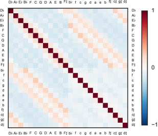
Fig. 1: Correlation between weight vectors of chord classes. Rows and columns represent chords. Major chords are represented by upper-case letters, minor chords by lower-case letters. The order of chords within a chord quality is determined by the circle of fifths. We observe that weight vectors of chords close in the circle of fifths (such as ‘C’, ‘F’, and ‘G’) correlate positively. Same applies to chords that share notes (such as ‘C’ and ‘a’, or ‘C’ and ‘c’).

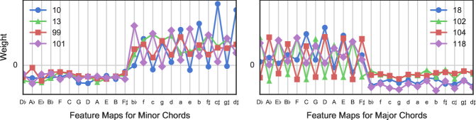
Fig. 2: Connection weights of selected feature maps to chord classes. Chord classes are ordered according to the circle of fifths, such that harmonically close chords are close to each other. In the left plot, we selected feature maps that have a high average contribution to minor chords. In the right plot, those with high contribution to major chords. Feature maps with high average weights to minor chords show negative connections to all major chords. Within minor chords, we observe that two of them (10 and 101) discriminate between chords that are harmonically close (zig-zag pattern). We observe a similar pattern in the right plot.

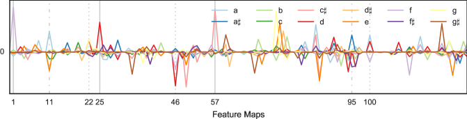
Fig. 3: Contribution of feature maps to pitch classes. Although these results are noisy, we observe that some feature maps seem to specialise on detecting the presence (or absence) pitch classes. For example, feature maps 1, 25, and 57 detect single pitch classes; feature maps 22, 46, and 100 contribute to pairs of related pitch classes—perfect fifth between ‘g’ and ‘d’ in the 22^nd, minor third between ‘d’ and ‘f’ in the 46^th, and major third between ‘a’ and ‘c$\sharp$’ in the 85^th feature map. Note that the 100^th feature map also slightly discriminates ‘d’ and ‘a’ from ‘f’, which would form a d-minor triad together. Other feature maps that discriminate between pitch classes include the 11^th (‘a’ vs. ‘e’, perfect fifth) and the 95^th (‘f$\sharp$’ vs.‘a$\sharp$’, major third).

Following [11], the final feature maps of a GAP network can be interpreted as “category confidence maps”. Such confidence maps will have a high average value if the network is confident that the input is of the respective category. In our architecture, the average activation of a confidence map can be expressed as a weighted average over the (batch-normalised) feature maps of the preceding layer. We thus have 128 weights for each of the 25 categories (chord classes).

We wanted to see whether the penultimate feature maps ${\mathbf{F}}_{i}$ can be interpreted in a musically meaningful way. To this end, we first analysed the similarity of the weight vectors for each chord class by computing their correlation. The result is shown in Fig. 1. We see a systematic correlation between weight vectors of chords that share notes or are close to each other in the circle of fifths. The patterns within minor chords are less clear. This might be because minor chords are under-represented in the data, and the network could not learn systematic patterns from this limited amount.

Furthermore, we wanted to see if the network learned to distinguish major and minor modes independently of the root note. To this end, we selected the four feature maps with the highest connection weights to major and minor chords respectively and plotted their contribution to each chord class in Fig. 2. Here, an interesting pattern emerges: feature maps with high average weights to minor chords have negative connections to all major chords. High activations in these feature maps thus make all major chords less likely. However, they tend to be specific on which minor chords they favour. We observe a zig-zag pattern that discriminates between chords that are next to each other in the circle of fifths. This means that although the weight vectors of harmonically close chords correlate, the network learned features to discriminate them.

Finally, we investigated if there are feature maps that indicate the presence of individual pitch classes. To this end, we multiplied the weight vectors of all chords containing a pitch class, in order to isolate its influence. For example, when computing the weight vector for pitch class ‘c’, we multiplied the weight vectors of ‘C’, ‘F’, ‘A$\flat$’, ‘c’, ‘f’, and ‘a’ chords; their only commonality is the presence of the ‘c’ pitch class. Fig. 3 shows the results. We can observe that some feature maps seem to specialise in detecting certain pitch classes and intervals, and some to discriminate between pitch classes.

6 Conclusion

We presented a novel method for chord recognition based on a fully convolutional neural network in combination with a CRF. The method automatically learns musically interpretable features from the spectrogram, and performs at least as good as state-of-the-art systems. For future work we aim at creating a model that distinguishes more chord qualities than major and minor, independently of the root note of a chord.

References

- [1] E. J. Humphrey and J. P. Bello, “Four timely insights on automatic chord estimation,” in Proc. of the 16th ISMIR, Málaga, Spain, 2015.
- [2] T. Fujishima, “Realtime Chord Recognition of Musical Sound: a System Using Common Lisp Music,” in Proc. of the ICMC, Beijing, China, 1999.
- [3] R. Chen, W. Shen, A. Srinivasamurthy, and P. Chordia, “Chord recognition using duration-explicit hidden Markov models,” in Proc. of the 13th ISMIR, Porto, Portugal, 2012.
- [4] F. Korzeniowski and G. Widmer, “Feature learning for chord recognition: the deep chroma extractor,” in Proc. of the 17th ISMIR, New York, USA, 2016.
- [5] E. J. Humphrey, T. Cho, and J. P. Bello, “Learning a robust tonnetz-space transform for automatic chord recognition,” in Proc. of ICASSP, Kyoto, Japan, 2012.
- [6] T. Cho, Improved Techniques for Automatic Chord Recognition from Music Audio Signals, Dissertation, New York University, New York, 2014.
- [7] E. J. Humphrey and J. P. Bello, “Rethinking Automatic Chord Recognition with Convolutional Neural Networks,” in Proc. of the 11th ICMLA, Boca Raton, USA, Dec. 2012.
- [8] A. Sheh and D. P. W. Ellis, “Chord segmentation and recognition using EM-trained hidden Markov models,” in Proc. of the 4th ISMIR, Washington, USA, 2003.
- [9] J. A. Burgoyne, L. Pugin, C. Kereluik, and I. Fujinaga, “A Cross-validated Study of Modelling Strategies for Automatic Chord Recognition,” in Proc. of the 8th ISMIR, Vienna, Austria, 2007.
- [10] N. Boulanger-Lewandowski, Y. Bengio, and P. Vincent, “Audio chord recognition with recurrent neural networks,” in Proc. of the 14th ISMIR, Curitiba, Brazil, 2013.
- [11] M. Lin, Q. Chen, and S. Yan, “Network in network,” arXiv preprint arXiv:1312.4400, 2013.
- [12] J. Peng, L. Bo, and J. Xu, “Conditional neural fields,” in Proc. of NIPS, Vancouver, Canada, 2009.
- [13] T. Do and T. Arti, “Neural conditional random fields,” in Proc. of 13th AISTATS, Chia Laguna, Italy, 2010.
- [14] N. Srivastava, G. Hinton, A. Krizhevsky, I. Sutskever, and R. Salakhutdinov, “Dropout: A Simple Way to Prevent Neural Networks from Overfitting,” The Journal of Machine Learning Research, vol. 15, no. 1, pp. 1929–1958, 2014.
- [15] S. Ioffe and C. Szegedy, “Batch normalization: Accelerating deep network training by reducing internal covariate shift,” arXiv preprint arXiv:1502.03167, 2015.
- [16] K. Simonyan and A. Zisserman, “Very deep convolutional networks for large-scale image recognition,” arXiv preprint arXiv:1409.1556, 2014.
- [17] X. Glorot, A. Bordes, and Y. Bengio, “Deep sparse rectifier neural networks,” in Proc. of the 14th AISTATS, Fort Lauderdale, USA, 2011.
- [18] M. McVicar, R. Santos-Rodriguez, Y. Ni, and T. D. Bie, “Automatic Chord Estimation from Audio: A Review of the State of the Art,” IEEE/ACM Transactions on Audio, Speech, and Language Processing, vol. 22, no. 2, pp. 556–575, Feb. 2014.
- [19] Y. Bengio, A. Courville, and P. Vincent, “Representation Learning: A Review and New Perspectives,” IEEE Transactions on Pattern Analysis and Machine Intelligence, vol. 35, no. 8, pp. 1798–1828, Aug. 2013.
- [20] D. Kingma and J. Ba, “Adam: A method for stochastic optimization,” arXiv preprint arXiv:1412.6980, 2014.
- [21] J. D. Lafferty, A. McCallum, and F. C. N. Pereira, “Conditional Random Fields: Probabilistic Models for Segmenting and Labeling Sequence Data,” in Proc. of the 18th ICML, Williamstown, USA, 2001.
- [22] M. Goto, H. Hashiguchi, T. Nishimura, and R. Oka, “RWC Music Database: Popular, Classical and Jazz Music Databases.,” in Proc. of the 3rd ISMIR, Paris, France, 2002.
- [23] B. Di Giorgi, M. Zanoni, A. Sarti, and S. Tubaro, “Automatic chord recognition based on the probabilistic modeling of diatonic modal harmony,” in Proc. of the 8th Int. Workshop on Multidim. Sys., Erlangen, Germany, 2013.
- [24] C. Raffel, B. McFee, E. J. Humphrey, J. Salamon, O. Nieto, D. Liang, and D. P. W. Ellis, “mir_eval: a transparent implementation of common MIR metrics,” in Proc. of the 15th ISMIR, Taipei, Taiwan, 2014.
- [25] M. Khadkevich and M. Omologo, “Time-frequency reassigned features for automatic chord recognition,” in Proc. of ICASSP. 2011.
- [26] Y. Ni, M. McVicar, R. Santos-Rodriguez, and T. De Bie, “Using Hyper-genre Training to Explore Genre Information for Automatic Chord Estimation.,” in Proc. of the 13th ISMIR, Porto, Portugal, 2012.