The Effect of Transient Accretion on the Spin-Up of Millisecond Pulsars

Abstract

A millisecond pulsar is a neutron star that has been substantially spun up by accretion from a binary companion. A previously unrecognized factor governing the spin evolution of such pulsars is the crucial effect of non-steady or transient accretion. We numerically compute the evolution of accreting neutron stars through a series of outburst and quiescent phases considering the drastic variation of the accretion rate and the standard disk-magnetosphere interaction. We find that, for the same long-term average accretion rate, X-ray transients can spin up pulsars to rates several times higher than can persistent accretors, even when the spin down due to electromagnetic radiation during quiescence is included. We also compute an analytical expression for the equilibrium spin frequency in transients, by taking spin equilibrium to mean that no net angular momentum is transferred to the neutron star in each outburst cycle. We find that the equilibrium spin rate for transients, which depends on the peak accretion rate during outbursts, can be much higher than that for persistent sources. This explains our numerical finding. This finding implies that any meaningful study of neutron star spin and magnetic field distributions requires the inclusion of the transient accretion effect, since most accreting neutron star sources are transients. Our finding also implies the existence of a submillisecond pulsar population, which is not observed. This may point to the need for a competing spin-down mechanism for the fastest-rotating accreting pulsars, such as gravitational radiation.

1 Introduction

Millisecond pulsars (MSPs), a subset of fast-spinning neutron stars, are an important probe of the physics of ultradense matter in compact stellar cores (Lattimer & Prakash, 2007; Bhattacharyya, 2010; Bogdanov et al., 2007). When radio MSPs were first discovered in the early 1980s, it was proposed that they are spun up to high rates via accretion in low-mass X-ray binaries (LMXBs; Radhakrishnan & Srinivasan, 1982; Alpar et al., 1982). This was eventually confirmed by discoveries of X-ray MSPs and transitional pulsars (Wijnands & van der Klis, 1998; Chakrabarty & Morgan, 1998; Archibald et al., 2009; Papitto et al., 2013; de Martino et al., 2013). However, the detailed mechanism of this spin-up is not yet well understood. One puzzling aspect is that the distribution of pulsar spin frequencies cuts off sharply above around 730 Hz in both the X-ray MSPs (Chakrabarty et al., 2003; Chakrabarty, 2005, 2008; Patruno, 2010) and the radio MSPs (Ferrario & Wickramasinghe, 2007; Hessels, 2008; Papitto et al., 2014), well below the breakup spin rates for neutron stars (Cook et al., 1994; Bhattacharyya et al., 2016). Some authors have suggested the need for an additional angular momentum sink such as gravitational radiation (Bildsten, 1998; Andersson et al., 1999; Chakrabarty et al., 2003). Others have argued that standard magnetic disk accretion torque theory can account for the spin distribution, for appropriate choices of pulsar magnetic field strength $B$ and long-term average accretion rate $\dot{M}_{\rm av}$ (Andersson et al., 2005; Lamb & Yu, 2005; Patruno et al., 2012b). Detailed differences between the radio and X-ray spin distributions (Ferrario & Wickramasinghe, 2007; Hessels, 2008; Papitto et al., 2014) led to the suggestion of significant spin-down when the accretion phase eventually ends and the binary “detaches” (Tauris, 2012). However, as we show, none of these analyses fully accounted for the effect of transient accretion on the pulsar spin evolution, even though most neutron star LMXBs are X-ray transients (Liu et al., 2013), and among them almost all the X-ray MSPs are transients (Watts, 2012; Patruno & Watts, 2012). As an example, while Possenti et al. (1999) discussed the effects of transience on neutron star spin considering a lower $\dot{M}_{\rm av}$ for transients, one needs to consider the same values of parameters (including $\dot{M}_{\rm av}$) for a persistent and a transient accretors in order to cleanly separate out the effects of the transience phenomenon.

Many LMXBs alternate between long intervals of X-ray quiescence lasting months to years, and brief transient outbursts lasting days to weeks. These outbursts are believed to be caused by accretion disk instabilities, and are seen in many systems. Such instabilities occur when $\dot{M}_{\rm av}$ is lower than a certain limit (see, e.g., Lasota, 1997). When the steady mass injection from a donor star accumulates enough mass in the disk, an ionization instability is triggered in which the instantaneous accretion rate $\dot{M}$ (and hence, the X-ray luminosity) increases by several orders of magnitude, causing a transient outburst with low duty cycle. When the accretion disk is emptied by the enhanced accretion rate $\dot{M}$, the source returns to an extended X-ray quiescent state. A new outburst occurs when sufficient mass accumulates in the disk again (Done et al., 2007). The crucial effect of transient accretion on the long-term spin-up of pulsars to millisecond periods has so far not been reported. In this paper, we show numerically that, for a given long-term average accretion rate $\dot{M}_{\rm av}$, the final $\nu$ value can be significantly different depending on whether the accretion is persistent or transient. We also analytically compute the equilibrium spin frequency of neutron stars spun up in transient LMXBs.

2 The Model

2.1 Disk-magnetosphere interaction and torques

Consider a spinning, magnetized neutron star accreting from a thin, Keplerian disk. The neutron star has gravitational mass $M$, radius $R$, spin frequency $\nu$, and magnetic dipole moment $\mu=BR^{3}$ (where $B$ is the surface dipole magnetic field strength). There are three important length scales needed for understanding the different accretion regimes. The magnetospheric radius $r_{m}$, where the magnetic and material stresses are equal, is

$$r_{\rm m}=\xi\left(\frac{\mu^{4}}{2GM\dot{M}^{2}}\right)^{1/7},$$ (1)

where $\xi$ is an order of unity constant that depends on details of the disk-magnetosphere interaction (see, e.g., Psaltis & Chakrabarty, 1999). The corotation radius, where the stellar and Keplerian angular velocities are equal, is

$$r_{\rm co}=\left(\frac{GM}{4\pi^{2}\nu^{2}}\right)^{1/3}.$$ (2)

Finally, the speed-of-light cylinder radius is $r_{\rm lc}=c/2\pi\nu$. For neutron stars, we may always assume $r_{\rm lc}>r_{\rm co}$. In the standard scenario for magnetic thin-disk accretion, steady accretion occurs only when $r_{\rm m}<r_{\rm co}$ (the accretion phase), with the magnetosphere lying within the corotation radius (Pringle & Rees, 1972; Lamb et al., 1973). For $r_{\rm m}>r_{\rm co}$ (the so-called “propeller” regime), accretion is largely shut off by a centrifugal barrier (Illarionov & Sunyaev, 1975; Ustyugova et al., 2006). For $r_{\rm m}>r_{\rm lc}$, the accreted matter is swept clear of magnetosphere, and the radio pulsar mechanism can turn on (Stella et al., 1994). This has recently been confirmed with the discovery of three transitional pulsars, which show radio pulsations in X-ray quiescent phases (Archibald et al., 2009; Papitto et al., 2013; de Martino et al., 2013). Linares (2014) has listed the properties of their X-ray states, related to accretion, as well as their pulsar state. These sources could be ideal to probe the accretion, propeller and quiescence phases.

The accretion/ejection and the interaction between the disk and the stellar magnetosphere exert a torque on the neutron star that can be written as (e.g., Parfrey et al., 2016)

$$N=N_{\rm acc}+N_{\rm field},$$ (3)

where $N_{\rm acc}$ is the contribution due to the accreting material, and $N_{\rm field}$ is the contribution due to the interaction of the stellar magnetic field with the disk. The specific angular momentum of the accreting matter at the radial distance $r=r_{\rm m}$ (i.e., disk inner edge) is $l=\sqrt{GMr_{\rm m}}$. Therefore, for $r_{\rm m}<r_{\rm co}$, $\dot{M}\sqrt{GMr_{\rm m}}$ is the rate of angular momentum added to the neutron star, implying

$$N_{\rm acc}=\dot{M}\sqrt{GMr_{\rm m}}.$$ (4)

For $r_{\rm m}>r_{\rm co}$, i.e., in the propeller regime, the accreted matter is expected to be largely thrown away from the system by the rotating stellar magnetic field. This ejected matter takes away angular momentum from the neutron star, which can be of the order of $l$ for unit mass of the accretion disk (Tauris, 2012). Here we note that, for $r_{\rm m}$ close to $r_{\rm co}$, all accreting matter may not be expelled, and a portion of this gas may return to the disk (e.g., D’Angelo & Spruit, 2010). However, as $\dot{M}$ varies rapidly during an outburst of a transient source, $r_{\rm m}$ is expected to be considerably larger than $r_{\rm co}$ most of the time during the propeller phase. Considering the above points, we can write

$$N_{\rm acc}=-\eta\dot{M}\sqrt{GMr_{\rm m}},$$ (5)

for $r_{\rm m}>r_{\rm co}$, where $\eta$, which is an order of unity positive constant, includes the uncertainty due to unknown fraction of matter ejected for each $\dot{M}$ value. In this paper, we consider a large range of $\eta$ ($0.2-1$), and show that our qualitative results and general conclusions do not depend on this value.

The torque on the neutron star due to the interaction of the stellar magnetic field with the entire disk is (Rappaport et al., 2004)

$$N_{\rm field}=\int_{r_{\rm m}}^{\infty}B_{z}(r)B_{\phi}(r)r^{2}{\rm d}r.$$ (6)

Here, $B_{z}=\mu/r^{3}$, and $B_{\phi}$, the azimuthal component of the magnetic field, appears due to the dragging of the magnetic field in the disk. Following Rappaport et al. (2004) (see also Livio & Pringle, 1992; Wang, 1995), we assume $B_{\phi}=B_{z}(1-\Omega/\Omega_{\rm K})$ for $r_{\rm m}\leq r\leq r_{\rm co}$, and $B_{\phi}=-B_{z}(1-\Omega_{\rm K}/\Omega)$ for $r\geq r_{\rm m}\geq r_{\rm co}$. Here, $\Omega=2\pi\nu$ and $\Omega_{\rm K}$ is the Keplerian angular frequency.

Therefore, in the accretion phase,

$$\begin{split}N_{\rm field}=\int_{r_{\rm m}}^{r_{\rm co}}B_{z}^{2}(r)[1-\Omega/\Omega_{\rm K}(r)]r^{2}{\rm d}r\\ -\int_{r_{\rm co}}^{\infty}B_{z}^{2}(r)[1-\Omega_{\rm K}(r)/\Omega]r^{2}{\rm d}r\\ =\frac{\mu^{2}}{3r_{\rm co}^{3}}\left[\frac{2}{3}-2\left(\frac{r_{\rm co}}{r_{\rm m}}\right)^{3/2}+\left(\frac{r_{\rm co}}{r_{\rm m}}\right)^{3}\right]\\ =\frac{\mu^{2}}{9r_{\rm m}^{3}}\left[2\left(\frac{r_{\rm m}}{r_{\rm co}}\right)^{3}-6\left(\frac{r_{\rm m}}{r_{\rm co}}\right)^{3/2}+3\right].\end{split}$$ (7)

This expression is same as the second term on the right hand side of the Equation (24) of Rappaport et al. (2004). In the propeller phase,

$$\begin{split}N_{\rm field}=-\int_{r_{\rm m}}^{\infty}B_{z}^{2}(r)[1-\Omega_{\rm K}(r)/\Omega]r^{2}{\rm d}r\\ =-\frac{\mu^{2}}{9r_{\rm m}^{3}}\left[3-2\left(\frac{r_{\rm co}}{r_{\rm m}}\right)^{3/2}\right].\end{split}$$ (8)

Note that, for $r_{\rm m}=r_{\rm co}$, this expression reduces to $-\mu^{2}/9r_{\rm co}^{3}$, that is the second term on the right hand side of the Equation (23) of Rappaport et al. (2004). Here is the reason why we use a more general expression. Rappaport et al. (2004) considered that the disk always extends up to $r=r_{\rm co}$ in the propeller phase. This could be possible if $\dot{M}$ does not considerably vary. But, $\dot{M}$, and hence $r_{\rm m}$, varies rapidly during an outburst of a transient source, which we consider. In such cases, the disk is expected to either advance (during outburst rise) or recede (during outburst decay) fast, and hence we consider a disk extending up to $r_{\rm m}$ in both accretion and propeller phases (e.g., Tauris, 2012). Accordingly, the Equation 8 gives an appropriate torque by such an advancing and receding disk.

Therefore, in our computations, we use the following expressions of torque on the neutron star:

$$N=\dot{M}\sqrt{GMr_{\rm m}}+\frac{\mu^{2}}{9r_{\rm m}^{3}}\left[2\left(\frac{r_{\rm m}}{r_{\rm co}}\right)^{3}-6\left(\frac{r_{\rm m}}{r_{\rm co}}\right)^{3/2}+3\right]$$ (9)

for the accretion phase, and

$$N=-\eta\dot{M}\sqrt{GMr_{\rm m}}-\frac{\mu^{2}}{9r_{\rm m}^{3}}\left[3-2\left(\frac{r_{\rm co}}{r_{\rm m}}\right)^{3/2}\right]$$ (10)

for the propeller phase. Note that the accretion torque is positive for $r_{\rm m}<r_{\rm co}$ and negative for $r_{\rm m}>r_{\rm co}$. Accretion thus drives the neutron star toward an equilibrium where $r_{\rm m}=r_{\rm co}$ and the equilibrium spin frequency is

$$\nu_{\rm eq}=\frac{1}{2\pi}\sqrt{\frac{GM}{r_{\rm m}^{3}}}=\frac{1}{2^{11/14}\pi\xi^{3/2}}\left(\frac{G^{5}M^{5}\dot{M}^{3}}{\mu^{6}}\right)^{1/7}.$$ (11)

In some of our numerical runs, we also consider other additional spin-down mechanisms. When $r_{\rm m}\simeq r_{\rm lc}$, some of our runs include the electromagnetic (EM) torque due to magnetic dipole radiation from the spinning neutron star,

$$N_{\rm EM}=-\frac{2\mu^{2}}{3r_{\rm lc}^{3}}=-\frac{16\pi^{3}\mu^{2}\nu^{3}}{3c^{3}}$$ (12)

In addition, for all accretion regimes, some of the runs also include the gravitational wave (GW) torque due to a rotating misaligned mass quadrupole moment $Q$ (Bildsten, 1998),

$$N_{\rm GW}=-\frac{32GQ^{2}}{5}\left(\frac{2\pi\nu}{c}\right)^{5}.$$ (13)

We assume that $Q=0.5\times 10^{37}$ g cm², consistent with the upper limit set in the 401 Hz X-ray pulsar SAX J1808.4-3658 (Hartman et al., 2008).

2.2 Transient outbursts

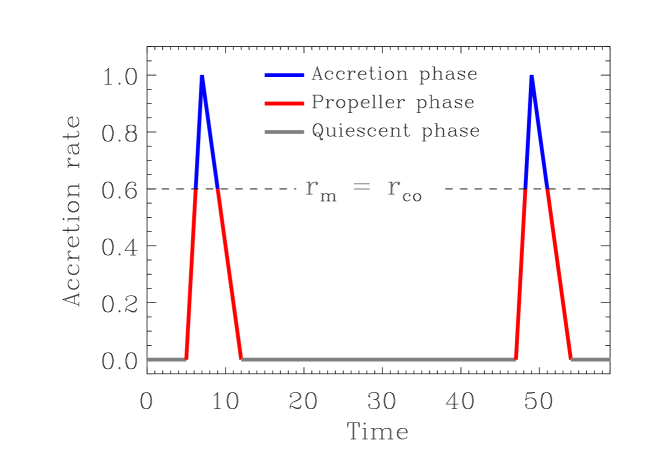
Figure 1: A schematic illustration of how the accretion rate $\dot{M}$ evolves through various phases for a transient LMXB. The instantaneous $\dot{M}$ is normalized by the outburst peak value $\dot{M}_{\rm max}$, and time is plotted in arbitrary units. Two outbursts are shown, with triangular outburst profiles, separated by a quiescent interval. The dashed horizontal line shows the condition $r_{\rm m}=r_{\rm co}$, which corresponds to the normalized effective accretion rate $\dot{M}_{\rm eff}/\dot{M}_{\rm max}$. When $\dot{M}$ is above this line, the source is in the accretion phase (blue). When $\dot{M}$ is below this line but within an outburst, the source is in the propeller phase (red). Outside of the two outbursts shown in the figure, the source is in the quiescent phase (grey).

For simplicity, we model the time evolution of a transient outburst as a linear increase of $\dot{M}$ from quiescence ($\dot{M}\simeq 0$) to a maximum value $\dot{M}_{\rm max}$, followed by a linear decrease of $\dot{M}$ back down to quiescence (Figure 1). In actuality, the magnitude of the rise and decay slopes can be different, although this does not affect our qualitative results. The evolution of $\dot{M}$ over an outburst causes $r_{\rm m}$ to change as well. As the outburst rises, the system moves from quiescence ($r_{\rm m}\simeq r_{\rm lc}$) through the propeller regime ($r_{\rm m}>r_{\rm co}$) into the accretion regime ($r_{\rm m}<r_{\rm co}$). During the decay, the systems passes back from accretion through propeller into quiescence. For an outburst duty cycle (fractional duration) $f$, we have

$$\dot{M}_{\rm av}\simeq\frac{1}{2}\,f\,\dot{M}_{\rm max},$$ (14)

independent of the recurrence time. It is convenient to define a transience parameter $\dot{m}=\dot{M}_{\rm max}/\dot{M}_{\rm av}$; this scales as $1/f$, with the proportionality factor depending on the shape of the outburst light curve. This factor is $1/2$ for the triangular outburst profiles we consider here.

2.3 Numerical computation of spin evolution

We wish to compare the spin evolution of persistent and transient accretors for the same average accretion rate $\dot{M}_{\rm av}$. In all cases, we start with a slowly spinning ($\nu\simeq 1$ Hz) neutron star with mass $M=1.35M_{\odot}$ (Thorsett & Chakrabarty, 1999), moment of inertia $I=0.4MR^{2}$ (Revnivtsev & Mereghetti, 2015), and a fixed surface magnetic field $B$. We then compute the spin evolution of the neutron star for a fixed $\dot{M}_{\rm av}$, using Equations 9 and 10, and continue until a certain total rest mass $\Delta M_{\rm tot}=0.6\,M_{\odot}$ is transferred to the neutron star. Note that the amount of mass transferred to a neutron star depends on the progenitor system (e.g., LMXB versus intermediate-mass X-ray binary (IMXB); Lin et al., 2011; Chen et al., 2016), and is not fully understood yet. While a transferred mass of $\sim 0.1M_{\odot}$ can make a neutron star fast-spinning (this paper; Tauris et al., 2013), a gravitational mass as high as $\sim 0.4M_{\odot}$ could also be transferred (Lin et al., 2011). Therefore, since the transferred rest mass is higher than the corresponding gravitational mass considering the binding energy (Bagchi, 2011), we continue our calculation until $0.6\,M_{\odot}$ rest mass is transferred, to be on the safe side. For the persistent case, we simply set the instantaneous accretion rate $\dot{M}=\dot{M}_{\rm av}$. For the transient case, we allow $\dot{M}$ to vary through a series of outbursts with transience parameter $\dot{m}$. The torques in Equations 9 and 10, along with the instantaneous $\dot{M}$, determine the amount of angular momentum $\Delta J$ and rest mass transferred in each time step. We account for the conversion of accreted rest mass to gravitational mass in the neutron star using Equations 19 and 20 of Cipolletta et al. (2015). Using the increased $M$, we update our values of $R$ ($\propto M^{-1/3}$; see, e.g., Ghosh, 2007) and $I$, and then proceed to the next time step. Note that our choices for this relations are not unique, and in general will depend upon the equation of state model assumed for the neutron star core. However, our qualitative results do not depend on our specific choices here.

We consider $\dot{M}_{\rm av}$ values ranging from $5\times 10^{14}$ to $3\times 10^{17}$ g s^-1, corresponding to $\sim 0.0004-0.25\,\dot{M}_{\rm Edd}$, where $\dot{M}_{\rm Edd}\simeq 1.2\times 10^{18}$ g s^-1 is the Eddington critical accretion rate for a 1.35 $M_{\odot}$ neutron star. We also consider transience parameters $\dot{m}$ in the 2–200 range. These ranges are realistic. For example, the estimated $\dot{M}_{\rm av}$ and $\dot{m}$ are $\approx 7\times 10^{14}$ g s^-1 and $\approx 40$ respectively for SAX J1808.4–3658, and are $\approx 3\times 10^{16}$ g s^-1 and $\approx 8$ respectively for 4U 1608–522 (assuming a $0.2$ efficiency of energy generation; Watts et al., 2008; Chakrabarty et al., 2003). Besides, we consider $B$ values in the range $3\times 10^{7}-10^{9}$ G. Note that $B$ is held fixed for any given run; we do not model accretion-induced field decay, but rather start with a fixed field strength that is already low (“post-decay”). We perform our runs both including and excluding the electromagnetic torque term in Equation 12 during quiescence.

3 Results

Our results for a typical numerical run are shown in Figure 2. For the persistent accretor case, the spin frequency rapidly reaches $\nu_{\rm eq}$ (Equation 11) and then tracks $\nu_{\rm eq}$ as it gradually evolves with increasing $M$. For clarity, we will call the persistent equilibrium spin $\nu_{\rm eq,per}$. We find that, even for the same $\dot{M}_{\rm av}$, the evolution for a transient accretor is very different. Since the instantaneous $\dot{M}$ varies between a low value and $\dot{M}_{\rm max}$ over each transient outburst, the instantaneous $\nu_{\rm eq}$ will also vary between a low value and $\nu_{\rm eq,max}$ ($\nu_{\rm eq}$ corresponding to $\dot{M}_{\rm max}$). The $\nu_{\rm eq,max}$ curve is shown near the top of the figure. The large swings in instantaneous $\nu_{\rm eq}$ occur on too short a time scale to plot in the figure. Moreover, the outbursts are each much too short to allow the spin $\nu$ to track these rapid swings in $\nu_{\rm eq}$. Instead, $\nu$ smoothly increases until it reaches, and then tracks, an effective equilibrium frequency $\nu_{\rm eq,eff}$ which is significantly larger than $\nu_{\rm eq,per}$ (but not quite as large as $\nu_{\rm eq,max}$). If we include an electromagnetic spin-down torque during quiescence, then the resulting $\nu_{\rm eq,eff}^{\rm EM}$ curve is somewhat below the $\nu_{\rm eq,eff}$ curve (and with a shallower slope), but still much above the curve for the persistent case.

Qualitatively, these results are quite general across all of our runs. Figure 3 shows examples for a range of $B$, $\dot{M}_{\rm av}$, and $\dot{m}=\dot{M}_{\rm max}/\dot{M}_{\rm av}$ to demonstrate the robustness of our results. Figures 3a and 3b, which are for $B=10^{8}$ G and $\dot{M}_{\rm av}=6.3\times 10^{15}$ g s^-1, show that $\nu_{\rm eq,max}$, $\nu_{\rm eq,eff}$ and $\nu_{\rm eq,eff}^{\rm EM}$ are lower for lower $\dot{m}$. The effect of EM torques is larger for higher $\dot{m}$, as seen in these figures, for two reasons: first, EM torque has a strong spin dependence ($\sim\nu^{3}$; Equation 12), and second, the fractional quiescence duration (during which the EM torque is active) decreases with $f$, and hence increases with $\dot{m}$ (see Equation 14). Figure 3c shows that all the spin frequencies are lower for a higher $B=10^{9}$ G. This is because the accretion disk does not penetrate as far into the magnetosphere, and hence the minimum possible $r_{\rm m}$ value is higher (Equation 1). However, $\nu_{\rm eq,eff}$ is still significantly larger than $\nu_{\rm eq,per}$ for this case. In Figure 3d, we consider a much lower $B=3\times 10^{7}$ G and a smaller $\dot{M}_{\rm av}$, and find that all our results from Figure 2 are still valid. Here, we also show that the gravitational wave torque (Equation 13) can bring down $\nu$ significantly (in this case, below the observed cut-off value of $\simeq 730$Hz), but $\nu$ is still much higher than $\nu_{\rm eq,per}$.

In order to examine the effect of the uncertainty in $\eta$ value (Equation 10), we compute spin evolution for $\eta=0.2,0.5$ and $1$, keeping other parameter values same (see Figure 4). This figure shows that not only the nature of spin evolution remains same for this wide range of $\eta$ values, but also quantitatively the curves are not very different from each other. For example, there is $\approx 12$% difference in $\nu$ values between $\eta=0.2$ and $\eta=1$, after $0.6M_{\odot}$ rest mass is added to the neutron star. Therefore, our general conclusion, that $\nu$ attains a higher value for transience for the same $\dot{M}_{\rm av}$, remains valid for the assumed large range of $\eta$ values. Moreover, for a lower value of $\eta$, the spin-down torque is lower (Equation 10), and hence the star acquires an even higher $\nu$.

Figure 5 confirms the above conclusions in a compact manner and for a wide range of $\dot{M}_{\rm av}$ and $\dot{m}$ values. This figure comprehensively shows that the more extreme the transient behavior is (larger $\dot{m}$), the faster a neutron star spins for a given $\Delta M_{\rm tot}(=0.6M_{\odot})$. This figure also shows that the effect of EM torques can be significant if $\nu$ or $\dot{m}$ has a high value.

4 Analytical calculation of equilibrium spin frequency for transients

Figures 2 and 3 show that a transient source attains the equilibrium spin frequency $\nu_{\rm eq,eff}$, which is several times higher than that ($\nu_{\rm eq}$) for a persistent source. It is also interesting to note that $\nu_{\rm eq,eff}$ and $\nu_{\rm eq,max}$ maintain a constant ratio, as shown by the horizontal part of the red dash-dot curve of Figure 6b. In this section, we will try to analytically understand these two new results. Moreover, the analytical expression for $\nu_{\rm eq}$ for persistent accretors (Equation 11) is widely used to understand the spin distribution of MSPs, even though most of the neutron star LMXBs are transients. It would, therefore, be preferable to find an analytical expression of $\nu_{\rm eq,eff}$ appropriate for transient accretors, which could then be used to better understand the spin evolution and distribution of MSPs, most of which evolved in transients.

The spin-equilibrium condition for a transient source is somewhat different from that for a persistent source. Here is the reason. A persistent source, when it reaches the spin equilibrium, is expected to always remain in the spin equilibrium, as the $r_{\rm m}=r_{\rm co}$ condition could continuously remain valid. This spin equilibrium frequency $\nu_{\rm eq}$, given in Equation 11, evolves with increasing $M$ (Section 3). On the other hand, $\dot{M}$, and hence $r_{\rm m}$, change drastically for a transient source during an outburst. As a result, the neutron star always gains angular momentum during the accretion phase (Equation 9) and loses angular momentum during the propeller phase (Equation 10). Therefore, unlike in the case of a persistent source, a spin equilibrium cannot not be established at every instant for a transient source, and $r_{\rm m}=r_{\rm co}$ is not the correct condition for spin equilibrium of transients, as $r_{\rm m}$ drastically evolves. A simple balance of the positive torque (Equation 9) with the negative torque (Equation 10) also does not work, because they cannot balance each other throughout an outburst, as $r_{\rm m}$ evolves. What could then be the criterion for the spin equilibrium of a transient accretor? Note that, although $\nu$ evolves throughout the two phases of a given outburst in a cyclic manner, this change is negligible, given that a typical outburst duration is very small compared to the spin-up timescale of a neutron star. Therefore, if no net angular momentum is added to the neutron star in an outburst cycle, the small cyclic change in $\nu$ during each outburst can be ignored. As a result, for time scales longer than an outburst duration, a spin equilibrium for transients can be established if the stellar angular momentum gain in the accretion phase cancels the stellar angular momentum loss in the propeller phase in every outburst cycle. This criterion, to the best of our knowledge, has not previously been used to calculate the spin equilibrium frequency for transients.

In order to analytically estimate the equilibrium spin frequency $\nu_{\rm eq,eff}$, we consider a simple but general torque formula

$$\frac{{\rm d}J}{{\rm d}t}=\pm A\dot{M}^{n},$$ (15)

where $J$ is the stellar angular momentum, $A$ is a positive constant, and the positive and negative signs correspond to $r_{\rm m}<r_{\rm co}$ and $r_{\rm m}>r_{\rm co}$ respectively. We use this torque formula, because torques given by Equations 9 and 10 are not simple enough for analytical calculations. However, before proceeding further, it is desirable to check if the form of the torque formula given in Equation 15 is reasonable, that is if it can be approximately constructed from Equations 9 and 10. In order to do this, we note that $N_{\rm field}$ tends to $\mu^{2}/3r_{\rm m}^{3}$ for $r_{\rm m}<<r_{\rm co}$ in the accretion phase, and $N_{\rm field}$ tends to $-\mu^{2}/3r_{\rm m}^{3}$ for $r_{\rm m}>>r_{\rm co}$ in the propeller phase (Equations 7 and 8). For other values of $r_{\rm m}$, $N_{\rm field}$ has a value in between these limiting values. Therefore, using Equations 7 and 8, one could approximately write,

$$N_{\rm field}=\pm\frac{\beta\mu^{2}}{3r_{\rm m}^{3}},$$ (16)

where $0\leq\beta\leq 1$, and the positive (negative) sign is for the accretion (propeller) phase. Similarly, using Equations 4 and 5, and for $\eta=1$, one can write,

$$N_{\rm acc}=\pm\dot{M}\sqrt{GMr_{\rm m}},$$ (17)

where the positive (negative) sign is for the accretion (propeller) phase. Therefore, using Equation 3, as well as Equations 16 and 17, the approximate torque can be written as

$$N=\pm\dot{M}\sqrt{GMr_{\rm m}}\pm\frac{\beta\mu^{2}}{3r_{\rm m}^{3}}.$$ (18)

Using the Equation 1, it is easy to verify that this torque formula is exactly of the form given in Equation 15 (for $n=6/7$). Moreover, a comparison between the blue solid and red dash-dot curves of Figure 6a shows that Equation 18 gives a spin evolution very similar to that given by Equations 9 and 10, with a quantitative difference at the level of a few percent. Note that, following Tauris (2012), we assume $\beta=1/3$ in Equation 18 for Figure 6a. However, this specific value of $\beta$ is only for demonstration, and the spin evolution curve changes at most by a few percent between $\beta=0$ and $\beta=1$. Therefore it is reasonable to proceed with the simple but general torque formula given by Equation 15, which is suitable to analytically estimate the equilibrium spin frequency $\nu_{\rm eq,eff}$. Note that this exercise will also be very useful to understand the results described in Section 3.

As mentioned earlier, the spin frequency attains the equilibrium value $\nu_{\rm eq,eff}$, if $\Delta J$ in the accretion phase ($r_{\rm m}<r_{\rm co}$) and $\Delta J$ in the propeller phase ($r_{\rm m}>r_{\rm co}$) during an outburst cancel each other. Here, using Equation 15,

$$\Delta J=\int{\rm d}J=\pm A\int\dot{M}^{n}{\rm d}t=\pm A_{1}\int\dot{M}^{n}{\rm d}\dot{M},$$ (19)

where ${\rm d}\dot{M}/{\rm d}t$, and hence $A_{1}=A/({\rm d}\dot{M}/{\rm d}t)$, are constants for a linear $\dot{M}$ profile during an outburst. Therefore the above mentioned requirement for $\nu=\nu_{\rm eq,eff}$ gives

$$\dot{M}_{\rm max}^{n+1}-\dot{M}_{\rm eff}^{n+1}=\dot{M}_{\rm eff}^{n+1}-\dot{M}_{\rm lc}^{n+1},$$ (20)

and hence

$$\frac{\dot{M}_{\rm max}}{\dot{M}_{\rm eff}}=2^{1/(n+1)},$$ (21)

where the effective accretion rate $\dot{M}_{\rm eff}$ corresponds to $r_{\rm m}=r_{\rm co}$, and we assume $\dot{M}_{\rm lc}$ corresponding to quiescence ($r_{\rm m}\simeq r_{\rm lc}$) is zero. Since the equilibrium spin frequency scales as $\nu_{\rm eq}\propto\dot{M}^{3/7}$ (Equation 11), we find

$$\frac{\nu_{\rm eq,eff}}{\nu_{\rm eq,max}}=2^{-3/(7(n+1))}.$$ (22)

Equation 22 gives an analytical expression of equilibrium spin frequency $\nu_{\rm eq,eff}$ for transient sources. This equation also shows why $\nu_{\rm eq,eff}/\nu_{\rm eq,max}$ is a constant, as shown in Figure 6b. We expect $\nu_{\rm eq,eff}/\nu_{\rm eq,max}\approx 0.85$ for the torque in Equation 15, with $n=6/7$. This expected value from our simple analytical calculation very well matches (within $4$%) with the value from our numerical computation with the approximate torque given in Equation 18 (Figure 6b). Even the constant $\nu_{\rm eq,eff}/\nu_{\rm eq,max}$ ratio from the numerical computation with the torques given in Equations 9 and 10 matches within $10$% with the analytical value of 0.85. Note that this matching is better for a lower value of $\eta$ in Equation 10. Therefore, our analytical results for a simple torque formula is valid for the realistic torques (Equations 9 and 10) with a small error of a few percent.

Finally, we analytically estimate the range of $\nu_{\rm eq,eff}/\nu_{\rm eq,per}$, i.e., the ratio of spin rates for transient and persistent accretors with the same $\dot{M}_{\rm av}$ value. For this, we consider a typical $\dot{M}_{\rm max}/\dot{M}_{\rm av}$ of $10-100$ (Burderi et al., 1999). Since $\nu_{\rm eq}\propto\dot{M}^{3/7}$ (Equation 11), this range of $\dot{M}_{\rm max}/\dot{M}_{\rm av}$ gives a $\approx 2.7-7.2$ range for $\nu_{\rm eq,max}/\nu_{\rm eq,per}$. Assuming $n=6/7$ in Equation 15, and hence, $\nu_{\rm eq,eff}/\nu_{\rm eq,max}=0.85$, we analytically estimate a $\sim 2-6$ range of $\nu_{\rm eq,eff}/\nu_{\rm eq,per}$. This is consistent with the numerically computed curves displayed in Figures 2 and 3.

5 Discussion of assumptions

We use $\xi=1$ in this paper, which is consistent with the expected range $\sim 0.5-1.4$ (Wang, 1996). Note that a different value of $\xi$ does not change our qualitative results, as $\nu_{\rm eq,per}$, $\nu_{\rm eq,max}$, and hence $\nu_{\rm eq,eff}$ scale with $\xi$ in the same way, i.e., $\propto\xi^{-3/2}$. Note that, for fixed values of the equilibrium spin frequency and other parameters, the magnetic field $B\propto\xi^{-7/4}$ (Equation 11). Consequently, in order to attain a measured $\nu$ value, the stellar magnetic field is to be lower for a higher value of $\xi$. Therefore, a value of $\xi$ different from $1$ will not change our conclusions, but our assumed $B$ values will be different.

We use a linear $\dot{M}$ profile during both outburst rise and decay, because this is the simplest and the cleanest profile for the demonstration of our results. In reality, both rise and decay profiles may be complex, can have several peaks, can have a somewhat flat top and may be difficult to fit with a simple function (see, e.g., Figure 2 of Yan & Yu, 2015). However, such a complex profile will not in general change our conclusions. For example, an exponential decay profile ($\dot{M}\propto\exp[{-t/\tau}]$ with time constant $\tau$) gives $\nu_{\rm eq,eff}/\nu_{\rm eq,max}=2^{-3/7n}$, which is 0.71 for $n=6/7$. Therefore, for a linear rise and an exponential decay profile, which is often seen, the value of $\nu_{\rm eq,eff}/\nu_{\rm eq,max}$ should be between 0.71 and 0.85 for $n=6/7$. For a profile having a flat top, $\nu_{\rm eq,eff}/\nu_{\rm eq,max}$ is expected to have a higher value.

Is it justified to keep $B$, $\dot{M}_{\rm av}$ and $\dot{M}_{\rm max}$ fixed in our calculation of evolution? We consider each parameter in turn. In the case of $B$, it is convenient to keep the parameter fixed in order to cleanly demonstrate the effect of transient accretion on the spin evolution. We note that $B$ likely decreases by orders of magnitude from an initial high value ($\sim 10^{12}$ G) on a time scale short compared to the LMXB lifetime (see, e.g, Page et al., 2000; Geppert & Rheinhardt, 2002; Lamb & Yu, 2005; Patruno et al., 2012a; Istomin & Semerikov, 2016), and hence the use of a fixed low post-decay $B$ value may be justified. We also find this with our numerical calculations of spin evolution for two initial $\nu$ values, 1 Hz and 100 Hz, keeping other parameter values same. By the time the star is spun up to 100 Hz, $B$ must decrease to a much lower value or else the star could not be spun up to this high $\nu$ value, and a further major decrease of the $B$ value is unlikely. Since we find that the spin evolution curves for both cases are very similar to each other, we conclude that a fixed $B$ value considered in numerical calculation does not have an impact on the general conclusions of this paper.

In the case of $\dot{M}_{\rm av}$, we hold the parameter fixed in order to separate out the effect of transient accretion from the much slower variation of $\dot{M}_{\rm av}$ due to binary evolution, which is also already a much better studied issue. We do not expect any slow evolution of $\dot{M}_{\rm av}$ to change the main findings of this paper. Finally, in the case of $\dot{M}_{\rm max}$, we hold this parameter fixed merely for the purpose of demonstration. In reality, $\dot{M}_{\rm max}$ varies (usually within a factor of 10; Yan & Yu, 2015), and depending on this, $\nu$ should track an average $\nu_{\rm eq,eff}$ (e.g., in between red dashed curves of Figures 3a and 3b). However, our conclusions are not affected by this.

6 Summary and implications

The main finding of this paper is that the spin rate of a transient LMXB pulsar attains a much higher value than that for a persistent LMXB with the same average accretion rate, usually even for less than $0.1M_{\odot}$ mass transferred to the neutron star. This is easily visible in Figures 2 and 3. This crucial effect of transient accretion on the spin-up of neutron stars implies that any meaningful study of the observed spin distribution of MSPs requires its inclusion. This effect will also have impact on the current understanding of spin-up and spin-down torques, accretion, binary evolution and $B$-values, because nearly all the accreting MSPs are transients.

In this paper, we also report, for the first time, an analytical expression of equilibrium spin frequency appropriate for transients. The standard expression of $\nu_{\rm eq}$ in persistent accretors (Equation 11) laid the foundation for previous pulsar spin distribution studies. However, this should now be replaced by our expression for $\nu_{\rm eq,eff}$ (Equation 22) for transients. Note that $\nu_{\rm eq,eff}$, unlike $\nu_{\rm eq}$, depends on the torque law, and hence may provide a way to better understand the interaction between the accretion disk and the pulsar magnetosphere.

Finally, Figures 2–6 show that at least some neutron stars with appropriate parameter values are expected to reach submillisecond spin rates, even for low $\dot{M}_{\rm av}$. Our results reemphasize the puzzling absence of observed MSPs with spin rates above 716 Hz and suggest a reconsideration of the need for a competing spin-down mechanism, such as gravitational radiation. Recent work concluding that the spin equilibrium set by disk-magnetosphere interaction alone is suffcient to explain the observed spin distribution (e.g., Patruno et al., 2012b) does not account for the effect of transient accretion, as we have shown here. Another recent paper Parfrey et al. (2016) proposes a new spin-down mechanism via an enhanced pulsar wind during the accretion phase, but again does not consider the effect of transient accretion. While it is generally believed that radio pulsar activity only switches on during an X-ray quiescence phase (Section 2.1), these authors argue that the neutron star magnetic field lines within the light cylinder can be forced to open to infinity by the accretion disk, which may give rise to a strong pulsar wind in the accretion phase. However, even if this possibility is confirmed, spin-down torques due to gravitational radiation may still play a role for the fastest rotating MSPs. This is not inconsistent with the absence of evidence for a gravitational wave torque in slower MSPs (Haskell & Patruno, 2011), considering the extremely steep spin dependence ($\sim\nu^{5}$; Equation 13) of such torques. The resulting continuous gravitational radiation may eventually itself be directly detectable with interferometric detectors (e.g., Aasi et al., 2014), although the practical obstacles to making such detections in transient LMXBs (where regular monitoring of the evolving binary parameters is difficult) have been previously discussed (Watts et al., 2008).

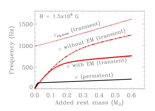
Figure 2: Numerically computed evolution of spin frequency versus transferred rest mass. We assume initial parameter values of gravitational mass $M=1.35M_{\odot}$ and $\nu=1$ Hz, and fixed parameter values of $B=1.5\times 10^{8}$ G and $\dot{M}_{\rm av}=6.3\times 10^{15}$ g s^-1 (i.e., $10^{-10}$ $M_{\odot}$/yr). The torques given in the Equations 9 and 10 (with $\eta=1$) are used. This figure compares the spin rate evolution between a transient and a persistent source for the same average accretion rate. The three upper curves (in red) are for a transient with the transience parameter $\dot{m}=\dot{M}_{\rm max}/\dot{M}_{\rm av}=100$. Among these, the dotted curve corresponds to the maximum possible equilibrium spin frequency $\nu_{\rm eq,max}$ (which is $\nu_{\rm eq}$ for $\dot{M}_{\rm max}$), the dash-dot curve corresponds to the spin frequency $\nu$ without considering the effect of EM torques, and the solid curve corresponds to the spin frequency $\nu$ including spin down due to EM torques. The lower curve (in black) is the spin frequency for a persistent accretor with $\dot{M}=\dot{M}_{\rm av}$. The nearly saturated value after the initial rise corresponds to the equilibrium spin frequency $\nu_{\rm eq,per}$ (which is $\nu_{\rm eq}$ for persistent accretion). Note that the persistent accretor needs only a small amount of transferred mass to attain $\nu_{\rm eq,per}$. This figure shows that the neutron star in a transient can spin up to a much higher value relative to that in a persistent source.

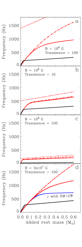
Figure 3: Numerically computed evolution of spin frequency as in Figure 2, for several different cases. Panel-a: same as in Figure 2, except with $B=10^{8}$ G. Panel-b: same as in panel-a, except with transience parameter $\dot{m}=10$. Panel-c: same as in panel-a, except with $B=10^{9}$ G. Panel-d: same as in panel-a, except with $B=3\times 10^{7}$ G and $\dot{M}_{\rm av}=1.2\times 10^{15}$ g s^-1 (i.e., $\approx 10^{-3}\,\dot{M}_{\rm Edd}$ for a 1.35 $M_{\odot}$ neutron star). The additional blue solid curve in this panel includes the spin down due to both EM and GW. This figure confirms the findings from Figure 2 for a wide range of parameter values.

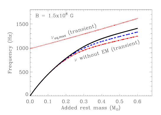
Figure 4: Numerically computed evolution of spin frequency as in Figure 2, for different $\eta$ values (see Equation 10; Section 2.1). Red dash-dot curve: $\eta=1$ (as in Figure 2); blue dashed curve: $\eta=0.5$; black solid curve: $\eta=0.2$. This figure shows that, even for drastically different $\eta$ values, the spin frequency evolutions are qualitatively similar to each other, and even quantitatively are not very different.

Figure 5: Spin-up efficiency (frequency increase per unit rest mass transfer) versus transience parameter $\dot{m}=\dot{M}_{\rm max}/\dot{M}_{\rm av}$, from numerical computation of spin evolution of accreting neutron stars. We assume initial parameter values of $M=1.35M_{\odot}$ and $\nu=1$ Hz and a fixed value of $B=1.5\times 10^{8}$ G. The solid curves with filled circles include the effect of spin-down due to EM torques, while the corresponding dotted curves with cross symbols do not. For each point (circle or cross), $\Delta M_{\rm tot}=0.6M_{\odot}$. Curves are for the following $\dot{M}_{\rm av}$ values: $5\times 10^{14}$, $10^{15}$, $5\times 10^{15}$, $10^{16}$, $5\times 10^{16}$, $10^{17}$, $3\times 10^{17}$ g s^-1 (bottom to top). The $\dot{m}$ values used are $2,3,5,10,20,30,50,100,200$ (left to right). However, not all of these $\dot{m}$ values are available for every $\dot{M}_{\rm av}$ value, since we do not consider accretion rates exceeding the Eddington limit. This figure shows that spin up efficiency increases with transience for reasonable $\dot{M}_{\rm av}$ and $\dot{m}$ ranges, even when spin-down due to EM torques is included.

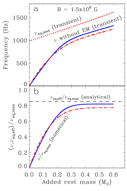
Figure 6: Numerically computed evolution of spin frequency as in Figure 2. Panel-a: The red dash-dot curve is for the realistic torques given by Equations 9 and 10, and the blue solid curve is for the approximate torque given by Equation 18. Both these curves show computed spin frequency $\nu$ evolution due to mass transfer. This panel shows that the spin evolution for the approximate torque is qualitatively similar to, and quantitatively only a few percent different from, that for the realistic torques. Panel-b: The red dash-dot and blue solid curves are same as in panel-a, except the $\nu$ values are normalized with $\nu_{\rm eq,max}$ (shown by the red dotted curve in panel-a). The dashed horizontal line gives a normalized (with $\nu_{\rm eq,max}$) analytical value of the equilibrium spin frequency $\nu_{\rm eq,eff}$, corresponding to Equation 22. This panel shows that both the red dash-dot and blue solid curves saturate as $\nu$ attains the equilibrium value $\nu_{\rm eq,eff}$. This numerical saturation value is close to the analytical value of $\approx 0.85$ from Equation 22 for $n=6/7$.

References

- Aasi et al. (2014) Aasi, J., Abadie, J., Abbott, B. P., et al. 2014, ApJ, 785, 119
- Alpar et al. (1982) Alpar, M. A., Cheng, A. F., Ruderman, M. A., & Shaham, J. 1982, Nature, 300, 728
- Andersson et al. (2005) Andersson, N., Glampedakis, K., Haskell, B., Watts, A. L. 2005, MNRAS, 361, 1153
- Andersson et al. (1999) Andersson, N., Kokkotas, K. D., Stergioulas, N. 1999, ApJ, 516, 307
- Archibald et al. (2009) Archibald, A. M., Stairs, I. H., Ransom, S. M., et al. 2009, Science, 324, 1411
- Bagchi (2011) Bagchi, M. 2011, MNRAS, 413, L47
- Bhattacharyya (2010) Bhattacharyya, S. 2010, Advances in Space Research, 45, 949
- Bhattacharyya et al. (2016) Bhattacharyya, S., Bombaci, I, Logoteta, D., Thampan, A. V. 2016, MNRAS, 457, 3101
- Bildsten (1998) Bildsten, L. 1998, ApJ, 501, L89
- Bogdanov et al. (2007) Bogdanov, S., Rybicki, G. B., & Grindlay, J. E. 2007, APJ, 670, 668
- Burderi et al. (1999) Burderi, L., Possenti, A., Colpi, M., et al. 1999, ApJ, 519, 285
- Chakrabarty (2005) Chakrabarty, D. 2005, in Binary Radio Pulsars, ed. F. A. Rasio and I. H. Stairs, (ASP Conference Series: San Francisco), 328, 279
- Chakrabarty (2008) Chakrabarty, D. 2008, AIP Conf. Proc., 1068, 67
- Chakrabarty & Morgan (1998) Chakrabarty, D., & Morgan, E. H. 1998, Nature, 394, 346
- Chakrabarty et al. (2003) Chakrabarty, D., Morgan, E. H., Muno, M. P., et al. 2003, Nature, 424, 42
- Chen et al. (2016) Chen, W.-C., & Podsiadlowski, P., 2016, ApJ, in press (arXiv:1608.02088)
- Cipolletta et al. (2015) Cipolletta, F., Cherubini, C., Filippi, S., et al. 2015, Phys. Rev. D, 92, 023007
- Cook et al. (1994) Cook, G. B., Shapiro, S. L., Teukolsky, S. A. 1994, ApJ, 424, 823
- D’Angelo & Spruit (2010) D’Angelo, C. R., & Spruit, H. C. 2010, MNRAS, 406, 1208
- de Martino et al. (2013) de Martino, D., Belloni, T., Falanga, M., et al. 2013, A&A, 550, A89
- Done et al. (2007) Done, C., Gierliński, M., & Kubota, A. 2007, ARA&A, 15, 1
- Ferrario & Wickramasinghe (2007) Ferrario, L., & Wickramasinghe, D. 2007, MNRAS, 375, 1009
- Geppert & Rheinhardt (2002) Geppert, U., Rheinhardt, M. 2002, A&A, 392, 1015
- Ghosh (2007) Ghosh, P. 2007, Rotation and Accretion Powered Pulsars,(World Scientific, New Jersey), pp. 177
- Ghosh & Lamb (1979) Ghosh, P., & Lamb, F. K. 1979, ApJ, 234, 296
- Hartman et al. (2008) Hartman, J. M., Patruno, A., Chakrabarty, D., et al. 2008, ApJ, 675, 1468
- Haskell & Patruno (2011) Haskell, B., & Patruno, A. 2011, ApJ, 738, L14
- Hessels (2008) Hessels, J. W. T. 2008, AIP Conf. Proc., 1068, 130
- Illarionov & Sunyaev (1975) Illarionov, A. F., & Sunyaev, R. A. 1975, A&A, 39, 185
- Istomin & Semerikov (2016) Istomin, Y. N., & Semerikov, I. A. 2016, MNRAS, 455, 1938
- Lamb & Yu (2005) Lamb, F. K., & Yu, W. 2005, in Binary Radio Pulsars, ed. F. A. Rasio & I. H. Stairs, (ASP Conference Series: San Francisco), 328, 299
- Lamb et al. (1973) Lamb, F. K., Pethick, C. J., & Pines, D. 1973, ApJ, 184, 271
- Lasota (1997) Lasota, J. P. 1997, in Accretion Phenomena and Related Outflows, ed. D. T. Wickramasinghe, L. Ferrario & G. V. Bicknell, (ASP Conference Series), 121, 351
- Lattimer & Prakash (2007) Lattimer, J. M., & Prakash, M. 2007, Phys. Rep., 442, 109
- Lin et al. (2011) Lin, J., Rappaport, S., Podsiadlowski, Ph., Nelson, L., Paxton, B., & Todorov, P. 2011, ApJ, 732, 70
- Linares (2014) Linares, M. 2014, ApJ, 795, 72
- Liu et al. (2013) Liu, Q. Z., van Paradijs, J., & van den Heuvel, E. P. J. 2013, A&A, 469, 807
- Livio & Pringle (1992) Livio, M., & Pringle, J. E. 1992, MNRAS, 259, 23
- Page et al. (2000) Page, D., Geppert, U., & Zannias, T. 2000, A&A, 360, 1052
- Papitto et al. (2013) Papitto, A., Ferrigno, C., Bozzo, E., et al. 2013, Nature, 501, 517
- Papitto et al. (2014) Papitto, A., Torres, D. F., Rea, N., Tauris, T. M. 2014, A&A, 566, A64
- Patruno (2010) Patruno, A. 2010, ApJ, 722, 909
- Patruno et al. (2012a) Patruno, A., Alpar, M. A., & van der Klis, M., et al. 2012a, ApJ, 752 33
- Patruno et al. (2012b) Patruno, A., Haskell, B., & D’Angelo, C. 2012b, ApJ, 746, 9
- Patruno & Watts (2012) Patruno, A., & Watts, A. L. 2012, in Timing neutron stars: pulsations, oscillations & explosions, ed. T. Belloni, M. Mendez & C. M. Zhang,(ASSL, Springer)
- Parfrey et al. (2016) Parfrey, K., Spitkovsky, A., & Beloborodov, A. M. 2016, ApJ, 822, 33
- Possenti et al. (1999) Possenti, A., Colpi, M., Geppert, U., Burderi, L., & D’Amico, N., 1999, ApJS, 125, 463
- Pringle & Rees (1972) Pringle, J. E., & Rees, M. J. 1972, A&A, 21, 1
- Psaltis & Chakrabarty (1999) Psaltis, D., & Chakrabarty, D. 1999, ApJ, 521, 332
- Radhakrishnan & Srinivasan (1982) Radhakrishnan, V., & Srinivasan, G. 1982, Current Science, 51, 1096
- Rappaport et al. (2004) Rappaport, S. A., Fregeau, J. M., & Spruit, H. 2004, ApJ, 606, 436
- Revnivtsev & Mereghetti (2015) Revnivtsev, M., & Mereghetti, S. 2015, Space Science Reviews, 191, 293
- Stella et al. (1994) Stella, L., Campana, S., Colpi, M., et al. 1994, ApJ, 423, L47
- Tauris (2012) Tauris, T. M. 2012, Science, 335, 561
- Tauris et al. (2013) Tauris, T. M., Kramer, M., & Langer, N., 2013, Proceedings of the International Astronomical Union, 291, 137
- Thorsett & Chakrabarty (1999) Thorsett, S. E., & Chakrabarty, D. 1999, ApJ, 512, 288
- Ustyugova et al. (2006) Ustyugova, G. V., Koldoba, A. V., Romanova, M. M., et al. 2006, ApJ, 646, 304
- Wang (1995) Wang, Y.-M 1995, ApJ, 449, L153
- Wang (1996) Wang, Y.-M 1996, ApJ, 465, L111
- Watts (2012) Watts, A. L. 2012, ARA&A, 50, 609
- Watts et al. (2008) Watts, A. L., Krishnan, B., Bildsten, L., Schutz, B. F. 2008, MNRAS, 389, 839
- Wijnands & van der Klis (1998) Wijnands, R., & van der Klis, M. 1998, Nature, 394, 344
- Yan & Yu (2015) Yan, Z., & Yu, W. 2015, ApJ, 805, 87