QoS-Based Linear Transceiver Optimization for Full-Duplex Multi-User Communications

Abstract

In this paper, we consider a multi-user wireless system with one full duplex (FD) base station (BS) serving a set of half duplex (HD) mobile users. To cope with the in-band self-interference (SI) and co-channel interference, we formulate a quality-of-service (QoS) based linear transceiver design problem. The problem jointly optimizes the downlink (DL) and uplink (UL) beamforming vectors of the BS and the transmission powers of UL users so as to provide both the DL and UL users with guaranteed signal-to-interference-plus-noise ratio performance, using a minimum UL and DL transmission sum power. The considered system model not only takes into account noise caused by non-ideal RF circuits, analog/digital SI cancellation but also constrains the maximum signal power at the input of the analog-to-digital converter (ADC) for avoiding signal distortion due to finite ADC precision. The formulated design problem is not convex and challenging to solve in general. We first show that for a special case where the SI channel estimation errors are independent and identically distributed, the QoS-based linear transceiver design problem is globally solvable by a polynomial-time bisection algorithm. For the general case, we propose a suboptimal algorithm based on alternating optimization (AO). The AO algorithm is guaranteed to converge to a Karush-Kuhn-Tucker solution. To reduce the complexity of the AO algorithm, we further develop a fixed-point method by extending the classical uplink-downlink duality in HD systems to the FD system. Simulation results are presented to demonstrate the performance of the proposed algorithms and the comparison with HD systems.

Keywords$-$ Beamforming, Full duplex system, Multi-user communications, Alternating optimization

EDICS: SAM-BEAM, SPC-INTF, SPC-APPL, SAM-APPL.

I Introduction

The next generation wireless communication systems target at ten times faster transmission rates and much shorter latency than the current 4G system. In addition to more powerful coding schemes and advanced multiple antenna techniques, the full duplex (FD) technique has also been considered as a solution with great potential to reach the target [2]. Ideally, a FD system can double the spectral efficiency compared to the conventional half duplex (HD) systems since it allows the node to transmit and receive signals at the same time and over the same frequency [3]. In practice, however, simultaneous transmission and reception cause severe self-interference (SI) which might greatly limit the system performance. Fortunately, recent advances in analog and digital SI cancellation (SIC) techniques have made the FD technique successfully implemented in bi-directional [4], relay [5] and WiFi [6, 7, 8] systems.

Recently, there have been of great interest to consider the FD techniques in the multi-user cellular systems [9]. Specifically, in such scenarios, a FD base station (BS) can serve both the downlink mobile users (DMUs) and uplink mobile users (UMUs) simultaneously. However, new challenges arise as not only the BS suffers from the SI, but also the DMUs are interfered by UMUs. This new form of uplink-to-downlink (UL-to-DL) co-channel interference (CCI) could become the performance bottleneck if not appropriately mitigated. In fact, the SI and UL-to-DL CCI couples the DL and UL transmissions, and therefore unlike the HD systems where the UL and DL transmissions can be designed separately, the FD system must consider a joint UL and DL transmission design. There have been considerable efforts studying the FD joint design problems in the literature; see, e.g., [10, 11, 12, 13, 14, 15, 16, 17]. Most of the works have focused on the multiple-input multiple-output (MIMO) scenarios by assuming that both the BS and MUs are equipped with multiple antennas. For example, [16, 11, 12, 13, 14] have studied beamforming/precoding and resource allocation algorithms for network sum rate or energy efficiency maximization, while [10, 17] have considered algorithms for providing the MUs with guaranteed quality-of-service (QoS).

In this paper, we consider a multiple-input single-output (MISO) scenario where each of the MUs has a single antenna. The multi-antenna FD BS employs transmit beamforming for DL transmission [18]. Unlike [16, 11, 12, 13, 14], which assumed the optimal non-linear receiver for UL signal detection, we consider a linear receive beamforming scheme for signal-user detection at the BS [18]. Under these settings, we formulate a QoS-based linear transceiver design problem that minimizes the sum of UL and DL transmission powers subject to constraints that guarantee minimum signal-to-interference-plus-noise ratio (SINR) requirement of MUs. Like the MIMO formulations considered in [16, 11, 12, 13, 14], the MISO QoS-based linear transceiver problem is still difficult to solve [17] due to the coupled DL and UL transmissions. We are interested in such problem formulation for two reasons. First, the QoS based formulation is more fundamental as the solution to the problem can be used for other design formulations such as the max-min-fairness designs [19] and rate region characterization. Second, in HD systems, the DL QoS-based beamforming problem [20] and UL QoS-based receive beamforming and power control problem [21] are known polynomial-time solvable, though they are not convex problems in their original forms. Specifically, there exists an uplink-downlink duality (UDD) [22, 23, 19] between the UL and DL problems and the two problems can be efficiently solved by a fixed-point iterative method [19, 22]. Therefore, it is interesting to see whether these elegant results can be generalized to the FD systems. The main contributions of this paper are threefold:

• Practical problem formulation: As motivated by the circuit designs in [24, 8, 7], we consider a system model that not only takes into account the noise caused by non-ideal RF chains but also the capability of analog and digital SIC schemes. The proposed formulation based on this practical model thus captures the impact of these relevant system parameters on the network performance. In particular, different from the existing works [10, 11, 12, 13, 14, 15, 16, 17], the formulated QoS-based design problem explicitly constrains the signal power level at the input of analog-to-digital converter (ADC), for avoiding signal distortion due to limited ADC precision. Such constraint is critical to the design of a FD transceiver [24], but has not been explicitly considered in the literature.

• Polynomial-time solvable subclass: While the QoS-based linear transceiver problem is non-convex and difficult to solve in general, we identify one intriguing case of the problem that is globally solvable. Specifically, we show that if the SI channel estimation error (i.e., the residual SI channel after analog SIC) has independent and identically distributed (i.i.d.) elements, then the non-convex problem can actually be globally solved by a bisection algorithm. The algorithm itself reveals interesting insights into the solution structure of the considered problem.

• Efficient suboptimal algorithm: In particular, our analysis suggests that it is unlikely to solve the QoS-based linear transceiver design problem in a convex fashion with respect to all the variables of the DL beamformer, UL beamformer and UMUs’ transmission powers. In light of this, to handle the considered design problem in general, we propose an alternating optimization (AO) based suboptimal algorithm, which iteratively optimizes the UL beamformer followed by optimizing the DL beamformer and UMUs’ transmission powers until convergence. Moreover, we generalize the UDD in HD systems [22, 23, 19] to the FD system and developed a new fixed-point algorithm to improve the computational efficiency of the proposed AO algorithm.

Simulation results are presented to illustrate the performance of the proposed algorithms under various settings and comparison with the HD system.

Synopsis: Section II presents the FD system model and the considered QoS-based design problem. Some existing results in HD systems are also briefly reviewed. Section III considers a special case of the considered problem and proposed a globally optimal bisection algorithm. In Section IV, an AO algorithm is proposed, and the UDD and fixed-point algorithm for the FD systems are presented. Simulation results are given in Section V and conclusions are drawn in Section VI.

Notations: ${\rm diag}({\bm{A}})$ is a diagonal matrix with its diagonal elements equal to the diagonal elements of matrix ${\bm{A}}$; ${\rm diag}(\{a_{i}\}_{i})$ and ${\rm diag}({\bm{a}})$, where ${\bm{a}}=[a_{1},\ldots,a_{m}]^{T}$, both represent a diagonal matrix with $a_{i}$’s being the diagonal elements; we also denote $|{\bm{a}}|^{2}=[|a_{1}|^{2},\ldots,|a_{m}|^{2}]^{T}$ ; ${\bm{e}}_{n}$ denotes the elementary vector with one in the $n$th entry and zero otherwise. ${\bm{a}}\succeq{\bm{b}}$ denotes element-wise inequality for vectors ${\bm{a}}$ and ${\bm{b}}$, while ${\bm{A}}\succeq(\succ){\bm{B}}$ means that ${\bm{A}}-{\bm{B}}$ is a positive semidefinite (positive definite) matrix. $\lambda_{\max}({\bm{A}})$ denotes the maximum eigenvalue of matrix ${\bm{A}}$. ${\rm vec}({\bm{A}})$ is a vector obtained by stacking the columns of ${\bm{A}}$. Finally, ${\bm{I}}_{n}$ denotes the $n$ by $n$ identity matrix and ${\mathbb{E}}(\cdot)$ denotes the statistical expectation operator.

II Signal Model and Problem Formulation

II-A FD Signal Model

As shown in Figure 1, we consider a wireless system with one BS and a set of $K$ DMUs and $L$ UMUs. The DMUs want to receive information signal from the BS whereas the UMUs want to transmit information signals to the BS. We assume that a FD BS, which is equipped with $N_{t}$ antennas ($N_{t}\geq 1$), is capable of communicating with the DMUs and UMLs at the same time and over a common spectrum. The DMUs and UMUs are assumed to be HD and have a single antenna.

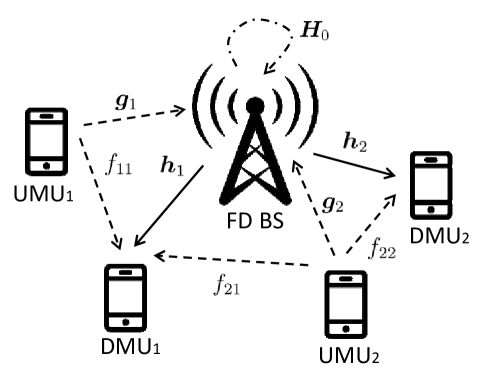
Figure 1: A wireless network with one FD BS and multiple MUs.

We present a FD signal model which is motivated by the circuit designs proposed in [24, 8] and the signal model in [4]. In particular, the proposed model explicitly accounts for the effects of analog SIC, digital SIC [24, 8] as well as transmitter and receiver noises caused by non-linear circuit components [4], which therefore allows for detailed assessment of the FD system performance. The proposed model is illustrated in Figure 2. Let ${\bm{x}}[n]=\sum_{i=1}^{K}{\bm{w}}_{i}s_{i}^{\rm D}[n]$ be the (discrete-time) signal transmitted by the BS to DMUs, where $s_{i}^{\rm D}[n]\in\mathbb{C}$ is the (independent, zero mean and unit power) information signal for DMU $i$, and ${\bm{w}}_{i}\in\mathbb{C}^{{N_{t}}}$ is the associated beamforming vector, for all $i\in{\mathcal{K}}\triangleq\{1,\ldots,K\}$. As shown in Figure 2, due to non-ideal transmitter RF chain (e.g., non-linearity of digital-to-analog converter (DAC) and power amplifier), the continuous-time information signal ${\bm{x}}(t)=\sum_{i=1}^{K}{\bm{w}}_{i}s_{i}^{\rm D}(t)$ is corrupted by a transmitter noise signal ${\bm{u}}_{\rm tx}(t)\in\mathbb{C}^{N_{t}}.$ Following [4], we model ${\bm{u}}_{\rm tx}(t)$ as a complex Gaussian random process with zero mean and covariance matrix $\beta_{1}{\rm diag}(\sum_{i=1}^{K}{\bm{w}}_{i}{\bm{w}}_{i}^{H})$ at each time $t$, i.e.,

$${\bm{u}}_{\rm tx}(t)\sim\mathcal{CN}\bigg{(}{\bm{0}},\beta_{1}{\rm diag}\bigg{(}\sum_{i=1}^{K}{\bm{w}}_{i}{\bm{w}}_{i}^{H}\bigg{)}\bigg{)},$$ (1)

​​where $\beta_{1}\ll 1$ is a constant. The noise ${\bm{u}}_{\rm tx}(t)$ is assumed to be independent of ${\bm{x}}(t)$ and the receiver noise. The combined signal ${\bm{x}}(t)+{\bm{u}}_{\rm tx}(t)$ is then transmitted to the DMUs through the antenna array.

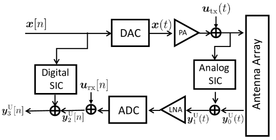
Figure 2: A block diagram of the transmitter and receiver chains of the FD BS.

II-A1 Downlink user SINR

Since the DMUs and UMUs communicate with the BS simultaneously, in addition to the signal from the BS, the DMUs also receive signals from the UMUs. Let ${\bm{h}}_{i}\in\mathbb{C}^{N_{t}}$ be the channel vector between the BS and the $i$th DMU, and let $f_{ji}\in\mathbb{C}$ be the channel coefficient from the UMU $j$ to DMU $i$ (see Figure 1). Moreover, denote $p^{\rm U}_{\ell}>0$ as the transmission power of the $\ell$th UMU, and $s_{\ell}^{\rm U}(t)\in\mathbb{C}$ as the (zero mean, unit power) UL information signal, for all $\ell\in{\mathcal{L}}\triangleq\{1,\ldots,L\}$. Then the received signal of each DMU $i$ is given by

$$y_{i}^{\rm D}(t) ={\bm{h}}_{i}^{H}\bigg{(}\sum_{k=1}^{K}{\bm{w}}_{k}s_{k}^{\rm D}(t)+{\bm{u}}_{\rm tx}(t)\bigg{)}+\sum_{j=1}^{L}f_{ji}\sqrt{p^{\rm U}_{j}}s_{j}^{\rm U}(t)+z^{\rm D}_{i}(t),~{}\forall i\in{\mathcal{K}},$$ (2)

where $z^{\rm D}_{i}(t)\in\mathbb{C}$ is the additive white Gaussian noise (AWGN) following $\mathcal{CN}(0,\sigma_{i}^{2})$. By (2), the SINR of DMU $i$ can be shown as

$${\rm SINR}_{i}^{\rm D}({\bm{W}},{\bm{p}}^{\rm U})=$$ (3)

$$\frac{|{\bm{h}}_{i}^{H}{\bm{w}}_{i}|^{2}}{\sum_{k\neq i}^{K}|{\bm{h}}_{i}^{H}{\bm{w}}_{k}|^{2}+\beta_{1}{\bm{h}}_{i}^{H}{\rm diag}(\sum_{k=1}^{K}{\bm{w}}_{k}{\bm{w}}_{k}^{H}){\bm{h}}_{i}+\hat{\sigma}_{i}^{2}({\bm{p}}^{\rm U})},$$

for all $i\in{\mathcal{K}}$, where ${\bm{W}}\triangleq[{\bm{w}}_{1},\ldots,{\bm{w}}_{K}]$, ${\bm{p}}^{\rm U}\triangleq[p_{1}^{\rm U},\ldots,p_{L}^{\rm U}]^{T}$ and $\hat{\sigma}_{i}^{2}({\bm{p}}^{\rm U})\triangleq\sum_{j=1}^{L}p_{j}^{\rm U}|f_{ji}|^{2}+\sigma_{i}^{2}.$ Note that the second and third terms in the denominator of (3) are due to the transmitter noise ${\bm{u}}_{\rm tx}(t)$, the UL-to-DL CCI $\sum_{j=1}^{L}f_{ji}\sqrt{p^{\rm U}_{j}}s_{j}^{\rm U}(t)$ and the additive noise. Let $\gamma^{\rm D}_{i}>0$ be the target SINR for DMU $i$. Then the SINR constraint for DMU $i$ can be written as

$${\rm SINR}_{i}^{\rm D}({\bm{W}},{\bm{p}}^{\rm U})\geq\gamma^{\rm D}_{i}$$

$$\Longleftrightarrow~{}~{} \frac{|{\bm{h}}_{i}^{H}{\bm{w}}_{i}|^{2}/\rho_{i}^{\rm D}}{\sum_{k=1}^{K}{\bm{w}}_{k}^{H}\tilde{}{\bm{H}}_{i}{\bm{w}}_{k}+\hat{\sigma}_{i}^{2}({\bm{p}}^{\rm U})}\geq 1,$$ (4)

where $\tilde{}{\bm{H}}_{i}\triangleq{\bm{h}}_{i}{\bm{h}}_{i}^{H}+\beta_{1}{\rm diag}(|{\bm{h}}_{i}|^{2}),$ for all $i\in{\mathcal{K}}$, and $\frac{1}{\rho_{i}^{\rm D}}\triangleq 1+1/\gamma_{i}^{\rm D}$.

II-A2 Uplink user SINR

Denote ${\bm{H}}_{0}\in\mathbb{C}^{N_{t}\times N_{t}}$ as the SI channel matrix and ${\bm{g}}_{\ell}\in\mathbb{C}^{N_{t}}$ as the channel vector from the $\ell$th UMU to the BS (see Figure 1). The signal received by the BS thus can be expressed as

$$\!\!\!\!\!{\bm{y}}^{\rm U}_{0}(t)=\sum_{\ell=1}^{L}{\bm{g}}_{\ell}\sqrt{p^{\rm U}_{\ell}}s_{\ell}^{\rm U}(t)+{\bm{H}}_{0}({\bm{x}}(t)+{\bm{u}}_{\rm tx}(t))+{\bm{z}}^{\rm U}(t),$$ (5)

where the second term in the right hand side (RHS) is the SI and the third term ${\bm{z}}^{\rm U}(t)$ is the AWGN following $\mathcal{CN}({\bm{0}},\sigma_{z}^{2}{\bm{I}}_{N_{t}})$. The SI power is in general much stronger than the signals transmitted from the UMUs and the AWGN, and therefore the SI has to be suppressed in order to decode the desired information data properly. However, simply mitigating the SI in the digital domain is insufficient. In fact, the SI power could be so large such that the receiver RF chain gets saturated as the dynamics of ${\bm{y}}^{\rm U}_{0}(t)$ may be out of the range that the ADC can support [24]. In view of this, SIC has to be carried out in the analog domain before ADC [24], as shown in Figure 2. Let ${\bm{H}}_{0}=\hat{}{\bm{H}}_{0}+{\bf\Phi}_{0}$, where $\hat{}{\bm{H}}_{0}$ and ${\bf\Phi}_{0}$ respectively represent the channel estimate of ${\bm{H}}_{0}$ and the associated estimation error matrix. Suppose that the analog SIC subtracts the estimated SI signal $\hat{}{\bm{H}}_{0}({\bm{x}}(t)+{\bm{u}}_{\rm tx}(t))$ from ${\bm{y}}^{\rm U}_{0}(t)$. Then the signal before ADC is given by

$$\!\!\!\!{\bm{y}}^{\rm U}_{1}(t)=\sum_{\ell=1}^{L}{\bm{g}}_{\ell}\sqrt{p^{\rm U}_{\ell}}s_{\ell}^{\rm U}(t)+{\bf\Phi}_{0}({\bm{x}}(t)+{\bm{u}}_{\rm tx}(t))+{\bm{z}}^{\rm U}(t).$$ (6)

After ADC, we obtain the following discrete-time signal

$${\bm{y}}^{\rm U}_{2}[n]= \sum_{\ell=1}^{L}{\bm{g}}_{\ell}\sqrt{p^{\rm U}_{\ell}}s_{\ell}^{\rm U}[n]+{\bf\Phi}_{0}({\bm{x}}[n]+{\bm{u}}_{\rm tx}[n])$$

$$+{\bm{u}}_{\rm rx}[n]+{\bm{z}}^{\rm U}[n].$$ (7)

Here, ${\bm{u}}_{\rm rx}[n]$ is the noise caused by the non-ideal receiver RF chain and follows

$${\bm{u}}_{\rm rx}[n]\sim\mathcal{CN}({\bm{0}},\beta_{2}{\rm diag}({\mathbb{E}}[{\bm{y}}^{\rm U}_{1}[n]({\bm{y}}^{\rm U}_{1}[n])^{H}])),$$ (8)

where $\beta_{2}\ll 1$ [4]. Before data detection, digital SIC is further carried out for ${\bm{y}}^{\rm U}_{2}[n]$. According to [8, 24], it is possible to suppress the linear SI components ${\bf\Phi}_{0}{\bm{x}}[n]$ and non-linear components ${\bf\Phi}_{0}{\bm{u}}_{\rm tx}[n]+{\bm{u}}_{\rm rx}[n]$ separately. For simplicity, we model that the linear SI power can be reduced by a factor of $\delta_{1}\ll 1$ and the non-linear SI power can be reduced by a factor of $\delta_{2}\ll 1$, due to the digital SIC. Therefore, the signal at the output of the digital SIC is given by

$${\bm{y}}^{\rm U}_{3}[n]= \sum_{\ell=1}^{L}{\bm{g}}_{\ell}\sqrt{p^{\rm U}_{\ell}}s_{\ell}^{\rm U}[n]+\sqrt{\delta_{1}}{\bf\Phi}_{0}{\bm{x}}[n]$$

$$+\sqrt{\delta_{2}}({\bf\Phi}_{0}{\bm{u}}_{\rm tx}[n]+{\bm{u}}_{\rm rx}[n])+{\bm{z}}^{\rm U}[n].$$ (9)

To detect $s_{\ell}^{\rm U}[n]$, the BS applies a linear receive beamformer, denoted by ${\bm{v}}_{\ell}\in\mathbb{C}^{{MN_{R}}}$, to ${\bm{y}}_{3}^{\rm U}[n]$, for all $\ell\in{\mathcal{L}}$. The SINR at the output of beamformer for UMU $\ell$ is thus given by

$${\rm SINR}_{\ell}^{\rm U}({\bm{W}},{\bm{p}}^{\rm U},{\bm{v}}_{\ell})=$$

$$\frac{p_{\ell}^{\rm U}|{\bm{v}}_{\ell}^{H}{\bm{g}}_{\ell}|^{2}}{\sum_{j\neq\ell}^{L}p_{j}^{\rm U}|{\bm{v}}_{\ell}^{H}{\bm{g}}_{j}|^{2}+{\bm{v}}_{\ell}^{H}{\mathbb{E}}[{\bf\Sigma}({\bm{W}},{\bf\Phi}_{0})]{\bm{v}}_{\ell}+\sigma_{z}^{2}\|{\bm{v}}_{\ell}\|_{2}^{2}},$$ (10)

where

$${\bm{v}}_{\ell}^{H}{\mathbb{E}}[{\bf\Sigma}({\bm{W}},{\bf\Phi}_{0})]{\bm{v}}_{\ell}\triangleq ~{}\delta_{1}{\bm{v}}_{\ell}^{H}{\mathbb{E}}[{\bf\Phi}_{0}{\bm{x}}(t){\bm{x}}^{H}(t){\bf\Phi}_{0}^{H}]{\bm{v}}_{\ell}$$

$$+\delta_{2}{\bm{v}}_{\ell}^{H}{\mathbb{E}}[{\bf\Phi}_{0}{\bm{u}}_{\rm tx}[n]{\bm{u}}_{\rm tx}^{H}[n]{\bf\Phi}_{0}^{H}]{\bm{v}}_{\ell}+\delta_{2}{\bm{v}}_{\ell}^{H}{\mathbb{E}}[{\bm{u}}_{\rm rx}[n]{\bm{u}}_{\rm rx}^{H}[n]]{\bm{v}}_{\ell}.$$ (11)

It is shown in Appendix A that (II-A2) can be compactly expressed as

$${\bm{v}}_{\ell}^{H}{\mathbb{E}}[{\bf\Sigma}({\bm{W}},{\bf\Phi}_{0})]{\bm{v}}_{\ell} =(\delta_{2}\beta_{2}){\bm{v}}_{\ell}^{H}\bigg{(}\sum_{j=1}^{L}p^{\rm U}_{j}{\rm diag}(|{\bm{g}}_{j}|^{2})\bigg{)}{\bm{v}}_{\ell}+{\bm{v}}_{\ell}^{H}{\bm{\Omega}}({\bm{W}},{\bm{R}}_{\Phi_{0}}){\bm{v}}_{\ell},$$ (12)

$$=(\delta_{2}\beta_{2}){\bm{v}}_{\ell}^{H}\bigg{(}\sum_{j=1}^{L}p^{\rm U}_{j}{\rm diag}(|{\bm{g}}_{j}|^{2})\bigg{)}{\bm{v}}_{\ell}+\sum_{k=1}^{K}{\bm{w}}_{k}^{H}{\bf\Lambda}({\bm{v}}_{\ell},{\bm{R}}_{\Phi_{0}}){\bm{w}}_{k},$$ (13)

​​using the matrices ${\bm{\Omega}}({\bm{W}},{\bm{R}}_{\Phi_{0}})$ and ${\bf\Lambda}({\bm{v}}_{\ell},{\bm{R}}_{\Phi_{0}})$ defined in (A) and (A.8), where ${\bm{R}}_{\Phi_{0}}\triangleq{\mathbb{E}}[{\rm vec}({\bf\Phi}_{0}){\rm vec}^{H}({\bf\Phi}_{0})]$ is the correlation matrix of vectorized ${\bf\Phi}_{0}$. Let us define

$$\tilde{}{\bm{G}}_{j}\triangleq{\bm{g}}_{j}{\bm{g}}_{j}^{H}+\delta_{2}\beta_{2}{\rm diag}(|{\bm{g}}_{j}|^{2}),$$ (14)

$$\tilde{\sigma}_{z}^{2}\triangleq(1+\delta_{2}\beta_{2})\sigma_{z}^{2},$$ (15)

and let $\gamma^{\rm U}_{\ell}>0$ be the SINR target of UMU $\ell$ for all $\ell\in{\mathcal{L}}$. Then either using (12) or (13), the SINR constraint ${\rm SINR}_{\ell}^{\rm U}\geq\gamma^{\rm U}_{\ell}$ for UMU $\ell$ can be written as

$${\rm SINR}_{\ell}^{\rm U}({\bm{W}},{\bm{p}}^{\rm U},{\bm{v}}_{\ell})\geq\gamma^{\rm U}_{\ell}$$

$$\Leftrightarrow\frac{p_{\ell}^{\rm U}|{\bm{v}}_{\ell}^{H}{\bm{g}}_{\ell}|^{2}/\rho_{\ell}^{\rm U}}{\sum_{j=1}^{L}p_{j}^{\rm U}{\bm{v}}_{\ell}^{H}\tilde{}{\bm{G}}_{j}{\bm{v}}_{\ell}+{\bm{v}}_{\ell}^{H}{\bm{\Omega}}({\bm{W}},{\bm{R}}_{{\bf\Phi}_{0}}){\bm{v}}_{\ell}+\tilde{\sigma}_{z}^{2}\|{\bm{v}}_{\ell}\|_{2}^{2}}\geq 1,$$ (16)

$$\Leftrightarrow\frac{p_{\ell}^{\rm U}|{\bm{v}}_{\ell}^{H}{\bm{g}}_{\ell}|^{2}/\rho_{\ell}^{\rm U}}{\sum_{j=1}^{L}p_{j}^{\rm U}{\bm{v}}_{\ell}^{H}\tilde{}{\bm{G}}_{j}{\bm{v}}_{\ell}+\sum_{k=1}^{K}{\bm{w}}_{k}^{H}{\bf\Lambda}({\bm{v}}_{\ell},{\bm{R}}_{{\bf\Phi}_{0}}){\bm{w}}_{k}+\tilde{\sigma}_{z}^{2}\|{\bm{v}}_{\ell}\|_{2}^{2}}\geq 1,$$ (17)

​​where $\frac{1}{\rho_{\ell}^{\rm U}}\triangleq 1+1/\gamma_{\ell}^{\rm U}$. It will be seen shortly that both formulations in (16) and (17) are useful in the development of the proposed algorithms.

II-A3 Constraint on ADC Input Signal Power

As mentioned, the signal dynamics should not be out of the range that the ADC can support as, otherwise, signal distortion can occur. Therefore, it is required to constrain the signal power of ${\bm{y}}_{1}^{\rm U}(t)$ at the input of the ADC. Let $\gamma^{\rm ADC}>0$ denote the maximum tolerable ADC input signal power. The ADC power constraint for the receiver RF chains are given by

$$\!\!\!\!\!\!{\rm ADC}({\bm{W}},{\bm{p}}^{\rm U})\triangleq{\rm diag}({\mathbb{E}}\{{\bm{y}}_{1}^{\rm U}(t)({\bm{y}}_{1}^{\rm U}(t))^{H}\})\!\!\preceq\!\gamma^{\rm ADC}{\bm{I}}_{N_{t}}.$$ (18)

It can be shown that, for $n=1,\ldots,N_{t},$

$$[{\rm ADC}({\bm{W}},{\bm{p}}^{\rm U})]_{n,n}={\bm{e}}_{n}^{T}{\mathbb{E}}\{{\bf\Phi}_{0}{\bm{W}}{\bm{W}}^{H}{\bf\Phi}_{0}^{H}\}{\bm{e}}_{n}$$

$$+\beta_{1}{\bm{e}}_{n}^{T}{\mathbb{E}}\{{\bf\Phi}_{0}{\rm diag}({\bm{W}}{\bm{W}}^{H}){\bf\Phi}_{0}^{H}\}{\bm{e}}_{n}+\sum_{j=1}^{L}p_{j}^{\rm U}|{\bm{e}}_{n}^{T}{\bm{g}}_{j}|^{2}+\sigma_{z}^{2},$$

$$=\sum_{k=1}^{K}{\bm{w}}_{k}^{H}{\bm{\Upsilon}}_{n}(\{{\bm{R}}_{\Phi_{0},m}\}){\bm{w}}_{k}+\sum_{j=1}^{L}p_{j}^{\rm U}|{\bm{e}}_{n}^{T}{\bm{g}}_{j}|^{2}+\sigma_{z}^{2},$$ (19)

where ${\bm{\Upsilon}}_{n}(\{{\bm{R}}_{\Phi_{0},m}\})\triangleq\bar{}{\bm{R}}_{\Phi_{0},n}+\beta_{1}{\rm diag}(\{{\bm{e}}_{n}^{T}{\bm{R}}_{\Phi_{0},m}{\bm{e}}_{n}\}_{m})$, and $\bar{}{\bm{R}}_{\Phi_{0},n}$ and ${\bm{R}}_{\Phi_{0},m}$ are defined in (A.9).

II-B Proposed Problem Formulation

Our goal is to design the UL transmission powers $\{p_{\ell}^{\rm U}\}$ and UL and DL beamformers $\{{\bm{v}}_{\ell}\}$, $\{{\bm{w}}_{k}\}$ so that the transmission power of the network (including the BS and the UMUs) is minimized subject to user SINR constraints and the ADC input power constraint. Mathematically, the QoS-based linear transceiver design problem is formulated as follows

$${\sf(P)}~{}~{}~{}\min_{\begin{subarray}{c}\{{\bm{w}}_{k}\},\{{\bm{v}}_{\ell}\},\\ \{p_{\ell}^{\rm U}\geq 0\}\end{subarray}}~{} \sum_{k=1}^{K}\|{\bm{w}}_{k}\|_{2}^{2}+\sum_{\ell=1}^{L}p_{\ell}^{\rm U}$$ (20a)

$${\rm s.t.}~{}~{} {\rm SINR}_{i}^{\rm D}({\bm{W}},{\bm{p}}^{\rm U})\geq\gamma^{\rm D}_{i},~{}i\in{\mathcal{K}},$$ (20b)

$${\rm SINR}_{\ell}^{\rm U}({\bm{W}},{\bm{p}}^{\rm U},{\bm{v}}_{\ell})\geq\gamma^{\rm U}_{\ell},~{}\ell\in{\mathcal{L}},$$ (20c)

$${\rm ADC}({\bm{W}},{\bm{p}}^{\rm U})\preceq\gamma^{\rm ADC}{\bm{I}}_{N_{t}},$$ (20d)

$$\|{\bm{v}}_{\ell}\|_{2}=1,~{}\ell\in{\mathcal{L}}.$$ (20e)

Unfortunately, problem (P) is non-convex and difficult to solve. Specifically, the UL SINR constraints and DL SINR constraints are coupled with each other due to the FD BS, which makes (P) drastically different from the traditional design problems in HD systems [18]. In subsequent sections, we present two methods to handle (P). Firstly, we show that for a special case of (P), the problem is globally solvable in a polynomial-time complexity. Secondly, for general (P), we propose an efficient AO method to solve it approximately.

II-C Review of Half-Duplex BF Solutions

Before studying the methods for solving the FD design problem (P), let us review some existing results about the QoS-based design problems in a HD system. These results will be used in the development of the proposed methods for solving (P).

In the HD system, the BS serves the DMUs and UMUs separately, either in different time slots or over distinct frequency bands. Thus, there is no SI (i.e., the term $\sum_{k=1}^{K}{\bm{w}}_{k}^{H}{\bf\Lambda}({\bm{v}}_{\ell},{\bf\Phi}_{0}){\bm{w}}_{k}$ in (17)) and no UL-to-DL CCI (i.e., the term $\sum_{j=1}^{L}p_{j}^{\rm U}|f_{ji}|^{2}$ in (II-A1)). The ADC input power constraint is also not necessary as the signal power at the input of ADC is generally small in the absence of SI. Therefore, the DL design problem (HD-DL)

$$\min_{\{{\bm{w}}_{k}\}}~{} \sum_{k=1}^{K}\|{\bm{w}}_{k}\|_{2}^{2}$$ (21a)

$${\rm s.t.}~{}~{} \frac{|{\bm{h}}_{i}^{H}{\bm{w}}_{i}|^{2}/\rho_{i}^{\rm D}}{\sum_{k=1}^{K}{\bm{w}}_{k}^{H}\tilde{}{\bm{H}}_{i}{\bm{w}}_{k}+\sigma_{i}^{2}}\geq 1,~{}k\in{\mathcal{K}},$$ (21b)

and UL design problem (HD-UL)

$$\min_{\{{\bm{v}}_{\ell}\},\{p_{\ell}^{\rm U}\geq 0\}}~{} \sum_{\ell=1}^{L}p_{\ell}^{\rm U}$$ (22a)

$${\rm s.t.}~{}~{} \frac{p_{\ell}^{\rm U}|{\bm{v}}_{\ell}^{H}{\bm{g}}_{\ell}|^{2}/\rho_{\ell}^{\rm U}}{\sum_{j=1}^{L}p_{j}^{\rm U}{\bm{v}}_{\ell}^{H}{\bm{g}}_{j}{\bm{g}}_{j}^{H}{\bm{v}}_{\ell}+\sigma_{z}^{2}\|{\bm{v}}_{\ell}\|_{2}^{2}}\geq 1,$$ (22b)

$$\|{\bm{v}}_{\ell}\|_{2}=1,~{}\ell\in{\mathcal{L}},$$ (22c)

can respectively be deduced from (P), and optimized independently [18].

While both (HD-DL) and (HD-UL) appear non-convex problems, it is well known that both of them own certain hidden convexity and can be globally solved in a polynomial-time complexity. Specifically, (HD-UL) is shown equivalent to a convex semidefinite program (SDP).

Lemma 1

[21] Suppose that (HD-UL) is feasible. Then (HD-UL) is equivalent to the following SDP

$$\max_{\{p_{\ell}^{\rm U}\geq 0\}}~{} \sum_{\ell=1}^{L}p_{\ell}^{\rm U}$$ (23)

$${\rm s.t.}~{}~{} \sum_{j=1}^{L}p_{j}^{\rm U}{\bm{g}}_{j}{\bm{g}}_{j}^{H}+\sigma_{z}^{2}{\bm{I}}_{N_{t}}\succeq\bigg{(}\frac{p_{\ell}^{\rm U}}{\rho_{\ell}^{\rm U}}\bigg{)}{\bm{g}}_{\ell}{\bm{g}}_{\ell}^{H},~{}\forall\ell\in{\mathcal{L}},$$

and therefore (HD-UL) is polynomial-time solvable.

Lemma 2

[21, Proposition 3.1][25] Suppose that (HD-UL) is feasible. The optimal power solution of problem (HD-UL) is unique and satisfies

$$\bigg{(}\frac{p_{\ell}^{\rm U}}{\rho_{\ell}^{\rm U}}\bigg{)}{\bm{g}}_{\ell}^{H}\bigg{(}\sum_{j=1}^{L}p_{j}^{\rm U}{\bm{g}}_{j}{\bm{g}}_{j}^{H}+\sigma_{z}^{2}{\bm{I}}_{N_{t}}\bigg{)}^{-1}{\bm{g}}_{\ell}=1,~{}\forall\ell\in{\mathcal{L}}.$$ (24)

The optimal beamformers are given by

$$\!\!\!\!{\bm{v}}_{\ell}=\frac{{\bm{v}}_{\ell}}{\|{\bm{v}}_{\ell}\|},\tilde{}{\bm{v}}_{\ell}=\bigg{(}\sum_{j=1}^{L}p_{j}^{\rm U}{\bm{g}}_{j}{\bm{g}}_{j}^{H}+\sigma_{z}^{2}{\bm{I}}_{N_{t}}\bigg{)}^{-1}{\bm{g}}_{\ell},~{}\forall\ell\in{\mathcal{L}}.$$ (25)

In fact, it can be verified that at the optimum, constraint (22b) must hold with equality, which leads to (24). Thus, Lemma 2 says that the $L$ nonlinear system of equations of (24) has a unique solution, uniquely determined by ${\bm{g}}_{j}$’s, ${\bm{g}}_{\ell}$’s, $\gamma_{\ell}^{\rm U}$’s and $\sigma_{z}^{2}$. Moreover, the optimal $\{p_{\ell}^{\rm U}\}$ can be obtained by solving equations (24) using a fixed-point method [22, 19].

The DL problem (HD-DL) can be solved by considering an equivalent second-order cone program (SOCP) [19] or a SDP [20] which is obtained by a semidefinite relaxation (SDR) technique [26]. Both SOCP and SDP are convex problems and are efficiently solvable by off-the-shelf solvers. The fixed-point method for UL problems can also be used to solve the DL problem (HD-DL), through a powerful UDD [27, 19, 18].

Lemma 3

[18] Suppose that (HD-DL) is feasible. (HD-DL) has a virtual UL counterpart as follows

$$\min_{\{\tilde{}{\bm{w}}_{i}\},\{\lambda_{i}\geq 0\}}~{} \sum_{i=1}^{K}\lambda_{i}\sigma_{i}^{2}$$ (26a)

$${\rm s.t.}~{}~{} \frac{\lambda_{i}|\tilde{}{\bm{w}}_{i}^{H}{\bm{h}}_{i}|^{2}/\rho_{i}^{\rm D}}{\sum_{k=1}^{K}\lambda_{k}\tilde{}{\bm{w}}_{i}^{H}\tilde{}{\bm{H}}_{k}\tilde{}{\bm{w}}_{i}+\|\tilde{}{\bm{w}}_{i}\|_{2}^{2}}\geq 1,$$ (26b)

$$\|\tilde{}{\bm{w}}_{i}\|_{2}=1,~{}i\in{\mathcal{K}},$$ (26c)

which has the same optimal objective value as (HD-DL).

In Section IV-B, we will show that such UDD can be generalized to the FD system.

III Optimal Solution for (P) with i.i.d. SI Channel Estimation Error

In this section, we consider a special case of (P) by assuming that elements of the SI channel estimation error are i.i.d. Specifically, ${\bm{R}}_{\Phi_{0}}$ is assumed to be ${\bm{R}}_{\Phi_{0}}=\sigma_{\Phi_{0}}^{2}{\bm{I}}_{N_{t}^{2}}$ for some $\sigma_{\Phi_{0}}^{2}>0$. Under this assumption, one can show that ${\bm{\Omega}}({\bm{W}},{\bm{R}}_{{\bf\Phi}_{0}})$ in the denominator of (16) reduces to $\xi\sum_{i=1}^{K}\|{\bm{w}}_{i}\|_{2}^{2}{\bm{I}}_{N_{t}}$, where $\xi\triangleq(\delta_{1}+\delta_{2}\beta_{1}+\delta_{2}\beta_{2}(1+\beta_{1}))\sigma_{\Phi_{0}}^{2}$, and ${\bm{\Upsilon}}_{n}(\{{\bm{R}}_{\Phi_{0},m}\})$ in the ADC input power constraint (19) reduces to ${\bm{\Upsilon}}_{n}(\{{\bm{R}}_{\Phi_{0},m}\})=\sigma_{\Phi_{0}}^{2}(1+\beta_{1})\sum_{i=1}^{K}\|{\bm{w}}_{i}\|_{2}^{2}{\bm{I}}_{N_{t}}$. As a result, problem (P) simplifies to

$${\sf(P1)}~{} \min_{\begin{subarray}{c}\{{\bm{w}}_{k}\},\{{\bm{v}}_{\ell}\},\\ \{p_{\ell}^{\rm U}\geq 0\}\end{subarray}}~{}\sum_{k=1}^{K}\|{\bm{w}}_{k}\|_{2}^{2}+\sum_{\ell=1}^{L}p_{\ell}^{\rm U}$$ (27a)

$${\rm s.t.}~{}~{} \frac{|{\bm{h}}_{i}^{H}{\bm{w}}_{i}|^{2}/\rho_{i}^{\rm D}}{\sum_{k=1}^{K}{\bm{w}}_{k}^{H}\tilde{}{\bm{H}}_{i}{\bm{w}}_{k}+\hat{\sigma}_{i}^{2}({\bm{p}}^{\rm U})}\geq 1,~{}i\in{\mathcal{K}},$$ (27b)

$$\frac{p_{\ell}^{\rm U}|{\bm{v}}_{\ell}^{H}{\bm{g}}_{\ell}|^{2}/\rho_{\ell}^{\rm U}}{\sum_{j=1}^{L}p_{j}^{\rm U}{\bm{v}}_{\ell}^{H}\tilde{}{\bm{G}}_{j}{\bm{v}}_{\ell}+\xi\sum_{k=1}^{K}\|{\bm{w}}_{k}\|_{2}^{2}+\tilde{\sigma}_{z}^{2}}\geq 1,~{}\ell\in{\mathcal{L}},$$ (27c)

$$\overline{\rm ADC}({\bm{W}},{\bm{p}}^{\rm U})\preceq\gamma^{\rm ADC}{\bm{I}}_{N_{t}},$$ (27d)

$$\|{\bm{v}}_{\ell}\|_{2}=1,~{}\ell\in{\mathcal{L}},$$ (27e)

where $[\overline{\rm ADC}({\bm{W}},{\bm{p}}^{\rm U})]_{n,n}\triangleq\sigma_{\Phi_{0}}^{2}(1+\beta_{1})\sum_{i=1}^{K}\|{\bm{w}}_{i}\|_{2}^{2}+\sum_{j=1}^{L}p_{j}^{\rm U}|{\bm{e}}_{n}^{T}{\bm{g}}_{j}|^{2}+\sigma_{z}^{2},$ for all $n=1,\ldots,N_{t}.$ Note that even when ${\bm{R}}_{\Phi_{0}}\neq\sigma_{\Phi_{0}}^{2}{\bm{I}}_{N_{t}^{2}}$, one can still obtain a similar formulation as (P1) by considering a worst-case SI. In particular, one can show that ${\bm{\Omega}}({\bm{W}},{\bm{R}}_{{\bf\Phi}_{0}})$ is upper bounded as ${\bm{\Omega}}({\bm{W}},{\bm{R}}_{{\bf\Phi}_{0}})\preceq(\delta_{1}+\delta_{2}\beta_{1}+\delta_{2}\beta_{2}(1+\beta_{1}))\lambda_{\max}({\bm{R}}_{{\bf\Phi}_{0}})\sum_{k=1}^{K}\|{\bm{w}}_{k}\|_{2}^{2}~{}{\bm{I}}_{N_{t}}$. Besides, ${\bm{\Upsilon}}_{n}(\{{\bm{R}}_{\Phi_{0},m}\})$ is upper bounded as ${\bm{\Upsilon}}_{n}(\{{\bm{R}}_{\Phi_{0},m}\})\preceq\lambda_{\max}({\bm{R}}_{\Phi_{0}})(1+\beta_{1})\sum_{i=1}^{K}\|{\bm{w}}_{i}\|_{2}^{2}{\bm{I}}_{N_{t}}$. Therefore, by replacing ${\bm{\Omega}}({\bm{W}},{\bm{R}}_{{\bf\Phi}_{0}})$ and ${\bm{\Upsilon}}_{n}(\{{\bm{R}}_{\Phi_{0},m}\})$ by their respective upper bounds, one can arrive at a similar formulation as (P1). Interestingly, as we will show shortly, despite that (P1) is still a non-convex problem, it is actually polynomial-time solvable.

III-A A Globally Solvable Non-Convex Subproblem

One of the keys to the developed algorithm for solving (P1) is 　to consider the following problem

$${\sf(P_{\eta})}~{}~{}~{}~{} F(\eta)=\min_{\begin{subarray}{c}\{{\bm{w}}_{k}\},\{{\bm{v}}_{\ell}\},\\ \{p_{\ell}^{\rm U}\geq 0\}\end{subarray}}~{}\sum_{k=1}^{K}\|{\bm{w}}_{k}\|_{2}^{2}+\sum_{\ell=1}^{L}p_{\ell}^{\rm U}$$ (28a)

$${\rm s.t.}~{}~{} \frac{|{\bm{h}}_{i}^{H}{\bm{w}}_{i}|^{2}/\rho_{i}^{\rm D}}{\sum_{k=1}^{K}{\bm{w}}_{k}^{H}\tilde{}{\bm{H}}_{i}{\bm{w}}_{k}+\hat{\sigma}_{i}^{2}({\bm{p}}^{\rm U})}\geq 1,~{}i\in{\mathcal{K}},$$ (28b)

$$\frac{p_{\ell}^{\rm U}|{\bm{v}}_{\ell}^{H}{\bm{g}}_{\ell}|^{2}/\rho_{\ell}^{\rm U}}{\sum_{j=1}^{L}p_{j}^{\rm U}{\bm{v}}_{\ell}^{H}\tilde{}{\bm{G}}_{j}{\bm{v}}_{\ell}+\xi\eta+\tilde{\sigma}_{z}^{2}}\geq 1,~{}\ell\in{\mathcal{L}},$$ (28c)

$$\overline{\rm ADC}({\bm{W}},{\bm{p}}^{\rm U})\preceq\gamma^{\rm ADC}{\bm{I}}_{N_{t}},$$ (28d)

$$\|{\bm{v}}_{\ell}\|_{2}=1,~{}\ell\in{\mathcal{L}},$$ (28e)

where $F(\eta)$ denotes the optimal objective value. The difference between (P_η) and (P1) is that the term $\sum_{k=1}^{K}\|{\bm{w}}_{k}\|_{2}^{2}$ in (27c) is replaced by a parameter $\eta>0$. Intriguingly, problem (P_η), though not being convex, is polynomial-time solvable.

Proposition 1

Suppose that problem (P_η) is feasible. Then, the optimal $\{{\bm{v}}_{\ell},p_{\ell}^{\rm U}\}$ of (P_η), denoted by $\{{\bm{v}}_{\ell}(\eta),p_{\ell}^{\rm U}(\eta)\}$, is the solution to the following UL problem

$$\{{\bm{v}}_{\ell}(\eta),p_{\ell}^{\rm U}(\eta)\}_{\ell=1}^{L}=\arg\min_{\begin{subarray}{c}\{{\bm{v}}_{\ell}\},\{p_{\ell}^{\rm U}\geq 0\}\end{subarray}}~{}\sum_{\ell=1}^{L}p_{\ell}^{\rm U}$$ (29a)

$${\rm s.t.}~{}~{}\frac{p_{\ell}^{\rm U}|{\bm{v}}_{\ell}^{H}{\bm{g}}_{\ell}|^{2}/\rho_{\ell}^{\rm U}}{\sum_{j=1}^{L}p_{j}^{\rm U}{\bm{v}}_{\ell}^{H}\tilde{}{\bm{G}}_{j}{\bm{v}}_{\ell}+(\xi\eta+\tilde{\sigma}_{z}^{2})}\geq 1,~{}\ell\in{\mathcal{L}},$$ (29b)

$$~{}~{}~{}~{}~{}\|{\bm{v}}_{\ell}\|_{2}=1,~{}\ell\in{\mathcal{L}}.$$ (29c)

and the optimal $\{{\bm{w}}_{k}\}$ of (P_η), denoted by $\{{\bm{w}}_{k}(\eta)\}$, is the solution to the following DL problem

$$\{{\bm{w}}_{k}(\eta)\}_{k=1}^{K}=\arg\min_{\begin{subarray}{c}\{{\bm{w}}_{k}\}\end{subarray}}~{}\sum_{k=1}^{K}\|{\bm{w}}_{k}\|_{2}^{2}$$ (30a)

$${\rm s.t.}~{}~{}\frac{|{\bm{h}}_{i}^{H}{\bm{w}}_{i}|^{2}/\rho_{i}^{\rm D}}{\sum_{k=1}^{K}{\bm{w}}_{k}^{H}\tilde{}{\bm{H}}_{i}{\bm{w}}_{k}+\hat{\sigma}_{i}^{2}({\bm{p}}^{\rm U}(\eta))}\geq 1,~{}i\in{\mathcal{K}},$$ (30b)

$$~{}~{}~{}~{}~{}\overline{\rm ADC}({\bm{W}},{\bm{p}}^{\rm U}(\eta))\preceq\gamma^{\rm ADC}{\bm{I}}_{N_{t}}.$$ (30c)

Both problems in (29) and (30) are polynomial-time solvable.

Proof: Note that the UL SINR constraints (28c) must hold with equality at the optimum; otherwise, one can further reduce $p_{\ell}^{\rm U}$’s without violating the other constraints. Since $\{{\bm{v}}_{\ell}\}$ appears only in (28c), $\{{\bm{v}}_{\ell}(\eta)\}$ is the maximum SINR solution given by

$${\bm{v}}_{\ell}(\eta) =\frac{{\bm{v}}_{\ell}(\eta)}{\|{\bm{v}}_{\ell}(\eta)\|_{2}},$$ (31)

$$\tilde{}{\bm{v}}_{\ell}(\eta) =\bigg{(}\sum_{j=1}^{L}p_{j}^{\rm U}(\eta)\tilde{}{\bm{G}}_{j}+(\xi\eta+\tilde{\sigma}_{z}^{2}){\bm{I}}_{N_{t}}\bigg{)}^{-1}{\bm{g}}_{\ell},~{}\forall\ell\in{\mathcal{L}}.$$

So, $\{p_{\ell}^{\rm U}(\eta)\}$ satisfies, $\forall\ell\in{\mathcal{L}},$

$$\!\!\!\!\!\frac{p_{\ell}^{\rm U}(\eta)}{\rho_{\ell}^{\rm U}}{\bm{g}}_{\ell}^{H}\bigg{(}\sum_{j=1}^{L}p_{j}^{\rm U}(\eta)\tilde{}{\bm{G}}_{j}+(\xi\eta+\tilde{\sigma}_{z}^{2}){\bm{I}}_{N_{t}}\bigg{)}^{-1}{\bm{g}}_{\ell}=1.$$ (32)

By applying Lemma 2, we see that $\{p_{\ell}^{\rm U}(\eta)\}$ is uniquely determined by (32), regardless of the constraints in (28b) and (28d). As a result, $\{{\bm{v}}_{\ell}(\eta),p_{\ell}^{\rm U}(\eta)\}$ essentially can be obtained by solving (29), which is similar to the HD UL problem (HD-UL) and is polynomial-time solvable. Once $\{{\bm{v}}_{\ell}(\eta),p_{\ell}^{\rm U}(\eta)\}$ are given, it is clear that $\{{\bm{w}}_{k}(\eta)\}$ can be obtained by solving (30). Problem (30) is polynomial-time solvable as, similar to (HD-DL), (30) can be formulated as an SOCP [19] or solved by SDR [20]. $\blacksquare$

Proposition 1 is constructive as it provides a two-stage approach to solving (P_η). In the next subsection, we analyze the relation between (P_η) and (P1). Based on these results, we develop a bisection strategy to solve (P1) to global optimality.

III-B Proposed Bisection Algorithm for Solving (P1)

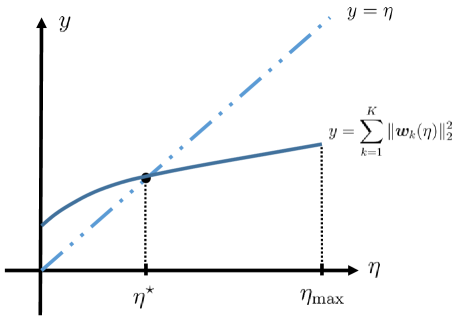
Figure 3: Illustration of Proposition 3. It is assumed that (P1) is feasible.

We first have the following proposition.

Proposition 2

Suppose that (P1) is feasible. Let $\{{\bm{w}}_{k}^{\star}\}$ be the optimal DL beamformers of (P1) and let $\eta^{\star}\triangleq\sum_{k=1}^{K}\|{\bm{w}}_{k}^{\star}\|_{2}^{2}$. Then
(a) $\eta^{\star}$ is unique;
(b) When $\eta=\eta^{\star}$, $\{{\bm{w}}_{k}(\eta)\}$ of (P_η) is optimal to (P1) and satisfies $\sum_{k=1}^{K}\|{\bm{w}}_{k}(\eta)\|_{2}^{2}=\eta^{\star}$;
(c) $F(\eta)$ of (P_η) is monotonically increasing with $\eta$.

Proof: See Appendix B. $\blacksquare$

Proposition 2 suggests that one can solve (P1) by searching the unique optimal $\eta^{\star}$ of (P_η). The following result provides important insight into how $\eta$ can be searched efficiently.

Proposition 3

Suppose that (P1) is feasible and that (P_η) is feasible for $\eta\in[0,\eta_{\max}]$, where $\eta_{\max}>0$. Then
(a) $\sum_{k=1}^{K}\|{\bm{w}}_{k}(\eta)\|_{2}^{2}$ of (P_η) is concave and increasing with respect to $\eta\in[0,\eta_{\max}]$.
(b) $\sum_{k=1}^{K}\|{\bm{w}}_{k}(\eta)\|_{2}^{2}>\eta$ if and only if $\eta<\eta^{\star}$.
Moreover, (P1) is infeasible if and only if (P_η) has $\sum_{k=1}^{K}\|{\bm{w}}_{k}(\eta)\|_{2}^{2}>\eta$ for all $\eta\in[0,\eta_{\max}]$.

Proof: See Appendix C. $\blacksquare$

From Proposition 3, we can visualize the function $\sum_{k=1}^{K}\|{\bm{w}}_{k}(\eta)\|_{2}^{2}$ as in Figure 3, provided that (P1) is feasible. Therefore, one can search the optimal $\eta^{\star}$ in a bisection fashion, by comparing the values of $\sum_{k=1}^{K}\|{\bm{w}}_{k}(\eta)\|_{2}^{2}$ and $\eta$. Specifically, if $\sum_{k=1}^{K}\|{\bm{w}}_{k}(\eta)\|_{2}^{2}>\eta$, $\eta$ should be increased, whereas if $\sum_{k=1}^{K}\|{\bm{w}}_{k}(\eta)\|_{2}^{2}\leq\eta$, then $\eta$ should be decreased. Moreover, if it happens that $\sum_{k=1}^{K}\|{\bm{w}}_{k}(\eta)\|_{2}^{2}>\eta$ for all $\eta\in[0,P_{\max}]$, where $P_{\max}$ denotes some bisection upper bound, then it will make $\eta$ converges to the bisection upper bound and thus one can declare that (P1) is infeasible for $\sum_{k=1}^{K}\|{\bm{w}}_{k}\|_{2}^{2}\leq P_{\max}$. Based on these observations, we develop a bisection method for solving (P1) in Algorithm 1. In Algorithm 1, the parameter $P_{\max}$ denotes the bisection upper bound and is the maximum DL transmission power budget.

Algorithm 1 Proposed bisection algorithm for solving (P1).

1:  Set $\eta^{\ell b}=0$ and $\eta^{ub}=P_{\max}$.

2:  repeat

3:     Set $\eta^{m}\leftarrow\frac{\eta^{ub}+\eta^{\ell b}}{2}.$

4:     Solve (P_η) by solving (29) and (30) in order.

5:     If (P_η) is infeasible or if (P_η) is feasible and $\sum_{k=1}^{K}\|{\bm{w}}_{k}(\eta^{m})\|_{2}^{2}\leq\eta^{m}$, set $\eta^{ub}\leftarrow\eta^{m}$; otherwise set $\eta^{\ell b}\leftarrow\eta^{m}$.

6:  until $|\eta^{ub}-\eta^{\ell b}|\leq\epsilon$, where $\epsilon$ is a preset value. If $|\eta^{ub}-P_{\max}|\leq\epsilon$, then declare that (P1) is infeasible.

Since both the bisection algorithm and the subproblems (29) and (30) have polynomial-time complexity, (P1) is polynomial-time solvable.

Theorem 1

Suppose that (P1) is feasible. Then Algorithm 1 globally solves (P1) in polynomial time.

From the proof of Proposition 3(a), it is worth noting that not only $\sum_{k=1}^{K}\|{\bm{w}}_{k}(\eta)\|_{2}^{2}$ but also $\sum_{\ell=1}^{L}p_{\ell}^{\rm U}(\eta)$ are concave functions of $\eta$. When applying this insight to the original problem (P), it implies that the objective function $\sum_{k=1}^{K}\|{\bm{w}}_{k}\|_{2}^{2}+\sum_{\ell=1}^{L}p_{\ell}^{\rm U}$ is concave function of the SI power. Therefore, for such minimization problem, it is unlikely to solve (P) jointly with respect to all the variables $\{{\bm{w}}_{k},{\bm{v}}_{\ell},p_{\ell}^{\rm U}\}$ in a convex manner. In light of this, we resort to approximation methods in the next section.

IV KKT Solutions to (P) via Alternating Optimization

In this section, we consider the general design problem (P) in (20) and propose a suboptimal method to handle (P) by alternating optimization. In the first subsection, we present the proposed AO algorithm and show that the algorithm is guaranteed to converge to a Karush-Kuhn-Tucker (KKT) point of (P). In the second subsection, we generalize the UDD in HD systems [27, 25] to the FD system and use it to develop a computationally efficient fixed-point based AO algorithm.

IV-A Proposed AO Algorithm

The proposed AO algorithm shares a similar strategy as the iterative algorithms proposed in [28, 29, 30] for joint transmit and receive beamforming optimization in HD MIMO systems. For the considered problem (P), we observe that, when the UL beamformer $\{{\bm{v}}_{\ell}\}$ are fixed, (P) can be recast as a convex SOCP, through simple change of variables. Moreover, when the DL beamformer $\{{\bm{w}}_{k}\}$ and UL power $\{p_{\ell}^{\rm U}\}$ are fixed, $\{{\bm{v}}_{\ell}\}$ has a simple closed-form expression.

Specifically, let us assume that the UL beamforming vectors $\{{\bm{v}}_{\ell}\}$ are fixed in (P). We have

$$\min_{\begin{subarray}{c}\{{\bm{w}}_{k}\},\{p_{\ell}^{\rm U}\geq 0\}\end{subarray}}~{}\sum_{k=1}^{K}\|{\bm{w}}_{k}\|_{2}^{2}+\sum_{\ell=1}^{L}p_{\ell}^{\rm U}$$ (33a)

$${\rm s.t.}~{}~{}\frac{|{\bm{h}}_{i}^{H}{\bm{w}}_{i}|^{2}/{\rho_{i}^{\rm D}}}{\sum_{k=1}^{K}{\bm{w}}_{k}^{H}\tilde{}{\bm{H}}_{i}{\bm{w}}_{k}+\hat{\sigma}_{i}^{2}({\bm{p}}^{\rm U})}\geq 1,~{}\forall i\in{\mathcal{K}},$$ (33b)

$$~{}~{}\frac{p_{\ell}^{\rm U}|{\bm{v}}_{\ell}^{H}{\bm{g}}_{\ell}|^{2}/\rho_{\ell}^{\rm U}}{\sum_{j=1}^{L}p_{j}^{\rm U}{\bm{v}}_{\ell}^{H}\tilde{}{\bm{G}}_{j}{\bm{v}}_{\ell}+\sum_{k=1}^{K}{\bm{w}}_{k}^{H}{\bf\Lambda}({\bm{v}}_{\ell},{\bm{R}}_{{\bf\Phi}_{0}}){\bm{w}}_{k}+\tilde{\sigma}_{z}^{2}}\geq 1,~{}\forall\ell\in{\mathcal{L}},$$ (33c)

$$~{}~{}{\rm ADC}({\bm{W}},{\bm{p}}^{\rm U})\preceq\gamma^{\rm ADC}{\bm{I}}_{N_{t}}.$$ (33d)

Note from (19) that (33d) are convex constraints. Besides, if $\{{\bm{w}}_{k}^{\star}\}$ is an optimal solution to (33), then any phase rotated version of $\{{\bm{w}}_{k}^{\star}\}$ is still an optimal solution. Let us consider in (33) the change of variables $q_{\ell}=\sqrt{p_{\ell}^{\rm U}}$, $\ell\in{\mathcal{L}}$, and apply proper phase rotation to $\{{\bm{w}}_{k}\}$ so that ${\bm{h}}_{k}^{H}{\bm{w}}_{k}$ is real-valued for all $k\in{\mathcal{K}}$. Then one can equivalently write (33) as follows

$$\min_{\begin{subarray}{c}\{{\bm{w}}_{k}\},\{q_{\ell}\geq 0\}\end{subarray}}~{}\sum_{k=1}^{K}\|{\bm{w}}_{k}\|^{2}+\sum_{\ell=1}^{L}q_{\ell}^{2}$$ (34a)

$${\rm s.t.}~{}~{}\frac{{\bm{h}}_{i}^{H}{\bm{w}}_{i}}{\sqrt{\rho_{i}^{\rm D}}}\geq\sqrt{\sum_{k=1}^{K}\|\tilde{}{\bm{H}}_{i}^{\frac{1}{2}}{\bm{w}}_{k}\|_{2}^{2}+\sum_{j=1}^{L}q_{j}^{2}|f_{ji}|^{2}+\sigma_{i}^{2}},~{}k\in{\mathcal{K}},$$ (34b)

$$\frac{q_{\ell}|{\bm{v}}_{\ell}^{H}{\bm{g}}_{\ell}|}{\sqrt{\rho^{\rm U}_{\ell}}}\geq\sqrt{\sum_{j=1}^{L}q_{j}^{2}{\bm{v}}_{\ell}^{H}\tilde{}{\bm{G}}_{j}{\bm{v}}_{\ell}+\sum_{k=1}^{K}\|{\bf\Lambda}^{\frac{1}{2}}({\bm{v}}_{\ell},{\bm{R}}_{{\bf\Phi}_{0}}){\bm{w}}_{k}\|_{2}^{2}+\tilde{\sigma}_{z}^{2}},~{}\forall\ell\in{\mathcal{L}},$$ (34c)

$${\rm ADC}({\bm{W}},{\bm{p}}^{\rm U})\preceq\gamma^{\rm ADC}{\bm{I}}_{N_{t}}.$$ (34d)

​​Problem (34) is an SOCP which can be solved by standard convex solvers.

On the other hand, suppose that $\{{\bm{w}}_{k}\}$ and $\{p_{\ell}^{\rm U}\}$s are fixed in (P). Then the optimal ${\bm{v}}_{\ell}$ that maximizes ${\rm SINR}_{\ell}^{\rm U}$ in (20c) (i.e., (16)) is the maximum SINR beamformer

$${\bm{v}}_{\ell}=\frac{{\bf M}_{\ell}^{-1}{\bm{g}}_{\ell}}{\|{\bf M}_{\ell}^{-1}{\bm{g}}_{\ell}\|_{2}},$$ (35)

where ${\bf M}_{\ell}\triangleq\sum_{j=1}^{L}p_{j}^{\rm U}\tilde{}{\bm{G}}_{j}+{\bm{\Omega}}({\bm{W}},{\bm{R}}_{{\bf\Phi}_{0}})+\tilde{\sigma}_{z}^{2}{\bm{I}}_{N_{t}}.$

As a result, we propose to handle (P) via updating $(\{{\bm{w}}_{k}\},\{p_{\ell}^{\rm U}\})$ by solving (34) and updating $\{{\bm{v}}_{\ell}\}$ by (35) in an alternating fashion, as shown in Algorithm 2. If given the initial beamforming vectors $\{{\bm{v}}_{\ell}^{(0)}\}$, problem (34) (i.e., (33)) is infeasible, then the algorithm shall declare infeasibility. However, this does not necessarily imply that (P) is infeasible. When (33) is feasible given the initial $\{{\bm{v}}_{\ell}^{(0)}\}$, one can show that the AO algorithm converges to a KKT solution of (P).

Algorithm 2 Proposed SOCP-based AO algorithm for solving (P) in (20).

1:  Given initial UL beamforming vectors ${\bm{v}}_{\ell}^{(0)}$, $\ell=1,\ldots,L$; set $t\leftarrow 0.$ Declare infeasibility if (34) is infeasible given $\{{\bm{v}}_{\ell}^{(0)}\}$.

2:  repeat

3:     Given $\{{\bm{v}}_{\ell}^{(t)}\}$, obtain $(\{{\bm{w}}_{k}^{(t+1)}\},\{(p_{\ell}^{\rm U})^{(t+1)}\})$ by solving (34) (i.e., the SOCP reformulation of (33)).

4:     Given $(\{{\bm{w}}_{k}^{(t+1)}\},\{(p_{\ell}^{\rm U})^{(t+1)}\})$, obtain $\{{\bm{v}}_{\ell}^{(t+1)}\}$ by (35).

5:     $t\leftarrow t+1.$

6:  until a predefined convergence condition is satisfied.

Theorem 2

Suppose that (33) is feasible given initial ${\bm{v}}_{\ell}^{(0)}$, $\ell\in{\mathcal{L}}$. For Algorithm 2, the total power $\sum_{k=1}^{K}\|{\bm{w}}_{k}^{(t)}\|_{2}^{2}+\sum_{\ell=1}^{L}(p_{\ell}^{\rm U})^{(t)}$ is non-increasing with the iteration number $t$ and converges as $t\to\infty.$ Moreover, any limit point of $(\{{\bm{w}}_{k}^{(t+1)}\},\{(p_{\ell}^{\rm U})^{(t+1)}\},\{{\bm{v}}_{\ell}^{(t+1)}\})$ is a KKT point of (P).

Proof: It is easy to show that the objective value $\sum_{k=1}^{K}\|{\bm{w}}_{k}^{(t)}\|_{2}^{2}+\sum_{\ell=1}^{L}(p_{\ell}^{\rm U})^{(t)}$ is non-increasing. The proof of $(\{{\bm{w}}_{k}^{(t+1)}\},\{(p_{\ell}^{\rm U})^{(t+1)}\},\{{\bm{v}}_{\ell}^{(t+1)}\})$ converging to a KKT point of problem (P) can follow [31, Section IV]. Firstly, analogous to [31, Lemma 4] and using (34), one can show that problem (33) has a unique solution up to a phase rotation to $\{{\bm{w}}_{k}\}.$ Then, following a similar argument as in [31, Proposition 1], one can prove that any limit point of $(\{{\bm{w}}_{k}^{(t+1)}\},\{(p_{\ell}^{\rm U})^{(t+1)}\},\{{\bm{v}}_{\ell}^{(t+1)}\})$ is a KKT point of (P). The details are omitted here. $\blacksquare$

IV-B FD UDD and Fixed Point Method for Solving (33)

In this subsection, we show that the FD problem (33) has a duality property that resembles the UDD (i.e., Lemma 3) in HD systems. Moreover, similar to the fixed-point method for solving the HD problems [22, 19], the FD problem (33) can also be solved by efficient fixed-point iterations. To illustrate these methods, let us consider a partial Lagrange dual problem of (33)

$$\max_{{\bm{\nu}}\succeq{\bm{0}}}~{}\psi({\bm{\nu}})+(\sigma_{z}^{2}-\gamma^{\rm ADC}){\bf 1}^{T}{\bm{\nu}}$$ (36)

where $\psi({\bm{\nu}})$ is given by

$${\sf(P2)}~{}~{}\psi({\bm{\nu}})=\min_{\begin{subarray}{c}\{{\bm{w}}_{k}\},\{p_{\ell}^{\rm U}\geq 0\}\end{subarray}}~{} \sum_{k=1}^{K}{\bm{w}}_{k}^{H}{\bm{B}}{\bm{w}}_{k}+\sum_{\ell=1}^{L}p_{\ell}^{\rm U}b_{\ell}$$ (37a)

$${\rm s.t.}~{}~{} \eqref{eqn: prob formulation AO_cons1},~{}\eqref{eqn: prob formulation AO_cons2}.$$ (37b)

Here, ${\bm{\nu}}=[\nu_{1},\ldots,\nu_{N_{t}}]^{T}\in\mathbb{R}^{N_{t}}$ contain the dual variables associated with the ADC input power constraint (33d); for notational simplicity, it is also defined that ${\bm{B}}\triangleq{\bm{I}}_{N_{t}}+\sum_{n=1}^{N_{t}}\nu_{n}{\bm{\Upsilon}}_{n}(\{{\bm{R}}_{\Phi_{0},m}\})$ and $b_{\ell}\triangleq 1+\sum_{n=1}^{N_{t}}\nu_{n}|{\bm{e}}_{n}^{T}{\bm{g}}_{j}|^{2}$ for all $\ell\in{\mathcal{L}}.$ Owing to the hidden convexity of problem (33) (i.e., (34)), one can show that problem (33) in fact has a zero duality gap (see, e.g., [32, Proposition 1]). Therefore, solving the dual problem (36) is equivalent to solving problem (33). As a standard approach, one can solve problem (36) by the subgradient method [33]. In each update of the subgradient method, one has to solve the subproblem (P2).

The following proposition shows that (P2) has an equivalent duality problem:

Proposition 4

Suppose that problem (P2) in (37) is feasible. Then (P2) achieves the same optimal objective value as the following problem

$$(\{\tilde{}{\bm{w}}_{k}^{\star}\},{\bm{\lambda}}^{\star},{\bm{\mu}}^{\star})=\arg\min_{\begin{subarray}{c}\{\tilde{}{\bm{w}}_{k}\},{\bm{\lambda}},{\bm{\mu}}\succeq{\bm{0}}\end{subarray}}~{}{\bm{\lambda}}^{T}{\bm{\sigma}}^{2}+\tilde{\sigma}_{z}^{2}{\bm{\mu}}^{T}{\bf 1}$$ (38a)

$${\rm s.t.}~{}~{}\frac{\lambda_{k}|\tilde{}{\bm{w}}_{k}^{H}{\bm{h}}_{k}|^{2}/\rho_{k}^{\rm D}}{\tilde{}{\bm{w}}_{k}^{H}{\bm{Q}}({\bm{\lambda}},{\bm{\mu}})\tilde{}{\bm{w}}_{k}}\geq 1,~{}k\in{\mathcal{K}},$$ (38b)

$$~{}~{}~{}~{}~{}\frac{\mu_{\ell}|{\bm{v}}_{\ell}^{H}{\bm{g}}_{\ell}|^{2}/\rho_{\ell}^{\rm U}}{\sum_{j=1}^{L}\mu_{j}{\bm{v}}_{\ell}^{H}\tilde{}{\bm{G}}_{j}{\bm{v}}_{\ell}+\sum_{k=1}^{K}\lambda_{k}|f_{\ell k}|^{2}+b_{\ell}}\geq 1,\ell\in{\mathcal{L}},$$ (38c)

$$~{}~{}~{}~{}~{}\|\tilde{}{\bm{w}}_{k}\|_{2}=1,~{}k\in{\mathcal{K}},$$ (38d)

where ${\bm{\sigma}}^{2}\triangleq[\sigma_{1}^{2},\ldots,\sigma_{K}^{2}]^{T}$ and ${\bm{Q}}({\bm{\lambda}},{\bm{\mu}})\triangleq\sum_{i=1}^{K}\lambda_{i}\tilde{}{\bm{H}}_{i}+\sum_{\ell=1}^{L}\mu_{\ell}{\bf\Lambda}({\bm{v}}_{\ell},{\bm{R}}_{{\bf\Phi}_{0}})+{\bm{B}}.$ Moreover, the optimal beamforming direction of (P2) can be obtained via (38) as

$$\frac{{\bm{w}}_{k}^{\star}}{\|{\bm{w}}_{k}^{\star}\|_{2}}=\tilde{}{\bm{w}}_{k}^{\star}=\frac{{\bm{Q}}^{-1}({\bm{\lambda}}^{\star},{\bm{\mu}}^{\star}){\bm{h}}_{k}}{\|{\bm{Q}}^{-1}({\bm{\lambda}}^{\star},{\bm{\mu}}^{\star}){\bm{h}}_{k}\|_{2}},~{}k\in{\mathcal{K}},$$ (39)

where $\{{\bm{w}}_{k}^{\star}\}$ denotes the optimal $\{{\bm{w}}_{k}\}$ of (P2).

Proof: See Appendix D. $\blacksquare$

By comparing (38b) and (38c) with (33b) and (33c), respectively, one can see that problem (38) can be regarded as a weighted power minimization problem for a virtual FD system with $K$ UMUs and $L$ DMUs. In particular, $\{\mu_{\ell}\}$ and $\{\lambda_{k}\}$ are the DL and UL powers in the virtual FD system, respectively, and all the variables and channels originally associated with the DL (resp. UL) are now associated with UL (resp. DL) in the virtual system.

Analogous to the HD UDD which is used to develop a fixed-point method [22, 19], we use the above FD UDD to develop a new fixed-point method to solve (P2). To see this, notice that (38b) and (38c) must hold with equality at the optimum. By substituting (39) into them, constraints (38b) and (38c) can be equivalently written as

$$\lambda_{k}=\mathcal{F}_{k}^{\rm U}({\bm{\lambda}},{\bm{\mu}})\triangleq\frac{1}{{\bm{h}}_{k}^{H}{\bm{Q}}^{-1}({\bm{\lambda}},{\bm{\mu}}){\bm{h}}_{k}/\rho_{{k}}^{\rm D}},~{}\forall k\in{\mathcal{K}},$$ (40)

$$\mu_{\ell}=\mathcal{F}_{\ell}^{\rm D}({\bm{\lambda}},{\bm{\mu}})\triangleq\frac{\sum_{j=1}^{L}\mu_{j}{\bm{v}}_{\ell}^{H}\tilde{}{\bm{G}}_{j}{\bm{v}}_{\ell}+\sum_{k=1}^{K}\lambda_{k}|f_{\ell k}|^{2}+b_{\ell}}{|\tilde{}{\bm{v}}_{\ell}^{H}{\bm{g}}_{\ell}|^{2}/\rho_{{\ell}}^{\rm U}},$$

$$~{}~{}~{}~{}~{}~{}~{}~{}~{}~{}~{}~{}~{}~{}~{}~{}~{}~{}~{}~{}~{}~{}~{}~{}~{}~{}~{}~{}~{}~{}~{}~{}~{}~{}~{}~{}~{}~{}~{}~{}~{}~{}~{}~{}~{}~{}~{}~{}~{}~{}~{}~{}~{}\forall\ell\in{\mathcal{L}}.$$ (41)

By defining

$${\bm{\mathcal{F}}}({\bm{\lambda}},{\bm{\mu}})\triangleq[\mathcal{F}_{1}^{\rm U}({\bm{\lambda}},{\bm{\mu}}),\ldots,\mathcal{F}_{K}^{\rm U}({\bm{\lambda}},{\bm{\mu}}),$$

$$~{}~{}~{}~{}~{}~{}~{}~{}~{}~{}~{}~{}~{}~{}~{}~{}~{}~{}~{}~{}\mathcal{F}_{1}^{\rm D}({\bm{\lambda}},{\bm{\mu}}),\ldots,\mathcal{F}_{L}^{\rm D}({\bm{\lambda}},{\bm{\mu}})]^{T},$$

we obtain the following fixed point equation

$$[{\bm{\lambda}}^{T}{\bm{\mu}}^{T}]^{T}={\bm{\mathcal{F}}}({\bm{\lambda}},{\bm{\mu}}).$$ (42)

Lemma 4

Suppose that problem ${\sf(P2)}$ in (37) is feasible. Then the optimal solution $({\bm{\lambda}}^{\star},{\bm{\mu}}^{\star})$ of (38) is the unique fixed point of (42). Moreover, given any initial $({\bm{\lambda}}^{(0)},{\bm{\mu}}^{(0)})$, $({\bm{\lambda}}^{\star},{\bm{\mu}}^{\star})$ can be achieved by the following fixed-point iterations

$$[({\bm{\lambda}}^{(t+1)})^{T}({\bm{\mu}}^{(t+1)})^{T}]^{T}\leftarrow{\bm{\mathcal{F}}}({\bm{\lambda}}^{(t)},{\bm{\mu}}^{(t)})$$ (43)

as $t\to\infty$.

Proof: As shown in (42), once (P2) is feasible, $({\bm{\lambda}}^{\star},{\bm{\mu}}^{\star})$ is a fixed point. So the fixed point exists for (42). To show that $({\bm{\lambda}}^{\star},{\bm{\mu}}^{\star})$ is the unique fixed point and the fixed-point iterations in (43) converges to $({\bm{\lambda}}^{\star},{\bm{\mu}}^{\star})$ for arbitrary $({\bm{\lambda}}^{(0)},{\bm{\mu}}^{(0)})$, it suffices to show that ${\bm{\mathcal{F}}}$ is a standard interference function [34, Theorem 2]; that is, each $\mathcal{F}_{k}^{\rm U}$ and $\mathcal{F}_{\ell}^{\rm D}$ should satisfy positivity, monotonicity and scalability properties, for all $k\in{\mathcal{K}}$ and $\ell\in{\mathcal{L}}.$ The part of $\mathcal{F}_{k}^{\rm U}$ can be proved following exactly the same arguments as in [19, Appendix II], while the part of $\mathcal{F}_{\ell}^{\rm D}$ is easy to verity to be true. The details are omitted. $\blacksquare$

Once $({\bm{\lambda}}^{\star},{\bm{\mu}}^{\star})$ is obtained by the above fixed-point iterations, the optimal DL beamforming direction $\{\tilde{}{\bm{w}}_{k}^{\star}\}$ can be obtained by (39). What remains for solving (P2) is to obtain the optimal DL transmission powers $\{p_{k}^{\rm D\star}\}$ and UL transmission power $\{p_{\ell}^{\rm U\star}\}$. To show how they can be obtained, let us first introduce some notations. Let ${\bm{S}}_{11}$ be a $K\times K$ matrix whose $k$th diagonal entry is $|{\bm{h}}_{k}^{H}\tilde{}{\bm{w}}_{k}^{\star}|^{2}/\rho_{k}^{\rm D}-(\tilde{}{\bm{w}}^{\star}_{k})^{H}\tilde{}{\bm{H}}_{k}\tilde{}{\bm{w}}^{\star}_{k}$ and $(k,i)$th off-diagonal entry is $-(\tilde{}{\bm{w}}^{\star}_{i})^{H}\tilde{}{\bm{H}}_{k}\tilde{}{\bm{w}}^{\star}_{i}$. Moreover, define ${\bm{S}}_{12}$ as a $K\times L$ matrix with the $(k,\ell)$th entry being $-|f_{\ell k}|^{2}$. Similarly, let us define an $L\times L$ matrix ${\bm{S}}_{22}$ which has the $\ell$th diagonal entry being $|{\bm{v}}_{\ell}^{H}{\bm{g}}_{\ell}|^{2}/\rho^{\rm U}_{\ell}-{\bm{v}}_{\ell}^{H}\tilde{}{\bm{G}}_{\ell}{\bm{v}}_{\ell}$ and the $(k,i)$th off-diagonal entry being $-{\bm{v}}_{\ell}^{H}\tilde{}{\bm{G}}_{j}{\bm{v}}_{\ell}$. Lastly, define an $L\times K$ matrix ${\bm{S}}_{21}$ whose $(\ell,k)$th entry is $-\tilde{}{\bm{w}}_{k}^{H}{\bf\Lambda}({\bm{v}}_{\ell},{\bm{R}}_{{\bf\Phi}_{0}})\tilde{}{\bm{w}}_{k}$. Then, given $\{{\bm{w}}_{k}^{\star}\}$, constraints (33b) and (33c) can be compactly expressed as

$${\bm{S}}(\{\tilde{}{\bm{w}}_{k}^{\star}\},\{{\bm{v}}_{\ell}\})\begin{bmatrix}{\bm{p}}^{\rm D}\\ {\bm{p}}^{\rm U}\end{bmatrix}\succeq\begin{bmatrix}{\bm{\sigma}}^{2}\\ \tilde{\sigma}_{z}^{2}{\bf 1}\end{bmatrix},$$ (44)

where ${\bm{p}}^{\rm D}=[p_{1}^{\rm D},\ldots,p_{K}^{\rm D}]^{T}$ and

$${\bm{S}}(\{\tilde{}{\bm{w}}_{k}^{\star}\},\{{\bm{v}}_{\ell}\})=\begin{bmatrix}{\bm{S}}_{11}&{\bm{S}}_{12}\\ {\bm{S}}_{21}&{\bm{S}}_{22}\end{bmatrix}.$$ (45)

The following lemma gives the closed-form solution of optimal power $(\{p_{k}^{\rm D\star}\},\{p_{\ell}^{\rm U\star}\})$.

Lemma 5

Suppose that problem (P2) in (37) is feasible, and that the optimal DL beamforming directions $\{\tilde{}{\bm{w}}_{k}^{\star}\}$ are given. Then the optimal DL and UL powers ${\bm{p}}^{\rm D\star}$ and ${\bm{p}}^{\rm U\star}$ are uniquely given by

$$\begin{bmatrix}{\bm{p}}^{\rm D\star}\\ {\bm{p}}^{\rm U\star}\end{bmatrix}={\bm{S}}^{-1}(\{\tilde{}{\bm{w}}_{k}^{\star}\},\{{\bm{v}}_{\ell}\})\begin{bmatrix}{\bm{\sigma}}^{2}\\ \tilde{\sigma}_{z}^{2}{\bf 1}\end{bmatrix}\succ{\bm{0}}.$$ (46)

Proof: Given that (P2) is feasible, constraints (33b) and (33c) will hold with equality at the optimum and ${\bm{p}}^{\rm D\star}$ and ${\bm{p}}^{\rm U\star}$ will be a solution to the linear system (44). To show that ${\bm{p}}^{\rm D\star}$ and ${\bm{p}}^{\rm U\star}$ are the unique solution, one can follow a similar arguments as in [25, Lemma 1]. A sufficient and necessary condition for the proof to be valid is that the diagonal elements of ${\bm{S}}_{11}$ and ${\bm{S}}_{22}$ have to be positive, i.e., $|{\bm{h}}_{k}^{H}\tilde{}{\bm{w}}_{k}^{\star}|^{2}/\rho_{k}^{\rm D}-(\tilde{}{\bm{w}}^{\star}_{k})^{H}\tilde{}{\bm{H}}_{k}\tilde{}{\bm{w}}^{\star}_{k}>0$ for all $k\in{\mathcal{K}}$ and $|{\bm{v}}_{\ell}^{H}{\bm{g}}_{\ell}|^{2}/\rho^{\rm U}_{\ell}-{\bm{v}}_{\ell}^{H}\tilde{}{\bm{G}}_{\ell}{\bm{v}}_{\ell}>0$ for all $\ell\in{\mathcal{L}}$. Recall from Proposition 4 that the optimal DL beamforming direction $\{{\bm{w}}_{k}^{\star}\}$ must satisfy (38b), i.e.,

$$\lambda_{k}^{\star}|{\bm{h}}_{k}^{H}\tilde{}{\bm{w}}_{k}^{\star}|^{2}/\rho_{k}^{\rm D}-(\tilde{}{\bm{w}}_{k}^{\star})^{H}(\lambda_{k}^{\star}\tilde{}{\bm{H}}_{k})\tilde{}{\bm{w}}_{k}^{\star}$$

$$-{({\bm{w}}_{k}^{\star})^{H}\bigg{(}\sum_{i\neq k}^{K}\lambda_{i}^{\star}\tilde{}{\bm{H}}_{i}+\sum_{\ell=1}^{L}\mu_{\ell}^{\star}{\bf\Lambda}({\bm{v}}_{\ell},{\bm{R}}_{{\bf\Phi}_{0}})+{\bm{B}}\bigg{)}\tilde{}{\bm{w}}_{k}^{\star}}\geq 0.$$

Since $\sum_{i\neq k}^{K}\lambda_{i}^{\star}\tilde{}{\bm{H}}_{i}+\sum_{\ell=1}^{L}\mu_{\ell}^{\star}{\bf\Lambda}({\bm{v}}_{\ell},{\bm{R}}_{{\bf\Phi}_{0}})+{\bm{B}}\succ{\bm{0}}$ (due to ${\bm{B}}\succ{\bm{0}}$), we have $|{\bm{h}}_{k}^{H}\tilde{}{\bm{w}}_{k}^{\star}|^{2}/\rho_{k}^{\rm D}-(\tilde{}{\bm{w}}^{\star}_{k})^{H}\tilde{}{\bm{H}}_{k}\tilde{}{\bm{w}}^{\star}_{k}>0$. Analogously, since $\{{\bm{v}}_{\ell}\}$ satisfies (38c) and $\sum_{j\neq\ell}^{L}\mu_{j}^{\star}{\bm{v}}_{\ell}^{H}\tilde{}{\bm{G}}_{j}{\bm{v}}_{\ell}+\sum_{k=1}^{K}\lambda_{k}^{\star}|f_{\ell k}|^{2}+b_{\ell}>0$, it is clear that $|{\bm{v}}_{\ell}^{H}{\bm{g}}_{\ell}|^{2}/\rho^{\rm U}_{\ell}-{\bm{v}}_{\ell}^{H}\tilde{}{\bm{G}}_{\ell}{\bm{v}}_{\ell}>0$. $\blacksquare$

It is worth noting that Proposition 4, Lemma 4 and Lemma 5 essentially generalize the existing UDD and fixed-point method in HD systems [22, 27, 25] to the FD system. As seen, this generalization enables an efficient way to solve (P2). By combing it with the subgradient method, we come up with a low-complexity algorithm to solve problem (33) (i.e., (36)), which is shown in Algorithm 3. In particular, step 3 to step 7 of Algorithm 3 are the fixed-point iterations to obtain $({\bm{\lambda}}^{\star},{\bm{\mu}}^{\star})$; step 8 and step 9 are based on (39) and Lemma 5; step 10 is the subgradient update for dealing with the ADC input power constraint (33d), where $s^{(r)}$ is the step size. Comparing to directly solving the SOCP (34) using a general purpose solver, the proposed fixed-point based algorithm in Algorithm 3 is computationally more efficient, and therefore improving the computational efficiency of Algorithm 2.

Algorithm 3 Proposed fixed-point based algorithm for solving subproblem (33) in Algorithm 2.

1:  Given initial variables ${\bm{\nu}}^{(0)}={\bm{0}}$; set $r\leftarrow 0.$

2:  repeat

3:     set $t\leftarrow 0$ and initial ${\bm{\lambda}}^{(0)}={\bm{0}}$ and ${\bm{\mu}}^{(0)}={\bm{0}}.$

4:     repeat

5:        $[{\bm{u}}^{(t+1)}:=({\bm{\lambda}}^{(t+1)})^{T}({\bm{\mu}}^{(t+1)})^{T}]^{T}\leftarrow{\bm{\mathcal{F}}}({\bm{\lambda}}^{(t)},{\bm{\mu}}^{(t)})。$

6:        $t\leftarrow t+1$

7:     until $\|{\bm{u}}^{(t+1)}-{\bm{u}}^{(t)}\|_{2}/\|{\bm{u}}^{(t)}\|_{2}\leq\epsilon_{1}$. Denote the converged results as ${\bm{\lambda}}^{\star}$ and ${\bm{\mu}}^{\star}$.

8:     Obtain $\{\tilde{}{\bm{w}}_{k}^{\star}\}$ by (39), and obtain $\{(p_{k}^{\rm D\star})\}$ and $\{(p_{\ell}^{\rm U\star})\}$ by (46).

9:     ${\bm{w}}_{k}^{\star}\leftarrow\sqrt{(p_{k}^{\rm D\star})}\tilde{}{\bm{w}}_{k}^{\star},~{}\forall k\in{\mathcal{K}}.$

10:     ${\bm{\nu}}^{(r+1)}\leftarrow{\bm{\nu}}^{(r)}+s^{(r)}({\rm diag}({\rm ADC}({\bm{W}}^{\star},{\bm{p}}^{\rm U\star})-\gamma^{\rm ADC}{\bm{I}}_{N_{t}}))$.

11:     $r\leftarrow r+1.$

12:  until $\|{\bm{\nu}}^{(r+1)}-{\bm{\nu}}^{(r)}\|_{2}/\|{\bm{\nu}}^{(r)}\|_{2}\leq\epsilon_{2}$

V Simulation Results

In the simulation, we consider a wireless system as described in Section II-A and Figure 1. The FD BS has $10$ antennas ($N_{t}=10$) for simultaneous UL and DL communications [24, 8] . The channel coefficients $\{{\bm{h}}_{i}\}$,$\{{\bm{g}}_{j}\},$ $\{f_{ji}\}$ and ${\bm{H}}_{0}$ are composed by large-scale path loss as well as small scale Rayleigh fadings. In particular, the path loss between the MUs and the BS is set to $-80$ dB and that between the UMUs and DMUs is set to $-83$ dB. The SI channel has a $-10$ dB path loss [24, 8]. Besides, following [8], there is additional $-24$ dB cross-talk path loss for neighboring antennas and further $-6$ dB path loss for farther antennas. That is, the path loss between (transmit) antenna $i$ and (receive) antenna $j$ in the SI channel is -10dB for all $i=j$ and $-34-6|i-j-1|$ dB, for all $i\neq j$, where $i,j\in\{1,\ldots,N_{t}\}$. Define ${\bm{T}}$ (resp. ${\bm{C}}$) as an $N_{t}$ by $N_{t}$ Toeplitz matrix with the first row being $[1,10^{\frac{-24}{20}},10^{\frac{-30}{20}},\ldots,10^{\frac{-24-6(N_{t}-2)}{20}}]$ (resp. $[1,0.9,0.9^{2},\ldots,0.9^{N_{t}-1}$]). We model the correlation matrix of SI channel ${\bm{H}}_{0}$ as

$$\!\!\!\!\!{\bm{R}}_{{\bm{H}}_{0}} ={\mathbb{E}}[{\rm vec}({\bm{H}}_{0}){\rm vec}({\bm{H}}_{0})^{T}]$$

$$=\bigg{(}10^{\frac{-10}{10}}[{\rm vec}({\bm{T}}){\rm vec}({\bm{T}})^{T}]\bigg{)}\odot\bigg{(}{\bf 1}_{N_{t}\times N_{t}}\otimes{\bm{C}}\bigg{)},$$ (47)

where $\odot$ is the (element-wise) Hadamard product; $\otimes$ is the Kronecker product and ${\bf 1}_{N_{t}\times N_{t}}$ is the $N_{t}$ by $N_{t}$ all-one matrix. The first term in the RHS of (47) accounts for the cross-talk path loss, while the second term is for modeling the decreasing correlation between adjacent antennas. To model ${\bm{R}}_{{\bf\Phi}_{0}}$, we assume that the analog SIC scheme uses pilot-aided linear minimum mean squared error (LMMSE) channel estimation to estimate ${\bm{H}}_{0}$ [35]. Then, ${\bm{R}}_{{\bf\Phi}_{0}}$ is given by ${\bm{R}}_{{\bf\Phi}_{0}}={\bm{R}}_{{\bm{H}}_{0}}-{\bm{R}}_{{\bm{H}}_{0}}\big{(}{\bm{R}}_{{\bm{H}}_{0}}+\frac{\sigma_{z}^{2}}{E}{\bm{I}}_{N_{t}^{2}}\big{)}^{-1}{\bm{R}}_{{\bm{H}}_{0}},$ where $E>0$ denotes the energy of training signals. As seen, the larger $E$ is, the more powerful the analog SIC is. If not mentioned specifically, we set various parameters as follows: $\sigma_{z}^{2}=\sigma_{i}^{2}=-85$ dBm, $\beta_{1}=\beta_{2}=-30$ dB, $\delta_{1}=-50$ dB and $\delta_{2}=-20$ dB. For Algorithm 1, $P_{\max}$ is set to 40 dbm and $\epsilon$ is set to $10^{-3}$. Problems (29) and (30) are solved by the classical fixed-point method [22, 19]. For Algorithm 2, the stopping condition is set to the relative improvement of objective value of (P) being less than $10^{-6}$. Instead of using a convex solver to solve the SOCP (34), we use Algorithm 3 to solve problem (33) since they two yield the same performance theoretically. The parameters are set to $\epsilon_{1}=10^{-9}$, $\epsilon_{2}=10^{-3}$ and $s^{(r)}=1$ (constant step size). The initial $\{{\bm{v}}_{\ell}^{(0)}\}$ is set to the zero forcing (ZF) beamfomer, i.e., ${\bm{v}}_{\ell}^{(0)}={\bm{G}}^{{\dagger}}{\bm{e}}_{\ell}$, for all $\ell\in{\mathcal{L}}$, where ${\bm{G}}^{\dagger}$ is the pseudo inverse of ${\bm{G}}=[{\bm{g}}_{1},\ldots,{\bm{g}}_{L}]^{T}$. Note that if the AO algorithm runs only one iteration, then it is the same as the ZF based scheme in [17]. Besides, if not mentioned specifically, the ADC input power constraint (20d) is not considered in order to assess how the ADC input signal power varies with system parameters if unconstrained.

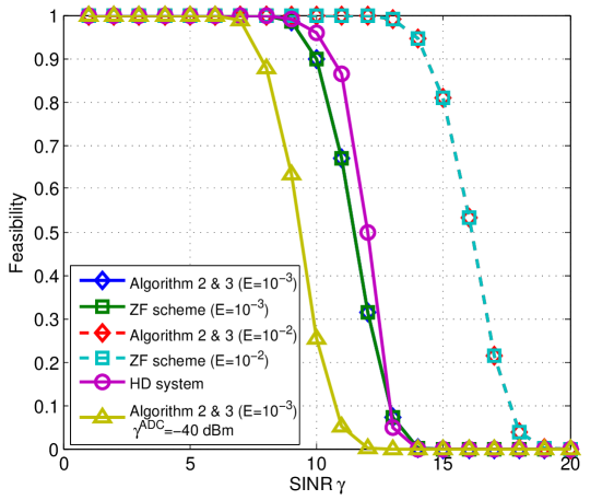
(a) Feasibility rate

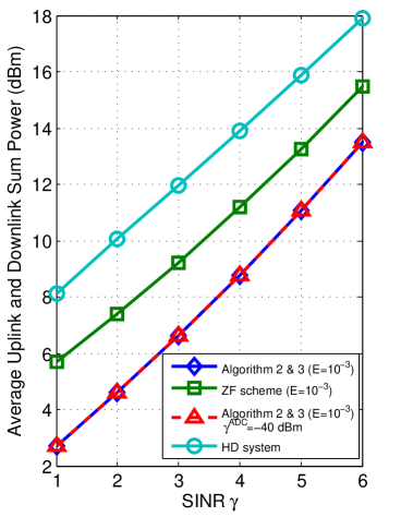
(b) Sum power

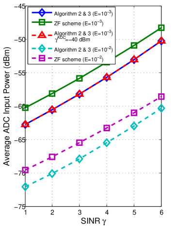
(c) ADC input signal power

Figure 4: Performance comparison of the proposed Algorithm 2 & 3 and the ZF scheme; $N_{t}=10$, $K=L=8$.

For simplicity, we let all UMUs and DMUs have the same SINR requirement, i.e., $\gamma\triangleq\gamma_{i}^{\rm D}=\gamma_{\ell}^{\rm U}$ for all $i\in{\mathcal{K}}$ and $\ell\in{\mathcal{L}}$. For a fair comparison, we set the SINR of MUs in the HD system as $\gamma_{\rm HD}\triangleq 2^{2\log_{2}(1+\gamma)}-1$. This implies that the information rate achieved by the HD MUs should be twice of that by the FD MUs [17]. All simulation results are obtained by averaging over 500 channel realizations.

Example 1: In Figure 4, we display the simulation results by comparing the proposed AO algorithm (i.e., Algorithm 2 and 3) with the ZF scheme and the HD system. The number of DMUs and UMUs are eight ($K=L=8$). First of all, one can observe from Figure 4(a) that the proposed AO algorithm has the same feasibility rate as the ZF scheme, which is expected, since the proposed AO algorithm is initialized by the ZF receive beamformer. However, one can see from Figure 4(b) and Figure 4(c) that the AO algorithm can yield about 3 dB lower sum power and ADC input power than the ZF scheme. It can also be seen from the two figures that for both $E=10^{-3}$ and $E=10^{-2}$, the FD system using the proposed AO algorithm is more power efficient than the HD system when both systems are feasible.

In Figure 4, we also present the performance of the proposed AO algorithm when the ADC input power constraint (20d) is imposed with $\gamma^{\rm ADC}=-40$ dBm. One can see from Figure 4(a) that the feasibility rate drops compared to that without the ADC input power constraint for $\gamma\geq 7$ dB. This implies that there exist realizations for which the ADC input signal power is higher than -40 dBm and this happens more frequently when $\gamma$ increases. Since from Figure 4(c) that the ADC input power is less than -40 dBm for $\gamma\leq 6$ dB, Figure 4(b) shows that the AO algorithm with the ADC input power constraint performs equally well as its counterpart without the ADC input power constraint in this regime.

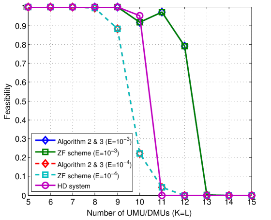
(a) Feasibility rate

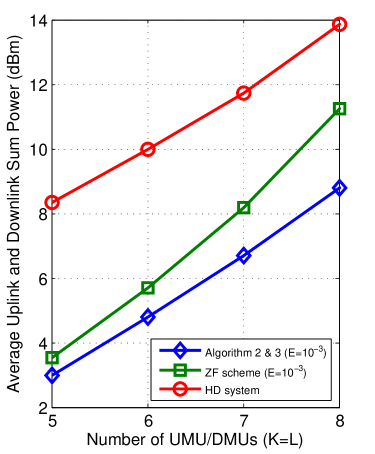
(b) Sum power

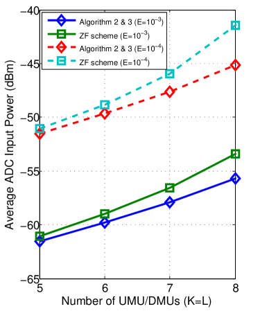
(c) ADC input signal power

Figure 5: Performance comparison of the proposed Algorithm 2 & 3 and the ZF scheme; $N_{t}=10$, $\gamma=5$ dB.

Example 2: In Figure 5, we present the results by considering various numbers of DMU/UMUs in the network. The SINR requirement is set to $\gamma=5$ dB. As expected, the system performance (feasibility rate and sum power) deteriorates when the number of MUs in the network increases. The ADC input power also increases since the SI power can increase both with the number of UMUs and the number of DMUs. One may notice that the feasibility rate of the proposed AO algorithm ($E=10^{-3}$) oscillates between $K=L=10$ and $K=L=11$. This is because the AO algorithm is initialized by different $\{{\bm{v}}_{\ell}^{(0)}\}$ when the number of UMUs changes. Finally, it can be observed from Figure 5(b) and Figure 5(c) that the more number of MUs in the network, the better the AO algorithm performs than the ZF scheme.

Example 3: In the last example, let us examine the performance of Algorithm 1 by assuming that the SI channel errors are i.i.d. Specifically, we let ${\bm{R}}_{{\bm{H}}_{0}}=\sigma_{{\bm{H}}_{0}}^{2}{\bm{I}}_{N_{t}^{2}}$ where $\sigma_{{\bm{H}}_{0}}^{2}=-10$ dB, and let $K=L=5$. The simulation results are presented in Figure 6. Firstly, one can observe from Figure 6(a) that there exists small discrepancy between the feasibility rates of the AO algorithm (Algorithm 2 and 3) and the bisection algorithm (Algorithm 1), especially when the feasibility rates are not 100%. We suspect that the AO algorithm actually achieves the same solution as the bisection algorithm under the simulation setting, and the discrepancy in the feasibility rate are caused by some numerical issues. This is evidenced by observing from Figure 6(b) and Figure 6(c) that the AO and bisection algorithms essentially yield the same sum power and ADC input power when both methods are feasible. Therefore, the simulation results imply that the AO algorithm may have achieved optimal or near-optimal solutions for the cases with ${\bm{R}}_{{\bm{H}}_{0}}=\sigma_{{\bm{H}}_{0}}^{2}{\bm{I}}_{N_{t}^{2}}$. From Figure 6(a), we again see that with the ADC input power constraint, the feasibility rates of the considered design problem decreases.

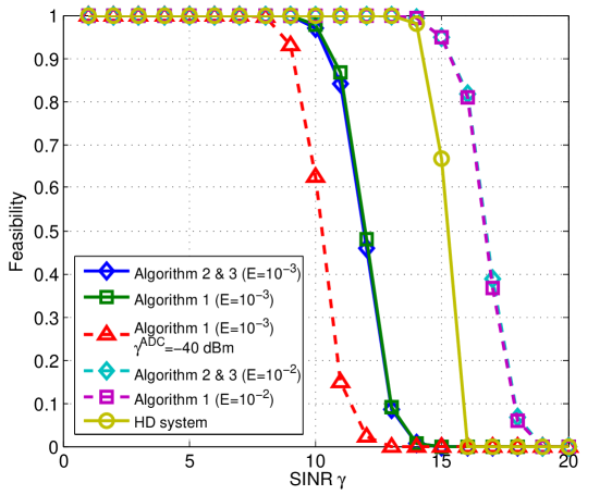
(a) Feasibility rate

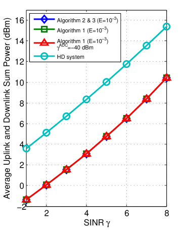
(b) Sum power

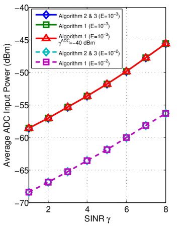
(c) ADC input signal power

Figure 6: Performance of the proposed Algorithm 1, 2 and 3; $N_{t}=10$, $K=L=5$, ${\bm{R}}_{\Phi_{0}}=\sigma_{\Phi_{0}}^{2}{\bm{I}}_{N_{t}^{2}}$ where $\sigma_{\Phi_{0}}^{2}=-10$ dB.

VI Conclusion

In this paper, by taking into account the non-ideal RF chains and analog/digital SIC, we have formulated the QoS-based linear transceiver design problem (P) which is not only constrained by the minimum SINR requirement of MUs but also by the maximum power at the ADC input. While such problem is non-convex and difficult to solve in general, we have shown that it can be solved to the global optimum when the SI channel estimation errors are i.i.d. Specifically, we have developed a bisection algorithm (Algorithm 1) that can achieve the global optimal solution in a polynomial-time complexity. To handle (P) in general, we have proposed a suboptimal AO algorithm (Algorithm 2). Moreover, we have generalized the UDD in the HD system to the FD system and proposed an efficient fixed-point based algorithm for solving (33) (Algorithm 3). The presented simulation results have shown that the proposed AO algorithm outperforms the ZF scheme. Moreover, when the SI channel estimation errors are i.i.d., the simulation results also suggest that the AO algorithm achieves a near-optimal solution. It is also observed that the FD system is more power efficient than the HD system especially when the QoS requirements are less stringent or when the number of MUs is moderate.

Appendix A Derivation of (12) and (13)

The derivation involves basic vector and matrix algebra. Note that we can write the first term of in the RHS of (II-A2) as

$$\delta_{1}{\bm{v}}^{H}_{\ell}{\mathbb{E}}[{\bf\Phi}_{0}{\bm{x}}(t){\bm{x}}^{H}(t){\bf\Phi}_{0}^{H}]{\bm{v}}_{\ell}$$

$$~{}~{}=\delta_{1}{\bm{v}}^{H}_{\ell}{\mathbb{E}}\bigg{[}{\bf\Phi}_{0}{\bm{W}}{\bm{W}}^{H}{\bf\Phi}_{0}^{H}\bigg{]}{\bm{v}}_{\ell}$$ (A.1)

$$~{}~{}=\delta_{1}\sum_{k=1}^{K}{\bm{w}}_{k}^{H}{\mathbb{E}}\bigg{[}{\bf\Phi}_{0}^{H}{\bm{v}}_{\ell}{\bm{v}}_{\ell}^{H}{\bf\Phi}_{0}\bigg{]}{\bm{w}}_{k}.$$ (A.2)

Besides, by (1), we can write the second term in the RHS of (II-A2) as

$$\delta_{2}{\bm{v}}_{\ell}^{H}{\mathbb{E}}[{\bf\Phi}_{0}{\bm{u}}_{\rm tx}[n]{\bm{u}}_{\rm tx}^{H}[n]{\bf\Phi}_{0}^{H}]{\bm{v}}_{\ell}$$

$$~{}~{}=(\delta_{2}\beta_{1}){\bm{v}}_{\ell}^{H}{\mathbb{E}}[{\bf\Phi}_{0}{\rm diag}({\bm{W}}{\bm{W}}^{H}){\bf\Phi}_{0}^{H}]{\bm{v}}_{\ell}$$ (A.3)

$$~{}~{}=(\delta_{2}\beta_{1})\sum_{k=1}^{K}\sum_{n=1}^{N_{t}}({\bm{v}}_{\ell}^{H}{\mathbb{E}}[{\bf\Phi}_{0}{\bm{e}}_{n}{\bm{e}}_{n}^{T}{\bf\Phi}_{0}^{H}]{\bm{v}}_{\ell})|w_{kn}|^{2}$$

$$~{}~{}=(\delta_{2}\beta_{1})\sum_{k=1}^{K}{\bm{w}}_{k}^{H}{\rm diag}\bigg{(}\{{\bm{v}}_{\ell}^{H}{\mathbb{E}}[{\bf\Phi}_{0}{\bm{e}}_{n}{\bm{e}}_{n}^{T}{\bf\Phi}_{0}^{H}]{\bm{v}}_{\ell}\}_{n}\bigg{)}{\bm{w}}_{k}.$$ (A.4)

Analogously, by (6) and (8), the third term in the RHS of (II-A2) can be written as

$$\delta_{2}{\bm{v}}_{\ell}^{H}{\mathbb{E}}[{\bm{u}}_{\rm rx}[n]{\bm{u}}_{\rm rx}^{H}[n]]{\bm{v}}_{\ell}$$

$$=(\delta_{2}\beta_{2}){\bm{v}}_{\ell}^{H}{\rm diag}\bigg{(}\sum_{j=1}^{L}{\bm{g}}_{j}{\bm{g}}_{j}^{H}p^{\rm U}_{j}+{\mathbb{E}}[{\bf\Phi}_{0}{\bm{W}}{\bm{W}}^{H}{\bf\Phi}_{0}^{H}]+\beta_{1}{\mathbb{E}}[{\bf\Phi}_{0}{\rm diag}({\bm{W}}{\bm{W}}^{H}){\bf\Phi}_{0}^{H}]+\sigma_{z}^{2}{\bm{I}}_{N_{t}}\bigg{)}{\bm{v}}_{\ell}$$

$$=(\delta_{2}\beta_{2}){\bm{v}}_{\ell}^{H}\bigg{(}\sum_{j=1}^{L}p^{\rm U}_{j}{\rm diag}(|{\bm{g}}_{j}|^{2})\bigg{)}{\bm{v}}_{\ell}+(\delta_{2}\beta_{2}){\bm{v}}_{\ell}^{H}{\rm diag}\bigg{(}{\mathbb{E}}[{\bf\Phi}_{0}{\bm{W}}{\bm{W}}^{H}{\bf\Phi}_{0}^{H}]$$

$$~{}~{}~{}~{}+\beta_{1}{\mathbb{E}}[{\bf\Phi}_{0}{\rm diag}({\bm{W}}{\bm{W}}^{H}){\bf\Phi}_{0}^{H}]+\sigma_{z}^{2}{\bm{I}}_{N_{t}}\bigg{)}{\bm{v}}_{\ell}$$ (A.5)

$$=(\delta_{2}\beta_{2})\bigg{[}{\bm{v}}_{\ell}^{H}\bigg{(}\sum_{j=1}^{L}p^{\rm U}_{j}{\rm diag}(|{\bm{g}}_{j}|^{2})\bigg{)}{\bm{v}}_{\ell}+\sum_{k=1}^{K}{\bm{w}}_{k}^{H}\bigg{(}\sum_{n=1}^{N_{t}}|v_{\ell,n}|^{2}{\mathbb{E}}\{{\bf\Phi}_{0}^{H}{\bm{e}}_{n}{\bm{e}}_{n}^{T}{\bf\Phi}_{0}\}\bigg{)}{\bm{w}}_{k}$$

$$+\beta_{1}\sum_{k=1}^{K}{\bm{w}}_{k}^{H}{\rm diag}\bigg{(}\!\!\bigg{\{}\!\!{\bm{v}}_{\ell}^{H}{\rm diag}\bigg{(}{\mathbb{E}}[{\bf\Phi}_{0}{\bm{e}}_{n}{\bm{e}}_{n}^{T}{\bf\Phi}_{0}^{H}]\bigg{)}{\bm{v}}_{\ell}\bigg{\}}_{n}\bigg{)}{\bm{w}}_{k}+\sigma_{z}^{2}\|{\bm{v}}_{\ell}\|_{2}^{2}\bigg{]}.$$ (A.6)

To simplify the notations, define

$${\bm{\Omega}}({\bm{W}},{\bm{R}}_{{\bf\Phi}_{0}})\triangleq\delta_{1}{\mathbb{E}}\bigg{[}{\bf\Phi}_{0}{\bm{W}}{\bm{W}}^{H}{\bf\Phi}_{0}^{H}\bigg{]}+(\delta_{2}\beta_{1}){\mathbb{E}}[{\bf\Phi}_{0}{\rm diag}({\bm{W}}{\bm{W}}^{H}{\bf\Phi}_{0}^{H}]$$

$$~{}~{}~{}~{}+(\delta_{2}\beta_{2}){\rm diag}\bigg{(}{\mathbb{E}}[{\bf\Phi}_{0}{\bm{W}}{\bm{W}}^{H}{\bf\Phi}_{0}^{H}]+\beta_{1}{\mathbb{E}}[{\bf\Phi}_{0}{\rm diag}({\bm{W}}{\bm{W}}^{H}){\bf\Phi}_{0}^{H}]+\sigma_{z}^{2}{\bm{I}}_{N_{t}}\bigg{)},$$ (A.7)

$${\bf\Lambda}({\bm{v}}_{\ell},{\bm{R}}_{{\bf\Phi}_{0}})\triangleq\delta_{1}{\mathbb{E}}\{{\bf\Phi}_{0}^{H}{\bm{v}}_{\ell}{\bm{v}}_{\ell}^{H}{\bf\Phi}_{0}\}+\delta_{2}\beta_{2}\sum_{n=1}^{N_{t}}|v_{\ell,n}|^{2}\bar{}{\bm{R}}_{\Phi_{0},n}+\delta_{2}\beta_{1}{\rm diag}(\{{\bm{v}}_{\ell}^{H}\widetilde{}{\bm{R}}_{\Phi_{0},n}{\bm{v}}_{\ell}\}_{n}),$$ (A.8)

where

$${\bm{R}}_{\Phi_{0},n}\triangleq{\mathbb{E}}\{{\bf\Phi}_{0}{\bm{e}}_{n}{\bm{e}}_{n}^{T}{\bf\Phi}_{0}^{H}\},\bar{}{\bm{R}}_{\Phi_{0},n}\triangleq{\mathbb{E}}\{{\bf\Phi}_{0}^{H}{\bm{e}}_{n}{\bm{e}}_{n}^{T}{\bf\Phi}_{0}\},$$ (A.9)

$$\widetilde{}{\bm{R}}_{\Phi_{0},n}\triangleq{\bm{R}}_{\Phi_{0},n}+\beta_{2}{\rm diag}({\bm{R}}_{\Phi_{0},n}),$$ (A.10)

and $\tilde{}{\bm{G}}_{j}\triangleq{\bm{g}}_{j}{\bm{g}}_{j}^{H}+\delta_{2}\beta_{2}{\rm diag}(|{\bm{g}}_{j}|^{2})$ and $\tilde{\sigma}_{z}^{2}\triangleq(1+\delta_{2}\beta_{2})\sigma_{z}^{2}.$ Then, (12) and (13) can be obtained from (A.1) to (A.8).

Appendix B Proof of Proposition 2

To show part (a), suppose that (P1) has two sets of solutions with corresponding $\{{\bm{w}}_{k},p_{\ell}^{\rm U}\}$ denoted by $\{\hat{}{\bm{w}}_{k}\,\hat{p}_{\ell}^{\rm U}\}$ and $\{\tilde{}{\bm{w}}_{k},\tilde{p}_{\ell}^{\rm U}\}$. Let $\hat{\eta}=\sum_{k=1}^{K}\|\hat{}{\bm{w}}_{k}\|_{2}^{2}$ and $\tilde{\eta}=\sum_{k=1}^{K}\|\tilde{}{\bm{w}}_{k}\|_{2}^{2}$. Then it should be

$$\hat{\eta}+\sum_{\ell=1}^{L}\hat{p}_{\ell}^{\rm U}=\tilde{\eta}+\sum_{\ell=1}^{L}\tilde{p}_{\ell}^{\rm U}$$ (A.11)

Without loss of generality, suppose that $\hat{\eta}<\tilde{\eta}.$ Then $\sum_{\ell=1}^{L}\hat{p}_{\ell}^{\rm U}>\sum_{\ell=1}^{L}\tilde{p}_{\ell}^{\rm U}$. According to the proof of Proposition 1, given a value of $\sum_{k=1}^{K}\|{\bm{w}}_{k}\|_{2}^{2}=\eta$, the optimal $\{p_{\ell}^{\rm U}\}$ must satisfy (32) and is unique. As a result, for $\hat{\eta}<\tilde{\eta}$, we must have $\sum_{\ell=1}^{L}\hat{p}_{\ell}^{\rm U}<\sum_{\ell=1}^{L}\tilde{p}_{\ell}^{\rm U}$ which is a contradiction. Therefore, we obtain $\hat{\eta}=\tilde{\eta}.$

To show part (b), we observe that when $\eta=\eta^{\star}=\sum_{k=1}^{K}\|{\bm{w}}_{k}^{\star}\|_{2}^{2}$, the UL powers $\{p_{\ell}^{\rm U}\}$ of both (P1) and (P_η) are uniquely determined by the system equations in (32). Therefore, by Lemma 2, given $\eta=\eta^{\star}$, (P_η) has the same set of optimal UL powers and UL beamformers as (P1), which we denote as $\{p_{\ell}^{\rm U\star}\}$ and $\{{\bm{v}}_{\ell}^{\star}\}$, respectively. With $\{p_{\ell}^{\rm U},{\bm{v}}_{\ell}\}$ fixed by $\{p_{\ell}^{\rm U\star},{\bm{v}}_{\ell}^{\star}\}$ in (P1) and (P_η), one can show that he optimal DL beamformers $\{{\bm{w}}_{k}\}$ for both problems (P1) and (P_η) must also be solutions to the following problem

$$\min_{\begin{subarray}{c}\{{\bm{w}}_{k}\}\end{subarray}}~{} \sum_{k=1}^{K}\|{\bm{w}}_{k}\|_{2}^{2}$$ (A.12a)

$${\rm s.t.}~{}~{} \frac{|{\bm{h}}_{i}^{H}{\bm{w}}_{i}|^{2}/\rho_{i}^{\rm D}}{\sum_{k=1}^{K}{\bm{w}}_{k}^{H}\tilde{}{\bm{H}}_{i}{\bm{w}}_{k}+\hat{\sigma}_{i}^{2}({\bm{p}}^{\rm U\star})}\geq 1,~{}i\in{\mathcal{K}},$$ (A.12b)

$$\sum_{k=1}^{K}\|{\bm{w}}_{k}\|_{2}^{2}\leq\eta^{\star},$$ (A.12c)

$$\overline{\rm ADC}({\bm{W}},{\bm{p}}^{\rm U\star})\preceq\gamma^{\rm ADC}{\bm{I}}_{N_{t}}.$$ (A.12d)

It is not difficult to verify that problem (A.12) has a unique solution up to a phase shift (e.g., see [31, Lemma 4]). So $\sum_{k=1}^{K}\|{\bm{w}}_{k}(\eta)\|_{2}^{2}=\sum_{k=1}^{K}\|{\bm{w}}_{k}^{\star}\|_{2}^{2}=\eta^{\star}$ and therefore $\{{\bm{w}}_{k}(\eta^{\star})\}$ of (P_η) is also optimal to (P1).

Part (c) is true as $\{p_{\ell}^{\rm U}(\eta)\}$ increases with $\eta$ and consequently $\sum_{k=1}^{K}\|{\bm{w}}_{k}(\eta)\|_{2}^{2}$ is increasing with $\eta$. $\blacksquare$

Appendix C Proof of Proposition 3

Proof of part (a): It is easy to see that $\sum_{k=1}^{K}\|{\bm{w}}_{k}(\eta)\|_{2}^{2}$ is increasing with $\eta$. To show the concavity, we first prove that the CCI $\sum_{j=1}^{L}p_{j}^{\rm U}(\eta)|f_{ji}|^{2}$ in (30b) is a concave function of $\eta$ for any $i\in{\mathcal{K}}$. Recall Proposition 1 that the optimal $\{p_{\ell}^{\rm U}(\eta)\}$ can be obtained by solving (29). Alternatively, let us consider the following problem

$$\min_{\begin{subarray}{c}\{{\bm{v}}_{\ell}\},\{p_{\ell}^{\rm U}\geq 0\}\end{subarray}}~{} \sum_{\ell=1}^{L}a_{\ell}p_{\ell}^{\rm U}$$ (A.13a)

$${\rm s.t.}~{}~{} \frac{p_{\ell}^{\rm U}|{\bm{v}}_{\ell}^{H}{\bm{g}}_{\ell}|^{2}/\rho_{\ell}^{\rm U}}{\sum_{j=1}^{L}p_{j}^{\rm U}{\bm{v}}_{\ell}^{H}\tilde{}{\bm{G}}_{j}{\bm{v}}_{\ell}+(\xi\eta+\tilde{\sigma}_{z}^{2})}\geq 1,~{}\ell\in{\mathcal{L}},$$ (A.13b)

$$\|{\bm{v}}_{\ell}\|_{2}=1.~{}\ell\in{\mathcal{L}}.$$ (A.13c)

where $a_{\ell}>0$, $\ell=1,\ldots,L,$ are some weighting coefficients. Since at the optimum the constraint (A.13b) holds with equality, the optimal $\{p_{\ell}^{\rm U}\}$ of problem (A.13) also satisfies (32). As (32) admits only a unique solution, $\{p_{\ell}^{\rm U}(\eta)\}$ of (29) is also the optimal solution to problem (A.13). By this fact and by applying Lemma 1 to (A.13), we obtain

$$\sum_{\ell=1}^{L}a_{\ell}p_{\ell}^{\rm U}(\eta)=\max_{\{p_{\ell}^{\rm U}\geq 0\}}~{}\sum_{\ell=1}^{L}a_{\ell}p_{\ell}^{\rm U}$$ (A.14a)

$${\rm s.t.}~{}~{}\sum_{j=1}^{L}p_{j}^{\rm U}\tilde{}{\bm{G}}_{j}+(\xi\eta+\tilde{\sigma}_{z}^{2}){\bm{I}}_{N_{t}}\succeq\frac{p_{\ell}^{\rm U}}{\rho_{\ell}^{\rm U}}{\bm{g}}_{\ell}{\bm{g}}_{\ell}^{H},~{}\forall\ell\in{\mathcal{L}}.$$ (A.14b)

Define an indicator function as

$${\mathcal{I}}({\bm{p}}^{\rm U},\eta)=\bigg{\{}\begin{array}[]{ll}0&{\rm if~{}}({\bm{p}}^{\rm U},\eta)~{}{\rm satisfies~{}}\eqref{eqn: HDU SDP v2 C1},\\ \infty&{\rm otherwise}.\end{array}$$ (A.17)

Thus one can write (A.14) as

$$\sum_{\ell=1}^{L}a_{\ell}p_{\ell}^{\rm U}(\eta)=\max_{\begin{subarray}{c}\{p_{\ell}^{\rm U}\geq 0\}\end{subarray}}~{} \sum_{\ell=1}^{L}a_{\ell}p_{\ell}^{\rm U}-{\mathcal{I}}({\bm{p}}^{\rm U},\eta).$$ (A.18)

Note that ${\mathcal{I}}({\bm{p}}^{\rm U},\eta)$ is jointly convex w.r.t. $\eta$ and ${\bm{p}}^{\rm U}$. So, by applying the maximization property of concave functions [36, Chapter 3] to (A.18), we obtain that $\sum_{\ell=1}^{L}a_{\ell}p_{\ell}^{\rm U}(\eta)$ is a concave function of $\eta$. By letting $a_{\ell}=|f_{\ell i}|^{2}$, we obtain that $\sum_{j=1}^{L}p_{j}^{\rm U}(\eta)|f_{ji}|^{2}$ in (30b) is a concave function of $\eta$.

We use the concavity of $\sum_{j=1}^{L}p_{j}^{\rm U}(\eta)|f_{ji}|^{2}$ to show that $\sum_{k=1}^{K}\|{\bm{w}}_{k}(\eta)\|_{2}^{2}$ of (P_η) is also concave. Firstly, by Proposition 1, $\{{\bm{w}}_{k}(\eta)\}$ can be obtained by solving (30). Since ADC power constraint (30c) can be explicitly written as

$$\sum_{k=1}^{K}\|{\bm{w}}_{k}\|_{2}^{2}\leq\frac{\gamma^{\rm ADC}　-　\sum_{j=1}^{L}p_{j}^{\rm U}(\eta)|{\bm{e}}_{n}^{T}{\bm{g}}_{j}|^{2}-\sigma_{z}^{2}}{\sigma_{\Phi_{0}}^{2}(1+\beta_{1})}$$ (A.19)

for $~{}n=1,\ldots,N_{t}$, problem (30) can be solved by first solving

$$\min_{\begin{subarray}{c}\{{\bm{w}}_{k}\}\end{subarray}}~{} \sum_{k=1}^{K}\|{\bm{w}}_{k}\|_{2}^{2}$$ (A.20a)

$${\rm s.t.}~{}~{} \frac{|{\bm{h}}_{i}^{H}{\bm{w}}_{i}|^{2}/\rho_{i}^{\rm D}}{\sum_{k=1}^{K}{\bm{w}}_{k}^{H}\tilde{}{\bm{H}}_{i}{\bm{w}}_{k}+\hat{\sigma}_{i}^{2}({\bm{p}}^{\rm U}(\eta))}\geq 1,~{}i\in{\mathcal{K}},$$ (A.20b)

followed by checking whether the optimal $\{{\bm{w}}_{k}\}$ satisfies (A.19) or not. So given that (P_η) is feasible, the optimal value of (A.20) is $\sum_{k=1}^{K}\|{\bm{w}}_{k}(\eta)\|_{2}^{2}$. By applying Lemma 3, (A.20) has a virtual UL problem

$$\sum_{k=1}^{K}\|{\bm{w}}_{k}(\eta)\|_{2}^{2}=\min_{\{\tilde{}{\bm{w}}_{i}\},\{\lambda_{i}\geq 0\}}~{}\sum_{i=1}^{K}\lambda_{i}\hat{\sigma}_{i}^{2}({\bm{p}}^{\rm U}(\eta))$$ (A.21a)

$$~{}~{}~{}~{}{\rm s.t.}~{}~{}\frac{\lambda_{i}|\tilde{}{\bm{w}}_{i}^{H}{\bm{h}}_{i}|^{2}/\rho_{i}^{\rm D}}{\sum_{k=1}^{K}\lambda_{k}\tilde{}{\bm{w}}_{i}^{H}\tilde{}{\bm{H}}_{k}\tilde{}{\bm{w}}_{i}+\|\tilde{}{\bm{w}}_{i}\|_{2}^{2}}\geq 1,$$ (A.21b)

$$~{}~{}~{}~{}~{}~{}~{}~{}~{}~{}\|\tilde{}{\bm{w}}_{i}\|_{2}=1.~{}i\in{\mathcal{K}},$$ (A.21c)

which has the same optimal value as (A.20). Notice that, similar to Lemma 2, the optimal $\{\lambda_{i}\}$ of (A.21) is uniquely determined by equations

$$\frac{\lambda_{i}}{\rho_{i}^{\rm D}}{\bm{h}}_{i}^{H}\bigg{(}\sum_{k=1}^{K}\lambda_{k}\tilde{}{\bm{H}}_{k}+{\bm{I}}_{N_{t}}\bigg{)}^{-1}{\bm{h}}_{i}=1,~{}\forall i\in{\mathcal{K}}.$$ (A.22)

Note that (A.22) is independent of $\eta$, and therefore the optimal $\{\lambda_{i}\}$ of (A.21) is a constant w.r.t. $\eta$. Since $\sum_{j=1}^{L}p_{j}^{\rm U}(\eta)|f_{ji}|^{2}$ is a concave function of $\eta$, we conclude that the optimal objective value $\sum_{i=1}^{K}\lambda_{i}\big{(}\sum_{j=1}^{L}p_{j}^{\rm U}(\eta)|f_{ji}|^{2}+\sigma_{i}^{2}\big{)}$ of (A.21), which is equal to $\sum_{k=1}^{K}\|{\bm{w}}_{k}(\eta)\|_{2}^{2}$, is a concave function of $\eta$. The proof is thus complete.

Proof of part (b): To show sufficiency of part (b), by Proposition 2(c), $F(\eta)=\sum_{k=1}^{K}\|{\bm{w}}_{k}(\eta)\|_{2}^{2}+\sum_{\ell}^{L}p_{\ell}^{\rm U}(\eta)<F(\eta^{\star})$ for $\eta<\eta^{\star}$. Suppose that $\sum_{k=1}^{K}\|{\bm{w}}_{k}(\eta)\|_{2}^{2}\leq\eta$. Then $\{{\bm{w}}_{k}(\eta),{\bm{v}}_{\ell}(\eta),p_{\ell}^{\rm U}(\eta)\}$ of (P_η) is also a feasible solution to (P1). It implies $F(\eta^{\star})\leq F(\eta)$ which however is a contradiction. So the sufficiency of part (b) is true.

We draw the function $y=\sum_{k=1}^{K}\|{\bm{w}}_{k}(\eta)\|_{2}^{2}$ and $y=\eta$ in Figure 3. Specifically, note that $\sum_{k=1}^{K}\|{\bm{w}}_{k}(0)\|_{2}^{2}>0$, and by Proposition 2(b), the function $y=\sum_{k=1}^{K}\|{\bm{w}}_{k}(\eta)\|_{2}^{2}$ intersects with the line $y=\eta$ at $\eta^{\star}$. Moreover, by part (a), $y=\sum_{k=1}^{K}\|{\bm{w}}_{k}(\eta)\|_{2}^{2}$ is concave and increasing. Therefore, $y=\sum_{k=1}^{K}\|{\bm{w}}_{k}(\eta)\|_{2}^{2}$ must be below $y=\eta$ when $\eta>\eta^{\star}$; that is, $\sum_{k=1}^{K}\|{\bm{w}}_{k}(\eta)\|_{2}^{2}<\eta$ for $\eta>\eta^{\star}$. So the necessity of part (b) is true.

Finally, let us show that (P1) is infeasible if and only if (P_η) has $\sum_{k=1}^{K}\|{\bm{w}}_{k}(\eta)\|_{2}^{2}>\eta$ for all $\eta\in[0,\eta_{\max}]$. The sufficiency is true since by Proposition 2(c) there exists at least a value of $\eta$ such that $\sum_{k=1}^{K}\|{\bm{w}}_{k}(\eta)\|_{2}^{2}\leq\eta$ when (P1) is feasible. To see the necessity part, suppose that there exists an $\eta\in[0,\eta_{\max}]$ such that $\sum_{k=1}^{K}\|{\bm{w}}_{k}(\eta)\|_{2}^{2}<\eta$. Then according to the fact that $\sum_{k=1}^{K}\|{\bm{w}}_{k}(0)\|_{2}^{2}>0$ and the concavity of $y=\sum_{k=1}^{K}\|{\bm{w}}_{k}(\eta)\|_{2}^{2}$, there must exist an intersection point between $y=\sum_{k=1}^{K}\|{\bm{w}}_{k}(\eta)\|_{2}^{2}$ and $y=\eta$. The existence of such intersection point suggests that (P1) is feasible and thus is a contradiction. $\blacksquare$

Appendix D Proof of Proposition 4

To prove the duality, we separate ${\bm{w}}_{k}$ into the DL power $p_{k}^{\rm D}$ and beamforming direction $\tilde{}{\bm{w}}_{k}$, i.e., ${\bm{w}}_{k}=\sqrt{p_{k}^{\rm D}}\tilde{}{\bm{w}}_{k}$ where $||\tilde{}{\bm{w}}_{k}||_{2}=1$. Then one can write (P2) in (37) as

$$\min_{\{\|{\bm{w}}_{k}\|_{2}=1\}}\bigg{\{}\min_{\begin{subarray}{c}\{p_{k}^{\rm D}\geq 0\},\{p_{\ell}^{\rm U}\geq 0\}\end{subarray}}~{}\sum_{k=1}^{K}p_{k}^{\rm D}\left(\tilde{}{\bm{w}}_{k}^{H}{\bm{B}}\tilde{}{\bm{w}}_{k}\right)+\sum_{\ell=1}^{L}p_{\ell}^{\rm U}b_{\ell}$$ (A.23a)

$${\rm s.t.}~{}~{}\frac{p_{k}^{\rm D}|{\bm{h}}_{k}^{H}\tilde{}{\bm{w}}_{k}|^{2}/\rho_{k}^{\rm D}}{\sum_{i=1}^{K}p_{i}^{\rm D}\tilde{}{\bm{w}}_{i}^{H}\tilde{}{\bm{H}}_{k}\tilde{}{\bm{w}}_{i}+\hat{\sigma}_{i}^{2}({\bm{p}}^{\rm U})}\geq 1,~{}\forall k\in{\mathcal{K}},$$ (A.23b)

$$\frac{p_{\ell}^{\rm U}|{\bm{v}}_{\ell}^{H}{\bm{g}}_{\ell}|^{2}/\rho_{\ell}^{\rm U}}{\sum_{k=1}^{K}p_{k}^{\rm D}\tilde{}{\bm{w}}_{k}^{H}{\bf\Lambda}({\bm{v}}_{\ell},{\bm{R}}_{{\bf\Phi}_{0}})\tilde{}{\bm{w}}_{k}+\sum_{j=1}^{L}p_{j}^{\rm U}{\bm{v}}_{\ell}^{H}\tilde{}{\bm{G}}_{j}{\bm{v}}_{\ell}+\tilde{\sigma}_{z}^{2}}\geq 1,$$

$$~{}~{}~{}~{}~{}~{}~{}~{}~{}~{}~{}~{}~{}~{}~{}~{}~{}~{}~{}~{}~{}~{}~{}~{}~{}~{}~{}~{}~{}~{}~{}~{}~{}~{}~{}~{}~{}~{}~{}~{}~{}~{}~{}~{}~{}~{}~{}~{}~{}\forall\ell\in{\mathcal{L}}.\bigg{\}}$$ (A.23c)

Since the inner problem of (A.23) is a linear programming satisfying the Slater’s condition, it has a zero duality gap with its Lagrange dual problem, which can be shown as

$$\max_{\begin{subarray}{c}{\bm{\lambda}},{\bm{\mu}}\succeq{\bm{0}}\end{subarray}}~{} {\bm{\lambda}}^{T}{\bm{\sigma}}^{2}+\tilde{\sigma}_{z}^{2}{\bm{\mu}}^{T}{\bf 1}$$ (A.24a)

$${\rm s.t.} ~{}~{}\frac{\lambda_{k}|\tilde{}{\bm{w}}_{k}^{H}{\bm{h}}_{k}|^{2}/\rho_{k}^{\rm D}}{\tilde{}{\bm{w}}_{k}^{H}{\bm{Q}}({\bm{\lambda}},{\bm{\mu}})\tilde{}{\bm{w}}_{k}}\leq 1,~{}k\in{\mathcal{K}},$$ (A.24b)

$$\frac{\mu_{\ell}|{\bm{v}}_{\ell}^{H}{\bm{g}}_{\ell}|^{2}/\rho_{\ell}^{\rm U}}{\sum_{j=1}^{L}\mu_{j}{\bm{v}}_{\ell}^{H}\tilde{}{\bm{G}}_{j}{\bm{v}}_{\ell}+\sum_{k=1}^{K}\lambda_{k}|f_{\ell k}|^{2}+b_{\ell}}\leq 1,\ell\in{\mathcal{L}},$$ (A.24c)

where ${\bm{\lambda}}=[\lambda_{1},\ldots,\lambda_{K}]^{T}$ and ${\bm{\mu}}=[\mu_{1},\ldots,\mu_{L}]^{T}$ are respectively the dual variables associated with constraints (A.23b) and (A.23c). Now consider the following problem that is obtained by changing the ‘$\max$’ to ‘$\min$’ and ‘’$\leq$’ to ‘$\geq$’ in (A.24)

$$\min_{\begin{subarray}{c}{\bm{\lambda}},{\bm{\mu}}\succeq{\bm{0}}\end{subarray}}~{} {\bm{\lambda}}^{T}{\bm{\sigma}}^{2}+\tilde{\sigma}_{z}^{2}{\bm{\mu}}^{T}{\bf 1}$$ (A.25a)

$${\rm s.t.} ~{}~{}\frac{\lambda_{k}|\tilde{}{\bm{w}}_{k}^{H}{\bm{h}}_{k}|^{2}/\rho_{k}^{\rm D}}{\tilde{}{\bm{w}}_{k}^{H}{\bm{Q}}({\bm{\lambda}},{\bm{\mu}})\tilde{}{\bm{w}}_{k}}\geq 1,~{}k\in{\mathcal{K}},$$ (A.25b)

$$\frac{\mu_{\ell}|{\bm{v}}_{\ell}^{H}{\bm{g}}_{\ell}|^{2}/\rho_{\ell}^{\rm U}}{\sum_{j=1}^{L}\mu_{j}{\bm{v}}_{\ell}^{H}\tilde{}{\bm{G}}_{j}{\bm{v}}_{\ell}+\sum_{k=1}^{K}\lambda_{k}|f_{\ell k}|^{2}+b_{\ell}}\geq 1,\ell\in{\mathcal{L}}.$$ (A.25c)

It is easy to verify that constraints (A.24b) and (A.24c) of problem (A.24) hold with equality at the optimum. Therefore, problem (A.25) is feasible and constraints (A.25b) and (A.25c) also hold with equality at the optimum. Based on this fact, it is not difficult to verify that problems (A.24) and (A.25) have the same set of KKT conditions and therefore the two problems achieve the same optimal objective value. $\blacksquare$

References

• [1] C.-H. Lee, T.-H. Chang, and S.-C. Lin, “Transmit-receive beamforming optimization for full-duplex cloud radio access networks,” in Proc. IEEE GLOBECOM, Washington DC, USA, Dec 4-8, 2016, pp. 1–6.
• [2] R.-A. Pitaval, O. Tirkkonen, R. Wichman, K. Pajukoski, E. Lahetkangas., and E. Tiirola, “Full-duplex self-backhauling for small-cell 5G networks,” IEEE Wireless Commun., pp. 83–89, Oct. 2015.
• [3] A. Sabharwal, P. Schniter, D. Guo, D. W. Bliss, S. Rangarajan, and R. Wichman, “In-band full-duplex wireless: Challenges and opportunities,” IEEE J. Sel. Areas Commun., vol. 32, no. 9, pp. 1637–1652, Sept. 2014.
• [4] B. P. Day, A. R. Margetts, D. W. Bliss, and P. Schniter, “Full-duplex bidirectional MIMO: Achievable rates under limited dynamic range,” IEEE Trans. Signal Process., vol. 60, no. 7, pp. 3702–3713, July 2012.
• [5] ——, “Full-duplex MIMO relaying: Achievable rates under limited dynamic range,” IEEE J. Sel. Areas Commun., vol. 30, no. 8, pp. 1541–1553, Sept. 2012.
• [6] M. Duarte, C. Dick, and A. Sabharwal, “Experiment-driven characterization of full-duplex wireless systems,” IEEE Trans. Wireless Commun., vol. 11, no. 12, pp. 4296–4307, Dec. 2012.
• [7] M. Duarte, A. Sabharwal, V. Aggarwal, R. Jana, K. K. Ramakrishnan, C. W. Rice, and N. K. Shankaranarayanan, “Design and characterization of a full-duplex multiantenna system for WiFi networks,” IEEE Trans. Veh. Technol., vol. 63, no. 3, pp. 1160–1177, Mar. 2014.
• [8] D. Bharadia and S. Katti, “Full-duplex MIMO radios,” in Proc. USENIX NSDI, Seattle, 2014, pp. 359–372.
• [9] S. Goyal, P. Liu, S. Panwar, R. A. DiFazio, R. Yang, and E. Bala, “Full duplex cellular systems: Will doubling interference prevent doubling capacity?” IEEE Commun. Mag., vol. 53, no. 5, pp. 121–127, May 2015.
• [10] A. C. Cirik, R. Wang, Y. Hua, and M. Latva-aho, “Weighted sum-rate maximization for full-duplex MIMO interference channels,” IEEE Trans. Commun., vol. 63, no. 3, pp. 801–815, March 2015.
• [11] D. Nguyen, L.-N. Tran, P. Pirinen, and M. Latva-aho, “Precoding for full duplex multiuser MIMO systems: Spectral and energy efficiency maximization,” IEEE Trans. Signal Process., vol. 61, no. 16, pp. 4038–4050, Aug. 2013.
• [12] ——, “On the spectral efficiency of full-duplex small cell wireless systems,” IEEE Trans. Wireless Commun., vol. 13, no. 9, pp. 4896–4910, Sep. 2014.
• [13] J. Kim, W. Choi, and H. Park, “Beamforming for full-duplex multiuser MIMO systems,” to appear in IEEE Trans. Vehicular Tech.
• [14] S. Li, R. D. Murch, and V. K. Lau, “Linear transceiver design for full-duplex multi-user MIMO system,” in Proc. IEEE ICC, Sydney, Australia, June 10-14, 2014, pp. 4921–4926.
• [15] Y.-S. Choi and H. Shirani-Mehr, “Simultaneous transmission and reception: Algorithm, design and system level performance,” IEEE Trans. Wireless Commun., vol. 12, no. 12, pp. 5992–6010, Dec. 2013.
• [16] A. C. Cirik, O. Taghizadeh, R. Mathar, and T. Ratnarajah, “Qos considerations for full duplex multiuser MIMO systems,” IEEE Trans. Commun., vol. 5, no. 1, pp. 36–39, Feb. 2016.
• [17] Y. Sun, D. W. K. Ng, J. Zhu, and R. Schober, “Multi-objective optimization for robust power efficient and secure full-duplex wireless communication systems,” IEEE Trans. Wireless Commun., vol. 15, no. 8, pp. 5511–5526, Aug. 2016.
• [18] A. B. Gershman, N. D. Sidiropoulos, S. Shahbazpanahi, M. Bengtsson, and B. Ottersten, “Convex optimization-based beamforming,” IEEE Signal Process. Mag., pp. 62–75, May 2010.
• [19] A. Wiesel, Y. C. Eldar, and S. S. (Shitz), “Linear precoding via conic optimization for fixed MIMO receivers,” IEEE Trans. Signal Process., vol. 54, no. 1, pp. 161–176, Jan. 2006.
• [20] M. Bengtsson and B. Ottersten, “Optimal and suboptimal transmit beamforming,” Chapter 18 in Handbook of Antennas in Wireless Communications, L. C. Godara, Ed., CRC Press, Aug. 2001.
• [21] Y.-F. Liu, M. Hong, and Y.-H. Dai, “Max-min fairness linear transceiver design problem for a multi-user SIMO interference channel is polynomial time solvable,” IEEE Signal Process. Lett., vol. 20, no. 1, pp. 27–30, Jan. 2013.
• [22] F. Rashid-Farrokhi, K. J. R. Liu, and L. Tassiulas, “Transmit beamforming and power control for cellular wireless systems,” IEEE J. Sel. Areas Commun., vol. 16, no. 8, pp. 1437–1449, Oct. 1998.
• [23] M. Schubert and H. Boche, “Solution of the multiuser downlink beamforming problem with individual SINR constraints,” vol. 53, no. 1, pp. 18–28, Jan. 2004.
• [24] D. Bharadia, E. McMilin, and S. Katti, “Full duplex radios,” in Proc. ACM SIGCOMM, pp. 375–386, 2013.
• [25] B. Song, R. L. Cruz, and B. D. Rao, “Network duality for multiuser MIMO beamforming networks and applications,” IEEE Trans. Commun., vol. 55, no. 3, pp. 618–631, March 2007.
• [26] Z.-Q. Luo, W.-K. Ma, A. M.-C. So, Y. Ye, and S. Zhang, “Semidefinite relaxation of quadratic optimization problems,” IEEE Signal Process. Mag., pp. 20–34, May 2010.
• [27] H. Boche and M. Schubert, “A general duality theory for uplink and downlink beamforming,” in Proc. IEEE VTC-Fall, Vancouver, British Columbia, Canada, Sept. 24-29, 2002, pp. 87–91.
• [28] E. Visotsky and U. Madhow, “Optimum beamforming using transmit antenna arrays,” in Proc. IEEE Veh. Technol. Conf., May 1999, p. 851–856.
• [29] K.-K. Wong, G. Zheng, and T.-S. Ng, “Convergence analysis of downlink mimo antenna system using second-order cone programming,” in Proc. IEEE Veh. Technol. Conf., Sept. 2005, p. 492–496.
• [30] Y.-F. Liu, Y.-H. Dai, and Z.-Q. Luo, “Max-min fairness linear transceiver design for a multi-user MIMO interference channel,” IEEE Trans. Signal Process., vol. 61, no. 9, pp. 2413–2423, May 2013.
• [31] Q. Shi, M. Razavayan, M. Hong, and Z.-Q. Luo, “SINR constrained beamforming for a MIMO multi-user downlink system,” IEEE Trans. Signal Process., vol. 64, no. 11, pp. 2920–2933, June 2016.
• [32] W. Yu and T. Lan, “Transmitter optimization for the multi-antenna downlink with per-antenna power constraints,” IEEE Trans. Signal Process., vol. 55, no. 6, pp. 2646–2660, June 2007.
• [33] S. Boyd and A. Mutapcic, “Subgradient methods,” avaliable at www.stanford.edu/class/ee392o/subgrad_method.pdf.
• [34] R. Yates, “A framework for uplink power control in cellular radio systems,” IEEE J. Sel. Areas Commun., vol. 13, no. 7, pp. 1341–1347, Sept. 1995.
• [35] E. Bjornson and B. Ottersten, “A framework for training-based estimation in arbitrarily correlated Rician MIMO channels with Rician disturbance,” IEEE Trans. Signal Process., vol. 58, no. 3, pp. 1807–1820, March 2010.
• [36] S. Boyd and L. Vandenberghe, Convex Optimization.   Cambridge, UK: Cambridge University Press, 2004.