The gradient flow coupling from numerical stochastic perturbation theory

Abstract:

Perturbative calculations of gradient flow observables are technically challenging. Current results are limited to a few quantities and, in general, to low perturbative orders. Numerical stochastic perturbation theory is a potentially powerful tool that may be applied in this context. Precise results using these techniques, however, require control over both statistical and systematic uncertainties. In this contribution, we discuss some recent algorithmic developments that lead to a substantial reduction of the cost of the computations. The matching of the ${\overline{\rm MS}}$ coupling with the gradient flow coupling in a finite box with Schrödinger functional boundary conditions is considered for illustration.

CERN–TH–2016–239

1 Introduction

The Yang-Mills gradient flow (GF) is a powerful tool to solve renormalization problems in lattice QCD [1, 2, 3]. Step-scaling studies, for example, may be based on observables defined at positive flow time, and these are then related to standard renormalization conventions at high energies using perturbation theory. The so-called small flow time expansion of local fields is another instance, where perturbation theory plays an important role. These perturbative computations however tend to be technically challenging and the calculations have so far been limited to low orders in the coupling and a restricted set of quantities (see e.g. refs. [1, 4, 5, 6, 7]). Only recently a two-loop computation was carried out [8].

In this context, numerical stochastic perturbation theory (NSPT) [9, 10] is a potentially useful tool. NSPT provides in principle a very general framework for high order perturbative lattice computations of GF quantities [11]. These techniques, however, come with some limitations, and it is not obvious that precise continuum results are attainable in practice. In this contribution we intend to show that recent algorithmic developments in this field, may indeed allow us for such precise determinations, at least up to two-loop order.

In the next section we describe a new form of NSPT which is based on the stochastic molecular dynamics (SMD) equations. In Section 3, we introduce the specific observable we considered for this study, namely the GF coupling proposed in [5]. In Section 4, we discuss our results for the one- and two-loop matching of this coupling and the ${\overline{\rm MS}}$ coupling. Particular attention is given to the difficulties encountered in the continuum extrapolations. We finally conclude in Section 5 with some remarks. Note that in this contribution we focus on the pure SU(3) Yang-Mills theory. The case of QCD will be briefly commented later on.

2 SMD based NSPT

In its original form NSPT is based on the Langevin equations, and amounts to solving the Parisi-Wu equations of stochastic perturbation theory numerically [10]. From a numerical point of view, other stochastic differential equations might however lead to more efficient implementations of NSPT [12]. Here we consider the SMD equations [13, 14], which in the case of the pure SU(3) (lattice) gauge theory read (see e.g. ref. [15]),

$$\partial_{s}U_{s}(x,\mu) =g_{0}\pi_{s}(x,\mu)U_{s}(x,\mu),$$ (1)

$$\partial_{s}\pi_{s}(x,\mu) =-g_{0}\nabla_{x,\mu}S_{G}(U_{s})-2\mu_{0}\pi_{s}(x,\mu)+\eta_{s}(x,\mu),$$

$$\langle\eta^{a}_{s}(x,\mu) \eta^{b}_{r}(y,\nu)\rangle_{\eta}=4\mu_{0}\delta^{ab}\delta_{\mu\nu}\delta(s-r)a^{-4}\delta_{xy}.$$

In the above equations, $\nabla_{x,\mu}S_{G}$ is the derivative of the gauge action $S_{G}$ with respect to $U_{s}(x,\mu)$, $g_{0}$ is the bare coupling, $a$ is the lattice spacing, and $\mu_{0}>0$ is a free parameter. As usual, $U_{s}(x,\mu)$ denotes the gauge field and $\pi_{s}(x,\mu)$ the associated momentum field, while $\eta_{s}(x,\mu)$ is a random field with values in the Lie algebra of SU(3) and normal distribution. All fields depend parametrically on the stochastic (or simulation) time $s$.

As is well known, the numerical solution of eqs. (1) starts with the discretization of the stochastic time in units of a step-size $\delta\tau$, i.e. $s\to s=na\delta\tau$, $n\in\mathbb{Z}$. The discrete equations are then solved by alternating single steps of molecular dynamics (MD) evolution, corresponding to eqs. (1) with $\mu_{0}=0$, with a partial refreshment of the momenta. In a NSPT implementation, the main difference is that all operations involved are performed in a order by order fashion. This means that the fields are considered to have an expansion of the form,

$$U_{s}(x,\mu)=\mathbbm{1}+\sum_{k=1}^{M}g_{0}^{k}\,U_{s,k}(x,\mu),\quad\pi_{s}(x,\mu)=\sum_{k=0}^{M-1}g_{0}^{k}\,\pi_{s,k}(x,\mu),\quad\eta_{s}(x,\mu)=\eta_{s,0}(x,\mu),$$ (2)

and the theory is solved to a given order $M$ in the coupling. Once a Monte Carlo history of say $N$ such field configurations is generated, the perturbative expansion of a generic expectation value, $\langle{\mathcal{O}}[U]\rangle|_{g_{0}^{M}}=\sum_{k=0}^{M}g_{0}^{k}\,c_{k}$, can readily be estimated. Explicitly, one simply computes the expansions ${\mathcal{O}}[U_{s}]=\sum_{k=0}^{M}g_{0}^{k}{\mathcal{O}}_{k}[U_{s,0},\ldots,U_{s,k}]$ and averages the coefficients $\mathcal{O}_{k}[U_{s,0},\ldots,U_{s,k}]$ over the simulation time, thus obtaining: $\overline{\mathcal{O}}_{k}=(1/N)\sum_{n=0}^{N}\mathcal{O}_{k}[U_{na\delta\tau,0},\ldots,U_{na\delta\tau,k}]$. The coefficients $\overline{\mathcal{O}}_{k}$ are biased estimators of the perturbative coefficients $c_{k}$, in the sense that only $\lim_{\delta\tau\to 0}\,\lim_{N\to\infty}\,\overline{\mathcal{O}}_{k}=c_{k}$.

From the above discussion it appears clear that NSPT provides in principle a very general and compelling set-up for tackling challenging perturbative computations. As anticipated, however, these techniques suffer from some limitations. First of all, for a finite Monte Carlo sampling the perturbative coefficients $\overline{\mathcal{O}}_{k}$ come with a finite statistical error $\sigma(\overline{\mathcal{O}}_{k})$. Moreover, the algorithm suffers from critical slowing down, which makes the continuum limit difficult to approach at fixed statistical precision (s. below). Secondly, the algorithm is not exact: the coefficients $\overline{\mathcal{O}}_{k}$ have systematic O($\delta\tau^{p}$) errors, where $p$ is the order of the integration scheme employed for the MD steps. These need to be extrapolated away, or rather $\delta\tau$ has to be chosen small enough for these effects to be negligible with respect to the target accuracy.

On the other hand, the SMD algorithm has a free parameter, $\gamma=2a\mu_{0}$, which may be tuned to minimize: $[\sqrt{N}\sigma(\overline{\mathcal{O}}_{k})]^{2}={{\rm var}({\mathcal{O}_{k}})\times 2\tau_{{\rm int}}(\mathcal{O}_{k})}$. In this respect, it is important to note that in NSPT not only the integrated autocorrelation times $\tau_{{\rm int}}(\mathcal{O}_{k})$ depend on the parameters of the algorithm, but also the variances ${\rm var}({\mathcal{O}_{k}})$. This is so because, in general, the variances ${\rm var}({\mathcal{O}_{k}})$ are not given by the perturbative expansion of any correlation function of the theory. In particular, ${\rm var}({\mathcal{O}_{k}})$ does not correspond to the $2k$-order coefficient of $\langle\mathcal{O}^{2}\rangle-\langle\mathcal{O}\rangle^{2}$. The independence of ${\rm var}({\mathcal{O}_{k}})$ on $\gamma$ is thus not guaranteed, and the exact dependence is a priori difficult to infer. In the limit where $\gamma$ is kept fixed while $a\to 0$, however, there is some theoretical control on this dependence. Specifically, assuming $\langle{\mathcal{O}}\rangle|_{g_{0}^{M}}$ is properly renormalized, one can show that all ${\rm var}({\mathcal{O}_{k}})$ are at most logarithmically divergent. Furthermore, one can prove that $\tau_{{\rm int}}(\mathcal{O}_{k})\propto a^{-2}$ [16].

3 The gradient flow coupling

In order to study the viability of NSPT, we consider the computation of the GF coupling [1]. More precisely, we consider the definition advocated in [5], where Schrödinger functional (SF) boundary conditions are imposed on the fields [18]. Explicitly, these are given by,

$$U(x+\hat{k}L,\mu)=U(x,\mu),\quad U(x,k)|_{x_{0}=0,\,L}=\mathbbm{1},\quad k=1,2,3,$$ (3)

where $L$ is the physical extent of the lattice in all four space-time directions, and $\hat{k}$ is the unit vector in the spatial direction $k$. A family of finite volume couplings can then be introduced as,

$$\alpha_{\rm GF}(\mu)\propto\langle t^{2}E_{\rm sp}(t,x)\rangle|_{x_{0}=L/2}\quad{\rm at}\quad\sqrt{8t}=cL\equiv 1/\mu,$$ (4)

where the constant $c$ defines the different renormalization schemes. The quantity $E_{\rm sp}(t,x)$, instead, corresponds to a given discretization of the spatial energy density of the flow field at flow time $t$ (cf. ref. [5]). In the following we shall consider both the standard clover and plaquette definitions, while the GF equations are discretized according to the Wilson flow prescription [1].

Given these definitions, the goal is to determine the two-loop relation,

$$\alpha_{\rm GF}(\mu)=\alpha_{\overline{\rm MS}}(\mu)+k_{1}\,\alpha^{2}_{\overline{\rm MS}}(\mu)+k_{2}\,\alpha^{3}_{\overline{\rm MS}}(\mu)+{\rm O}(\alpha^{4}),$$ (5)

in the continuum, where $\alpha_{\overline{\rm MS}}$ is the coupling in the $\overline{\rm MS}$ scheme. To this end, we first compute the relation between $\alpha_{\rm GF}$ and the bare coupling $\alpha_{0}=g^{2}_{0}/(4\pi)$ with NSPT and then use the known two-loop relation between $\alpha_{\overline{\rm MS}}$ and $\alpha_{0}$ for our choice of lattice action [19]. This gives us lattice approximants, $k_{1}(a/L)$, $k_{2}(a/L)$, of the continuum coefficients $k_{1}$, $k_{2}$, which need to be extrapolated to the continuum limit $a/L\to 0$. The asymptotic form for $k_{1}(a/L)$, $k_{2}(a/L)$ close to the continuum limit is suggested by Symanzik’s analysis [20, 21], which in the present case gives,

$$k_{l}(a/L)\overset{a/L\to 0}{\sim}k_{l}+\sum_{m=1}^{\infty}\sum_{n=0}^{l}c_{l,mn}({a/L})^{m}[\ln({L/a})]^{n},\quad l=1,2.$$ (6)

Observe that even though we are considering the pure SU(3) gauge theory, the presence of the SF boundary conditions (3) introduces discretization effects proportional to odd powers of the lattice spacing. In particular, O($a$) lattice artifacts, i.e $m=1$ terms in eq. (6), are present. These can be removed by adding a O($a$) boundary counterterm to the action with an appropriately tuned coefficient $c_{\rm t}(g_{0})$ [18], which is actually known to the required two-loop accuracy. The results that are presented in the following, however, have been obtained considering $c_{\rm t}$ only to tree-level i.e. $c_{\rm t}=1$. We then removed the O($a$) contributions in $k_{1}(a/L)$ by an explicit analytic computation, while $k_{2}(a/L)$ is still affected by O($a$) lattice artifacts corresponding to $m=1$, $n=0,1$, in eq. (6).

4 Results

We generated ensembles with lattice sizes $L/a=10,12,16,20,24,32$. The statistics we gathered was around 60’000 independent measurements for $L/a\leq 24$ and 80’000 for $L/a=32$. For the smaller lattices these were equally divided in 6 different step-sizes in the range $\delta\tau=0.1-0.238$. For $L/a=32$, instead, we only considered two step-sizes, $\delta\tau=0.126,0.15$. The SMD equations were then integrated using a 4th-order symplectic scheme [22]: results are therefore correct up to O($\delta\tau^{4}$) errors. In fact, no statistically significant step-size errors were detected for any value of the step-size and lattice size considered. The chosen integrator hence performs really well. In addition, for lattices with $L/a\leq 24$ we found perfect agreement with the results obtained using a Langevin implementation of NSPT based on the 2nd-order integrator of ref. [23]. In conclusion, we are confident that within the statistical precision our results are not affected by step-size errors, and we can thus proceed discussing their continuum extrapolation. Before doing so, we want to note that even though the Langevin results only showed very mild step-size errors, this set-up was not competitive for large lattices ($L/a>16$) due to rather long autocorrelations for $k_{1}(a/L),k_{2}(a/L)$. In the case of the SMD algorithm, instead, the situation could be substantially improved by a proper tuning of $\gamma$ (cf. Section 2). Specifically, we observed that the algorithm was most efficient when $\gamma$ was chosen in the range $\gamma=3-5$. Otherwise, the growth in the variances (autocorrelations) for smaller (larger) $\gamma$ values was significant, especially for $k_{2}(a/L)$.

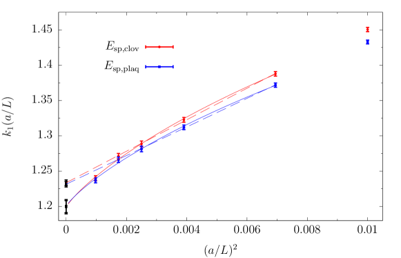
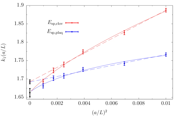
Figure 1: Continuum extrapolations for $k_{1}(a/L)$. Results for $c=0.3$ (upper panel) and $c=0.4$ (lower panel) are shown, for two different discretizations of the flow energy density.

In Fig. 1 we now present our results for $k_{1}(a/L)$ at $c=0.3$ and $0.4$. Two discretizations of the observable, namely clover and plaquette, are plotted. Focusing on the results for $c=0.3$, we first note that the statistical errors on $k_{1}(a/L)$ are around $4\cdot 10^{-3}$. In the plot we then show two different extrapolations to the continuum limit. In the first extrapolation (solid line), lattices with $L/a\geq 12$ are fitted to the asymptotic form (6) including the leading terms $m=2$, $n=0,1$. This results in a $\chi^{2}/{\rm d.o.f.}\sim 1$. A first important observation is that O($a^{2}$) effects are sizable, i.e. on the level of 0.1 at $L/a=10$. Secondly, the $m=2$, $n=1$, term is crucial to obtain a good fit of the data. In the second extrapolation (dashed line), instead, we considered lattices with $L/a\geq 12$ but excluded $L/a=32$. In this case the data can be very well described by a pure $(a/L)^{2}$ term over the whole range of lattice sizes. The continuum extrapolated value so obtained has smaller statistical errors, but is many standard deviations away from the result of the previous fit.

The results for $c=0.4$ exhibit qualitatively the same features, although the statistical errors of $k_{1}(a/L)$ are now $\sim 7\cdot 10^{-3}$ and the two discretizations of the observable show rather different lattice artifacts. On the other hand, cutoff effects are generally smaller than for $c=0.3$, and we thus included the $L/a=10$ data into the fits as well.

Given the above observations, we conclude that the extraction of continuum perturbative coefficients from NSPT data is rather delicate due to the presence of the logarithmic corrections to the continuum scaling. These are significant in the present case at a level of precision just below $10^{-2}$. Larger lattices are certainly needed to better constrain the observed behavior, and extract definite and reliable continuum results.

Accurate results are more difficult to obtain for the two-loop coefficient $k_{2}$ than for $k_{1}$. The statistical errors turn out to be about 10 times larger in this case and the extrapolation to the continuum limit is complicated by the presence of further terms in the fit function (cf. eq. (6)). A reliable analysis of the data for $k_{2}$ therefore has to wait for the ongoing simulations of larger (as well as some smaller) lattices to be completed.

5 Conclusions

In this contribution we investigated the possibility of using NSPT to compute the perturbative expansion of physical quantities in the continuum theory. To this end, we considered a non-trivial case: the determination of the two-loop matching between the GF coupling in finite-volume with SF boundary conditions and the $\overline{{\rm MS}}$ coupling, in the pure SU(3) gauge theory. The use of the SMD in place of the Langevin algorithm proves to be beneficial in this context and allows statistically precise results to be obtained near the continuum limit with a significantly reduced computational effort. In this respect, we note that an absolute uncertainty on the matching coefficients of $\sigma(k_{1})\sim 10^{-2}$ and $\sigma(k_{2})\sim 10^{-1}$, would imply a relative error on the determination of $\alpha_{\overline{\rm MS}}(m_{Z})$ around $0.2\%$ i.e. well below the error of state of the art non-perturbative determinations [24, 25].

Taking the continuum limit of the calculated coefficients can be challenging in view of the statistical uncertainties and the fact that the dependence on the lattice spacing is not simply power-like. Reliable extrapolations probably require O($a$)-improvement up to the order in the coupling considered and certainly accurate data over a significant range of lattice sizes extending up to some fairly large ones.

The inclusion of the quark fields in the SMD algorithm is in principle straightforward and is not expected to slow down the simulations by a large factor [10]. Different implementations are however possible, whose viability and efficiency will need to be determined.

6 Acknowledgments

M.D.B. has benefited from the pleasant collaboration with Marco Garofalo, Dirk Hesse, and Tony Kennedy on related investigations. He is also grateful to Alberto Ramos, Stefan Sint, and Rainer Sommer, for their valuable comments. The authors thank LRZ for the allocated computer time under the project id: pr92ci, as well as the computer centers at CERN and DESY – Zeuthen, for their precious support and resources.

References

- [1] M. Lüscher, JHEP 1008 (2010) 071. [Erratum: JHEP 03 (2014) 092.]
- [2] M. Lüscher and P. Weisz, JHEP 1102 (2011) 051.
- [3] M. Lüscher, PoS LATTICE2013 (2014) 016.
- [4] Z. Fodor et. al., JHEP 11 (2012) 007.
- [5] P. Fritzsch and A. Ramos, JHEP 1310 (2013) 008.
- [6] H. Suzuki, PTEP 2013 (2013) 083B03. [Erratum: PTEP 2015 (2015) 079201.]
- [7] E. I. Bribian and M. García Pérez, PoS LATTICE2016 (2017) 371.
- [8] R. V. Harlander and T. Neumann, JHEP 06 (2016) 161.
- [9] F. Di Renzo, E. Onofri, G. Marchesini, and P. Marenzoni, Nucl. Phys. B426 (1994) 675–685.
- [10] F. Di Renzo and L. Scorzato, JHEP 10 (2004) 073.
- [11] M. Dalla Brida and D. Hesse, PoS LATTICE2013 (2013) 326.
- [12] M. Dalla Brida, M. Garofalo, and A. D. Kennedy, PoS LATTICE2015 (2015) 309.
- [13] A. M. Horowitz, Phys. Lett. B156 (1985) 89.
- [14] A. M. Horowitz, Nucl. Phys. B280 (1987) 510.
- [15] M. Lüscher and S. Schaefer, JHEP 07 (2011) 036.
- [16] M. Lüscher and S. Schaefer, JHEP 04 (2011) 104.
- [17] M. Brambilla et al., PoS LATTICE2013 (2013) 325.
- [18] M. Lüscher, R. Narayanan, P. Weisz, and U. Wolff, Nucl. Phys. B384 (1992) 168–228.
- [19] M. Lüscher and P. Weisz, Nucl. Phys. B452 (1995) 234–260.
- [20] K. Symanzik, NATO Sci. Ser. B59 (1980) 313–330.
- [21] K. Symanzik, J. Phys. Colloq. 43 (1982) C3 254.
- [22] I. P. Omelyan, I. M. Mryglod, and R. Folk, Comp. Phys. Commun. 151 (2003) 272.
- [23] G. S. Bali, C. Bauer, A. Pineda, and C. Torrero, Phys. Rev. D87 (2013) 094517.
- [24] M. Dalla Brida et. al., Phys. Rev. Lett. 117 (2016), no. 18 182001.
- [25] M. Dalla Brida et. al., PoS LATTICE2016 (2017) 197.