ADP-16-46/T1002 DESY 16-241 Edinburgh 2016/19 Liverpool LTH 1116 December 14, 2016 Flavour breaking effects in the pseudoscalar meson decay constants

Abstract

The SU(3) flavour symmetry breaking expansion in up, down and strange quark masses is extended from hadron masses to meson decay constants. This allows a determination of the ratio of kaon to pion decay constants in QCD. Furthermore when using partially quenched valence quarks the expansion is such that SU(2) isospin breaking effects can also be determined. It is found that the lowest order SU(3) flavour symmetry breaking expansion (or Gell-Mann–Okubo expansion) works very well. Simulations are performed for 2+1 flavours of clover fermions at four lattice spacings.

1 Introduction

One approach to determine the ratio $|V_{us}/V_{ud}|$ of Cabibbo–-Kobayashi–-Maskawa (CKM) matrix elements, as suggested in [1], is by using the ratio of the experimentally determined pion and kaon leptonic decay rates

$${\Gamma(K^{+}\to\mu^{+}\nu_{\mu})\over\Gamma(\pi^{+}\to\mu^{+}\nu_{\mu})}=\left|{V_{us}\over V_{ud}}\right|^{2}\,\left(f_{K^{+}}\over f_{\pi^{+}}\right)^{2}\,{M_{K^{+}}\over M_{\pi^{+}}}\,\left(1-m_{\mu}^{2}/M^{2}_{K^{+}}\over 1-m_{\mu}^{2}/M^{2}_{\pi^{+}}\right)^{2}\,(1+\delta_{\rm em})\,,$$ (1)

(where $M_{K^{+}}$, $M_{\pi^{+}}$ and $m_{\mu}$ are the particle masses, and $\delta_{\rm em}$ is an electromagnetic correction factor). This in turn requires the determination of the ratio of kaon to pion decays constants, $f_{K^{+}}/f_{\pi^{+}}$, a non-perturbative task, where the lattice approach to QCD may be of help. For some recent work see, for example, [2, 3, 4, 5, 6, 7, 8, 9, 10].

The QCD interaction is flavour-blind and so when neglecting electromagnetic and weak interactions, the only difference between the quark flavours comes from the mass matrix. In this article we want to examine how this constrains meson decay matrix elements once full $SU(3)$ flavour symmetry is broken, using the same methods as we used in [11, 12] for hadron masses. In particular we shall consider pseudoscalar decay matrix elements and give an estimation for $f_{K}/f_{\pi}$ and $f_{K^{+}}/f_{\pi^{+}}$ (ignoring electromagnetic contributions).

2 Approach

In lattice simulations with three dynamical quarks there are many paths to approach the physical point where the quark masses take their physical values. The choice adopted here is to extrapolate from a point on the $SU(3)$ flavour symmetry line keeping the singlet quark mass $\overline{m}$ constant, as illustrated in the left panel of Fig. 1,

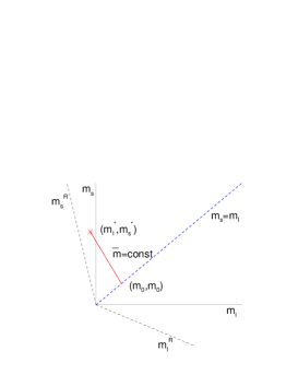
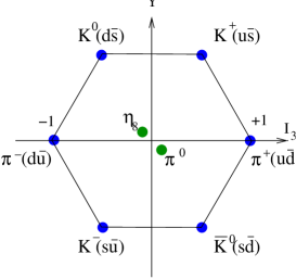
Figure 1: LH panel: Sketch of the path for the case of two mass degenerate quarks, $m_{u}=m_{d}\equiv m_{l}$, from a point on the $SU(3)$ flavour symmetric line $(m_{0},m_{0})$ to the physical point denoted with a ^∗: $(m_{l}^{*},m_{s}^{*})$. RH panel: The pseudoscalar octet meson.

for the case of two mass degenerate quarks $m_{u}=m_{d}\equiv m_{l}$. This allows the development of an $SU(3)$ flavour symmetry breaking expansion for hadron masses and matrix elements, i.e. an expansion in

$$\delta m_{q}=m_{q}-\overline{m}\,,\quad\mbox{with}\quad\overline{m}=\mbox{\small$\frac{1}{3}$}(m_{u}+m_{d}+m_{s})\,,$$ (2)

(where numerically $\overline{m}=m_{0}$). From this definition we have the trivial constraint

$$\delta m_{u}+\delta m_{d}+\delta m_{s}=0\,.$$ (3)

The path to the physical quark masses is called the ‘unitary line’ as we expand in the same masses for the sea and valence quarks. Note also that the expansion coefficients are functions of $\overline{m}$ only, which provided we keep $\overline{m}=\mbox{const.}$ reduces the number of allowed expansion coefficients considerably.

As an example of an $SU(3)$ flavour symmetry breaking expansion, [12], we consider the pseudoscalar masses, and find to next-to-leading-order, NLO, (i.e. $O((\delta m_{q})^{2})$).

$$M^{2}(a\overline{b}) = M^{2}_{0}+\alpha(\delta m_{a}+\delta m_{b})$$ (4)

$$\phantom{M^{2}_{0}}+\beta_{0}\mbox{\small$\frac{1}{6}$}(\delta m_{u}^{2}+\delta m_{d}^{2}+\delta m_{s}^{2})+\beta_{1}(\delta m_{a}^{2}+\delta m_{b}^{2})+\beta_{2}(\delta m_{a}-\delta m_{b})^{2}$$

$$\phantom{M^{2}_{0\pi}}+\ldots\,,$$

where $m_{a}$, $m_{b}$ are quark masses with $a,b=u,d,s$. This describes the physical outer ring of the pseudoscalar meson octet (the right panel of Fig. 1). Numerically we can also in addition consider a fictitious particle, where $a=b=s$, which we call $\eta_{s}$. We have further extended the expansion to the next-to-next-to-leading or NNLO case, [13]. As the expressions start to become unwieldy, they have been relegated to Appendix A. (Octet baryons also have equivalent expansions, [13].)

The vacuum is a flavour singlet, so meson to vacuum matrix elements $\langle 0|\widehat{\cal O}|M\rangle$ are proportional to $1\otimes 8\otimes 8$ tensors, i.e. $8\otimes 8$ matrices, where $\widehat{\cal O}$ is an octet operator. So the allowed mass dependence of the outer ring octet decay constants is similar to the allowed dependence of the octet masses. Thus we have

$$f(a\overline{b}) = F_{0}+G(\delta m_{a}+\delta m_{b})$$ (5)

$$\phantom{F_{0}}+H_{0}\mbox{\small$\frac{1}{6}$}(\delta m_{u}^{2}+\delta m_{d}^{2}+\delta m_{s}^{2})+H_{1}(\delta m_{a}^{2}+\delta m_{b}^{2})+H_{2}(\delta m_{a}-\delta m_{b})^{2}$$

$$\phantom{F_{0}}+\ldots\,.$$

The $SU(3)$ flavour symmetric breaking expansion has the simple property that for any flavour singlet quantity, which we generically denote by $X_{S}\equiv X_{S}(m_{u},m_{d},m_{s})$ then

$$X_{S}(\overline{m}+\delta m_{u},\overline{m}+\delta m_{d},\overline{m}+\delta m_{s})=X_{S}(\overline{m},\overline{m},\overline{m})+O((\delta m_{q})^{2})\,.$$ (6)

This is already encoded in the above pseudoscalar $SU(3)$ flavour symmetric breaking expansions, or more generally it can be shown, [11, 12], that $X_{S}$ has a stationary point about the $SU(3)$ flavour symmetric line.

Here we shall consider

$$X_{\pi}^{2} = \mbox{\small$\frac{1}{6}$}(M_{K^{+}}^{2}+M_{K^{0}}^{2}+M_{\pi^{+}}^{2}+M_{\pi^{-}}^{2}+M_{\overline{K}^{0}}^{2}+M_{K^{-}}^{2})\,,$$

$$X_{f_{\pi}} = \mbox{\small$\frac{1}{6}$}(f_{K^{+}}+f_{K^{0}}+f_{\pi^{+}}+f_{\pi^{-}}+f_{\overline{K}^{0}}+f_{K^{-}})\,.$$ (7)

(The experimental value of $X_{\pi}$ is $\sim 410\,\mbox{MeV}$, which sets the unitary range.) There are, of course, many other possibilities such as $S=N$, $\Lambda$, $\Sigma^{*}$, $\Delta$, $\rho$, $r_{0}$, $t_{0}$, $w_{0}$, [11, 12, 14].

As a further check, it can be shown that this property also holds using chiral perturbation theory. For example for mass degenerate $u$ and $d$ quark masses and assuming $\chi$PT is valid in the region of the $SU(3)$ flavour symmetric quark mass we find

$$X_{f_{\pi}}=f_{0}\left[1+{8\over f_{0}^{2}}(3L_{4}+L_{5})\overline{\chi}-3L(\overline{\chi})\right]+O((\delta\chi_{l})^{2})\,,$$ (8)

where the expansion parameter is given by $\delta\chi_{l}=\overline{\chi}-\chi_{l}$ with $\overline{\chi}=\textstyle{1\over 3}(2\chi_{l}+\chi_{s})$, $\chi_{l}=B_{0}m_{l}$, $\chi_{s}=B_{0}m_{s}$, $f_{0}$ is the pion decay constant in the chiral limit, $L_{i}$ are chiral constants and $L(\chi)=\chi/(4\pi f_{0})^{2}\times\ln(\chi/\Lambda_{\chi}^{2})$ is the chiral logarithm. In eq. (8), as expected, there is an absence of a linear term $\propto\delta\chi_{l}$.

The unitary range is rather small so we introduce PQ or partially quenching (i.e. the valence quark masses can be different to the sea quark masses). This does not increase the number of expansion coefficients. Let us denote the valence quark masses by $\mu_{q}$ and the expansion parameter as $\delta\mu_{q}=\mu_{q}-\overline{m}$. Then we have

$$\tilde{M}^{2}(a\overline{b}) = 1+\tilde{\alpha}(\delta\mu_{a}+\delta\mu_{b})$$ (9)

$$-(\mbox{\small$\frac{2}{3}$}\tilde{\beta}_{1}+\tilde{\beta}_{2})(\delta m_{u}^{2}+\delta m_{d}^{2}+\delta m_{s}^{2})+\tilde{\beta}_{1}(\delta\mu_{a}^{2}+\delta\mu_{b}^{2})+\tilde{\beta}_{2}(\delta\mu_{a}-\delta\mu_{b})^{2}$$

$$+\ldots\,,$$

and

$$\tilde{f}(a\overline{b}) = 1+\tilde{G}(\delta\mu_{a}+\delta\mu_{b})$$ (10)

$$-(\mbox{\small$\frac{2}{3}$}\tilde{H}_{1}+\tilde{H}_{2})(\delta m_{u}^{2}+\delta m_{d}^{2}+\delta m_{s}^{2})+\tilde{H}_{1}(\delta\mu_{a}^{2}+\delta\mu_{b}^{2})+\tilde{H}_{2}(\delta\mu_{a}-\delta\mu_{b})^{2}$$

$$+\ldots\,,$$

where in addition to the PQ generalisation we have also formed the ratios $\tilde{M}^{2}=M^{2}/X_{\pi}^{2}$, $\tilde{\alpha}=\alpha/M_{0}^{2}$, $\ldots$ and $\tilde{f}=f/X_{f_{\pi}}$, $\tilde{G}=G/F_{0}$, $\ldots\,$ (see Appendix A for the NNLO expressions). This will later prove useful for the numerical results. We see that there are mixed sea/valence mass terms at NLO (and higher orders). The unitary limit is recovered by simply replacing $\delta\mu_{q}\to\delta m_{q}$.

3 The Lattice

We use an $O(a)$ non-perturbatively improved clover action with tree level Symanzik glue and mildly stout smeared $2+1$ clover fermions, [15], for $\beta\equiv 10/g_{0}^{2}=5.40$, $5.50$, $5.65$, $5.80$ (four lattice spacings). We set

$$\mu_{q}={1\over 2}\left({1\over\kappa_{q}^{\rm val}}-{1\over\kappa_{0c}}\right)\,,$$ (11)

giving

$$\delta\mu_{q}=\mu_{q}-\overline{m}={1\over 2}\left({1\over\kappa_{q}^{\rm val}}-{1\over\kappa_{0}}\right)\,.$$ (12)

A $\kappa$ value along the $SU(3)$ symmetric line is denoted by $\kappa_{0}$, while $\kappa_{0c}$ is the value in the chiral limit. Note that practically we do not have to determine $\kappa_{0c}$, as it cancels in $\delta\mu_{q}$. (For simplicity we have set the lattice spacing to unity.)

We first investigate the constancy of $X_{S}$ in the unitary region. In Fig 2 we show various choices for $X_{S}$.

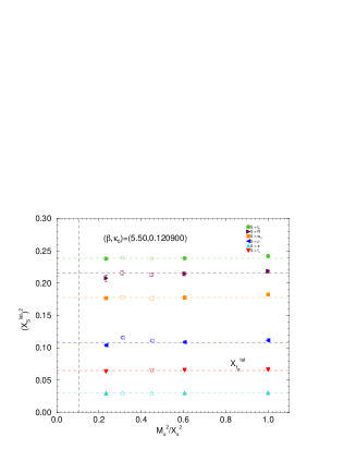
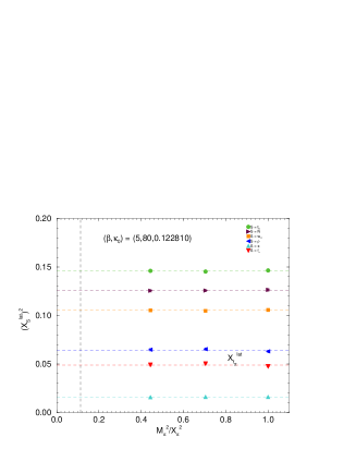
Figure 2: LH panel: $X^{2}_{t_{0}}$, $X^{2}_{w_{0}}$, $X^{2}_{\pi}$, $X^{2}_{\rho}$, $X^{2}_{N}\approx X^{2}_{\Lambda}$, $X_{f_{\pi}}$ for $(\beta,\kappa_{0})=(5.50,0.120900)$ along the $\overline{m}=\mbox{const.}$ line, together with constant fits. Open symbols have $M_{\pi}L\mathrel{\hbox to0.0pt{\lower 4.0pt\hbox{\hskip 1.0pt$\sim$}\hss}\raise 1.0pt\hbox{$<$}}4$ and are not included in the fit. The vertical line is the physical point. RH panel: The same for $(\beta,\kappa_{0})=(5.80,0.122810)$.

It is apparent that over a large range, starting from the $SU(3)$ flavour symmetric line, reaching down and approaching the physical point, $X_{S}$ appears constant, with very little evidence of curvature. (Although not included in the fits, the open symbols have $M_{\pi}L\sim 3$ – $4$ and also do not show curvature.) Presently our available pion masses reach down to $\sim 220\,\mbox{MeV}$.

Based on this observation, we determine the path in the quark mass plane by considering $M_{\pi}^{2}/X_{S}^{2}$ against $(2M_{K}^{2}-M_{\pi}^{2})/X_{S}^{2}$. If there is little curvature then we expect that

$${2M_{K}^{2}-M_{\pi}^{2}\over X^{2}_{S}}=3\,{X_{\pi}^{2}\over X_{S}^{2}}-2\,{M_{\pi}^{2}\over X_{S}^{2}}$$ (13)

holds for $S=N,\rho,t_{0},w_{0},\ldots$ . In Fig. 3

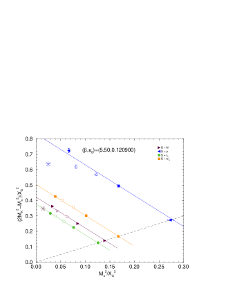
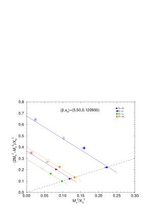
Figure 3: LH panel: $(2M_{K}^{2}-M_{\pi}^{2})/X_{S}^{2}$ versus $M_{\pi}^{2}/X_{S}^{2}$, $S=N$, $\rho$, $t_{0}$, $w_{0}$ for $(\beta,\kappa_{0})=(5.50,0.120900)$. Stars represent the physical points, the dashed line is the $SU(3)$ flavour symmetric line. RH panel: The same for $(\beta,\kappa_{0})=(5.50,0.120950)$.

we show this for $(\beta,\kappa_{0})=(5.50,0.120900)$, $(5.50,0.120950)$. We see that this is indeed the case. In addition $\kappa_{0}$ is adjusted so that the path goes through (or very close to) the physical value. For example we see that from the figure, $\beta=5.50$, $\kappa_{0}=0.120950$ is very much closer to this path than $\kappa_{0}=0.120900$, [14].

The programme is thus first to determine $\kappa_{0}$ and then find the expansion coefficients. Then use isospin symmetric ‘physical’ masses $M_{\pi}^{*}$, $M_{K}^{*}$ to determine $\delta m_{l}^{*}$ and $\delta m_{s}^{*}$. PQ results can help for the first task. As the range of PQ quark masses that can then be used is much larger than the unitary range, then the numerical determination of the relevant expansion coefficients is improved. PQ results were generated about $\kappa_{0}$, a single sea background, so $\tilde{\gamma}_{1}$ was not relevant. Also some coefficients (those $\propto(\delta\mu_{a}-\delta\mu_{b})^{2}$) often just contributed to noise, so were then ignored. In Fig. 4 we show $\tilde{M}_{\pi}^{2}$

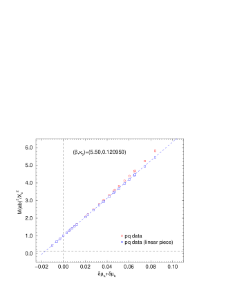
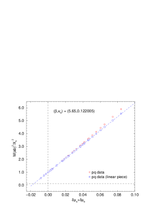
Figure 4: LH panel: PQ (and unitary) pseudoscalar mass results for $\tilde{M}^{2}=M^{2}/X_{\pi}^{2}$ with $(\beta,\kappa_{0})=(5.50,0.120950)$ against valence quarks $\delta\mu_{a}+\delta\mu_{b}$. The data is given by circles, while subtracting out the non-linear pieces (using the fit) gives the squares, together with the linear fit. The vertical dashed line is the symmetric point, while the horizontal dashed line represents the physical $\tilde{M}_{\pi}^{2}$. RH panel: Similarly for $(\beta,\kappa_{0})=(5.65,0.122005)$.

against $\delta\mu_{a}+\delta\mu_{b}$. From the $SU(3)$ flavour breaking expansions the leading-order or LO expansions are just a function of $\delta\mu_{a}+\delta\mu_{b}$; at higher orders, NLO etc. , this is not the case (see eq. (9)). We see that there is linear behaviour (coincidence of the PQ data with the linear piece) in the masses at least for $\tilde{M}_{\pi}^{2}\mathrel{\hbox to0.0pt{\lower 4.0pt\hbox{\hskip 1.0pt$\sim$}\hss}\raise 1.0pt\hbox{$<$}}3$ or $M_{\pi}\mathrel{\hbox to0.0pt{\lower 4.0pt\hbox{\hskip 1.0pt$\sim$}\hss}\raise 1.0pt\hbox{$<$}}\sqrt{3}\times 410\,\mbox{MeV}\sim 700\,\mbox{MeV}$. In Fig. 5 we show the corresponding results for

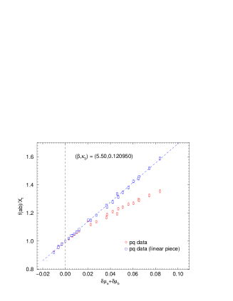
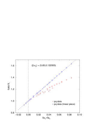
Figure 5: Similarly for the decay constant, $\tilde{f}=f/X_{f_{\pi}}$.

$\tilde{f}$. Again we see similar results for $\tilde{f}$ as for $\tilde{M}^{2}$; while our fit is describing the data well, the deviations from linearity occur earlier.

Furthermore the use of PQ results allows for a possibly interesting method for fine tuning of $\kappa_{0}$ to be developed. If we slightly miss the starting point on the $SU(3)$ flavour symmetric line, we can also tune $\kappa_{0}$ using PQ results so that we get the physical values of (say) $M^{*}_{\pi}$, $X^{*}_{N}$ and $M^{*}_{K}$ correct. This gives $\kappa_{0}$, $\delta\mu_{l}^{*}$, $\delta\mu_{s}^{*}$. The philosophy is that most change is due to a change in valence quark mass, rather than sea quark mass. Note that then $2\delta\mu_{l}^{*}+\delta\mu_{s}^{*}\not=0$ necessarily (while $2\delta m_{l}+\delta m_{s}$ always vanishes). For our $\kappa_{0}$ values used here, namely $(\beta,\kappa_{0})=(5.40,0.119930)$, $(5.50,0.120950)$, $(5.65,0.122005)$, $(5.80,0.122810)$, [14] (on $24^{3}\times 48$, $32^{3}\times 64$, $32^{3}\times 64$ and $48^{3}\times 96$ lattice volumes respectively) tests show this is a rather small correction and we shall use this as part of the systematic error, see Appendix C.

Of course the unitary range is much smaller, as can be seen from the horizontal lines in Fig. 4. In the LH panel of Fig. 6 we show this range as a

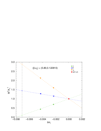
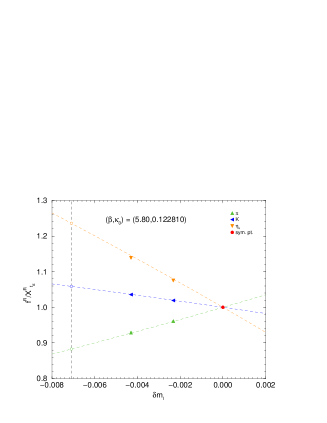
Figure 6: LH panel: Unitary results for $\tilde{M}^{2}=M^{2}/X_{\pi}^{2}$ versus $\delta m_{l}$ for $(\beta,\kappa_{0})=(5.80,0.122810)$. RH panel: Equivalent unitary results for $\tilde{f}=f/X_{f_{\pi}}$.

function of $\delta m_{l}$ for $\tilde{M}_{\pi}^{2}$, $\tilde{M}_{K}^{2}$ and $\tilde{M}_{\eta_{s}}^{2}$, together with the previously found fits. The expressions are given from eq. (9), setting $\delta\mu\to\delta m_{q}$ and then $a\to u$, $b\to d$ with $m_{u}=m_{d}\equiv m_{l}$ for $\tilde{M}^{2}_{\pi}$ etc. . Here we clearly observe the typical ‘fan’ behaviour seen in the mass of other hadron mass multiplets [12]. As we have mass degeneracy at the symmetric point, the masses radiate out from this point to their physical values. For both $\tilde{M}^{2}$ and $\tilde{f}$ the LO completely dominates.

As can be seen from Fig. 6 when $\tilde{M}_{\pi}$ takes its physical value, $\tilde{M}_{\pi}^{*}$, this determines the physical value $\delta m_{l}^{*}$. These are given in Table 1.

$\beta$	5.40	5.50	5.65	5.80
$\delta m_{l}^{*}$	-0.01041(11)	-0.008493(33)	-0.008348(33)	-0.007094(11)

Table 1: Results for $\delta m_{l}^{*}$.

Note that due to the constraint given in eq. (3) then $\delta m_{s}^{*}=-2\delta m_{l}^{*}$.

4 Decay constants

The renormalised and $O(a)$ improved axial current is given by [17]

$${\cal A}^{ab;{\mbox{\tiny$R$}}}_{\mu}=Z_{A}{\cal A}^{ab;{\mbox{\tiny$I\!M\!P$}}}_{\mu}\,,$$ (14)

with

$${\cal A}^{ab;\mbox{\tiny$I\!M\!P$}}_{\mu}=\left(1+\left[\overline{b}_{A}\overline{m}+\mbox{\small$\frac{1}{2}$}{b}_{A}(m_{a}+m_{b})\right]\right){\cal A}_{\mu}^{ab}\,,\qquad{\cal A}_{\mu}^{ab}=A^{ab}_{\mu}+c_{A}\partial_{\mu}P^{ab}\,,$$ (15)

and

$$A^{ab}_{\mu}=\overline{q}_{a}\gamma_{\mu}\gamma_{5}q_{b}\,,\qquad P^{ab}=\overline{q}_{a}\gamma_{5}q_{b}\,.$$ (16)

Using the axial current we first define matrix elements

$$\langle 0|\widehat{A}_{4}|M\rangle=M\,f\,,\qquad\langle 0|\widehat{\partial_{4}P}|M\rangle=M\,f^{(1)}\,,$$ (17)

giving for the renormalised pseudoscalar constants

$$f^{\mbox{\tiny$R$}}=Z_{A}\left(1+c_{A}{f^{(1)}\over f}\right)\left(1+\left[(\overline{b}_{A}+b_{A})\overline{m}+\mbox{\small$\frac{1}{2}$}b_{A}(\delta m_{a}+\delta m_{b})\right]\right)f\,.$$ (18)

As indicated in Fig. 7, we note that $c_{A}$ is small

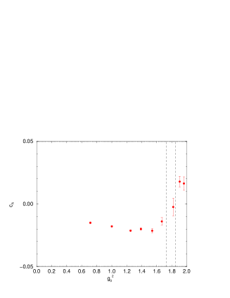
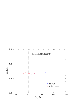
Figure 7: LH panel: Estimate of the $c_{A}$ improvement coefficient using the Schrödinger Functional, [15] as a function of $g_{0}^{2}=10/\beta$. The vertical dashed lines denote the $\beta$ range $5.40$ – $5.80$. RH panel: The ratio $f^{(1)}/f$ versus $\delta\mu_{a}+\delta\mu_{b}$ for $(\beta,\kappa_{0})=(5.80,0.122810)$.

(compared to unity) and that $f^{(1)}/f$ is constant and $\sim O(1)$ in the unitary region. So for constant $\overline{m}$ we can absorb the $c_{A}f^{(1)}/f$ and $(\overline{b}_{A}+b_{A})\overline{m}$ terms to give a change in the first coefficient

$$\tilde{f}^{\mbox{\tiny$R$}}\equiv{f^{\mbox{\tiny$R$}}\over X_{f_{\pi}}^{\mbox{\tiny$R$}}}=1+\left(\tilde{G}+\mbox{\small$\frac{1}{2}$}b_{A}\right)(\delta m_{a}+\delta m_{b})+\ldots\,.$$ (19)

For $b_{A}$ (only defined up to terms of $O(a)$) we presently take the tree level value, $b_{A}=1+O(g_{0}^{2})$.

5 Results

5.1 $f_{K}/f_{\pi}$

As demonstrated in the RH panel of Fig. 6, we again expect LO behaviour for $SU(3)$ flavour symmetry breaking for $\tilde{f}$ to dominate in the unitary region. Using the coefficients for the $SU(3)$ flavour breaking expansion for $\tilde{f}$ as previously determined, and then extrapolating to the physical quark masses gives the results in Table 2.

$\beta$	$a\,[\mbox{fm}]$	$\tilde{f}_{\pi}^{\mbox{\tiny$R$}*}$	$\tilde{f}_{K}^{\mbox{\tiny$R$}*}$	$\tilde{f}_{\eta_{s}}^{\mbox{\tiny$R$}*}$
5.40	0.0818(9)	0.8739(52)	1.0631(26)	1.2540(97)
5.50	0.0740(4)	0.8859(34)	1.0573(17)	1.2328(63)
5.65	0.0684(4)	0.8806(34)	1.0599(17)	1.2423(62)
5.80	0.0588(3)	0.8827(14)	1.0587(07)	1.2359(28)
$\infty$	0	0.8862(52)	1.0568(26)	1.2263(99)

Table 2: Results for $\tilde{f}_{\pi}^{\mbox{\tiny$R$}*}$, $\tilde{f}_{K}^{\mbox{\tiny$R$}*}$, $\tilde{f}_{\eta_{s}}^{\mbox{\tiny$R$}*}$, together with the extrapolated continuum value.

Finally using these results, we perform the final continuum extrapolation, using the lattice spacings given in [14], as shown in Fig. 8.

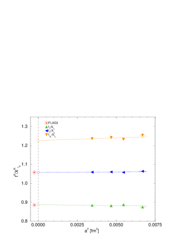
Figure 8: The continuum extrapolation of $\tilde{f}^{\mbox{\tiny$R$}*}$. The extrapolated values are again given as open circles. The converted FLAG3 values, [16], are given as stars.

(The fits have $\chi^{2}/{\rm dof}\sim 3.3/2\sim 1.6$.) For comparison, the FLAG3 values, [16], are shown as stars. (Note that although $f_{\eta_{s}}$ helps in determining the expansion coefficients, there is no further information to be found from the various extrapolated values.) Continuum values are also given in Table 2. Converting $\tilde{f}_{K}^{\mbox{\tiny$R$}*}$ gives a result of

$${f_{K}\over f_{\pi}}=1.192(10)(13)\,,$$ (20)

(for simplicity now dropping the superscripts). The first error is statistical; the second is an estimate of the combined systematic error due to $b_{A}$, $SU(3)$ flavour breaking expansion, finite volume and our chosen path to the physical point as discussed in Appendix C.

5.2 Isospin breaking effects

Finally we briefly discuss $SU(2)$ isospin breaking effects. Provided $\overline{m}$ is kept constant, then the $SU(3)$ flavour breaking expansion coefficients ($\tilde{\alpha}$, $\tilde{G}\,,\ldots$) remain unaltered whether we consider $1+1+1$ or $2+1$ flavours. So although our numerical results are for mass degenerate $u$ and $d$ quarks we can use them to discuss isospin breaking effects (ignoring electromagnetic corrections). We parameterise these effects by

$${f_{K^{+}}\over f_{\pi^{+}}}={f_{K}\over f_{\pi}}\left(1+\mbox{\small$\frac{1}{2}$}\delta_{SU(2)}\right)\,,$$

and expanding in $\Delta m=(\delta m_{d}-\delta m_{u})/2$ about the average light quark mass $\delta m_{l}=(\delta m_{u}+\delta m_{d})/2$ gives, using the LO expansions (which from Figs. 4, 5 or more particularly Fig. 6, have been shown to work well)

$$\delta_{SU(2)}={2\over 3}\left(1-\left({f_{K}\over f_{\pi}}\right)^{-1}\right){\Delta m\over\delta m_{l}}\,,$$ (21)

with

$${\Delta m\over\delta m_{l}}={3\over 2}\,{M_{K^{0}}^{2}-M_{K^{+}}^{2}\over M_{\pi^{+}}^{2}-\mbox{\small$\frac{1}{2}$}\left(M_{K^{0}}^{2}+M_{K^{+}}^{2}\right)}\,.$$ (22)

At the physical point, using the FLAG3, [16], mass values gives $\Delta m^{*}/\delta m_{l}^{*}$ and hence using our determined value for $f_{K^{+}}/f_{\pi^{+}}$, we find

$$\delta_{SU(2)}=-0.0042(2)(2)\,.$$ (23)

Alternatively, this gives

$${f_{K^{+}}\over f_{\pi^{+}}}=1.190(10)(13)\,.$$

6 Conclusions

We have extended our programme of tuning the strange and light quark masses to their physical values simultaneously by keeping the average quark mass constant from pseudoscalar meson masses to pseudoscalar decay constants. As for masses we find that the $SU(3)$ flavour symmetry breaking expansion, or Gell-Mann–Okubo expansion, works well even at leading order.

Further developments to reduce error bars could include another finer lattice spacing, as the extrapolation lever arm in $a^{2}$ is rather large and presently contributes substantially to the errors, and PQ results with sea quark masses not just at the symmetric point ($\kappa_{0}$) but at other points on the $\overline{m}=\mbox{const}.$ line.

Appendix

Appendix A Next-to next-to leading order expansion

We give here the next-to next-to leading order expansion or NNLO expansion for the octet pseudoscalars and decay constants, which generalise the results of eqs. (4), (9) and eqs. (5), (10). For the pseudoscalar mesons we have

$$M^{2}(a\overline{b}) = M^{2}_{0}+\alpha(\delta\mu_{a}+\delta\mu_{b})$$ (24)

$$+\beta_{0}\mbox{\small$\frac{1}{6}$}(\delta m_{u}^{2}+\delta m_{d}^{2}+\delta m_{s}^{2})+\beta_{1}(\delta\mu_{a}^{2}+\delta\mu_{b}^{2})+\beta_{2}(\delta\mu_{a}-\delta\mu_{b})^{2}$$

$$+\gamma_{0}\delta m_{u}\delta m_{d}\delta m_{s}+\gamma_{1}(\delta\mu_{a}+\delta\mu_{b})(\delta m_{u}^{2}+\delta m_{d}^{2}+\delta m_{s}^{2})$$

$$+\gamma_{2}(\delta\mu_{a}+\delta\mu_{b})^{3}+\gamma_{3}(\delta\mu_{a}+\delta\mu_{b})(\delta\mu_{a}-\delta\mu_{b})^{2}\,,$$

and

$$\tilde{M}^{2}(a\overline{b}) = 1+\tilde{\alpha}(\delta\mu_{a}+\delta\mu_{b})$$ (25)

$$-(\mbox{\small$\frac{2}{3}$}\tilde{\beta}_{1}+\tilde{\beta}_{2})(\delta m_{u}^{2}+\delta m_{d}^{2}+\delta m_{s}^{2})+\tilde{\beta}_{1}(\delta\mu_{a}^{2}+\delta\mu_{b}^{2})+\tilde{\beta}_{2}(\delta\mu_{a}-\delta\mu_{b})^{2}$$

$$+(2\tilde{\gamma}_{2}-6\tilde{\gamma}_{3})\delta m_{u}\delta m_{d}\delta m_{s}+\tilde{\gamma}_{1}(\delta\mu_{a}+\delta\mu_{b})(\delta m_{u}^{2}+\delta m_{d}^{2}+\delta m_{s}^{2})$$

$$+\tilde{\gamma}_{2}(\delta\mu_{a}+\delta\mu_{b})^{3}+\tilde{\gamma}_{3}(\delta\mu_{a}+\delta\mu_{b})(\delta\mu_{a}-\delta\mu_{b})^{2}\,.$$

where $\tilde{M}^{2}(a\overline{b})=M^{2}(a\overline{b})/X_{\pi}^{2}$ and for an expansion coefficient $\tilde{\alpha}=\alpha/M_{0}^{2}$, $\tilde{\beta}_{i}=\beta_{i}/M_{0}^{2}$, $i=1$, $2$, and $\tilde{\gamma}_{i}=\gamma_{i}/M_{0}^{2}$, $i=1$, $2$, $3$ and we have then redefined $\tilde{\gamma}_{1}$ by $\tilde{\gamma}_{1}-\tilde{\alpha}(\mbox{\small$\frac{1}{6}$}\tilde{\beta}_{0}+\mbox{\small$\frac{2}{3}$}\tilde{\beta}_{1}+\tilde{\beta}_{2})\to\tilde{\gamma}_{1}$.

The $SU(3)$ flavour breaking expansion is identical for the decay constants, we just replace $M_{0}^{2}\to F_{0}$, $\alpha\to G$, $\beta_{i}\to H_{i}$, $\gamma_{i}\to I_{i}$ in eq. (24) and $\tilde{\alpha}\to\tilde{G}$, $\tilde{\beta}_{i}\to\tilde{H}_{i}$, $\tilde{\gamma}_{i}\to\tilde{I}_{i}$ in eq. (25).

Appendix B Correlation functions

On the lattice we extract the pseudoscalar decay constant from two-point correlation functions. For large times we expect that

$$C_{A_{4}P}(t) = {1\over V_{S}}\,\langle\sum_{\vec{x}}\,A_{4}(\vec{x},t)\sum_{\vec{y}}\,P(\vec{y},t)\rangle$$ (26)

$$= {1\over 2M}\left[\langle 0|\widehat{A}_{4}|M\rangle\langle 0|\widehat{P}|M\rangle^{*}e^{-Mt}+\langle 0|\widehat{A}^{\dagger}_{4}|M\rangle^{*}\langle 0|\widehat{P}^{\dagger}|M\rangle e^{-M(T-t)}\right]$$

$$= -A_{A_{4}P}\left[e^{-Mt}-e^{-M(T-t)}\right]\,,$$

and

$$C_{PP}(t) = {1\over V_{S}}\,\langle\sum_{\vec{x}}\,P(\vec{x},t)\sum_{\vec{y}}\,P(\vec{y},t)\rangle$$ (27)

$$= {1\over 2M}\left[\langle 0|\widehat{P}|M\rangle\langle 0|\widehat{P}|M\rangle^{*}e^{-Mt}+\langle 0|\widehat{P}^{\dagger}|M\rangle^{*}\langle 0|\widehat{P}^{\dagger}|M\rangle e^{-M(T-t)}\right]$$

$$= A_{PP}\left[e^{-Mt}+e^{-M(T-t)}\right]\,,$$

where $A_{4}$ and $P$ are given in eq. (16). We have suppressed the quark indices, so the equations with appropriate modification are valid for both the pion and kaon. $V_{S}$ is the spatial volume and $T$ is the temporal extent of the lattice. To increase the overlap of the operator with the state (where possible) the pseudoscalar operator has been smeared using Jacobi smearing, and denoted here with a superscript, $S$ for Smeared. We now set

$$\langle 0|\widehat{A}_{4}|M\rangle = Mf$$

$$\langle 0|\widehat{\partial_{4}P}|M\rangle = -\sinh M\langle 0|\widehat{P}|M\rangle=Mf^{(1)}\,,$$ (28)

where $f$, $f^{(1)}$ are real and positive. By computing $C_{A_{4}P^{\mbox{\tiny$S$}}}$ and $C_{P^{\mbox{\tiny$S$}}P^{\mbox{\tiny$S$}}}$ we find for the matrix element of $\widehat{A}_{4}$,

$$Mf={\sqrt{2M}\times{A_{A_{4}P^{\mbox{\tiny$S$}}}\over A_{P^{\mbox{\tiny$S$}}P^{\mbox{\tiny$S$}}}}\times\sqrt{A_{P^{\mbox{\tiny$S$}}P^{\mbox{\tiny$S$}}}}}\,,$$ (29)

and for the matrix element of $\widehat{\partial_{4}P}$ we obtain from the ratio of the $C_{PP^{\mbox{\tiny$S$}}}$ and $C_{A_{4}P^{\mbox{\tiny$S$}}}$ correlation functions

$${f^{(1)}\over f}=\sinh M\times{A_{PP^{\mbox{\tiny$S$}}}\over A_{A_{4}P^{\mbox{\tiny$S$}}}}\,.$$ (30)

Some further details and formulae for other decay constants are given in [20, 21].

Appendix C Systematic errors

We now consider in this Appendix possible sources of systematic errors.

Uncertainty in $b_{A}$

Presently the improvement coefficient $b_{A}$ is only known perturbatively to leading order. We have estimated the uncertainty here by repeating the analysis with $b_{A}=0$ and $b_{A}=2$. This leads to a systematic error on $f_{K}/f_{\pi}$ of $\sim 0.008$.

$SU(3)$ flavour breaking expansion

We first note that for the unitary range as illustrated in Fig. 6, the ‘ruler test’ indicates there is very little curvature. This shows that the $SU(3)$ flavour breaking expansion is highly convergent. (Each order in the expansion is multiplied by a further power of $|\delta m_{l}|\sim 0.01$.) This is also indicated in Fig. 2, where our lowest pion mass there is $\sim 220\,\mbox{MeV}$. Such expansions are very good compared to most approaches available to QCD. Comparing the LO (linear) approximation with the non-linear fit gives an estimation of the systematic error. The comparison yields the estimate to be $\sim 0.004$ for $f_{K}/f_{\pi}$.

Finite lattice volume

All the results used in the analysis here have $M_{\pi}L\mathrel{\hbox to0.0pt{\lower 4.0pt\hbox{\hskip 1.0pt$\sim$}\hss}\raise 1.0pt\hbox{$>$}}4$. We also have generated some PQ data for $(\beta,\kappa_{0})=(5.80,0.122810)$ on a smaller lattice volume – $32^{3}\times 64$. (This still has $M_{\pi}L>4$.) Performing the analysis leads to small changes in $\tilde{f}$. Making a continuum extrapolation (which is most sensitive to just the $\beta=5.80$ point) and comparing the result with that of eq. (20) results in a systematic error of $\sim 0.005$.

Path to physical point

As discussed in section 3, we can further tune $\kappa_{0}$ using PQ results to get the physical values $M_{\pi}^{*}$, $X_{N}^{*}$ and $M_{K}^{*}$ correct, to give $\kappa_{0}$, $\delta\mu_{l}^{*}$, $\delta\mu_{s}^{*}$. Setting $\delta\overline{\mu}^{*}\equiv(2\delta\mu_{l}^{*}+\delta\mu_{s}^{*})/3$ then at LO this average is given by

$$\delta\overline{\mu}^{*}={1\over 2\tilde{\alpha}}\left(\left(\left.{X_{\pi}^{\rm lat\,2}\over X_{N}^{\rm lat\,2}}\right/{X_{\pi}^{*2}\over X_{N}^{*2}}\right)^{-1}-1\right)\,,$$ (31)

(while $2\delta m_{l}+\delta m_{s}$ is always $=0$). This gives for example for $\beta=5.80$, $\delta\overline{\mu}^{*}\sim-0.0001$. Changing $\delta m_{l}^{*}$ (or $\delta m_{s}^{*}$) by this and making a continuum extrapolation (which is again most sensitive to this point) and comparing the result with that of eq. (20) results in a systematic error of $\sim 0.009$.

Total systematic error

Including all these systematic errors in quadrature give a total systematic estimate in $f_{K}/f_{\pi}$ of $\sim 0.013$.

References

- [1] W. J. Marciano, Phys. Rev. Lett. 93 (2004) 231803, [arXiv:hep-ph/ 0402299].
- [2] S. Dürr et al., [BMW Collaboration], Phys. Rev. D81 (2010) 054507, [arXiv:1001.4692[hep-lat]].
- [3] Y. Aoki et al., [RBC and UKQCD Collaborations] Phys. Rev. D83 (2011) 074508, [arXiv:1011.0892[hep-lat]].
- [4] G. P. Engel et al., [BGR Collaboration], Phys. Rev. D85 (2012) 034508, [arXiv:1112.1601[hep-lat]].
- [5] A. Bazavov et al., [MILC Collaboration], Phys. Rev. Lett. 110 (2013) 172003, [arXiv:1301.5855[hep-ph]].
- [6] R. J. Dowdall et al., [HPQCD Collaboration], Phys. Rev. D88 (2013) 074504, [arXiv:1303.1670[hep-lat]].
- [7] A. Bazavov et al., [Fermilab Lattice and MILC Collaborations], Phys. Rev. D90 (2014) 074509, [arXiv:1407.3772[hep-lat]].
- [8] T. Blum et al., [RBC and UKQCD Collaborations], Phys. Rev. D93 (2016) 074505, [arXiv:1411.7017[hep-lat]].
- [9] N. Carrasco et al., [ETM Collaboration], Phys. Rev. D91 (2015) 074506, [arXiv:1411.7908[hep-lat]].
- [10] S. Dürr et al., arXiv:1601.05998[hep-lat].
- [11] W. Bietenholz et al., [QCDSF–UKQCD Collaborations], Phys. Lett. B690 (2010) 436, [arXiv:1003.1114[hep-lat]].
- [12] W. Bietenholz et al., [QCDSF–UKQCD Collaborations], Phys. Rev. D84 (2011) 054509, [arXiv:1102.5300[hep-lat]].
- [13] R. Horsley et al., [QCDSF–UKQCD Collaborations], Phys. Rev. D86 (2012) 114511, [arXiv:1206.3156[hep-lat]].
- [14] V. G. Bornyakov et al., [QCDSF–UKQCD Collaborations], arXiv:1508.05916[hep-lat].
- [15] N. Cundy et al., [QCDSF–UKQCD Collaborations], Phys. Rev. D79 (2009) 094507, [arXiv:0901.3302[hep-lat]].
- [16] S. Aoki et al., [FLAG Working Group], arXiv:1607.00299[hep-lat].
- [17] T. Bhattacharya et al., Phys. Rev. D73 (2006) 034504, [arXiv:hep-lat/0511014].
- [18] Y. Nakamura and H. Stüben, Proc. Sci. Lattice 2010 (2010) 040, arXiv:1011.0199[hep-lat].
- [19] R. G. Edwards and B. Joó, Nucl. Phys. Proc. Suppl. 140 (2005) 832, arXiv:hep-lat/0409003.
- [20] M. Göckeler et al., Phys. Rev. D57 (1998) 5562, [arXiv:hep-lat/9707021].
- [21] A. Ali Khan et al., Phys. Lett. B652 (2007) 150, [hep-lat/0701015].