Robust Multigrid for Cartesian Interior Penalty DG Formulations of the Poisson Equation in 3D

Abstract.

We present a polynomial multigrid method for the nodal interior penalty formulation of the Poisson equation on three-dimensional Cartesian grids. Its key ingredient is a weighted overlapping Schwarz smoother operating on element-centered subdomains. The MG method reaches superior convergence rates corresponding to residual reductions of about two orders of magnitude within a single V(1,1) cycle. It is robust with respect to the mesh size and the ansatz order, at least up to ${P=32}$. Rigorous exploitation of tensor-product factorization yields a computational complexity of $O(PN)$ for $N$ unknowns, whereas numerical experiments indicate even linear runtime scaling. Moreover, by allowing adjustable subdomain overlaps and adding Krylov acceleration, the method proved feasible for anisotropic grids with element aspect ratios up to 48.

1. Introduction

Discontinuous Galerkin (DG) methods combine multiple desirable properties of finite element and finite volume methods, including geometric flexibility, variable approximation order, straightforward adaptivity and suitability for conservation laws [4, 11]. Though traditionally focused on hyperbolic systems, the need for implicit diffusion schemes and application to other problem classes, such as incompressible flow and elasticity, led to a growing interest in DG methods and related solution techniques for elliptic equations [1, 17]. This paper is concerned with fast elliptic solvers based on the multigrid (MG) method. In the context of high-order spectral element and DG methods, several approaches have been proposed: polynomial or $p$-MG [9, 5, 10, 8], geometric or $h$-MG [7, 13, 14], and algebraic MG [16, 2]. The most efficient methods reported so far [2, 18] use block smoothers that can be regarded as overlapping Schwarz methods. This work presents a hybrid Schwarz/MG method for nodal interior penalty DG formulations of Poisson problems on 3D Cartesian grids. It extends the techniques put forward in [18, 19] and generalizes the approach to variable subdomain overlaps. The remainder of the paper is organized as follows: Section 2 briefly describes the discretization, Sec. 3 the multigrid technique, including the Schwarz smoother, and Sec. 4 presents the results of the assessment by means of numerical experiments. Section 5 concludes the paper.

2. Discontinuous Galerkin Method

We consider the Poisson equation

$$-\nabla^{2}u=f$$ (1)

in the periodic domain ${\Omega=[0,l_{x}]\times[0,l_{y}]\times[0,l_{z}]}$. For discretization, the domain is decomposed into cuboidal elements $\{\Omega^{e}\}$ forming a Cartesian mesh. The discrete solution $u_{h}$ is sought in the function space

$$\mathcal{V}_{h}=\left\{v\in L^{2}(\Omega):v|_{\Omega^{e}}\in\mathcal{P}_{P}^{3}(\Omega^{e})\quad\forall\Omega^{e}\subset\Omega\right\},$$ (2)

where $\mathcal{P}_{P}^{3}$ is the 3D tensor product of polynomials of at most degree $P$. To cope with discontinuity we introduce the interior surface ${\Gamma=\cup\Gamma^{f}}$ which is composed of the element interfaces $\{\Gamma^{f}\}$. Let $\Omega^{-}$ and $\Omega^{+}$ denote the elements adjacent to $\Gamma^{f}$ and, respectively, $\boldsymbol{n}^{-}$ and $\boldsymbol{n}^{+}$ their exterior normals, and $v^{-}$ and $v^{+}$ the restrictions of $v$ to the joint face from inside the elements. Then we define the average and jump operators as

$$\{\{\hskip 0.50003ptv\hskip 0.50003pt\}\}=\frac{1}{2}(v^{-}+v^{+}),\quad[[\hskip 0.50003ptv\hskip 0.50003pt]]=\boldsymbol{n}^{-}v^{-}+\boldsymbol{n}^{+}v^{+}.$$ (3)

Given these prerequisites, the interior penalty discontinuous Galerkin formulation can be stated as follows (see, e.g. [1]): Find ${u_{h}\in\mathcal{V}_{h}}$ such that for all ${v\in\mathcal{V}_{h}}$

$$\int_{\Omega}\nabla v\cdot\nabla u_{h}\mathrm{d}\Omega+\int_{\Gamma}\left([[\hskip 0.50003pt\nabla v\hskip 0.50003pt]]\cdot\{\{\hskip 0.50003ptu_{h}\hskip 0.50003pt\}\}+\{\{\hskip 0.50003ptv\hskip 0.50003pt\}\}\cdot[[\hskip 0.50003pt\nabla u_{h}\hskip 0.50003pt]]\right)\mathrm{d}\Gamma\\ +\int_{\Gamma}\mu[[\hskip 0.50003ptv\hskip 0.50003pt]]\cdot[[\hskip 0.50003ptu_{h}\hskip 0.50003pt]]=\int_{\Omega}vf\mathrm{d}\Omega\,,$$ (4)

where $\mu$ is a piece-wise constant penalty parameter that must be chosen large enough to ensure stability.

Although, in theory, any suitable basis in $\mathcal{V}_{h}$ can be chosen, we restrict ourselves to nodal tensor-product bases generated from the Lagrange polynomials to the Gauss-Legendre (GL) or Gauss-Legendre-Lobatto (GLL) points, respectively. The discrete solution is expressed in $\Omega^{e}$ as

$$u_{h}(\boldsymbol{x})|_{\Omega^{e}}=u^{e}(\boldsymbol{\xi}^{e}(\boldsymbol{x}))=\sum_{i,j,k=0}^{P}u_{ijk}^{e}\varphi_{i}(\xi)\varphi_{j}(\eta)\varphi_{k}(\zeta)\,,$$ (5)

where $\varphi_{i}$ denotes the 1D base functions and $\boldsymbol{\xi}^{e}(\boldsymbol{x})$ the transformation from ${\Omega^{e}}$ to the reference element ${[-1,1]^{3}}$. Each coefficient $u_{ijk}^{e}$ is associated with one local base function, which is globalized by zero continuation outside $\Omega^{e}$. Inserting these base functions in (4) for $v$ and applying GL or GLL quadrature, according to the chosen basis, yields the discrete equations

$$\underline{A}\,\underline{u}=\underline{f}$$ (6)

for the solution vector ${\underline{u}=[u_{ijk}^{e}]}$. Due to the Cartesian element mesh and the tensor-product ansatz (5) the system matrix assumes the tensor-product form

$$\underline{A}=\underline{M}_{z}\otimes\underline{M}_{y}\otimes\underline{L}_{x}+\underline{M}_{z}\otimes\underline{L}_{y}\otimes\underline{M}_{x}+\underline{L}_{z}\otimes\underline{M}_{y}\otimes\underline{M}_{x}\,$$ (7)

where $\underline{M}_{\ast}$, $\underline{L}_{\ast}$ are the 1D mass and stiffness matrices for ${\ast=x,y,z}$. Without going into detail we remark that $\underline{M}_{\ast}$ is positive diagonal, and $\underline{L}_{\ast}$ symmetric positive semi-definite and block tridiagonal for either basis choice. The rigorous exploitation of these properties is crucial for the efficiency of the overall method.

3. Multigrid Techniques

The tensor-product structure of (8) allows for a straight-forward extension of the multigrid techniques developed in [18] for the 2D case. In the following, we examine polynomial multigrid (MG) and multigrid-preconditioned conjugate gradients (MG-CG) both using an overlapping Schwarz method for smoothing.

3.1. Schwarz Method

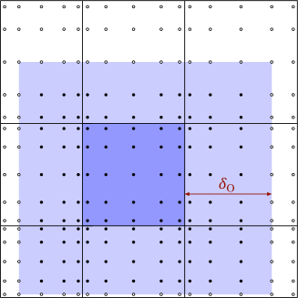
Schwarz methods are iterative domain decomposition techniques which improve the approximate solution by parallel or sequential subdomain solves, leading to additive or multiplicative methods, respectively. Here, we consider additive Schwarz with overlapping element-centered subdomains as sketched in Fig. 1. The overlap width $\delta_{\textsc{o}}$ can be different on each side of the embedded element, but may not exceed the width of the adjoining element. Alternatively, the overlap can be specified by prescribing the number $N_{\textsc{o}}$ of node layers adopted from the latter.

Figure 1. Element-centered subdomain. Every subdomain consists of a core region coinciding with the embedded element (dark) and an overlap zone (light shaded). The latter represents a strip of variable width $\delta_{\textsc{o}}$, which is adopted from the surrounding elements. The circles are the GL nodes for polynomial order ${P=4}$. Filled circles indicates the unknowns that are solved for.

To derive the subdomain problems, we first rewrite (8) into the residual form

$$\underline{A}\,\Delta\underline{u}=\underline{f}-\underline{A}\,\underline{\tilde{u}}=\underline{r}\,,$$ (8)

where ${\Delta\underline{u}=\underline{u}-\underline{\tilde{u}}}$ is the correction to the current approximate solution $\underline{\tilde{u}}$. For each subdomain $\Omega_{s}$ we define the restriction operator $\underline{R}_{s}$ such that ${\underline{u}_{s}=\underline{R}_{s}\underline{u}}$ gives the associated coefficients. Conversely, the transposed restriction operator, $\underline{R}_{s}^{\textsc{t}}$ globalizes the local coefficients by adding zeros for exterior nodes. With these prerequisites the correction contributed by $\Omega_{s}$ is defined as the solution to the subproblem

$$\underline{A}_{ss}\Delta\underline{u}_{s}=\underline{r}_{s}\,,$$ (9)

where $\underline{A}_{ss}=\underline{R}_{s}\underline{A}\,\underline{R}^{\textsc{t}}_{s}$ is the restricted system matrix and $\underline{r}_{s}=\underline{R}_{s}\underline{r}$ the restricted residual. Due to the cuboidal shape of the subdomain, the restriction operator possesses the tensor-product factorization ${\underline{R}_{s}=\underline{R}_{s,x}\otimes\underline{R}_{s,y}\otimes\underline{R}_{s,z}}$ and, as a consequence, $\underline{A}_{ss}$ inherits the tensor-structure of the full system matrix (7). Moreover it is regular and can be inverted using the fast diagonalization technique of Lynch et al. [15] to obtain

$$\underline{A}_{ss}^{-1}=(\underline{S}_{z}\otimes\underline{S}_{y}\otimes\underline{S}_{x})(\underline{I}\otimes\underline{I}\otimes\underline{\Lambda}_{x}+\underline{I}\otimes\underline{\Lambda}_{y}\otimes\underline{I}+\underline{\Lambda}_{z}\otimes\underline{I}\otimes\underline{I})^{-1}(\underline{S}_{z}^{\textsc{t}}\otimes\underline{S}_{y}^{\textsc{t}}\otimes\underline{S}_{x}^{\textsc{t}}),$$

where $\underline{S}_{\ast}$ is the column matrix of eigenvectors and $\Lambda_{\ast}$ the diagonal matrix of eigenvalues to the generalized eigenproblem for the restricted 1D stiffness and mass matrices and ${\ast=x,y,z}$. Exploiting this structure the solution can be computed in $O(P^{4})$ operations per subdomain.

One additive Schwarz iteration proceeds as follows: First, all subproblems are solved in parallel, which yields the local corrections ${\Delta\underline{u}_{s}}$. Afterwards, the global correction is computed as the weighted average

$$\Delta\underline{u}\simeq\sum_{s}\underline{R}_{s}^{\textsc{t}}(\underline{W}_{s}\Delta\underline{u}_{s})\,,$$ (10)

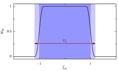
where ${\underline{W}_{s}=\underline{W}_{z}\otimes\underline{W}_{y}\otimes\underline{W}_{x}}$ is the diagonal local weighting matrix. The constituent 1D weights are computed from the hat-shaped weight function $w_{\textsc{h}}$, which is illustrated in Fig. 2. The complete definition of the weight function and alternative choices are given in [18].

Figure 2. Hat-shaped weight function using a piece-wise quintic transition from 0 at the subdomain boundary to 1 in the non-overlapped part of the core region. The coordinate $\xi_{\textsc{h}}$ coincides with $\xi$ inside the central element, and $\xi\mp 2$ in the left and right neighbor elements, respectively.

3.2. Multigrid and Preconditioned Conjugate Gradient Methods

For MG we define a series of polynomial levels $\{P_{l}\}$ with $P_{l}=2^{l}$ increasing from $1$ at $l=0$ to $P$ at top level $L$. Correspondingly, let $\underline{u}_{l}$ denote the global coefficients and $\underline{A}_{l}$ the system matrix on level $l$. On the top level we have $\underline{u}_{L}=\underline{u}$ and $\underline{A}_{L}=\underline{A}$, whereas on lower levels $\underline{u}_{l}$ is the defect correction and $\underline{A}_{l}$ the counterpart of $\underline{A}$ obtained with elements of order $P_{l}$. For transferring the correction from level $l-1$ to level $l$ we use the embedded interpolation operator $\underline{\mathcal{I}}_{l}$, and for restricting the residual its transpose. These ingredients allow to build the multigrid V-cycle summarized in Algorithm 1, where the Smoother represents the weighted additive Schwarz method. To allow for variable V-cycles [3], the number of pre- and post-smoothing steps, $N_{\textsc{s}1,l}$ and $N_{\textsc{s}2,l}$, may change from level to level. Line 11 of Algorithm 1 defines the coarse grid solution formally by means of the pseudoinverse $\underline{A}_{0}^{+}$. In our implementation the coarse problem is solved using the conjugate gradient method. To ensure convergence, the right side is projected to the null space of $\underline{A}_{0}$, as proposed in [12].

Algorithm 1 Multigrid V-cycle.

1:function MultigridCycle($\underline{u}$, $\underline{f}$, $\underline{N_{\textsc{s}}}$)

2:     $\underline{u}_{L}\leftarrow\underline{u}$

3:     $\underline{f}_{L}\leftarrow\underline{f}$

4:     for $l=L,1$ step $-1$ do

5:         if $l<L$ then

6:              $\underline{u}_{l}\leftarrow 0$

7:         end if

8:         $\underline{u}_{l}\leftarrow$ Smoother($\underline{u}_{l}$, $\underline{f}_{l}$, $N_{\textsc{s}1,l}$) $\triangleright$ Pre-smoothing

9:         $\underline{f}_{l-1}\leftarrow\underline{\mathcal{I}}^{\textsc{t}}_{l}(\underline{f}_{l}-\underline{A}_{l}\underline{u}_{l})$ $\triangleright$ Residual restriction

10:     end for

11:     $\underline{u}_{0}\leftarrow\underline{A}_{0}^{+}\underline{f}_{0}$ $\triangleright$ Coarse grid solution

12:     for $l=1,L$ do

13:         $\underline{u}_{l}\leftarrow\underline{u}_{l}+\underline{\mathcal{I}}_{l}\underline{u}_{l-1}$ $\triangleright$ Correction prolongation

14:         $\underline{u}_{l}\leftarrow$ Smoother($\underline{u}_{l}$, $\underline{f}_{l}$, $N_{\textsc{s}2,l}$) $\triangleright$ Post-smoothing

15:     end for

16:     return $\underline{u}\leftarrow\underline{u}_{L}$

17:end function

It is well known that the robustness of multigrid method can be enhanced by Krylov acceleration [20]. Here we use the inexact preconditioned conjugate gradient method [6], which copes with the asymmetry introduced by the weighted Schwarz method without imposing significant extra cost in comparison to conventional CG. A detailed description of the algorithm is given in [18].

4. Results

For assessing robustness and efficiency, the described methods were implemented in Fortran and applied to the $2\pi$-periodic Poisson problem with the exact solution

$$u(\boldsymbol{x})=\cos(x-3x+2z)\sin(1+x)\sin(1-x)\sin(2x+x)\sin(3x-2y+2z).$$

To keep the test series manageable, we constrained ourselves to equidistant grids with an identical number of elements in each direction. Anisotropic meshes were realized be choosing the domain extensions as multiples of $2\pi$, i.e. ${l_{\ast}=2\pi s_{\ast}}$, which yields the aspect ratio ${\Delta x:\Delta y:\Delta z=s_{x}:s_{y}:s_{z}}$. All tests started from a random guess confined to ${[-1,1]}$ and used a penalty parameter of ${\mu_{\ast}=2\mu_{\min,\ast}}$, where $\mu_{\min,\ast}$ is the stability threshold, e.g., $\mu_{\min,x}=P(P+1)/\Delta x$ for the $x$ direction [18]. The program was compiled using the Intel Fortran compiler 17.0 with optimization −O3 and run on a 3.1 GHz Intel Core i7-5557U CPU.

The primary assessment criterium is the average multigrid convergence rate

$$\rho=\sqrt[n]{\frac{r_{n}}{r_{0}}}\,,$$

where $r_{n}$ is the Euclidean norm of the residual vector after the $n$th cycle. Additionally we consider the number of cycles $n_{10}$ and the average runtime per unknown $\tau_{10}$ that are required to reduce the residual by a factor of $10^{10}$. These quantities follow from the convergence rate by ${n_{10}}=\lceil-10/\lg\rho\rceil$ and ${\tau_{10}=-10\,t_{\textsc{c}}/\lg\rho}$, respectively, where $t_{\textsc{c}}$ is the time required for one V-cycle.

4.1. Isotropic Meshes

First we consider the isotropic case with ${s_{x}=s_{y}=s_{z}=1}$, such that ${\Omega=[0,2\pi]^{3}}$. For assessing the impact of the subdomain overlap on the convergence rate and computational cost, we performed a test series for ansatz orders ${P=4}$ to $32$ using a degree-dependent tessellation into ${N_{\textsc{e}}=(128/P)^{3}}$ elements. Table 1 presents the logarithmic convergence rates for 14 test cases featuring different choices for the basis functions (GLL or GL), the solution method (MG or MG-CG) and the subdomain overlap. Note that the latter was chosen identical in each direction, because of mesh isotropy. All cases employed a fixed V-cycle with one pre- and post-smoothing step. Independent of the basis and the solution method, choosing a minimal overlap of just one node (${N_{\textsc{o}}=1}$) yields acceptable convergences rates for low order (${P=4}$), but becomes inefficient with increasing order. Using a geometrically fixed overlap of just eight percent of the element width (${\delta_{\textsc{o}}=0.08\Delta x}$) on every mesh level ensures robustness with respect to the ansatz order and even improves the convergence with growing $P$. Enlarging the overlap increases the convergence rate but also the computational cost, as will be detailed in a moment. Using Krylov acceleration tends to give faster convergence, however, this advantage melts away when increasing the overlap or the ansatz order. While these properties are consistently observed with the GLL basis, the GL results follow a less regular pattern and exhibit mostly lower convergence rates. This behavior can partly be explained by the fact that, with Gauss points, using a geometrically specified overlap width may result in zero overlapped node layers. While this phenomenon appears only at low orders, the latter are always present in the multigrid scheme, even at high ansatz orders. A remedy to this problem is to apply a lower bound of ${N_{\textsc{o},l}=1}$ for the nodal overlap on every mesh level $l$. Nevertheless, the GL-based approach remains slightly less efficient in comparison with the GLL approach. Therefore, further discussion will be constrained to the latter.

Table 1. Convergence rates obtained with different multigrid methods on isotopic meshes composed of $(128/P)^{3}$ elements for increasing ansatz order $P$.

					$\bar{r}=-\lg\rho$
#	Basis	Solver	Overlap	$N_{\textsc{o}}$	$P\!=\!4$	$P\!=\!8$	$P\!=\!16$	$P\!=\!32$
1	GLL	MG	$N_{\textsc{o}}=1$	$1,1,1,1,1$	1.08	0.89	0.46	0.24
2	GLL	MG-CG	$N_{\textsc{o}}=1$	$1,1,1,1,1$	1.34	1.21	0.80	0.52
3	GLL	MG	$\delta_{\textsc{o}}=0.08\Delta x$	$1,1,2,3,6$	1.08	1.59	2.13	2.82
4	GLL	MG-CG	$\delta_{\textsc{o}}=0.08\Delta x$	$1,1,2,3,6$	1.34	1.85	2.24	2.81
5	GLL	MG	$\delta_{\textsc{o}}=0.50\Delta x$	$2,3,5,9,17$	2.26	2.76	3.18	3.66
6	GLL	MG-CG	$\delta_{\textsc{o}}=0.50\Delta x$	$2,3,5,9,17$	2.29	2.67	3.08	3.75
7	GL	MG	$N_{\textsc{o}}=1$	$1,1,1,1,1$	0.73	0.96	0.73	0.40
8	GL	MG-CG	$N_{\textsc{o}}=1$	$1,1,1,1,1$	1.49	1.26	1.07	0.78
9	GL	MG	$\delta_{\textsc{o}}=0.08\Delta x$	$0,1,1,3,6$	0.73	1.15	1.70	2.20
10	GL	MG-CG	$\delta_{\textsc{o}}=0.08\Delta x$	$0,1,1,3,6$	1.14	1.38	1.84	2.15
11	GL	MG	$\delta_{\textsc{o}}=0.50\Delta x$	$1,2,4,8,16$	1.83	2.28	1.52	0.94
12	GL	MG-CG	$\delta_{\textsc{o}}=0.50\Delta x$	$1,2,4,8,16$	1.90	2.34	1.88	1.37
13	GL	MG	$\delta_{\textsc{o}}=0.09\Delta x$, $N_{\textsc{o}}\geq 1$	$1,1,2,3,6$	1.36	1.75	1.87	2.21
14	GL	MG-CG	$\delta_{\textsc{o}}=0.09\Delta x$, $N_{\textsc{o}}\geq 1$	$1,1,2,3,6$	1.49	1.81	2.03	2.22

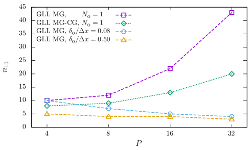
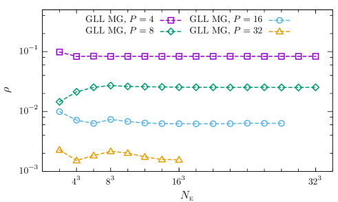
Complementary to the tabulated results, Fig. 3 depicts the number $n_{10}$ of multigrid cycles that are required to reduce the Euclidian residual norm by ten orders of magnitude for selected cases listed in Tab. 1. In agreement with the above discussion, the cycle count increases considerably when using GLL MG with only one node layer overlap. Adding Krylov acceleration (MG-CG) ameliorates this drawback, especially at higher order. Yet, pure MG with a fixed geometric overlap of 8 percent is far more efficient and even attains a decreasing $n_{10}$ with growing $P$. As expected, using an overlap of $\Delta x$$/$$2$ yields a further reduction of the cycle count. This advantage is, however, bought with additional computational cost related to the larger subdomain operator $\underline{A}_{ss}$. Figure 4 confirms that GLL MG with ${\delta_{\textsc{o}}=0.08\Delta x}$ outpaces the other choices for all polynomial degrees but 4, where the Krylov-accelerated method (MG-CG) with one node overlap is slightly faster. Moreover, Fig. 5 illustrates the robustness of this method with respect to the mesh size. With ansatz orders up to 16, the convergence rate becomes mesh independent for ${N_{\textsc{e}}\gtrsim 12^{3}}$, whereas it still tends to improve beyond ${N_{\textsc{e}}=16^{3}}$ for ${P=32}$. It is further worth noting that the convergence rates improves with growing order, reaching an excellent ${\rho\approx 6.3\times 10^{-3}}$ with ${P=16}$ and even better ${\rho\approx 1.6\times 10^{-3}}$ with ${P=32}$. Moreover, runtimes of about $3.5$ µs per degree of freedom allow to solve problems up to a million unknowns conveniently on a single core.

Figure 3. Number of cycles required to reduce the residual by ten orders of magnitude for selected methods listed in Tab. 1.

Figure 4. Runtime per unknown required to reduce the residual by ten orders of magnitude for selected methods listed in Tab. 1.

Figure 5. Convergence rates for GLL MG with overlap ${\delta_{\textsc{o}}=0.08\Delta x}$ for different orders $P$ displayed as a function of the mesh size.

4.2. Anisotropic Meshes

As a second issue we investigated the suitability of the approach for anisotropic meshes. For this purpose, we defined a sequence of domains

$$\Omega=(0,2\pi\,AR)\times(0,2\pi\lceil\,AR/2\rceil)\times(0,2\pi),\quad$$

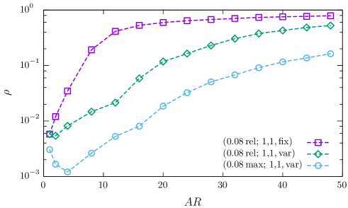
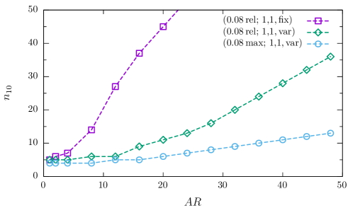
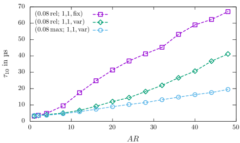
with aspect ratios $AR$ ranging from 1 to 48. Using a uniform tessellation featuring the same number of elements in each coordinate direction, $AR$ also represents the maximum element side aspect ratio. Thus, for example, ${AR=32}$ results in ${\Delta x=2\Delta y=32\Delta z}$. In earlier 2D studies, Krylov acceleration and variable V-cycles proved helpful, though yet insufficient, for coping with anisotropy. Based on this experience, we selected methods with different overlap and smoothing strategies, which are summarized in Tab. 2. Methods (0.08 rel; 1,1, fix) and (0.08 rel; 1,1, var) both use a relative subdomain overlap of 8 percent, which means that the overlap width varies in each coordinate direction proportionally to the corresponding element extension. In contrast, (0.08 max; 1,1, var) sets the overlap width to 8 percent of the maximal side length, but not larger than the element width in the given direction. Additionally, the last two methods apply a variable V-cycle, which increases the number of smoothing steps by a factor of 3 with each coarser level. The performance of these methods was studied on a $8^{3}$ tessellation using elements of order ${P=16}$. Figure 6 depicts the obtained convergence rates, cycle counts and runtimes per unknown for aspect ratios up to 48. With method (0.08 rel; 1,1, fix) convergence starts to degrade at moderate aspect ratios and has already slowed by to orders of magnitude at ${AR=16}$. Using a variable V-cycle improves the robustness such that a nearly constant cycle count $n_{10}$ is maintained until ${AR=12}$. From here convergence degrades more quickly, but remains superior to the previous case. Setting the overlap proportional to the largest element extension, as with method (0.08 max; 1,1, var), yields a further improvement, which becomes even more pronounced in the range ${AR>12}$, where the overlap in the most compressed direction is already constrained by the element width. Compared to the isotropic case, the cycle count grew from 4 to 13 at ${AR=48}$, whereas the serial runtime increased by factor of 5.4 to approximately 19 µs per unknown. This seems to be a good starting point, given the prospect of further acceleration, e.g. by parallelization.

Table 2. Test cases for investigating the robustness against the element aspect ratio.

Case	Subdomain overlap	Smoothing steps
(0.08 rel; 1,1, fix)	$\delta_{\textsc{o},\,x_{i}}=0.08\Delta x_{i}$	$N_{\textsc{s},l}=(1,1)$
(0.08 rel; 1,1, var)	$\delta_{\textsc{o},\,x_{i}}=0.08\Delta x_{i}$	$N_{\textsc{s},l}=(1,1)\times 3^{L-l}$
(0.08 max; 1,1, var)	$\delta_{\textsc{o},\,x_{i}}=\min[\max_{j}(0.08\Delta x_{j}),\,\Delta x_{i}]$	$N_{\textsc{s},l}=(1,1)\times 3^{L-l}$

(a) Multigrid convergence rates depending on the aspect ratio for methods listed in Tab. 2.

(b) Cycle counts depending on the aspect ratio for methods listed in Tab. 2.

(c) Runtime per unknown depending on the aspect ratio for methods listed in Tab. 2.

Figure 6. Results for varying element aspect ratios.

5. Conclusions

We developed a polynomial multigrid method for nodal interior-penalty formulations of the Poisson equation on three-dimensional Cartesian grids. Its key ingredient is an overlapping weighted Schwarz smoother, which exploits the underlying tensor-product structure for fast solution of the subdomain problems. The method achieves excellent convergence rates and proved robust against the mesh size and ansatz orders up to at least 32. Extending the ideas put forward in [18], we showed that combining Krylov acceleration, variable smoothing and increasing the subdomain overlap proportionally to the maximum element width improves the robustness considerably and renders the approach feasible for aspect ratios up to 50. Moreover, the method is computationally efficient, allowing to solve problems with a million unknowns in a few seconds on a single CPU core.

References

- [1] Arnold DN, Brezzi F, Cockburn B, Marini LD (2001) Unified analysis of discontinuous Galerkin methods for elliptic problems. SIAM J Numer Anal, 39(5):1749–1779
- [2] Bastian P, Blatt M, Scheichl R (2012) Algebraic multigrid for discontinuous Galerkin discretizations of heterogeneous elliptic problems. Numer Linear Algebra Appl, 19:367–388
- [3] Bramble J (1995) Multigrid methods. Pitman Res. Notes Math. Ser. 294. Longman Scientific & Technical, Harlow, UK
- [4] Cockburn B, Karniadakis GE, Shu C-W (2000) Discontinuous Galerkin Methods: Theory, Computation and Applications. Springer Berlin Heidelberg
- [5] Fidkowski KJ, Oliver TA, Lu J, Darmofal DL (2005) -multigrid solution of high-order discontinuous Galerkin discretizations of the compressible Navier-Stokes equations. J Comput Phys, 207:92–113
- [6] Golub GH, Ye Q (1999) Inexact preconditioned conjugate gradient method with inner-outer iteration. SIAM J Sci Comput, 21(4):1305–1320
- [7] Gopalakrishnan J, Kanschat G (2003) A multilevel discontinuous Galerkin method. Numer Math, 95:527–550
- [8] Haupt L, Stiller J, Nagel W (2013) A fast spectral element solver combining static condensation and multigrid techniques. J Comput Phys, 255:384–395
- [9] Helenbrook BT, Atkins HL, Mavriplis DJ (2003) Analysis of -multigrid for continuous and discontinuous finite element discretizations. AIAA Paper 2003-3989
- [10] Helenbrook BT, Atkins HL (2006) Application of -multigrid to discontinuous Galerkin formulations of the poisson equation. AIAA J, 44:566–575
- [11] Hesthaven JS, Warburton T (2008) Nodal Discontinuous Galerkin Methods. Springer
- [12] Kaasschieter EF (1988) Preconditioned conjugate gradients for solving singular systems. J Comput Appl Math, 24:265–275
- [13] Kanschat G (2004) Multilevel methods for discontinuous Galerkin FEM on locally refined meshes. Computers and Structures, 82:2437–2445
- [14] Kraus JK, Tomar SK (2008) A multilevel method for discontinuous Galerkin approximation of three-dimensional anisotropic elliptic problems. Numer Linear Algebra Appl, 15:417–438
- [15] Lynch RE, Rice JR, Thomas DH (1964) Direct solution of partial difference equations by tensor product methods. Numer Math, 6:185–199
- [16] Olson LN Schroder JB (2011) Smoothed aggregation multigrid solvers for high-order discontinuous Galerkin methods for elliptic problems. J Comput Phys, 230:6959–6976
- [17] Rivière B (2008) Discontinuous Galerkin Methods for Solving Elliptic and Parabolic Equations: Theory and Implementation. Frontiers in Mathematics, Vol. 35, SIAM, Philadelphia, PA, USA
- [18] Stiller J (2016) Robust multigrid for high-order discontinuous Galerkin methods: A fast Poisson solver suitable for high-aspect ratio Cartesian grids. J Comput Phys, 327:317–336
- [19] Stiller J (2017) Nonuniformly weighted Schwarz smoothers for spectral element multigrid. J Sci Comput (revised version in review)
- [20] Trottenberg U, Oosterlee CW, Schüller A (2000) Multigrid. Academic Press