Stationary Expansion Shocks for a Regularized Boussinesq System

Abstract

Stationary expansion shocks have been recently identified as a new type of solution to hyperbolic conservation laws regularized by non-local dispersive terms that naturally arise in shallow-water theory. These expansion shocks were studied in [1] for the Benjamin-Bona-Mahony equation using matched asymptotic expansions. In this paper, we extend the analysis of [1] to the regularized Boussinesq system by using Riemann invariants of the underlying dispersionless shallow water equations. The extension for a system is non-trivial, requiring a combination of small amplitude, long-wave expansions with high order matched asymptotics. The constructed asymptotic solution is shown to be in excellent agreement with accurate numerical simulations of the Boussinesq system for a range of appropriately smoothed Riemann data.

1 Introduction

We consider the normalized form of the classical regularized Boussinesq system for shallow water waves with dispersion (see e.g. [2], [3])

$$\begin{array}[]{rcl}h_{t}+(uh)_{x}&=&0\\[6.0pt] u_{t}+uu_{x}+h_{x}-{\textstyle{1\over 3}}u_{xxt}&=&0,\end{array}$$ (1)

The non-dimensional variables $h,u$ represent the height of the water free surface above a flat horizontal bottom, and the depth-averaged horizontal component of the water velocity, respectively. System (1) is non-evolutionary, i.e. not explicitly resolvable with respect to the time derivatives, a property that admits the possibility of new classes of solutions not generally observed in hyperbolic conservation laws and their evolutionary dispersive regularizations such as the Korteweg - de Vries equation, the defocusing nonlinear Schrödinger equation, and other equations exhibiting rich families of dispersive shock waves [4, 5]. New solutions in the form of stationary, smooth, non-oscillatory expansion shocks were found in [1] for the Benjamin-Bona-Mahony (BBM) equation, that represents a uni-directional analog of the system (1).

A stationary shock solution of (1),

$$h(x,t)=\left\{\begin{array}[]{ll}h_{-},&x<0\\[6.0pt] h_{+},&x>0,\end{array}\right.\ \ \ u(x,t)=\left\{\begin{array}[]{ll}u_{-},&x<0\\[6.0pt] u_{+},&x>0,\end{array}\right.$$ (2)

must satisfy Rankine-Hugoniot (RH) jump conditions

$$h_{+}u_{+}=h_{-}u_{-};\ \ h_{+}+{\textstyle{1\over 2}}u_{+}^{2}=h_{-}+{\textstyle{1\over 2}}u_{-}^{2}.$$ (3)

Equations (3) can be reformulated to express $u_{\pm}$ in terms of $h_{\pm}$ yielding expressions that we refer to as the RH locus

$$u_{\pm}=h_{\mp}\left(\frac{2}{h_{-}+h_{+}}\right)^{1/2}.$$ (4)

Note that (2), (3) is a weak solution of both the hyperbolic system of dispersionless shallow-water equations and the dispersive system (1), due to the shock being time-independent. The shock is expansive (in the sense specified below) if and only if $h_{+}<h_{-}$. Expansion shocks do not satisfy Lax entropy conditions [6] and are known to be unstable, immediately giving way to continuous self-similar rarefaction waves in hyperbolic theory. However, for certain types of dispersive regularization, a smoothed stationary expansion shock can persist, exhibiting only slow, algebraic decay with time. This new type of shock wave was identified in the BBM equation [1] by constructing an asymptotic solution of an initial value problem with smoothed jump (Riemann) initial data.

In [1], we also showed numerical simulations of the Boussinesq system (1) with initial conditions for $h,u$ representing smoothed Riemann data with $h_{+}<h_{-}$ satisfying the Rankine-Hugoniot conditions (3) in the far field. The graphs of the variables $h(x,t),u(x,t)$ as time $t$ evolves resemble the structures observed for the evolution of the asymptotic solution of the BBM equation [1]. However, the arguments of that paper do not apply directly to the evolution of stationary shocks for the system (1), and the purpose of this paper is to show how the BBM analysis can be extended to describe the Boussinesq expansion shocks. It turns out that the generalization of the analysis of [1] to a system requires some subtle manipulations, including expansions with two parameters and a higher order matched asymptotic analysis. The analysis reveals features of the solution not present in the scalar case. The central idea is to use Riemann invariants of the underlying dispersionless shallow water system as new field variables in the full dispersive equations (1). Broadly speaking, the Riemann invariant associated with the faster characteristic speed is constant to a high order, while the Riemann invariant of the slower characteristic speed evolves according to the BBM equation. However, a consistent characterization of this broad behavior requires a careful use of matched asymptotic expansions, with precise control of spatial and temporal scaling, in comparison with the initial jump in the data. In the final section, we present results of numerical simulations that are in excellent agreement with the asymptotics, over a surprisingly wide range of parameters. Numerical errors are shown to be consistent with the asymptotic predictions, small inaccuracies being largely explained through higher order terms and wave properties.

2 Expansion shock Riemann data

The shallow water equations

$$\begin{array}[]{rcl}h_{t}+(uh)_{x}&=&0\\[6.0pt] u_{t}+uu_{x}+h_{x}&=&0,\end{array}$$ (5)

coincide with the dispersionless limit of the Boussinesq equations (1). System (5) is a hyperbolic system of conservation laws, with flux function $F(h,u)=(uh,{\textstyle{1\over 2}}u^{2}+h).$ We shall assume that $u>0.$ The characteristic speeds $u\pm\sqrt{h}$ are real and distinct eigenvalues of the Jacobian matrix $dF(h,u),$ for $h>0.$ Since we are assuming $u>0,$ we have $\lambda_{2}=u+\sqrt{h}>0,$ whereas $\lambda_{1}=u-\sqrt{h}$ can have either sign. The corresponding Riemann invariants

$$\quad s=u+2\sqrt{h},\quad r=u-2\sqrt{h}$$ (6)

diagonalize the system (5), which for smooth solutions becomes

$$s_{t}+{\textstyle{1\over 4}}(r+3s)s_{x}=0,\qquad r_{t}+{\textstyle{1\over 4}}(3r+s)r_{x}=0.$$ (7)

Inverse formulae for $h$ and $u$ in terms of the Riemann invariants are

$$h=\tfrac{1}{16}(s-r)^{2},\qquad u={\textstyle{1\over 2}}(s+r).$$ (8)

Rarefaction waves for system (5) are solutions $h(x,t),u(x,t),$ throughout which one of the Riemann invariants is constant. We will consider only rarefaction waves associated with the slow $\lambda_{1}={\textstyle{1\over 4}}(3r+s)$ characteristic family; $s$ is constant throughout such a wave, but $r$ is constant only on each individual $\lambda_{1}$ characteristic.

As we have mentioned, the stationary shock (2) is a weak solution of both the Boussinesq system (1) and of the shallow water equations (5). The Lax entropy condition specifies that at each $t>0,$ three of the four characteristics (two for $x>0,$ and two for $x<0$) should enter the shock, and the fourth should leave. Since $\lambda_{2}>0,$ this is equivalent to requiring $\lambda_{1}(h_{-},u_{-})>0,$ and $\lambda_{1}(h_{+},u_{+})<0.$ If these inequalities are satisfied, we say the shock is compressive. If they are reversed, the shock is expansive.

We now observe that the stationary shock (2) is compressive if and only if $h_{+}>h_{-}.$ Correspondingly, it is expansive if and only if $h_{+}<h_{-}$. To see this, we use (4) to deduce that $\lambda_{1}(h_{-},u_{-})=u_{-}-\sqrt{h_{-}}=h_{+}\left(\frac{2}{h_{-}+h_{+}}\right)^{1/2}-\sqrt{h_{-}}<0$ if and only if $h_{+}<h_{-},$ and similarly, $\lambda_{1}(h_{+},u_{+})=u_{+}-\sqrt{h_{+}}=h_{-}\left(\frac{2}{h_{-}+h_{+}}\right)^{1/2}-\sqrt{h_{+}}>0$ if and only if $h_{+}<h_{-}.$

We note that the scaling

$$\tilde{h}=\frac{h}{H},\quad\tilde{u}=\frac{u}{\sqrt{H}},\quad\tilde{t}=\sqrt{H}t,\quad\tilde{x}=x,$$ (9)

leaves eq. (1) invariant. Therefore, without loss of generality, we can consider

$$h_{+}=1,\quad h_{-}=H.$$ (10)

Utilizing the normalization (10) and the RH locus (4), the expansion shock Riemann data for (5), i.e., (2) with $t=0$, become

$$h(x,0)=\begin{cases}H&x<0,\\ 1&x>0,\end{cases}\quad u(x,0)=\left(\frac{2}{1+H}\right)^{1/2}\cdot\begin{cases}1&x<0,\\ H&x>0.\end{cases},\quad H>1,$$ (11)

or, equivalently, for (7),

$$r(x,0)=\begin{cases}\left(\frac{2}{1+H}\right)^{1/2}-2\sqrt{H}&x<0,\\ H\left(\frac{2}{1+H}\right)^{1/2}-2&x>0,\end{cases}\quad s(x,0)=\begin{cases}\left(\frac{2}{1+H}\right)^{1/2}+2\sqrt{H}&x<0,\\ H\left(\frac{2}{1+H}\right)^{1/2}+2&x>0.\end{cases}$$ (12)

In what follows, the initial water height jump parameter,

$$\epsilon=2(\sqrt{H}-1),$$ (13)

plays an important role. It will be shown in what follows that it is convenient to utilize the small parameter $\epsilon$ rather than $H-1$ (note that $\epsilon\sim H-1$ for $0<H-1\ll 1$) so that the far-field conditions for $h$ in eq. (10) are satisfied exactly in the obtained approximate solution. One can see that, if $\epsilon\ll 1$, then $s(x,0)$ in eq. (12) is constant in $x$ to second order in $\epsilon$,

$$s_{\pm}=3+\frac{3}{4}\epsilon+\frac{1}{32}\epsilon^{2}+\frac{1}{128}\epsilon^{3}\cdot\begin{cases}-3\\ 1\end{cases}+\mathcal{O}(\epsilon^{4}),$$ (14)

where $s_{\pm}=s(h_{\pm},u_{\pm})$, see (2), (6). Thus, the initial jump of $s$ across the weak expansion shock solution is of the third order, $s_{+}-s_{-}=-\tfrac{1}{32}\epsilon^{3}+\mathcal{O}(\epsilon^{4})$. At the same time, the initial jump in $r$,

$$r_{\pm}=-1+\frac{1}{4}\epsilon\cdot\begin{cases}3\\ -5\end{cases}+\frac{1}{32}\epsilon^{2}+\mathcal{O}(\epsilon^{3})$$ (15)

is of the first order. Thus, for small initial jumps, the RH locus of the expansion shock coincides to $\mathcal{O}(\epsilon^{2})$ with the simple (rarefaction) wave locus $s=const$. This observation is similar to the well-known property of systems of hyperbolic conservation laws, in which rarefaction curves (for a given constant state) have third order contact with shock curves [6]. The difference is that in our calculation, both constant states are varied with $H,$ keeping the wave speed constant, whereas in the classical case, the wave speed varies along the wave curves, and one of the constant states is fixed.

The purpose of using the small parameter $\epsilon$ is due to the fact that $h_{\pm}=\frac{1}{16}(r_{\pm}-s_{\pm})^{2}$ exactly satisfies (10), even for the first and second order expansions in terms of $\epsilon$ in equations (14) and (15). If one instead expands $s_{\pm}$, $r_{\pm}$ in terms of the small parameter $H-1$, this property will not hold. Although using $\epsilon$ or $H-1$ yields asymptotically equivalent approximate solutions, the sustenance of the far-field behavior in equation (10) is useful for comparing the asymptotic solution with the numerical solution, as we will do in section 5.

3 BBM approximation and the structure of the expansion shock

For hyperbolic conservation laws, Riemann initial data such as in eq. (11) provide useful mathematical approximations to physical problems in which the data are actually smooth, as well as being the basis for the method of wave front tracking [7]. For the dispersive problem studied here, the initial transition width turns out to be an important small parameter in the analysis. We therefore introduce

$$0<\delta\ll 1,$$ (16)

as a small scaling parameter characterizing the width (in $x$) of the transition in the smooth initial data approximating the jump data in equation (11). The constants in (11) now play the role of far-field data $h_{\pm}=h(\pm\infty,t)$ and $u_{\pm}=u(\pm\infty,t)$. The precise structure of the smooth transition will be determined in the course of our analysis. To get some insight into the structure of the evolution of expansion shocks for the Boussinesq system (1), we use the proximity of the system (1) to the BBM equation for the class of Riemann data (11) with small jumps, $0<\epsilon=2(\sqrt{H}-1)\ll 1$. To this end, we convert the full dispersive system (1) to Riemann invariant variables (6), resulting in the system

$$\begin{split}r_{t}+{\textstyle{1\over 4}}(3r+s)r_{x}&=\tfrac{1}{6}(r_{xxt}+s_{xxt})\\ s_{t}+{\textstyle{1\over 4}}(r+3s)s_{x}&=\tfrac{1}{6}(r_{xxt}+s_{xxt}).\end{split}$$ (17)

A similar change of variables to (6), (8) was previously used in a fully nonlinear model of shallow capillary-gravity waves, the generalized Serre system, in order to obtain approximate unidirectional models, splitting the slow and fast waves [8]. Here, we demonstrate the utility of these variables for obtaining approximate solutions to the original bi-directional model.

Motivated by the Riemann data expansions (12), (14) for small jumps, we consider initial data for the Boussinesq system (17) with constant $s=s^{(0)}$. Then, having initially $s=s^{(0)}$ and $r$ exhibiting a jump, we can neglect $s_{xxt}$ in the first equation of (17), at least for $t\ll 1$, and reduce it to the BBM equation

$$v_{t}+vv_{x}=\tfrac{1}{6}v_{xxt}\,,$$ (18)

provided

$$v=\tfrac{1}{4}(s^{(0)}+3r).$$ (19)

Then, if $v(x,0)=A\tanh(x/\delta)$, the approximate solution for the expansion shock of the BBM equation (18) is available from [1]. The related behaviors of $h(x,t),u(x,t)$ are then found from (8). The described BBM approximation, while not yet being fully justified asymptotically, provides some useful intuition into the expansion shock structure for the Boussinesq system and in fact, as we shall see, correctly describes the first order asymptotic solution.

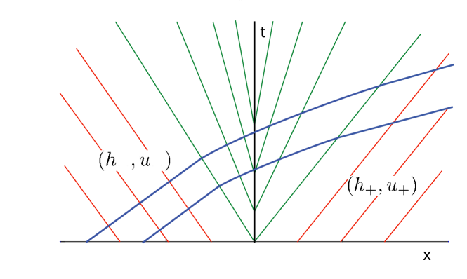
Figure 1: Characteristics in the $(x,t)$-plane for the expansion shock solution of system (1).

In Fig. 1, we show schematically the structure of characteristics for the evolution of the Boussinesq stationary expansion shock suggested by the BBM approximation. The smoothed jump initial data for $h,u$ are indicated as subscripts “$-$” for $-x\gg\delta,$ and “$+$” for $+x\gg\delta$. In the rarefaction wave, the characteristic speed $\lambda_{1}$ is varying, increasing from left to right, and the characteristics have correspondingly different speeds as they emerge from the shock. Moreover, $\lambda_{2}$ is changing also, so the fast characteristics are curved as they pass through the simple wave. But the Riemann invariant $s$ is constant on these characteristics, and therefore, takes the value $s_{-}=s(h_{-},u_{-})$ to the left, and $s_{+}=s(h_{+},u_{+})$ to the right. As we have shown (see (14)), the jump $s_{+}-s_{-}$ across $x=0$ is small for small to moderate water height jumps $\epsilon$. As a consequence, $s$ turns out to be roughly constant across the entire solution except, as we shall see, in the small, $\delta$-wide region within the expansion shock.

4 Expansion shock for the Boussinesq equations

We now proceed with the detailed asymptotic analysis of expansion shocks for the system (17). Similar to [1], we use matched asymptotic expansions. The key to the analytic construction in [1] is the separable structure of the PDE describing the inner solution with the scaled variables $\xi=x/\delta$, $T=\delta t$. Unfortunately, the Boussinesq equations (17) do not admit such a separation of variables with this scaling of $x,t$ and require a somewhat more sophisticated asymptotic analysis to reveal the detailed internal structure of the expansion shock.

We first consider the inner problem, i.e., near the initial smoothed transition. The precise structure of the smoothed Riemann data will be clarified in the analysis below. Our construction will be based on formal expansions in two small parameters: the initial jump in height $\epsilon\sim H-1$ (eq. (13)) and the jump spatial transition width $\delta$, set by the initial conditions. However, as we shall see, the resulting solution also provides an excellent approximation for moderate values of $H-1$.

4.1 Inner Solution: first order approximation

Assuming the spatial scale $\delta$ of the inner solution to be set by the smoothed initial data, we seek a solution to eqs. (17) in the scaled inner variables $\xi=x/\delta$, $\tau=\mu t$, where the parameter $0<\mu\ll 1$ is an inverse timescale for the development of an expansion shock, which is to be determined. With these scalings, equations (17) become

$$\begin{split}\mu r^{(\mathrm{in})}_{\tau}+\frac{1}{4\delta}(3r^{(\mathrm{in})}+s^{(\mathrm{in})})r^{(\mathrm{in})}_{\xi}&=\frac{\mu}{6\delta^{2}}(r^{(\mathrm{in})}_{\xi\xi\tau}+s^{(\mathrm{in})}_{\xi\xi\tau})\\ \mu s^{(\mathrm{in})}_{\tau}+\frac{1}{4\delta}(r^{(\mathrm{in})}+3s^{(\mathrm{in})})s^{(\mathrm{in})}_{\xi}&=\frac{\mu}{6\delta^{2}}(r^{(\mathrm{in})}_{\xi\xi\tau}+s^{(\mathrm{in})}_{\xi\xi\tau}).\end{split}$$ (20)

We wish to find an approximate solution of system (20) that agrees with the initial conditions (12) to some order of accuracy, specifically for $t=\tau=0,$ and $\xi\to\pm\infty.$ For this, we assume that the parameter $\epsilon$ in (13) is small and expand $r^{(\mathrm{in})}$ and $s^{(\mathrm{in})}$ according to

$$\begin{split}r^{(\mathrm{in})}(\xi,\tau)&=r^{(0)}+\epsilon r^{(1)}(\xi,\tau)+\epsilon^{2}r^{(2)}(\xi,\tau)+\cdots,\\ s&=s^{(0)}+\epsilon^{2}s^{(2)}(\xi,\tau)+\cdots,\end{split}$$ (21)

where $r^{(0)}$, $r^{(1)}$, $r^{(2)}$, $s^{(0)}$, and $s^{(2)}$ are $\mathcal{O}(1)$ as $\epsilon\to 0$, $\delta\to 0$, $\mu\to 0$. The parameter $\epsilon$ is proportional to the initial jump in $r$ from eq. (15), and in the expansion for $s$ we have assumed that $s^{(1)}=0,$ which is consistent with the discussion in the previous section, and could be readily deduced by modifying the analysis below.

Inserting expansions (21) into eq. (20), we obtain

$$\begin{split}&\mu\left(\epsilon r^{(1)}_{\tau}+\cdots\right)\\ &+\frac{1}{4\delta}\left(3r^{(0)}+s^{(0)}+3\epsilon r^{(1)}+\epsilon^{2}(3r^{(2)}+s^{(2)})+\cdots\right)(\epsilon r^{(1)}_{\xi}+\epsilon^{2}r^{(2)}_{\xi}+\cdots)\\ &=\frac{\mu}{6\delta^{2}}\left(\epsilon r^{(1)}_{\xi\xi\tau}+\epsilon^{2}(r^{(2)}_{\xi\xi\tau}+s^{(2)}_{\xi\xi\tau})+\cdots\right)\end{split}$$ (22)

and

$$\begin{split}\left(\mu\epsilon^{2}s^{(2)}_{\tau}+\cdots\right)&+\frac{1}{4\delta}\left(r^{(0)}+3s^{(0)}+\cdots\right)(\epsilon^{2}s^{(2)}_{\xi}+\cdots)\\ &=\frac{\mu}{6\delta^{2}}(\epsilon r^{(1)}_{\xi\xi\tau}+\cdots).\end{split}$$ (23)

If we assume $\mu\ll 1/\delta$, then the leading order term in eq. (22) is

$$\mathcal{O}\left(\frac{\epsilon}{\delta}\right):\quad\frac{1}{4}(3r^{(0)}+s^{(0)})r^{(1)}_{\xi}=0,$$ (24)

which is solved by

$$r^{(0)}=-\frac{s^{(0)}}{3}.$$ (25)

In order to find an approximate inner solution that balances nonlinearity and dispersion in eq. (22), we require

$$\mu\epsilon\ll\epsilon^{2}/\delta=\mathcal{O}(\mu\epsilon/\delta^{2}).$$ (26)

This determines the inverse timescale $\mu$ in terms of the transition width $\delta$ and jump amplitude parameter $\epsilon$. We take

$$\mu=\delta\epsilon.$$ (27)

Proceeding under these assumptions, we obtain from eq. (22)

$$\mathcal{O}\left(\frac{\epsilon^{2}}{\delta}\right):\quad r^{(1)}r^{(1)}_{\xi}=\frac{2}{9}r^{(1)}_{\xi\xi\tau}.$$ (28)

We can now solve this equation by separation of variables

$$r^{(1)}(\xi,\tau)=a(\tau)f(\xi)$$ (29)

where

$$\frac{2\dot{a}}{9a^{2}} =\frac{ff^{\prime}}{f^{\prime\prime}}=-K,$$ (30)

and $K>0$ is the separation constant. We determine $a$ and $f$ as for BBM in [1]

$$a(\tau)=\frac{A}{\frac{9}{2}AK\tau+1},\quad f(\xi)=B\tanh\left(\frac{B}{2K}\xi\right),$$ (31)

where $A>0$ and $B>0$ are parameters to be determined. We choose the parameters

$$B=1,\quad K=\frac{1}{2},$$ (32)

and retain the amplitude parameter $A$, which will be determined by the RH locus, so that the solution (31) is

$$a(\tau)=\frac{A}{\frac{9}{4}A\tau+1},\quad f(\xi)=\tanh(\xi).$$ (33)

Then, the approximate inner expansion shock solution to first order in $\epsilon$ can be written

$$r^{(\mathrm{in})}(\xi,\tau) =-\frac{s^{(0)}}{3}+\frac{\epsilon A}{\frac{9}{4}A\tau+1}\tanh(\xi)+\mathcal{O}(\epsilon^{2}),$$ (34)

$$s^{(\mathrm{in})}(\xi,\tau) =s^{(0)}+\mathcal{O}(\epsilon^{2}).$$ (35)

In order to determine the free parameters $s^{(0)}$ and $A$ in terms of the initial data, we evaluate the solution (34), (35) at $t=0$, $\xi\to\pm\infty$ and compare it with the first order small-jump expansions of the initial conditions (12) incorporating the RH locus:

$$r_{\pm} =-\frac{s^{(0)}}{3}\pm\epsilon A+\mathcal{O}(\epsilon^{2}),$$ (36)

$$s_{\pm} =s^{(0)}+\mathcal{O}(\epsilon^{2}),\quad\xi\to\pm\infty.$$ (37)

Comparing eqs. (36) and (37) with eqs. (14) and (15), we find

$$s^{(0)}=3+\frac{3}{4}\epsilon,\quad A=1.$$ (38)

We note that the constructed first order inner solution (34), (35), (38) for the expansion shock simultaneously incorporates the simple wave locus $s_{-}=s_{+}=s^{(0)}$ of the shallow water equations (7) and the RH condition $v_{-}+v_{+}=0$ for the stationary shock of the simple wave equation $v_{t}+vv_{x}=0$, where $v=\tfrac{1}{4}(s^{(0)}+3r)$ (recall eq. (19)). This is nothing but the dispersionless limit of the BBM equation (18). Indeed, one can see that the first order solution written in terms of $v$ agrees with the inner solution for the BBM expansion shock obtained in [1]. We also note that, within the first order approximation, the ordering between the small parameters $\epsilon$ and $\delta$ is $\mu=\delta\epsilon\ll 1/\delta$ or $\epsilon\ll 1/\delta^{2}$.

4.2 Inner solution: second order approximation

To obtain the $\mathcal{O}(\epsilon^{2})$ correction, we consider equation (23), from which we deduce, using $r^{(1)}=a(\tau)f(\xi)$ from the previous subsection,

$$\mathcal{O}\left(\frac{\epsilon^{2}}{\delta}\right):\quad s^{(2)}_{\xi}=\frac{1}{12}r^{(1)}_{\xi\xi\tau}=\frac{1}{12}\dot{a}(\tau)f^{\prime\prime}(\xi).$$ (39)

This equation is solved with

$$s^{(2)}(\xi,\tau)=\frac{1}{12}\dot{a}(\tau)f^{\prime}(\xi)+C=-\frac{3\,\mathrm{sech}^{2}(\xi)}{16\left(1+\frac{9}{4}\tau\right)^{2}}+C.$$ (40)

The constant of integration $C$ could at this stage be a function of $\tau,$ but it will be determined below by matching to the far field, so it is necessarily constant.

We now proceed to the next order equation in (22), assuming that $\delta\epsilon^{2}\ll\epsilon^{3}/\delta$, implying the basic small parameter ordering

$$\delta\ll\epsilon^{1/2}.$$ (41)

We find the equation for $r^{(2)}:$

$$\mathcal{O}\left(\frac{\epsilon^{3}}{\delta}\right):\quad r^{(2)}_{\xi\xi\tau}-\frac{9}{2}(r^{(1)}r^{(2)})_{\xi}=\frac{3}{2}s^{(2)}r^{(1)}_{\xi}-s^{(2)}_{\xi\xi\tau}.$$ (42)

We observe that this equation has solutions of the form

$$r^{(2)}(\xi,\tau)=a^{2}(\tau)g(\xi)-\frac{C}{3},$$ (43)

in which $a(\tau)$ is given in (33). Then $g$ satisfies

$$g^{\prime\prime}+(fg)^{\prime}=\frac{1}{16}\left(f^{\prime 2}+3f^{\prime\prime\prime}\right)=\frac{1}{16}\left(f^{\prime}-f^{\prime}f^{2}+3f^{\prime\prime\prime}\right).$$ (44)

Integrating, we obtain

$$g^{\prime}+fg=\frac{1}{16}\left(f-\frac{1}{3}f^{3}+3f^{\prime\prime}+\frac{1}{3}D\right),$$ (45)

where $D$ is a constant of integration. An integrating factor for this equation is $\mathrm{cosh}(\xi)$. We therefore obtain

$$g(\xi)=\frac{1}{16}\left(\frac{2}{3}+\frac{17}{3}\,\mathrm{sech}^{2}(\xi)+\frac{1}{3}D\tanh(\xi)+\frac{1}{3}E\,\mathrm{sech}(\xi)\right),$$ (46)

where $E$ is an additional constant of integration. Then the approximate inner solution for the expansion shock to second order in $\epsilon$ becomes

$$\begin{split}r^{(\mathrm{in})}(\xi,\tau)&\sim-1+\epsilon\left(-\frac{1}{4}+\frac{\tanh(\xi)}{1+\frac{9}{4}\tau}\right)\\ &\qquad~{}~{}+\frac{\epsilon^{2}}{3}\left(-C+\frac{2+17\,\mathrm{sech}^{2}(\xi)+D\tanh(\xi)+E\,\mathrm{sech}(\xi)}{16\left(1+\frac{9}{4}\tau\right)^{2}}\right),\\ s^{(\mathrm{in})}(\xi,\tau)&\sim 3+\frac{3}{4}\epsilon+\epsilon^{2}\left(C-\frac{3\,\mathrm{sech}^{2}(\xi)}{16\left(1+\frac{9}{4}\tau\right)^{2}}\right).\end{split}$$ (47)

The constant $E$ is a free parameter, not determined at this order. We therefore set $E=0$. To determine the remaining parameters $C$ and $D$, we invoke the smoothed Riemann data (12) and evaluate the approximate solution (47) at $t=0$ for $r^{(\mathrm{in})}$ and $s^{(\mathrm{in})}$ as $\xi\to\pm\infty$, yielding (cf. (36), (37)),

$$\begin{split}r_{\pm}&=-1+\epsilon\left(-\frac{1}{4}\pm 1\right)+\epsilon^{2}\left(-\frac{C}{3}+\frac{1}{24}\pm\frac{D}{48}\right)+\mathcal{O}(\epsilon^{3}),\\ s_{\pm}&=3+\frac{3}{4}\epsilon+C\epsilon^{2}+\mathcal{O}(\epsilon^{3}),\end{split}$$ (48)

which satisfy the RH locus expansions (14) and (15) to $\mathcal{O}(\epsilon^{2})$ if we take

$$C=\frac{1}{32},\quad D=0,$$ (49)

which, together with (47), fully defines the second order inner solution, beyond the BBM approximation as

$$\begin{split}r^{(\mathrm{in})}(\xi,\tau)&\sim-1+\epsilon\left(-\frac{1}{4}+\frac{\tanh(\xi)}{1+\frac{9}{4}\tau}\right)+\frac{\epsilon^{2}}{48}\left(-\frac{1}{2}+\frac{2+17\,\mathrm{sech}^{2}(\xi)}{\left(1+\frac{9}{4}\tau\right)^{2}}\right),\\ s^{(\mathrm{in})}(\xi,\tau)&\sim 3+\frac{3}{4}\epsilon+\frac{\epsilon^{2}}{16}\left(\frac{1}{2}-\frac{3\,\mathrm{sech}^{2}(\xi)}{\left(1+\frac{9}{4}\tau\right)^{2}}\right).\end{split}$$ (50)

4.3 Outer Solution

For matching purposes, it is natural to set the timescale for the outer scaling to be the same as the timescale of the inner scaling $\tau=\mu t=\delta\epsilon t$, using (27). Along with that, we use the long wave, hydrodynamic scaling $X=\delta x$, which is independent of the jump amplitude parameter $\epsilon$. Then the leading order (in $\delta$) equations from (17) are the dispersionless shallow water equations

$$\begin{split}\epsilon r^{(\mathrm{out})}_{\tau}+\frac{1}{4}(3r^{(\mathrm{out})}+s^{(\mathrm{out})})r^{(\mathrm{out})}_{X}&=0,\\ \epsilon s^{(\mathrm{out})}_{\tau}+\frac{1}{4}(r^{(\mathrm{out})}+3s^{(\mathrm{out})})s^{(\mathrm{out})}_{X}&=0.\end{split}$$ (51)

We expect a simple wave solution, which we expand as

$$\begin{split}s^{(\mathrm{out})}(X,\tau)&=3+\frac{3}{4}\epsilon+\frac{1}{32}\epsilon^{2}+\cdots,\\ r^{(\mathrm{out})}(X,\tau)&=-1+\epsilon\left(-\frac{1}{4}+r_{1}(X,\tau)\right)+\epsilon^{2}\left(-\frac{1}{96}+r_{2}(X,\tau)\right)+\cdots.\end{split}$$ (52)

With these expansions, the equation (51) for $s^{(\mathrm{out})}$ is identically satisfied. The equation for $r^{(\mathrm{out})}$, expanded in powers of $\epsilon$, yields to leading order

$$\mathcal{O}(\epsilon^{2}):\quad r_{1,\tau}+\frac{3}{4}r_{1}r_{1,X}=0,$$ (53)

which can be solved with

$$r_{1}(X,\tau)=F_{1}^{(\mathrm{sgn}\,X)}\left(\tau-\frac{4X}{3r_{1}}\right),$$ (54)

where we use the functions $F_{1}^{(\pm)}$ depending on whether $\pm X>0$. Matching this to the inner solution (50) at $\mathcal{O}(\epsilon)$ yields

$$\lim_{X\to 0^{\pm}}r_{1}(X,\tau)=F_{1}^{(\pm)}(\tau)=\lim_{\xi\to\pm\infty}r^{(1)}(\xi,\tau)=\pm\frac{1}{1+\frac{9}{4}\tau}$$ (55)

Then

$$r_{1}=\frac{\mathrm{sgn}\,X}{1+\frac{9}{4}\tau-\frac{3X}{r_{1}}},$$ (56)

which is solved by

$$r_{1}(X,\tau)=\frac{\mathrm{sgn}\,X+3X}{1+\frac{9}{4}\tau}.$$ (57)

Proceeding to the next order in the expansion of eq. (51) yields an equation for $r_{2}$

$$\mathcal{O}(\epsilon^{3}):\quad r_{2,\tau}+\frac{3}{4}(r_{1}r_{2})_{X}=0.$$ (58)

One can verify by direct substitution that

$$r_{2}(X,\tau)=F_{2}^{(\mathrm{sgn}\,X)}\frac{1+3|X|}{\left(1+\frac{9}{4}\tau\right)^{2}},$$ (59)

solves eq. (58). Matching to the inner solution (50), we obtain

$$\lim_{X\to 0^{\pm}}r_{2}(X,\tau)=F_{2}^{\pm}\frac{1}{\left(1+\frac{9}{4}\tau\right)^{2}}=\lim_{\xi\to\pm\infty}r^{(2)}(\xi,\tau)=\frac{1}{24\left(1+\frac{9}{4}\tau\right)^{2}},$$ (60)

so that $F_{2}^{+}=F_{2}^{-}=1/24$, yielding the second order correction to the outer solution

$$r_{2}(X,\tau)=\frac{1+3|X|}{24\left(1+\frac{9}{4}\tau\right)^{2}}.$$ (61)

The approximate outer solution therefore has the form

$$\begin{split}r^{(\mathrm{out})}(X,\tau)&=-1+\epsilon\left(-\frac{1}{4}+\frac{\mathrm{sgn}\,X+3X}{1+\frac{9}{4}\tau}\right)\\ &\quad\,+\frac{\epsilon^{2}}{24}\left(-\frac{1}{4}+\frac{1+3|X|}{\left(1+\frac{9}{4}\tau\right)^{2}}\right)+\mathcal{O}(\epsilon^{3}),\\ s^{(\mathrm{out})}(X,\tau)&=3+\frac{3}{4}\epsilon+\frac{1}{32}\epsilon^{2}+\mathcal{O}(\epsilon^{3}).\end{split}$$ (62)

Note that for the dispersionless eq. (51) to be a valid asymptotic approximation of the full Boussinesq eqs. (17) to $\mathcal{O}(\epsilon^{3})$, we require the dispersive term to be negligible to the order considered, i.e., $\epsilon\delta^{3}\ll\epsilon^{3}$ or $\delta\ll\epsilon^{2/3}$. This is a less stringent condition on scale separation than the restriction (41) applied for the calculation of the inner solution.

This approximate outer solution is only valid within an expanding region. We invoke continuous matching to the far-field along the two lines

$$X=c_{\pm}\tau,$$ (63)

where $c_{\pm}$ is determined by the requirement

$$r^{(\mathrm{out})}(c_{\pm}\tau,\tau)=r_{\pm}.$$ (64)

A calculation using (15), (62) yields the speeds

$$c_{\pm}=\pm\frac{3}{4}+\frac{1}{32}\epsilon+\cdots.$$ (65)

Matching to the far-field, we obtain the approximate, piecewise smooth outer solution

$$\begin{split}\scriptstyle r^{(\mathrm{out})}(X,\tau)&=\scriptstyle-1+\epsilon\begin{cases}\textstyle-\frac{5}{4}+\frac{1}{32}\epsilon&\scriptstyle\frac{X}{\tau}\leq c_{-},\\[8.53581pt] \textstyle-\frac{1}{4}+\frac{\mathrm{sgn}\,X+3X}{1+\frac{9}{4}\tau}+\frac{\epsilon}{24}\left(-\frac{1}{4}+\frac{1+3|X|}{\left(1+\frac{9}{4}\tau\right)^{2}}\right)&\scriptstyle c_{-}<\frac{X}{\tau}<c_{+},\\[8.53581pt] \textstyle\frac{3}{4}+\frac{1}{32}\epsilon&\scriptstyle c_{+}\leq\frac{X}{\tau},\end{cases}+\mathcal{O}(\epsilon^{3}),\\ s^{(\mathrm{out})}(X,\tau)&=3+\frac{3}{4}\epsilon+\frac{1}{32}\epsilon^{2}+\mathcal{O}(\epsilon^{3}).\end{split}$$ (66)

4.4 Uniformly Valid Asymptotic Solution

In order to construct a uniformly valid (in $x$) asymptotic solution to $\mathcal{O}(\epsilon^{2})$ in $r$ and $s$, we introduce the composite solution

$$\begin{array}[]{rcl}r(x,t)&=&r^{(\mathrm{in})}(x/\delta,\delta\epsilon t)+r^{(\mathrm{out})}(\delta x,\delta\epsilon t)-r^{(\mathrm{overlap})}(x,t;\delta,\epsilon),\\ s(x,t)&=&s^{(\mathrm{in})}(x/\delta,\delta\epsilon t)+s^{(\mathrm{out})}(\delta x,\delta\epsilon t)-s^{(\mathrm{overlap})}(x,t;\delta,\epsilon).\end{array}$$ (67)

We subtract the “overlap” portion (common to both the inner and outer solutions) so that we do not double count the matching region. We therefore have

$$\begin{split}r^{(\mathrm{overlap})}(x,t;\delta,\epsilon)&\sim-1+\epsilon\left(-\frac{1}{4}+\frac{\mathrm{sgn}\,X}{1+\frac{9}{4}\tau}\right)+\frac{\epsilon^{2}}{24}\left(-\frac{1}{4}+\frac{1}{\left(1+\frac{9}{4}\tau\right)^{2}}\right),\\ s^{(\mathrm{overlap})}(x,t;\delta,\epsilon)&\sim 3+\frac{3}{4}\epsilon+\frac{1}{32}\epsilon^{2}.\end{split}$$ (68)

Then the uniformly valid, composite asymptotic solution for an expansion shock is

$$\begin{split}r(x,t;\delta,\epsilon)&\sim-1+\epsilon\left(\frac{\tanh\left(\frac{x}{\delta}\right)-\,\mathrm{sgn}\,(x)}{1+\frac{9}{4}\delta\epsilon t}+G_{1}(x,t;\delta,\epsilon)\right)\\ &\qquad+\epsilon^{2}\left(\frac{17\,\mathrm{sech}^{2}\left(\frac{x}{\delta}\right)}{48\left(1+\frac{9}{4}\delta\epsilon t\right)^{2}}+G_{2}(x,t;\delta,\epsilon)\right),\\[8.53581pt] s(x,t)&\sim 3+\frac{3}{4}\epsilon+\frac{\epsilon^{2}}{16}\left(\frac{1}{2}-\frac{3\,\mathrm{sech}^{2}\left(\frac{x}{\delta}\right)}{\left(1+\frac{9}{4}\delta\epsilon t\right)^{2}}\right),\\[8.53581pt] G_{1}(x,t;\delta,\epsilon)&=\begin{cases}\displaystyle-\frac{5}{4}&\displaystyle\frac{x}{\epsilon t}\leq c_{-},\\[8.53581pt] \displaystyle-\frac{1}{4}+\frac{\mathrm{sgn}\,(x)+3\delta x}{1+\frac{9}{4}\delta\epsilon t}&\displaystyle c_{-}<\frac{x}{\epsilon t}<c_{+},\\[8.53581pt] \displaystyle\frac{3}{4}&\displaystyle c_{+}\leq\frac{x}{\epsilon t},\end{cases}\\[8.53581pt] G_{2}(x,t;\delta,\epsilon)&=\begin{cases}\displaystyle\frac{1}{32}&\displaystyle\frac{x}{\epsilon t}\leq c_{-},\\[8.53581pt] \displaystyle-\frac{1}{96}+\frac{1+3\delta|x|}{24\left(1+\frac{9}{4}\delta\epsilon t\right)^{2}}&\displaystyle c_{-}<\frac{x}{\epsilon t}<c_{+},\\[8.53581pt] \displaystyle\frac{1}{32}&\displaystyle c_{+}\leq\frac{x}{\epsilon t},\end{cases}\end{split}$$ (69)

where $c_{\pm}$ is given in (65). This solution can be used in (6) to reconstruct the expansion shock water height $h$ and horizontal velocity $u$.

5 Numerical Simulation

We validate the asymptotic analysis of §4.4 with direct numerical simulations of the Boussinesq equations (1) with initial data consisting of the approximate expansion shock solution (69) evaluated at $t=0$. The numerical method is described in the appendix.

Figure 2 depicts the numerical evolution of $h$ and $u$ with an initial jump in $h$ from unity to $H=1.4$ and the transition width $\delta=0.1$. The boundary conditions $u_{\pm}$, determined by eqs. (8), (14), and (15), satisfy the RH locus (4) to order $\epsilon^{2}$. The sharp initial step evolves into an expansion shock that algebraically decays between non-centered rarefaction waves propagating left and right. The uniform asymptotic approximation (69) closely follows the numerical solution; the most noticeable deviations occurring at the weak discontinuities, where the rarefactions meet the far-field boundary conditions with a jump in the first derivative of the asymptotic solution. A close examination reveals the generation of a small amplitude dispersive wavepacket that propagates to the right (see insets at $t=15$). This is due to the fact that the initial data only approximately corresponds to an expansion shock, accurate to order $\epsilon^{2}$. For this simulation, $\epsilon=2(\sqrt{H}-1)\approx 0.366,$ for which $\epsilon^{3}\sim 0.05,$ larger than the size of the dispersive wavepacket.

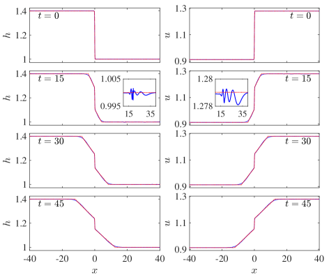
Figure 2: Numerical simulation of the Boussinesq equation for expansion shock initial data in physical variables $h$, $u$ (solid) compared with the the uniform asymptotic approximation (dotted) for $H=1.4$, $\epsilon\approx 0.366$, $\delta=0.1$.

It is revealing to examine the evolution of the scaled Riemann variables $r$ and $s$ in Fig. 3. The variable $r$ evolves much like $h$ and $u$, with order one changes in amplitude. The smooth, decaying expansion shock structure is accurately resolved by the asymptotic approximation, as shown in the insets. The evolution of $s$, on the other hand, is at a much smaller amplitude scale. Recall that the RH locus (4) leads to an order $\epsilon^{3}$ jump in $s$ across an expansion shock. This variation in $s$ is not captured by our asymptotic approximation (69) and is the source of the dispersive wavepacket that propagates away from the initial transition. Note that although the oscillations appear sharp in the figure, they are smoothly and accurately resolved by the numerical simulation. Presumably, a higher order correction to the obtained expansion shock approximation (69) would reduce the amplitude of this wavepacket. Nevertheless, the initial, order $\epsilon^{2}$ amplitude dip in $s$ at the transition is apparent and accurately captured by the asymptotic approximation.

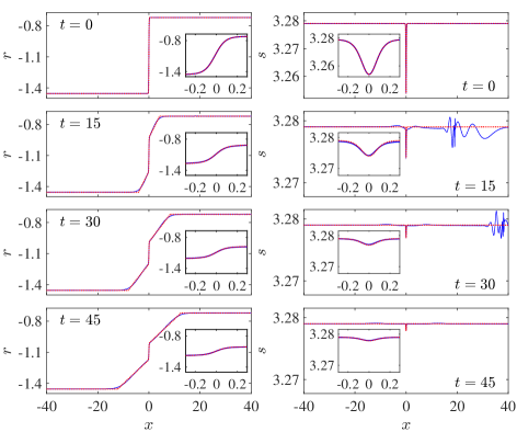
Figure 3: Numerical simulation of the Boussinesq equation for expansion shock initial data in the transformed variables $r$, $s$ (solid) compared with the uniform asymptotic approximation (dotted) for $H=1.4$, $\epsilon\approx 0.366$, $\delta=0.1$. The insets reveal the zoomed in expansion shock structure. Note the change in the $s$ amplitude scale for $t>0$.

We undertake an error analysis of the asymptotic expansion shock solution (69) by performing numerical simulations with variable initial jump height parameter $\epsilon$ and fixed transition width $\delta=0.1$. Figure 4 shows a summary of the results, comparing the infinity norm difference between the asymptotic approximation, denoted by the subscript “a”, and the numerical solution for both $h$ and $s$ as $\epsilon$ is varied. The errors in $u$ and $r$ are similar to those for $h$. The norm difference is computed across the entire simulation domain, i.e., for $x\in[-L,L]$ and $t\in[0,T]$. For these simulations $L=120$, $T=45$. Both $h$ and $s$ show an approximately $\mathcal{O}(\epsilon^{5/2})$ dependence of the error over a portion or all of the jump heights considered. The dominant contribution to these errors is due to the dispersive wavepacket that is generated by the discrepancy in the approximate initial data (recall the insets in Fig. 2). The error is consistent with the formal second order accuracy of the asymptotic solution. It is striking that the asymptotic solution exhibits small error, even for values of $\epsilon$ above one. Below $\epsilon=0.6$, the error in $h$ decays at a slower rate approximately proportional to $\epsilon$. This is because the dominant error contribution now comes from the region where the non-centered rarefaction waves are matched to the constant background, eq. (64). The higher order approximation fails to resolve this region, which is smoothed in the numerical solution by dispersion. This discrepancy is visible in Fig. 2.

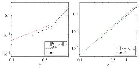
Figure 4: Error analysis of approximate expansion shock solution for variable $\epsilon$ and fixed $\delta=0.1$. We compare simulations of the Boussinesq equations with the asymptotic solution (69) in the infinity norm for $h$ (left) and $s$ (right).

6 Discussion

Decaying expansion shocks were recently identified as robust solutions to conservation laws of non-evolutionary type that naturally arise in shallow water theory. In [1] we studied these shocks in the framework of the unidirectional BBM equation, using matched asymptotic expansions. In the present paper, the analysis of [1] is extended to a bi-directional regularized Boussinesq system [2]. The extension to the bi-directional case is more complicated, and has revealed further structure of expansion shocks exhibiting subtle but essential features that appear in the second order corrections of the matched asymptotic expansion, while the first order solution is equivalent to the BBM expansion shock. The key feature of our analysis of the Boussinesq expansion shocks is the use of the Riemann invariants of the underlying ideal shallow water equations as field variables in the full dispersive system. Another important feature is the requirement of the balance between two small parameters: the width $\delta$ of the smoothed Riemann data satisfying the stationary expansion shock Rankine-Hugoniot conditions and the value of the initial jump of the water height, measured by $\epsilon$. The product $\mu=\epsilon\delta$ then sets the inverse time scale for the algebraic decay of the expansion shock.

A natural extension of this work is the consideration of jump initial data that does not lie on the RH locus (4). An analogous problem was numerically studied in the context of the BBM equation (18) corresponding to asymmetric, positive jump initial data passing through $v=0$ [1]. There, an expansion shock forms accompanied by a sequence of solitary waves, the number depending upon the asymmetry of the data. The bi-directional nature of the Boussinesq equations (1) suggests a richer set of outcomes.

The comparison of the obtained second order asymptotic formula with accurate numerical solution of the smoothed Riemann problem for the Boussinesq system reveals remarkable agreement, even for relatively large initial jumps, beyond the formal applicability of our asymptotic analysis. In conclusion, we note that, in considering more general initial data, the use of the “dispersionless” Riemann invariants as dependent variables in the full system may give insight into the structure of solutions, since the interaction between the two fields occurs primarily through the dispersive terms, except where waves collide.

Appendix

A pseudospectral Fourier spatial discretization with standard fourth order Runge-Kutta timestepping is utilized. We discretize the domain $[-L,L]$ according to $x_{n}=-L+2Ln/N$, $n=0,\cdots,N-1$. In order to accommodate non-periodic boundary conditions in $h$ and $u$, the spatial derivatives $g=h_{x}$, $v=u_{x}$ are numerically evolved according to

$$\begin{split}g_{t}+(ug)_{x}+(hv)_{x}&=0,\\ v_{t}+(uv)_{x}+g_{x}-\frac{1}{3}v_{xxt}&=0.\end{split}$$ (70)

By choosing a sufficiently large domain $L$, the boundary quantities $|h(\pm L,t)-h_{\pm}|$ and $|u(\pm L,t)-u_{\pm}|$ are maintained to within $10^{-9}$ for the duration of the simulation, therefore $g$ and $v$ can be treated as localized, periodic functions. Each un-differentiated term in eq. (70) is spatially localized, therefore we can compute their derivatives in spectral space, e.g.,

$$\mathcal{F}\{(ug)_{x}\}_{n}=ik_{n}\mathcal{F}\{ug\}_{n},\quad n=-N/2,\cdots,N/2-1,$$ (71)

where $\mathcal{F}$ is the discrete, finite Fourier series operator, efficiently implemented via the FFT, and $k_{n}=n\pi/L$ are the discrete wavenumbers. The function $h$ is approximated by an accumulation of its derivative $g$ according to

$$h(x_{n},t)=h_{-}+\mathcal{F}^{-1}\left\{\tilde{g}(t)\right\}_{n}+\frac{1}{2L}(h_{+}-h_{-})(x_{n}+L),$$ (72)

where

$$\tilde{g}_{n}(t)=\begin{cases}\displaystyle-\sum_{m=-N/2}^{N/2-1}x_{m}g(x_{m},t)&n=0\\[17.07164pt] \displaystyle\frac{\hat{g}_{n}(t)}{ik_{n}}&n\neq 0\end{cases}.$$ (73)

The sum for $n=0$ in (73) is a trapezoidal approximation of the integral $\int_{-L}^{L}xg(x,t)dx$ so that an accurate, efficient reconstruction of $h$ from $g$ is achieved. A similar computation is performed to obtain $u$.

Time evolution is performed on the spectral, Fourier coefficients using the standard fourth order Runge-Kutta method. The nonlocal character of the dispersive term $v_{xxt}/3$ in eq. (70) is not stiff so we use a timestep of $0.002$ and evolve to $t=45$. The domain size is $L=120$ (Figures 2 and 3 show only a portion of the domain) and the Fourier truncation is $N=2^{14}$. The accuracy of the numerical computation is monitored by ensuring that the conserved quantities $|\int_{-L}^{L}g(x,t)dx-h_{+}+h_{-}|$, $|\int_{-L}^{L}v(x,t)dx-u_{+}+u_{-}|$ are maintained to less than $10^{-14}$ and the Fourier components $|\mathcal{F}\{g\}_{n}|$, $|\mathcal{F}\{v\}_{n}|$, $n=-N/2,\ldots,N/2-1$ decay to about $10^{-8}$, within the expected value given boundary deviations of about $10^{-9}$.

References

- [1] G. A. El, M.A. Hoefer and M. Shearer, Expansion shock waves in regularized shallow water theory. Proc. Roy. Soc. London 472: 20160141 (2016)
- [2] G. B. Whitham, Linear and Nonlinear Waves. (Wiley, New York, 1974).
- [3] J. L. Bona, M. Chen and J. C. Saut, Boussinesq equations and other systems for small–amplitude long waves in nonlinear dispersive media. I: derivation and linear theory. J Nonlinear Sci. 12: 283-318 (2002).
- [4] G. A. El and M.A. Hoefer, Dispersive shock waves and modulation theory, Physica D 33: 11-65 (2016).
- [5] G. A. El, M.A. Hoefer and M. Shearer, Dispersive and diffusive-dispersive shock waves for non-convex conservation laws, SIAM Review (2017), accepted
- [6] P. D. Lax, Hyperbolic Systems of Conservation Laws II, Comm. Pure Appl. Math. 10: 537-566 (1957).
- [7] A. Bressan, Hyperbolic Systems of Conservation Laws: The One-Dimensional Cauchy Problem. (Oxford Univ. Press, 2000).
- [8] F. Dias and P. Milewski, On the fully-nonlinear shallow-water generalized Serre equations, Phys. Lett. A 374: 1049-1053 (2010).