On convergence rates of game theoretic reinforcement learning algorithms

Abstract

This paper investigates a class of multi-player discrete games where each player aims to maximize its own utility function. Each player does not know the other players’ action sets, their deployed actions or the structures of its own or the others’ utility functions. Instead, each player only knows its own deployed actions and its received utility values in recent history. We propose a reinforcement learning algorithm which converges to the set of action profiles which have maximal stochastic potential with probability one. Furthermore, the convergence rate of the proposed algorithm is quantified. The algorithm performance is verified using two case studies in the smart grid and cybersecurity.

AND

, , ,

1 Introduction

Game theory provides a mathematically rigorous framework for multiple players to reason about each other. In recent years, game theoretic learning has been increasingly used to control large-scale networked systems due to its inherent distributed nature. In particular, the network-wide objective of interest is encoded as a game whose Nash equilibria correspond to desired network-wide configurations. Numerical algorithms are then synthesized for the players to identify Nash equilibria via repeated interactions. Multi-player games can be categorized into discrete games and continuous games. In a discrete (resp. continuous) game, each player has a finite (resp. an infinite) number of action candidates. As for discrete games, learning algorithms include best-response dynamics, better-response dynamics, factitious play, regret matching, logit-based dynamics and replicator dynamics. Please refer to (Basar and Olsder, 1999; Fudenberg and Levine, 1998; Sandholm, 2010; Young, 2001) for detailed discussion. As an important class of continuous games, generalized Nash games were first formulated in Arrow and Debreu (1954), and see survey paper Facchinei and Kanzow (2007) for a comprehensive exposition. A number of algorithms have been proposed to compute generalized Nash equilibria, including, to name a few, ODE-based methods Rosen (1965), nonlinear Gauss-Seidel-type approaches Pang et al. (2008), iterative primal-dual Tikhonov schemes Yin et al. (2011), and best-response dynamics Palomar and Eldar (2010). Game theory and its learning have found many applications; e.g., traffic routing in Internet Altman et al. (2002), urban transportation Roumboutsos and Kapros (2008), mobile robot coordination (Arslan et al., 2007; Hatanaka et al., 2016) and power markets (Wang et al., 2012; Zhu, 2014).

In many applications, players can only access limited information about the game of interest. For example, each player may not know the structure of its own utility function. Additionally, during repeated interactions, each player may not be aware of the actions of other players. These informational constraints motivate recent study on payoff-based or reinforcement learning algorithms where the players adjust their actions only based on their own previous actions and utility measurements. The papers (Marden et al., 2009; Zhu and Martínez, 2013; Hatanaka et al., 2016) study discrete games, and their approaches are based on stochastic stability Foster and Young (1990). As mentioned in Remark 3.2 of Zhu and Martínez (2013), paper Marden et al. (2009) proposes an algorithm to find Nash equilibrium of weakly acyclic games with an arbitrarily high probability by choosing an arbitrarily small and fixed exploration rate in advance. The analysis in Marden et al. (2009) is based on homogeneous Markov chains and more specifically the theory of resistance trees Young (1993). Zhu and Martínez (2013) extends the results in Marden et al. (2009) by adopting diminishing exploration rates and ensures convergence to Nash equilibrium and global optima with probability one. The analysis of Zhu and Martínez (2013) is based on based on strong ergodicity of inhomogeneous Markov chains. As for continuous games, the papers (Frihauf et al., 2012; Liu and Krstic, 2011; Stankovic et al., 2012) employ extremum seeking and the paper Zhu and Frazzoli (2016) uses finite-difference approximations to estimate unknown partial (sub)gradients. Notice that all the aforementioned papers focus on asymptotic convergence and none of them quantifies convergence rates.

Contribution: In this paper, we study a class of multi-player discrete games where each player is unaware of the other players’ action sets, their deployed actions or the structures of its own or the others’ utility functions. We propose a reinforcement learning algorithm where, at each iteration, each player, on one hand, exploits successful actions in recent history via comparing received utility values, and on the other hand, randomly explores any feasible action with a certain exploration rate. The algorithm is proven to be convergent to the set of action profiles with maximum stochastic potential with probability one. Furthermore, an upper bound on the convergence rate is derived and is minimized when the exploration rates are restricted to $\mathbf{p}$-series. When the interactions of the players consist of a weakly acyclic game and the received utilities are subject to uniformly bounded random noises, the convergence to the set of pure anti-$\mathcal{E}$-Nash equilibria is guaranteed. The algorithm performance is verified using two case studies in the smart grid and cybersecurity. A preliminary version of this paper was published in Zhu et al. (2014) where convergence rates and measurement noises are not discussed. Further, Zhu et al. (2014) focuses on the application on adaptive cyber defense, and this paper focuses on theory of learning in games. The analysis of two papers is significantly different.

2 Problem formulation and learning algorithm

In this section, we introduce a class of multi-player games where the information each player accesses is limited. Then, we present a learning algorithm under which the action profiles of the players converge to the set of action profiles which have maximum stochastic potential.

2.1 Game formulation

The system model in Figure 1 characterizes the interactions of $N$ players in a non-cooperative game. Each component in the figure will be discussed in the following paragraphs.

Figure 1: Game model

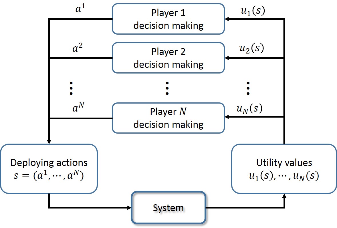
Players. We consider $N$ players $\mathcal{V}\triangleq\{1,\cdots,N\}$ and each player has a finite set of actions. Let $\mathcal{A}_{i}$ denote the action set of player $i$ and $a^{i}\in\mathcal{A}_{i}$ denote an action of player $i$. Denote $\mathcal{S}\triangleq\mathcal{A}_{1}\times\cdots\times\mathcal{A}_{N}$ as the Cartesian product of the action sets, where $s\triangleq(a^{1},\cdots,a^{N})\in\mathcal{S}$ is denoted as an action profile of the players.

Utility. Under the influence of an action profile, the system generates a utility value for each player. The utility function for player $i\in\mathcal{V}$ is defined as $u_{i}:\mathcal{S}\to\mathbb{R}$. At the end of iteration $t$, the utility value $u_{i}(t)=u_{i}(s(t))$ is measured and sent to player $i$. The utility value received by player $i$ is denoted by $\tilde{u}_{i}(t)\triangleq u_{i}(t)+w_{i}(t)$, where $w_{i}(t)$ is the measurement noise.

Informational constraint. Each player does not know the other players’ action sets or their deployed actions. Besides, each player is unaware of the structure of its own or the others’ utility functions. At iteration $t$, each player only knows its deployed actions and its received utility values in the past; i.e., $a^{i}(0),\cdots,a^{i}(t-1),\tilde{u}_{i}(0),\cdots,\tilde{u}_{i}(t-1)$.

The above informational constraint has been studied in several recent papers. For example, the authors in (Zhu and Martínez, 2013; Stankovic et al., 2012; Hatanaka et al., 2016) investigate coverage optimization problems for mobile sensor networks where mobile sensors are unaware of environmental distribution functions. The authors in Marden et al. (2013) study the problem of optimizing energy production in wind farms where each turbine knows neither the functional form of the power generated by the wind farm nor the choices of other turbines. The authors in (Frihauf et al., 2012; Zhu and Frazzoli, 2016) consider convex games where each player cannot access its game components.

2.2 Problem statement

Under the above informational constraint, we aim to synthesize a learning algorithm under which the action profiles of the players converge to the set of action profiles with maximum stochastic potential. We will quantify the convergence rate of the proposed algorithm in contrast to asymptotic convergence in existing work.

2.3 Learning algorithm

Inspired by Zhu and Martínez (2013), we propose a learning algorithm called the RL algorithm, where each player updates its actions only based on its previous actions and its received utility values. On the one hand, each player chooses the most successful action in recent history. It represents the exploitation phase. However, the exploitation is not sufficient to guarantee that the player can choose the best action given others’. So on the other hand, the player uniformly chooses one action from its action set. It represents the exploration phase. The specific update rule is stated in the RL algorithm. At iterations $t=0$ and $t=1$, each player uniformly chooses one action from its action set as initialization (Line 3). Starting from iteration $t=2$, with probability $1-\tilde{\epsilon}_{i}(t)$, player $i$ chooses the action which generates a higher utility value in last two iterations as current action (Line 8-13). This represents the exploitation where player $i$ reinforces its previous successful actions. With probability $\tilde{\epsilon}_{i}(t)$, player $i$ uniformly selects an action from its action set $\mathcal{A}_{i}$ (Line 14). This represents the exploration and makes sure that each action profile is selected infinitely often. Note that ${\rm sample}(\mathcal{A}_{i})$ in Line 14 represents uniformly choosing one element from set $\mathcal{A}_{i}$.

[h]Reinforcement learning (RL) algorithm

1:  while $0\leq t\leq 1$ do

2:     for $i\in\mathcal{V}$ do

3:         $a^{i}(t)\leftarrow{\rm sample}(\mathcal{A}_{i})$;

4:     end for

5:  end while

6:  while $t\geq 2$ do

7:     for $i\in\mathcal{V}$ do

8:        With prob. $(1-\tilde{\epsilon}_{i}(t))$,

9:        if $\tilde{u}_{i}(t-1)\geq\tilde{u}_{i}(t-2)$ then

10:           $a^{i}(t)=a^{i}(t-1)$;

11:        else

12:           $a^{i}(t)=a^{i}(t-2)$;

13:        end if

14:        With prob. $\tilde{\epsilon}_{i}(t)$, $a^{i}(t)\leftarrow{\rm sample}(\mathcal{A}_{i})$;

15:     end for

16:  end while

3 Analysis

In this section, we will present the analytical results of the RL algorithm.

3.1 Notations and assumptions

We first introduce the notations and assumptions used throughout the paper. Denote by $|\mathcal{V}|$ the cardinality of player set, $|\mathcal{A}_{i}|$ the cardinality of action set of player $i$ and $|\mathcal{A}|_{\infty}\triangleq\max\limits_{i\in\mathcal{V}}|\mathcal{A}_{i}|$ the maximum cardinality among all action sets. The exploration rate for player $i$ at iteration $t$ is decomposed into two parts; i.e., $\tilde{\epsilon}_{i}(t)\triangleq\epsilon_{i}(t)+{e_{i}}(t)$, where $\epsilon_{i}(t)=\gamma_{i}{\epsilon}^{c}(t)$, $\gamma_{i}>0$, ${\epsilon}^{c}(t)$ is common for all the players and ${e_{i}}(t)$ represents the exploration deviation. Define $e(t)\triangleq({e_{1}}(t),\cdots,{e_{N}}(t))^{T}$, $\tilde{\epsilon}(t)\triangleq(\tilde{\epsilon}_{1}(t),\cdots,\tilde{\epsilon}_{N}(t))^{T}$ and ${\epsilon}(t)\triangleq(\epsilon_{1}(t),\cdots,\epsilon_{N}(t))^{T}$. And we define $e_{r}(t)\triangleq||{e}(t)||_{\infty}^{N}/\prod\limits_{i=1}^{N}\tilde{\epsilon}_{i}(t)$. Here we denote by $||\cdot||_{\infty}$ the infinity norm of a vector. In addition, we also use $||\cdot||$ to represent the $L^{1}$-norm of a vector, and $||P||$ to represent the 1-norm of a matrix. We assume the measurement noises satisfy:

Assumption 1.

For each $i\in\mathcal{V}$, $\{w_{i}(t)\}_{t\geq 0}$ is a sequence of real-valued random variables that are independent and identically distributed (I.I.D.).

I.I.D. random noises are widely adopted in distributed control and optimization problems and see (Xiao et al., 2007; Huang and Manton, 2009). In addition, we assume the exploration rates satisfy:

Assumption 2.

(1). For each $i\in\mathcal{V}$, $\epsilon_{i}(t)\in(0,1]$ is non-negative, strictly decreasing, and $\lim\limits_{t\to\infty}\epsilon_{i}(t)=0$.(2). For each $i\in\mathcal{V}$, the sequences $\{\prod\limits_{i=1}^{N}\epsilon_{i}(t)\}$ and $\{\prod\limits_{i=1}^{N}\tilde{\epsilon}_{i}(t)\}$ are not summable. (3). $\lim\limits_{t\to\infty}e_{r}(t)=0$.

Assumption 2 indicates that the players can choose heterogeneous exploration rates. The exploration rates diminish slowly enough and their deviations decrease in faster rates than the common part. In the paper Zhu and Martínez (2013), it is assumed that exploration rates $\epsilon_{i}(t)$ are identical for all $i$, diminishing and not summable. Assumption 2 allows for heterogeneous exploration rates and includes homogeneous exploration rates in the paper Zhu and Martínez (2013) as a special case. Actually, papers (Koshal et al., 2013; Yousefian et al., 2013) adopt heterogenous step-sizes for distributed optimization and game theory. They impose similar assumptions on the step-sizes.

Markov chain induced by the RL algorithm. Denote by $\mathcal{Z}\triangleq\mathcal{S}\times\mathcal{S}$ the state space, where each state $z(t)\triangleq(s(t),s(t+1))$ consists of the action profiles at iteration $t$ and the next iteration. And denote by $diag(\mathcal{S}\times\mathcal{S})\triangleq\{(s,s)|s\in\mathcal{S}\}$ the diagonal space of $\mathcal{Z}$. By the definition of $z(t)$, the sequence $\{z(t)\}_{t\geq 0}$ forms a time-inhomogeneous Markov chain, denoted by $\mathcal{M}$. We define $P^{\tilde{\epsilon}(t)}$ as the transition matrix of Markov chain $\mathcal{M}$ at iteration $t$, where each entry $P^{\tilde{\epsilon}(t)}(z^{\prime},z)$ represents the transition probability from state $z^{\prime}$ to $z$. Besides, denote by $\pi(t)$ the distribution on $\mathcal{Z}$ at iteration $t$.

$z$-tree of time-homogenous Markov chain $\mathcal{M}^{\tilde{\epsilon}}$. Given any two distinct states $z^{\prime}$ and $z$ of Markov chain $\mathcal{M}^{\tilde{\epsilon}}$, consider all paths starting from $z^{\prime}$ and ending at $z$. Denote by $p_{z^{\prime}z}$ the largest probability among all possible paths from $z^{\prime}$ to $z$. A path might contain intermediate states $z_{1},\cdots,z_{k}$ ($k=0$ means there is no intermediate state) between $z^{\prime}$ and $z$. So $p_{z^{\prime}z}$ is the product of $P^{\tilde{\epsilon}}(z^{\prime},z_{1}),P^{\tilde{\epsilon}}(z_{1},z_{2}),\cdots,P^{\tilde{\epsilon}}(z_{k},z)$. We define graph $\mathcal{G}(\tilde{\epsilon})$ where each vertex of $\mathcal{G}(\tilde{\epsilon})$ is a state $z$ of Markov chain $\mathcal{M}^{\tilde{\epsilon}}$ and the probability on edge $(z^{\prime},z)$ is $p_{z^{\prime}z}$. A $z$-tree on $\mathcal{G}(\tilde{\epsilon})$ is a spanning tree rooted at $z$ such that from every vertex $z^{\prime}\neq z$, there is a unique path from $z^{\prime}$ to $z$. Denote by $G_{\tilde{\epsilon}}(z)$ the set of all $z$-trees on $\mathcal{G}(\tilde{\epsilon})$. The total probability of a $z$-tree is the product of the probabilities of its edges. The stochastic potential of the state $z$ is the largest total probability among all $z$-trees in $G_{\tilde{\epsilon}}(z)$. Let $\Lambda(\tilde{\epsilon})$ be the states which have maximum stochastic potential for a particular $\tilde{\epsilon}\in(0,1]$. Denote the limit set $\Lambda^{\ast}\triangleq\lim\limits_{\tilde{\epsilon}\to 0}\Lambda(\tilde{\epsilon})$. And the elements in $\Lambda^{\ast}$ are referred to as stochastically stable states.

Remark 1.

The above notions are inspired by the resistance trees theory Young (1993). However, the above notions are defined for any $\tilde{\epsilon}\in(0,1]$ instead of $\tilde{\epsilon}\to 0$ in the resistance trees theory. This allows us to characterize the transient performance of the RL algorithm. ∎

3.2 Main analytical result

The following theorem is the main analytical result of this paper. It shows that the state $z(t)$ converges to the set of stochastically stable state with probability one. Moreover, the convergence rate is quantified using the distance between $\pi(t)$ and the limiting distribution $\pi^{\ast}$; i.e., $D(t)\triangleq||\pi(t)-\pi^{\ast}||$. The formal proof of Theorem 1 will be given in Section 5.

Theorem 1.

Let Assumptions 1 - 2 hold, the following properties hold for the RL algorithm:
(P1) $\lim\limits_{t\to\infty}Pr\{z(t)\in\Lambda^{\ast}\}=1$ and $\Lambda^{\ast}\subseteq{diag}(\mathcal{S}\times\mathcal{S})$;
(P2) there exist positive integer $t_{min}$ and positive constant $C$ such that for any $t^{\ast}>t_{min}$ and $t\geq t^{\ast}+1$, the following is true:

$$D(t)\leq{C}(||{\epsilon}(t^{\ast})||_{\infty}+||{\epsilon}(t)||_{\infty}+e_{r}(t^{\ast})$$

$$\exp(-\bm{\sum}\limits_{\tau=t^{\ast}}^{t-1}\prod\limits_{i=1}^{N}\epsilon_{i}(\tau)|\mathcal{A}_{i}|)+\exp(-\bm{\sum}\limits_{\tau=t^{\ast}}^{t-1}\prod\limits_{i=1}^{N}\tilde{\epsilon}_{i}(\tau)|\mathcal{A}_{i}|)).$$ (1)

4 Discussion

4.1 Weakly acyclic games

In this section, we study the special case where the interactions of the players consist of a weakly acyclic game. A game is called to be weakly acyclic if from every action profile, there exists a finite best-response improvement path leading from the action profile to a pure Nash equilibrium. In addition, we further assume that the measurement noises are uniformly upper bounded.

Assumption 3.

There is constant $\mathcal{E}\geq 0$, such that $|w_{i}(t)|\leq\mathcal{E},\forall i\in\mathcal{V}$ and $t\geq 0$.

We will show the convergence of the RL algorithm to the set of equilibria defined as follows when the game is weakly acyclic.

Definition 1.

(Anti-$\mathcal{E}$-Nash equilibrium) An action profile ${s}_{\ast}\triangleq(a^{1}_{\ast},\cdots,a^{i}_{\ast},\cdots,a^{N}_{\ast})$ is an anti-$\mathcal{E}$-Nash equilibrium if  $\forall i\in\mathcal{V},\forall a^{i}\in\mathcal{A}_{i}$, $u_{i}({s}_{\ast})\geq u_{i}(a^{i},a^{-i}_{\ast})+2\mathcal{E}$.

Remark 2.

Anti-$\mathcal{E}$-Nash equilibrium is stronger than pure Nash equilibrium and $\mathcal{E}$-approximate Nash equilibrium Nisan et al. (2007). When $\mathcal{E}=0$, anti-$\mathcal{E}$-Nash equilibrium reduces to Nash equilibrium. In the $\mathcal{E}$-approximate Nash equilibrium, the inequality becomes $u_{i}({s}_{\ast})\geq u_{i}(a^{i},a^{-i}_{\ast})-2\mathcal{E}$. So any anti-$\mathcal{E}$-Nash equilibrium is also a Nash equilibrium and any Nash equilibrium is an $\mathcal{E}$-approximate Nash equilibrium. The reverses are not true in general. ∎

Denote the set of anti-$\mathcal{E}$-Nash equilibria of the game $\Gamma$ as $\mathcal{N}_{\mathcal{E}^{-}}(\Gamma)$ and $diag(\mathcal{N}_{\mathcal{E}^{-}}(\Gamma)\times\mathcal{N}_{\mathcal{E}^{-}}(\Gamma))\triangleq\{(s,s)|s\in\mathcal{N}_{\mathcal{E}^{-}}(\Gamma)\}$. The following corollary implies that the action profiles converge to $\mathcal{N}_{\mathcal{E}^{-}}(\Gamma)$ with probability one.

Corollary 1.

If Assumptions 1 - 3 hold, $\Gamma$ is a weakly acyclic game and $\mathcal{N}_{\mathcal{E}^{-}}(\Gamma)\neq\emptyset$, then it holds that $\lim\limits_{t\to\infty}Pr\{z(t)\in{diag}(\mathcal{N}_{\mathcal{E}^{-}}(\Gamma)\times\mathcal{N}_{\mathcal{E}^{-}}(\Gamma))\}=1$ for the RL algorithm.

From Theorem 1, we have $\lim\limits_{t\to\infty}Pr\{z(t)\in\Lambda^{\ast}\}=1$ and $\Lambda^{\ast}\subseteq{diag}(\mathcal{S}\times\mathcal{S})$. Then following the proofs of Lemma 4.2 and Claims 3 -4 in the Proposition 4.3 in Zhu and Martínez (2013), we can get that $\Lambda^{\ast}\subseteq diag(\mathcal{N}_{\mathcal{E}^{-}}(\Gamma)\times\mathcal{N}_{\mathcal{E}^{-}}(\Gamma))$ if $\Gamma$ is weakly acyclic and $\mathcal{N}_{\mathcal{E}^{-}}(\Gamma)\neq\emptyset$.

Remark 3.

As shown in (Zhu and Martínez, 2013; Marden et al., 2009), when games are weakly acyclic, stochastically stable states are contained in the set of pure Nash equilibrium. Towards our best knowledge, weakly acyclic games are the most general ones which have such property. When a game is not weakly acyclic, stochastically stable states can still be used to characterize where the algorithm converges. So, stochastically stable states are of broader applicability than pure Nash equilibrium. ∎

4.2 Estimate of constant $C$ in inequality (1)

The following corollary estimates constant $C$ in inequality (1) when the measurement noises are absent. For presentation simplicity, denote $|\gamma|_{min}\triangleq\min\limits_{i\in\mathcal{V}}\gamma_{i}$, $C_{min}\triangleq\min\{(\frac{|\gamma|_{min}}{|\mathcal{A}|_{\infty}})^{N|\mathcal{Z}|},1\}$, $C_{max}\triangleq\max\{1,||\gamma||_{\infty}^{N|\mathcal{Z}|}\}$ and $C_{\epsilon}\triangleq 8N|\mathcal{Z}|^{|\mathcal{Z}|+4}(N+1)^{|\mathcal{Z}|}2^{N|\mathcal{Z}|}\frac{C_{max}}{C_{min}}$.

Corollary 2.

If Assumptions 1 - 2 hold, $w_{i}(t)=0$ and the exploration rates satisfy that $||\tilde{\epsilon}(t)||_{\infty}\leq C_{min}/2(N|\mathcal{Z}|^{|\mathcal{Z}|+3}(N+1)^{|\mathcal{Z}|}2^{N|\mathcal{Z}|}\allowbreak C_{max})$ for all $t$, then the constant $C$ in inequality (1) can be estimated as $C=\max\{|\mathcal{Z}|,4^{N},4C_{\epsilon}\}$.

The proof of Corollary 2 will be given in Section 5.4.

4.3 Explicit convergence rate

If the exploration rates and exploration deviations are given, we can explicitly quantify how fast the algorithm will reach the set $\Lambda^{\ast}$. Assume the exploration rate for player $i$ is $\frac{1}{|\mathcal{A}_{i}|t^{1/N}}$, and the exploration deviations are ${e_{i}}(t)=0,\forall i\in\mathcal{V}$. By Theorem 1, we have:

$$D(t)\leq{C}\left(2\exp(-\bm{\sum}\limits_{\tau=t^{\ast}}^{t-1}\frac{1}{\tau})+\frac{1}{{t^{\ast}}^{1/N}}+\frac{1}{t^{1/N}}\right)$$

$$={C}\left(2\exp(\bm{\sum}\limits_{\tau=1}^{t^{\ast}-1}\frac{1}{\tau}-\bm{\sum}\limits_{\tau=1}^{t-1}\frac{1}{\tau})+\frac{1}{{t^{\ast}}^{1/N}}+\frac{1}{t^{1/N}}\right)$$

$$\leq{C}\left(2\exp(1+\int_{1}^{t^{\ast}-1}{\frac{1}{x}}dx-\int_{1}^{t}{\frac{1}{x}}dx)\right.$$

$$\left.+\frac{1}{{t^{\ast}}^{1/N}}+\frac{1}{t^{1/N}}\right)$$

$$={C}\left(2\exp\left(1-\int_{t^{\ast}-1}^{t}{\frac{1}{x}}dx\right)+\frac{1}{{t^{\ast}}^{1/N}}+\frac{1}{t^{1/N}}\right)$$

$$\leq{C}\left(\frac{2e(t^{\ast}-1)}{t}+\frac{2}{{t^{\ast}}^{1/N}}\right).$$ (2)

The second inequality of (4.3) is a result of inequality (2) of Chlebus (2009). Given any $\delta>0$, $D(t)\leq\delta$ for all $t\geq\frac{e(4C)^{N+1}}{\delta^{N+1}}-\frac{4Ce}{\delta}$. Roughly speaking, it takes $O(\frac{1}{\delta^{N+1}})$ iterations to reach error $\delta$.

4.4 Optimal exploration rates

An interesting question is how to choose the exploration rates to minimize the upper bound in inequality (1). This is an infinite-dimension and non-convex optimization problem and hard to solve in general. For analytical tractability, we restrict the exploration rates to be $\mathbf{p}$-series which have been widely used in stochastic approximation and convex optimization (Bertsekas, 2015; Hasʹminskii and Silver, 1972; Kushner and Yin, 2003). In particular, let ${e_{i}}(t)=0$ and $\epsilon_{i}(t)=\frac{1}{|\mathcal{A}_{i}|t^{\mathbf{p}/N}},\mathbf{p}\in(0,1],\forall i\in\mathcal{V}$. This choice satisfies Assumption 2. We aim to choose $\mathbf{p}\in(0,1]$ to minimize the upper bound of $D(t)$. With such restriction, inequality (1) becomes:

$$D(t)\leq{C}(2\exp(-\bm{\sum}\limits_{\tau=t^{\ast}}^{t-1}\frac{1}{\tau^{\mathbf{p}}})+\frac{1}{{t^{\ast}}^{\mathbf{p}/N}}+\frac{1}{t^{\mathbf{p}/N}})$$

$$\leq{C}(2\exp(1-\int_{t^{\ast}-1}^{t}{\frac{1}{x^{\mathbf{p}}}}dx)+\frac{1}{{t^{\ast}}^{\mathbf{p}/N}}+\frac{1}{t^{\mathbf{p}/N}}).$$ (3)

The second inequality of (4.4) follows the same steps of (4.3) by replacing $\frac{1}{\tau}$ with $\frac{1}{\tau^{\mathbf{p}}}$. When $\mathbf{p}\in(0,1)$, inequality (4.4) becomes:

$$D(t)$$

$$\leq{C}(2\exp(1+\frac{(t^{\ast}-1)^{1-\mathbf{p}}-t^{1-\mathbf{p}}}{1-\mathbf{p}})+\frac{1}{{t^{\ast}}^{\mathbf{p}/N}}+\frac{1}{t^{\mathbf{p}/N}})$$

$$={C}\left(2\exp(1+\frac{(t^{\ast}-1)^{1-\mathbf{p}}}{1-\mathbf{p}})\exp(\frac{-t^{1-\mathbf{p}}}{1-\mathbf{p}})\right.$$

$$\left.+\frac{1}{{t^{\ast}}^{\mathbf{p}/N}}+\frac{1}{t^{\mathbf{p}/N}}\right).$$

Since $\lim\limits_{t\to\infty}\frac{\frac{t^{1-\mathbf{p}}}{1-\mathbf{p}}}{\frac{\mathbf{p}}{N}\ln t}\allowbreak=\infty$, we have $\lim\limits_{t\to\infty}\frac{\exp(\frac{-t^{1-\mathbf{p}}}{1-\mathbf{p}})}{\exp(-\frac{\mathbf{p}}{N}\ln t)}\allowbreak=0$. So the term $\frac{1}{t^{\mathbf{p}/N}}$ dominates the term ${C}(2\exp(1+\frac{(t^{\ast}-1)^{1-\mathbf{p}}}{1-\mathbf{p}})\exp(\frac{-t^{1-\mathbf{p}}}{1-\mathbf{p}})$ as $t$ increases. When $\mathbf{p}=1$, inequality (4.4) becomes:

$$D(t)\leq{C}(2\exp(1+\ln(t^{\ast}-1)-\ln t)+\frac{1}{{t^{\ast}}^{1/N}}+\frac{1}{t^{1/N}})$$

$$={C}(2\exp(1+\ln(t^{\ast}-1))\frac{1}{t}+\frac{1}{{t^{\ast}}^{1/N}}+\frac{1}{t^{1/N}}).$$

Analogously, we have $\lim\limits_{t\to\infty}(\frac{1}{t})/(\frac{1}{t^{1/N}})=0$. So the term $\frac{1}{t^{1/N}}$ dominates the term $\frac{1}{t}$ as $t$ increases. In both cases, $\frac{1}{t^{\mathbf{p}/N}}$ dominates the upper bound in (4.4). When $\mathbf{p}=1$, $\frac{1}{t^{\mathbf{p}/N}}$ decreases fastest among $\mathbf{p}\in(0,1]$. Therefore, $\epsilon_{i}(t)=\frac{1}{|\mathcal{A}_{i}|t^{1/N}}$ is optimal among $\mathbf{p}$-series.

4.5 Memory and communication

The RL algorithm only requires each player to remember its own utility values and actions in recent history. So the memory cost is low. In addition, communications are case dependent. In Zhu and Martínez (2013), the utility function of each robot only depends on the actions of its own and nearby robots. The communication range of each robot is twice of its sensing range. So the communication graphs are time-varying and usually sparse. In Section 6.1, each customer can communicate with the system operator. So the communication graph is a fixed star graph.

5 Proofs

We will prove Theorem 1 and Corollary 2 in this section.

5.1 Analysis of the H-RL algorithm

For the sake of analysis, we introduce the H-RL algorithm, which has time-homogeneous exploration rates; i.e., ${\tilde{\epsilon}(t)}={\tilde{\epsilon}}\in(0,1],\forall t\geq 0$ in the RL algorithm. Then $\{z(t)\}$ in the H-RL algorithm forms a time-homogeneous Markov chain $\mathcal{M}^{\tilde{\epsilon}}$ withbe the transition matrix $P^{\tilde{\epsilon}}$. The analysis of the H-RL algorithm provides preliminary results for that of the RL algorithm. The following lemma studies the properties of the feasible transitions in the Markov chain $\mathcal{M}^{\tilde{\epsilon}}$.

Lemma 1.

Given any ${\tilde{\epsilon}}\in(0,1]$, if Assumption 1 holds, then each nonzero entry in transition matrix $P^{\tilde{\epsilon}}$ is a polynomial of the variables $\{\tilde{\epsilon}_{i},1-\tilde{\epsilon}_{i}\}_{i\in\mathcal{V}}$. In addition, the coefficients of the polynomials are independent of $\tilde{\epsilon}$.

Consider any two states $x,y\in\mathcal{Z}$ that the transition from $x$ to $y$ is feasible within one step. In particular, $x=({s}(0),{s}(1))$ and $y=({s}(1),{s}(2))$, where ${s}(t)=(a^{1}(t),\cdots,a^{N}(t))$ for $t\in\{0,1,2\}$. And the transition probability is $P^{\tilde{\epsilon}}(x,y)=\prod\limits_{i\in\mathcal{V}}Pr\{a^{i}(2)|a^{i}(0),a^{i}(1)\}$.

If player $i$ performs exploitation with $a^{i}(0)\neq a^{i}(1)$ and $u_{i}({s}(0))\geq u_{i}({s}(1))$ but $a^{i}(2)=a^{i}(1)$, we call this event a mis-exploitation between ${s}(0)$ and ${s}(1)$. By Assumption 1, the mis-exploitation between ${s}(0)$ and ${s}(1)$ of player ${i}$ happens with probability $\delta_{i}({s}(0),{s}(1))\triangleq Pr\{w_{i}(0)-w_{i}(1)<u_{i}({s}(1))-u_{i}({s}(0))\}$ if $a^{i}(0)\neq a^{i}(1)$ and $\delta_{i}({s}(0),{s}(1))\triangleq 0$ if $a^{i}(0)=a^{i}(1)$. The probability $\delta_{i}({s}(0),{s}(1))$ is independent of $\tilde{\epsilon}$ and only determined by the two utility values $u_{i}({s}(0))$ and $u_{i}({s}(1))$ because $\{w_{i}(t)\}_{t\geq 0}$ are I.I.D. Given states $x$ and $y$, the set of players can be partitioned into three sets: $\mathcal{V}_{er}(x,y)\triangleq\{i\in\mathcal{V}|a^{i}(2)\not\in\{a^{i}(0),a^{i}(1)\}\}$, $\mathcal{V}_{ex}(x,y)\triangleq\{j\in\mathcal{V}|a^{j}(2)=a^{j}(\arg\max\limits_{t\in\{0,1\}}\{u_{j}({s}(t))\})\}$ and $\mathcal{V}_{m}(x,y)\triangleq\{k\in\mathcal{V}|\delta_{k}({s}(0),{s}(1))\neq 0\}\cap\{k\in\mathcal{V}|a^{k}(2)=a^{k}(\arg\min\limits_{t\in\{0,1\}}\{u_{k}({s}(t))\})\}$. For any $i\in\mathcal{V}_{er}(x,y),Pr\{a^{i}(2)|a^{i}(0),a^{i}(1)\}=\frac{\tilde{\epsilon}_{i}}{|\mathcal{A}_{i}|}$. And for any $j\in\mathcal{V}_{ex}(x,y)$, $a^{j}(2)$ can be achieved by exploitation without mis-exploitation or exploration, then $Pr\{a^{j}(2)|a^{j}(0),a^{j}(1)\}=(1-\delta_{j}({s}(0),{s}(1)))(1-\tilde{\epsilon}_{j})+\frac{\tilde{\epsilon}_{j}}{|\mathcal{A}_{j}|}$. Similarly, for any $k\in\mathcal{V}_{m}(x,y)$, $a^{k}(2)$ can be achieved by mis-exploitation or exploration, then $Pr\{a^{k}(2)|a^{k}(0),a^{k}(1)\}\allowbreak=\delta_{k}({s}(0),{s}(1))(1-\tilde{\epsilon}_{k})+\frac{\tilde{\epsilon}_{k}}{|\mathcal{A}_{k}|}$. Then the transition probability can be written as:

$$P^{\tilde{\epsilon}}(x,y)=\prod\limits_{i\in\mathcal{V}_{er}(x,y)}\frac{\tilde{\epsilon}_{i}}{|\mathcal{A}_{i}|}$$

$$\times\prod\limits_{j\in\mathcal{V}_{ex}(x,y)}\left((1-\delta_{j}({s}(0),{s}(1)))(1-\tilde{\epsilon}_{j})+\frac{\tilde{\epsilon}_{j}}{|\mathcal{A}_{j}|}\right)$$

$$\times\prod\limits_{k\in\mathcal{V}_{m}(x,y)}\left(\delta_{k}({s}(0),{s}(1))(1-\tilde{\epsilon}_{k})+\frac{\tilde{\epsilon}_{k}}{|\mathcal{A}_{k}|}\right).$$ (4)

It is clear that $P^{\tilde{\epsilon}}(x,y)$ is a polynomial of $\{\tilde{\epsilon}_{i},1-\tilde{\epsilon}_{i}\}_{i\in\mathcal{V}}$ with coefficients independent of $\tilde{\epsilon}$.∎

Given any ${\tilde{\epsilon}}\in(0,1]$, define stochastic vector $\pi^{\ast}({\tilde{\epsilon}})$ as the stationary distribution of the Markov chain $\mathcal{M}^{\tilde{\epsilon}}$; i.e., ${\pi^{\ast}({\tilde{\epsilon}})}^{T}P^{\tilde{\epsilon}}={\pi^{\ast}({\tilde{\epsilon}})}^{T}$. In the H-RL algorithm, when a player performs exploration, it can choose any element in its action set. One can see that, for any pair of states $x,y\in\mathcal{Z}$, $y$ can be reached from $x$ within finite steps, and Markov chain $\mathcal{M}^{\tilde{\epsilon}}$ is ergodic. By Lemma 3.1 in Chapter 6 of Freidlin et al. (2012), $\pi^{\ast}({\tilde{\epsilon}})$ can be written as follows:

$$\pi^{\ast}({\tilde{\epsilon}})\triangleq\begin{bmatrix}\pi^{\ast}_{z_{1}}(\tilde{\epsilon})&\cdots&\pi^{\ast}_{z_{|\mathcal{Z}|}}(\tilde{\epsilon})\end{bmatrix}^{T},$$ (5)

where $\pi^{\ast}_{z}(\tilde{\epsilon})=\frac{\sigma_{z}(\tilde{\epsilon})}{\bm{\sum}\limits_{z^{\prime}\in\mathcal{Z}}\sigma_{z^{\prime}}(\tilde{\epsilon})},\sigma_{z}(\tilde{\epsilon})=\bm{\sum}\limits_{T\in G_{\tilde{\epsilon}}(z)}\prod\limits_{(z^{\prime},z)\in E(T)}\allowbreak P^{\tilde{\epsilon}}(z^{\prime},z)$ and $E(T)$ is the edge set of tree $T$.

5.2 Stationary distributions without exploration deviations

Now let us consider an auxiliary scenario that exploration deviations ${e_{i}}(t)=0$ for all $t$ and for all $i\in\mathcal{V}$. Then stochastic vector $\hat{\pi}^{\ast}({{\epsilon}(t)})$ such that ${\hat{\pi}^{\ast}({{\epsilon}(t)})}^{T}P^{{\epsilon}(t)}={\hat{\pi}^{\ast}({{\epsilon}(t)})}^{T}$ has the same form of (5) with exploration deviations being $0$. For notational simplicity, we refer to $\hat{\pi}^{\ast}({\epsilon}(t))$ as $\hat{\pi}^{\ast}(t)$. The following lemma shows that $\{\hat{\pi}^{\ast}(t)\}_{t\geq 0}$ converges to a limiting distribution with a certain rate, and the support of the limiting distribution is $\Lambda^{\ast}$.

Lemma 2.

If Assumptions 1 - 2 hold and ${e_{i}}(t)=0$ for all $t$ and all $i$, then the sequence $\{\hat{\pi}^{\ast}(t)\}_{t\geq 0}$ converges to the limiting distribution $\pi^{\ast}$ whose support is $\Lambda^{\ast}\subseteq{diag}(\mathcal{S}\times\mathcal{S})$. Moreover, the convergence rate could be quantified as: $\left|\left|\hat{\pi}^{\ast}(t)-\pi^{\ast}\right|\right|\leq C_{\epsilon}||{\epsilon}(t)||_{\infty}$ for some constant $C_{\epsilon}>0$.

The proof is divided into two claims.

Claim 1. The limiting distribution $\pi^{\ast}\triangleq\lim\limits_{t\to\infty}\hat{\pi}^{\ast}(t)$ exists, and its support is $\Lambda^{\ast}\subseteq{diag}(\mathcal{S}\times\mathcal{S})$. By Lemma 1, for any ${\epsilon}(t)\in(0,1]$, the non-zero entries of $P^{{\epsilon}(t)}$ are polynomials of $\{\epsilon_{i}(t),1-\epsilon_{i}(t)\}$ since ${e_{i}}(t)=0$ for all $i\in\mathcal{V}$ with time-homogeneous coefficients. Then $\sigma_{z}({\epsilon}(t))$ and $\bm{\sum}\limits_{z^{\prime}\in\mathcal{Z}}\sigma_{z^{\prime}}({\epsilon}(t))$ are polynomials of $\{\epsilon_{i}(t),1-\epsilon_{i}(t)\}$ with time-homogeneous coefficients. Recall that $\epsilon_{i}(t)=\gamma_{i}{\epsilon}^{c}(t)$. For particular state $z\in\mathcal{Z}$, $\sigma_{z}({\epsilon}(t))$ and $\bm{\sum}\limits_{z^{\prime}\in\mathcal{Z}}\sigma_{z^{\prime}}({\epsilon}(t))$ are polynomials of ${\epsilon}^{c}(t)$, and $\hat{\pi}^{\ast}_{z}({\epsilon}(t))$ is a ratio of two polynomials of ${\epsilon}^{c}(t)$:

$$\hat{\pi}^{\ast}_{z}({\epsilon}(t))=\frac{\alpha_{z}({\epsilon}^{c}(t))}{\beta({\epsilon}^{c}(t))\textbullet}.$$ (6)

In particular,

$$\alpha_{z}({\epsilon}^{c}(t))=b^{z}_{k}{\epsilon}^{c}(t)^{k}+b^{z}_{k+1}{\epsilon}^{c}(t)^{k+1}+\cdots+b^{z}_{h}{\epsilon}^{c}(t)^{h}$$

$$\beta({\epsilon}^{c}(t))=b_{k}{\epsilon}^{c}(t)^{k}+b_{k+1}{\epsilon}^{c}(t)^{k+1}+\cdots+b_{h}{\epsilon}^{c}(t)^{h},$$

where $k\geq 0$. Without loss of generality, we assume that of $b_{k}$ is non-zero. When ${\epsilon}^{c}(t)$ is sufficiently small, $b^{z}_{k}{\epsilon}^{c}(t)^{k}$ and $b_{k}{\epsilon}^{c}(t)^{k}$ dominate $\frac{\alpha_{z}({\epsilon}^{c}(t))}{\beta({\epsilon}^{c}(t))\textbullet}$. Then the limit of the $\hat{\pi}^{\ast}_{z}({\epsilon}(t))$ can be represented as $\pi^{\ast}_{z}=\lim\limits_{t\to\infty}\hat{\pi}^{\ast}_{z}({\epsilon}(t))=\frac{b^{z}_{k}}{b_{k}\textbullet}$. Note that $b^{z}_{k}$ and $b_{k}$ are also time-homogeneous.

By the definition of $\Lambda^{\ast}$, if $b^{z}_{k}$ is non-zero, then $z\in\Lambda^{\ast}$; And if $b^{z}_{k}=0$, then $z\not\in\Lambda^{\ast}$. We know $\pi^{\ast}_{z}=\frac{b^{z}_{k}}{b_{k}\textbullet}$, therefore the support of $\pi^{\ast}$ is contained in $\Lambda^{\ast}$.

For any ${\epsilon}(t)\in(0,1]$ Assume a state $z=({s}(0),{s}(1))\in\Lambda({\epsilon}(t))$ but $z\not\in{diag}(\mathcal{S}\times\mathcal{S})$, i.e., ${s}(0)\neq{s}(1)$, where ${s}(0)=(a^{1}(0),\cdots,a^{N}(0)),\allowbreak{s}(1)=(a^{1}(1),\cdots,a^{N}(1))$. Since $z\in\Lambda({\epsilon}(t))$, then there is a tree $T_{max}({\epsilon}(t))$ rooted at $z$ such that it has largest total probability. We construct a tree $T^{\prime}$ by adding the following path from $z$ to $z^{\prime}=({s}(2),{s}(2))$, where $\hat{z}=({s}(1),{s}(2))$, where ${s}(2)=(a^{1}(2),\cdots,a^{N}(2))$ and $a^{i}(2)=a^{i}(\arg\max\limits_{\tau\in\{0,1\}}\{u_{i}({s}(\tau))\}),\forall i$:

$$z\xrightarrow{P^{{\epsilon}(t)}(z,\hat{z})}\hat{z}\xrightarrow{P^{{\epsilon}(t)}(\hat{z},z^{\prime})}z^{\prime}.$$

By Lemma 1, $\mathcal{V}_{ex}(z,\hat{z})=\mathcal{V}_{ex}(\hat{z},z^{\prime})=\mathcal{V},\mathcal{V}_{er}(z,\hat{z})=\mathcal{V}_{er}(\hat{z},z^{\prime})=\emptyset$ and $\mathcal{V}_{m}(z,\hat{z})=\mathcal{V}_{m}(\hat{z},z^{\prime})=\emptyset$. So $P^{{\epsilon}(t)}(z,\hat{z})=\prod\limits_{i\in\mathcal{V}}\left((1-\delta_{i}({s}(0),{s}(1)))(1-\epsilon_{i}(t))+\frac{\epsilon_{i}(t)}{|\mathcal{A}_{i}|}\right)$ and
$P^{{\epsilon}(t)}(\hat{z},z^{\prime})=\prod\limits_{i\in\mathcal{V}}\left((1-\delta_{i}({s}(1),{s}(2)))(1-\epsilon_{i}(t))+\frac{\epsilon_{i}(t)}{|\mathcal{A}_{i}|}\right)$.

Let us consider the edge leaving $z^{\prime}$:

$$z^{\prime}\xrightarrow{P^{{\epsilon}(t)}(z^{\prime},z^{\prime\prime})}\hat{z}^{\prime\prime}=({s}(2),{s}(3)),$$

where ${s}(3)=(a^{1}(3),\cdots,a^{N}(3))$ with at least one player $i$ such that $a^{i}(3)\neq a^{i}(2)$. That is $|\mathcal{V}_{er}(z^{\prime},z^{\prime\prime})|\geq 1$. Then the transition probability of the leaving edge satisfies:

$$P^{{\epsilon}(t)}(z^{\prime},z^{\prime\prime})=\prod\limits_{j\in\mathcal{V}_{er}(z^{\prime},z^{\prime\prime})}\frac{\epsilon_{j}(t)}{|\mathcal{A}_{j}|}$$

$$\prod\limits_{i\in\mathcal{V}_{ex}(z^{\prime},z^{\prime\prime})}\left((1-\delta_{i}({s}(2),{s}(2)))(1-\epsilon_{i}(t))+\frac{\epsilon_{i}(t)}{|\mathcal{A}_{i}|}\right).$$

By Assumption 1, $\delta_{i}({s},{s}^{\prime})$ is non-negative constant and independent of ${\epsilon}(t)$ for all $i\in\mathcal{V}$ and $s,s^{\prime}\in\mathcal{S}$. Then $P^{{\epsilon}(t)}(z,\hat{z}),P^{{\epsilon}(t)}(\hat{z},z^{\prime})$ and $P^{{\epsilon}(t)}(z^{\prime},z^{\prime\prime})$ are dominated by their lowest degree terms when ${\epsilon}(t)$ is sufficiently small. In particular, the lowest degree terms of $P^{{\epsilon}(t)}(z,\hat{z})$ and $P^{{\epsilon}(t)}(\hat{z},z^{\prime})$ are constant terms while the lowest degree term $P^{{\epsilon}(t)}(z^{\prime},z^{\prime\prime})$ is at least first-degree term. Then there exists some $\hat{\epsilon}_{M}\in(0,1]$ such that $P^{{\epsilon}(t)}(z,\hat{z})P^{{\epsilon}(t)}(\hat{z},z^{\prime})>P^{{\epsilon}(t)}(z^{\prime},z^{\prime\prime}),\forall{\epsilon}(t)\in(0,{\epsilon}_{M})$. That is, the total probability of $T^{\prime}$ is larger than that of $T_{max}({\epsilon}(t))$. We reach a contradiction. Therefore, $\Lambda^{\ast}\subseteq{diag}(\mathcal{S}\times\mathcal{S})$ because $\Lambda({\epsilon}(t))\subseteq{diag}(\mathcal{S}\times\mathcal{S})$ holds for any sufficiently small ${\epsilon}(t)$. ∎ Claim 2. $\left|\left|\hat{\pi}^{\ast}(t)-\pi^{\ast}\right|\right|\leq C_{\epsilon}||{\epsilon}(t)||_{\infty}$ for some constant $C_{\epsilon}>0$. From Claim 1, we have $\lim\limits_{t\to\infty}\hat{\pi}^{\ast}(t)=\pi^{\ast}$ and the support of $\pi^{\ast}$ is $\Lambda^{\ast}$. Now we consider the convergence rate.

$$\left|\left|\hat{\pi}^{\ast}(t)-\pi^{\ast}\right|\right|=\bm{\sum}\limits_{z\in\mathcal{Z}}|\hat{\pi}^{\ast}_{z}({\epsilon}(t))-\pi^{\ast}_{z}|$$

$$=\bm{\sum}\limits_{z\in\Lambda^{\ast}}|\hat{\pi}^{\ast}_{z}({\epsilon}(t))-\pi^{\ast}_{z}|+\bm{\sum}\limits_{z\not\in\Lambda^{\ast}}|\hat{\pi}^{\ast}_{z}({\epsilon}(t))-\pi^{\ast}_{z}|$$

$$=\bm{\sum}\limits_{z\in\Lambda^{\ast}}|\hat{\pi}^{\ast}_{z}({\epsilon}(t))-\pi^{\ast}_{z}|+\bm{\sum}\limits_{z\not\in\Lambda^{\ast}}\hat{\pi}^{\ast}_{z}({\epsilon}(t))$$

$$=\bm{\sum}\limits_{z\in\Lambda^{\ast}}|\hat{\pi}^{\ast}_{z}({\epsilon}(t))-\pi^{\ast}_{z}|+1-\bm{\sum}\limits_{z\in\Lambda^{\ast}}\hat{\pi}^{\ast}_{z}({\epsilon}(t))$$

$$=\bm{\sum}\limits_{z\in\Lambda^{\ast}}|\hat{\pi}^{\ast}_{z}({\epsilon}(t))-\pi^{\ast}_{z}|+\bm{\sum}\limits_{z\in\Lambda^{\ast}}\pi^{\ast}_{z}-\bm{\sum}\limits_{z\in\Lambda^{\ast}}\hat{\pi}^{\ast}_{z}({\epsilon}(t))$$

$$\leq\bm{\sum}\limits_{z\in\Lambda^{\ast}}|\hat{\pi}^{\ast}_{z}({\epsilon}(t))-\pi^{\ast}_{z}|+\bm{\sum}\limits_{z\in\Lambda^{\ast}}|\hat{\pi}^{\ast}_{z}({\epsilon}(t))-\pi^{\ast}_{z}|$$

$$=2\bm{\sum}\limits_{z\in\Lambda^{\ast}}\left|\frac{b^{z}_{k}{\epsilon}^{c}(t)^{k}+\cdots+b^{z}_{h}{\epsilon}^{c}(t)^{h}}{b_{k}{\epsilon}^{c}(t)^{k}+\cdots+b_{h}{\epsilon}^{c}(t)^{h}\textbullet}-\frac{b^{z}_{k}}{b_{k}\textbullet}\right|$$

$$=2\bm{\sum}\limits_{z\in\Lambda^{\ast}}\left|\frac{L_{z}({\epsilon}^{c}(t)^{k+1},\cdots,{\epsilon}^{c}(t)^{h})}{L({\epsilon}^{c}(t)^{k},\cdots,{\epsilon}^{c}(t)^{h})\textbullet}\right.$$

$$\left.+\frac{{\epsilon}^{c}(t)^{k}(b^{z}_{k}b_{k}-b_{k}b^{z}_{k})}{L({\epsilon}^{c}(t)^{k},\cdots,{\epsilon}^{c}(t)^{h})\textbullet}\right|$$

$$=2{\epsilon}^{c}(t)\bm{\sum}\limits_{z\in\Lambda^{\ast}}\left|\frac{L_{z}(1,{\epsilon}^{c}(t),\cdots,{\epsilon}^{c}(t)^{h-k-1})}{L(1,{\epsilon}^{c}(t),\cdots,{\epsilon}^{c}(t)^{h-k})\textbullet}\right|,$$ (7)

where $L_{z}$ and $L$ are linear functions, the constant term of $L$ is non-zero. And by Assumption 2 - (1), for any $z\in\Lambda^{\ast}$, $L_{z}(1,{\epsilon}^{c}(t),\epsilon_{a}(t)^{h-k})$ and $L(1,{\epsilon}^{c}(t),{\epsilon}^{c}(t)^{h-k-1})$ converge as $t\to\infty$ because $\lim\limits_{t\to\infty}{\epsilon}^{c}(t)=0$. Also because $\Lambda^{\ast}$ contains finite elements, then
$2\bm{\sum}\limits_{z\in\Lambda^{\ast}}\left|\frac{L_{z}(1,{\epsilon}^{c}(t),\cdots,{\epsilon}^{c}(t)^{h-k-1})}{L(1,{\epsilon}^{c}(t),\cdots,{\epsilon}^{c}(t)^{h-k})\textbullet}\right|$ is uniformly bounded. Remember that we fix $i_{0}$ at the beginning. And we can always chooses a constant
$C_{\epsilon}\geq 2\bm{\sum}\limits_{z\in\Lambda^{\ast}}\left|\frac{L_{z}(1,{\epsilon}^{c}(t),\cdots,{\epsilon}^{c}(t)^{h-k-1})}{L(1,{\epsilon}^{c}(t),\cdots,{\epsilon}^{c}(t)^{h-k})\textbullet}\right|$ such that $||\hat{\pi}^{\ast}(t)-\pi^{\ast}||\leq C_{\epsilon}||{\epsilon}(t)||_{\infty}$. It completes the proof of Claim 2. ∎

The following lemma shows that the sequence $\{||\hat{\pi}^{\ast}(t)-\hat{\pi}^{\ast}(t+1)||\}_{t\geq 0}$ is summable and gives the explicit partial sums of the sequence when $t$ is large.

Lemma 3.

If Assumptions 1 - 2 hold and ${e_{i}}(t)=0$ for all $t$ and all $i$, then $\bm{\sum}\limits_{\tau=0}^{+\infty}\left|\left|\hat{\pi}^{\ast}(\tau)-\hat{\pi}^{\ast}(\tau+1)\right|\right|<+\infty$. Moreover, there exists a $t^{i_{0}}$ such that the partial sum satisfies $\bm{\sum}\limits_{\tau=t^{i}}^{t}||\hat{\pi}^{\ast}(\tau)-\hat{\pi}^{\ast}(\tau+1)||\leq 2||\hat{\pi}^{\ast}(t^{i_{0}}+1)-\pi^{\ast}||+2||\hat{\pi}^{\ast}(t)-\pi^{\ast}||,\forall t^{i}>t^{i_{0}}$ and $\forall t>t^{i}$.

In this paper, for any vector, we choose the $L^{1}$-norm, then

$$\bm{\sum}\limits_{\tau=0}^{+\infty}\left|\left|\hat{\pi}^{\ast}(\tau)-\hat{\pi}^{\ast}(\tau+1)\right|\right|$$

$$=\bm{\sum}\limits_{\tau=0}^{+\infty}\bm{\sum}\limits_{z\in\mathcal{Z}}|\hat{\pi}^{\ast}_{z}({\epsilon}(\tau))-\hat{\pi}^{\ast}_{z}({\epsilon}(\tau+1))|.$$ (8)

Recall equation (6), for any $z\in\mathcal{Z}$, $\hat{\pi}^{\ast}_{z}({\epsilon}(t))=\frac{\alpha_{z}({\epsilon}^{c}(t))}{\beta({\epsilon}^{c}(t))\textbullet}$ is a ratio of two polynomials of ${\epsilon}^{c}(t)$. Then the derivative of $\hat{\pi}^{\ast}_{z}({\epsilon}(t))$ is:

$$\frac{\partial{\hat{\pi}^{\ast}_{z}({\epsilon}(t))}}{\partial{\epsilon}^{c}(t)\textbullet}=\frac{1}{\beta({\epsilon}^{c}(t))\textbullet}\left(\frac{\partial{\alpha_{z}({\epsilon}^{c}(t))}}{\partial{\epsilon}^{c}(t)\textbullet}\beta({\epsilon}^{c}(t))\right.$$

$$\left.-\alpha_{z}({\epsilon}^{c}(t))\frac{\partial{\beta({\epsilon}^{c}(t))}}{\partial{\epsilon}^{c}(t)\textbullet}\right),$$

where $\frac{\partial{\alpha_{z}({\epsilon}^{c}(t))}}{\partial{\epsilon}^{c}(t)\textbullet}\beta({\epsilon}^{c}(t))-\alpha_{z}({\epsilon}^{c}(t))\frac{\partial{\beta({\epsilon}^{c}(t))}}{\partial{\epsilon}^{c}(t)\textbullet}$ is a polynomial of ${\epsilon}^{c}(t)$. So $\frac{\partial{\hat{\pi}^{\ast}_{z}({\epsilon}^{c}(t))}}{\partial{\epsilon}^{c}(t)\textbullet}$ can be rewritten as

$$\frac{\partial{\hat{\pi}^{\ast}_{z}({\epsilon}(t))}}{\partial{\epsilon}^{c}(t)\textbullet}=\frac{c^{z}_{l}{\epsilon}^{c}(t)^{l}+c^{z}_{l+1}{\epsilon}^{c}(t)^{l+1}+\cdots+c^{z}_{h}{\epsilon}^{c}(t)^{h}}{\beta({\epsilon}^{c}(t))\textbullet},$$

where $l\geq 0$, $c^{z}_{l}\neq 0$ and $\beta({\epsilon}^{c}(t))>0$. When ${\epsilon}^{c}(t)$ is sufficiently small, $c^{z}_{l}{\epsilon}^{c}(t)^{l}$ dominates the derivative. Therefore, $\exists\bar{\epsilon}^{c}>0$, such that the sign of $\frac{\partial{\hat{\pi}^{\ast}_{z}({\epsilon}(t))}}{\partial{\epsilon}^{c}(t)\textbullet}$ is the sign of $c^{z}_{l}$, $\forall 0<{\epsilon}^{c}(t)\leq\bar{\epsilon}^{c}$. By Assumption 2 - (1), ${\epsilon}^{c}(t)$ strictly decreases to 0, there exists a ${t}_{i_{0}}$ such that ${\epsilon}^{c}({t}_{i_{0}})\leq\bar{\epsilon}^{c}$. We can define a partition of $\mathcal{Z}$ as follows:

$$\mathcal{Z}_{1}=\{z\in\mathcal{Z}|\hat{\pi}^{\ast}_{z}({\epsilon}(t))>\hat{\pi}^{\ast}_{z}({\epsilon}(t+1)),\forall t\geq t^{i_{0}}\}$$

$$\mathcal{Z}_{2}=\{z\in\mathcal{Z}|\hat{\pi}^{\ast}_{z}({\epsilon}(t))<\hat{\pi}^{\ast}_{z}({\epsilon}(t+1)),\forall t\geq t^{i_{0}}\}.$$

Then equality (5.2) becomes:

$$\bm{\sum}\limits_{\tau=0}^{+\infty}||\hat{\pi}^{\ast}(\tau)-\hat{\pi}^{\ast}(\tau+1)||$$

$$=\bm{\sum}\limits_{\tau=0}^{t^{i_{0}}}\bm{\sum}\limits_{z\in\mathcal{Z}}|\hat{\pi}^{\ast}_{z}({\epsilon}(\tau))-\hat{\pi}^{\ast}_{z}({\epsilon}(\tau+1))|$$

$$+\bm{\sum}\limits_{\tau=t^{i_{0}}+1}^{+\infty}\bm{\sum}\limits_{z\in\mathcal{Z}_{1}}(\hat{\pi}^{\ast}_{z}({\epsilon}(\tau))-\hat{\pi}^{\ast}_{z}({\epsilon}(\tau+1)))$$

$$+\bm{\sum}\limits_{\tau=t^{i_{0}}+1}^{+\infty}(1-\bm{\sum}\limits_{z\in\mathcal{Z}_{1}}\hat{\pi}^{\ast}_{z}({\epsilon}(\tau+1))-(1-\bm{\sum}\limits_{z\in\mathcal{Z}_{1}}\hat{\pi}^{\ast}_{z}({\epsilon}(\tau))))$$

$$=\bm{\sum}\limits_{\tau=0}^{t^{i_{0}}}\bm{\sum}\limits_{z\in\mathcal{Z}}|\hat{\pi}^{\ast}_{z}({\epsilon}(\tau))-\hat{\pi}^{\ast}_{z}({\epsilon}(\tau+1))|$$

$$+2\bm{\sum}\limits_{z\in\mathcal{Z}_{1}}(\hat{\pi}^{\ast}_{z}({\epsilon}(t^{i_{0}}+1))-\hat{\pi}^{\ast}_{z}(0))<+\infty.$$ (9)

Now we consider the partial sum $\bm{\sum}\limits_{\tau=t^{i}}^{t}\left|\left|\hat{\pi}^{\ast}(\tau)-\hat{\pi}^{\ast}(\tau+1)\right|\right|$ when $t^{i}>t^{i_{0}}$ and $t>t^{i}$. By equality (5.2), we have:

$$\bm{\sum}\limits_{\tau=t^{i}}^{t}||\hat{\pi}^{\ast}(\tau)-\hat{\pi}^{\ast}(\tau+1)||$$

$$\leq 2\bm{\sum}\limits_{z\in\mathcal{Z}}|\hat{\pi}^{\ast}_{z}({\epsilon}(t^{i}+1))-\pi^{\ast}_{z}+\pi^{\ast}_{z}-\hat{\pi}^{\ast}_{z}({\epsilon}(t))|$$

$$\leq 2\left|\left|\hat{\pi}^{\ast}(t^{i}+1)-\pi^{\ast}\right|\right|+2\left|\left|\hat{\pi}^{\ast}(t)-\pi^{\ast}\right|\right|.$$

∎

5.3 Proof of Theorem 1

Lemma 2 shows that $\hat{\pi}^{\ast}(t)\to\pi^{\ast}$ whose support is $\Lambda^{\ast}$. Now we proceed to finish the proofs of Theorem 1 by showing $\pi(t)\to\pi^{\ast}$ and quantifying its convergence rate.

Based on triangle inequality, we can get for any $t\geq 2$,

$$\left|\left|\pi(t)-\pi^{\ast}\right|\right|\leq||\pi(t)-\hat{\pi}(t)||+||\hat{\pi}(t)-\pi^{\ast}||.$$ (10)

We want to prove that the two terms in the right-hand side of (10) converge to 0 with certain rates.

Claim 3. $\lim\limits_{t\to\infty}\left|\left|\hat{\pi}(t)-\pi^{\ast}\right|\right|=0$ and there exists some $t^{\vee}$ such that for any $t^{\ast}_{3}>t^{\vee}$ and $t>t^{\ast}_{3}+1$, $\left|\left|\hat{\pi}(t)-\pi^{\ast}\right|\right|\leq C_{q}\exp\left(-\bm{\sum}\limits_{\tau=t^{\ast}_{3}}^{t-1}\prod\limits_{i=1}^{N}\epsilon_{i}(t)|\mathcal{A}_{i}|\right)+4C_{\epsilon}||{\epsilon}(t^{\ast}_{3})||_{\infty}+C_{\epsilon}||{\epsilon}(t)||_{\infty}$ for some constants $C_{\epsilon},C_{q}>0$. Based on triangle inequality, we can get for all $t\geq 2$,

$$\left|\left|\hat{\pi}(t)-\pi^{\ast}\right|\right|\leq\left|\left|\hat{\pi}(t)-\hat{\pi}^{\ast}(t)\right|\right|+\left|\left|\hat{\pi}^{\ast}(t)-\pi^{\ast}\right|\right|,$$ (11)

where $\hat{\pi}(t)$ is the distribution on $\mathcal{Z}$ at $t$ when the exploration deviations ${e_{i}}(t)=0$ for all $i\in\mathcal{V}$. Let $x(t)\triangleq\left|\left|\hat{\pi}(t)-\hat{\pi}^{\ast}(t)\right|\right|$ and $y(t)\triangleq\left|\left|\hat{\pi}^{\ast}(t)-\pi^{\ast}\right|\right|$.

Let us first consider $x(t)$. Note that ${\hat{\pi}^{\ast}(t)}^{T}P^{{\epsilon}(t)}={\hat{\pi}^{\ast}(t)}^{T}$. Then we have:

$$x(t)=\left|\left|\hat{\pi}(t)-\hat{\pi}^{\ast}(t)\right|\right|$$

$$=\left|\left|\hat{\pi}(t)-\hat{\pi}^{\ast}(t-1)+\hat{\pi}^{\ast}(t-1)-\hat{\pi}^{\ast}(t)\right|\right|$$

$$\leq\left|\left|\{P^{{\epsilon}(t-1)}\}^{T}\hat{\pi}(t-1)-\{P^{{\epsilon}(t-1)}\}^{T}\hat{\pi}^{\ast}(t-1)\right|\right|$$

$$+\left|\left|\hat{\pi}^{\ast}(t-1)-\hat{\pi}^{\ast}(t)\right|\right|.$$ (12)

By (5.1) in the proof of Lemma 1, the nonzero entries in $\{P^{{\epsilon}(t-1)}\}^{T}$ can be represented as polynomials of $\{\epsilon_{i}(t-1),1-\epsilon_{i}(t-1)\}$. Taking the nonzero entry $\prod\limits_{i=1}^{N}\frac{\epsilon_{i}(t-1)}{|\mathcal{A}_{i}|}$, we can decompose $\{P^{{\epsilon}(t-1)}\}^{T}$ into the following:

$$\{P^{{\epsilon}(t-1)}\}^{T}=\prod\limits_{i=1}^{N}\frac{\epsilon_{i}(t-1)}{|\mathcal{A}_{i}|}Q+R(t-1),$$

where $Q$ is a $|\mathcal{Z}|\times|\mathcal{Z}|$ matrix with all entries are 1. Because $P^{{\epsilon}(t-1)}$ is a transition matrix, then the $\{P^{{\epsilon}(t-1)}\}^{T}$ is a column stochastic matrix where each column sum is equal to 1. It follows that the column sums of $\prod\limits_{i=1}^{N}\frac{\epsilon_{i}(t-1)}{|\mathcal{A}_{i}|}Q$ equal $\prod\limits_{i=1}^{N}\frac{\epsilon_{i}(t-1)}{|\mathcal{A}_{i}|}|\mathcal{Z}|=\prod\limits_{i=1}^{N}\epsilon_{i}(t-1)|\mathcal{A}_{i}|$ since $|\mathcal{Z}|=\left(\prod\limits_{i=1}^{N}|\mathcal{A}_{i}|\right)^{2}$, and the column sums of $R(t-1)$ equal $c(t-1)=1-\prod\limits_{i=1}^{N}\epsilon_{i}(t-1)|\mathcal{A}_{i}|$.

By (1) in Assumption 2, $\prod\limits_{i=1}^{N}\epsilon_{i}(t-1)|\mathcal{A}_{i}|$ strictly decreases to 0. Then there exists a $t^{|\mathcal{A}|}$ such that $\prod\limits_{i=1}^{N}\epsilon_{i}(t-1)|\mathcal{A}_{i}|<1$ for all $t\geq t^{|\mathcal{A}|}$, which implies $0<c(t-1)<1$ for all $t\geq t^{|\mathcal{A}|}$ and the column sums of $c(t-1)^{-1}R(t-1)$ equal 1. Let $v(t-1)\triangleq\left|\left|\hat{\pi}^{\ast}(t-1)-\hat{\pi}^{\ast}(t)\right|\right|$. And consider $t\geq t^{|\mathcal{A}|}$, then inequality (5.3) becomes:

$$x(t)\leq||\{P^{{\epsilon}(t-1)}\}^{T}(\hat{\pi}(t-1)-\hat{\pi}^{\ast}(t-1))||+v(t-1)$$

$$=||\prod\limits_{i=1}^{N}\frac{\epsilon_{i}(t-1)}{|\mathcal{A}_{i}|}Q(\hat{\pi}(t-1)-\hat{\pi}^{\ast}(t-1))$$

$$+R(t-1)(\hat{\pi}(t-1)-\hat{\pi}^{\ast}(t-1))||+v(t-1),$$ (13)

where $\hat{\pi}(t-1)$ and $\hat{\pi}^{\ast}(t-1)$ are both stochastic vectors whose sum of elements is equal to one. And by the construction of $Q$, we have $Q(\hat{\pi}(t-1)-\hat{\pi}^{\ast}(t-1))=0$. Then inequality (5.3) becomes:

$$x(t)\leq c(t-1)||c(t-1)^{-1}R(t-1)$$

$$\times(\hat{\pi}(t-1)-\hat{\pi}^{\ast}(t-1))||+v(t-1)$$

$$\leq c(t-1)||c(t-1)^{-1}R(t-1)||$$

$$\times||\hat{\pi}(t-1)-\hat{\pi}^{\ast}(t-1)||+v(t-1)$$

$$=c(t-1)x(t-1)+v(t-1),$$

where $c(t-1)\in(0,1)$ for all $t\geq t^{|\mathcal{A}|}$. With inequality $\log(1-x)<-x,\forall x\in(0,1)$, for any $t>t^{|\mathcal{A}|}$ and $t^{\ast}_{3}\geq t^{|\mathcal{A}|}$, we have :

$$x(t)\leq c(t-1)x(t-1)+v(t-1)$$

$$\leq\prod\limits_{\tau=t^{\ast}_{3}}^{t-1}c(\tau)x(t^{\ast}_{3})+v(t-1)+\bm{\sum}\limits_{\tau=t^{\ast}_{3}}^{t-2}\left(\prod\limits_{i=\tau+1}^{t-1}c(i)v(\tau)\right)$$

$$\leq x(t^{\ast}_{3})\prod\limits_{\tau=t^{\ast}_{3}}^{t-1}\exp\left(-(1-c(\tau))\right)+v(t-1)$$

$$+\bm{\sum}\limits_{\tau=t^{\ast}_{3}}^{t-2}\left(\prod\limits_{i=\tau+1}^{t-1}\exp\left(-(1-c(i))\right)v(\tau)\right)$$

$$\leq x(t^{\ast}_{3})\exp\left(-\bm{\sum}\limits_{\tau=t^{\ast}_{3}}^{t-1}(1-c(\tau))\right)+\bm{\sum}\limits_{\tau=t^{\ast}_{3}}^{t-1}v(\tau).$$ (14)

Note that inequality (5.3) holds for any $t^{\ast}_{3}\geq t^{|\mathcal{A}|}$. And by Lemma 3, $v(\tau)$ is summable, we first take the limit of $t$ and then take the limit of $t^{\ast}_{3}$, by the summability of $v(\tau)$, we can have $\lim\limits_{t^{\ast}_{3}\to\infty}\lim\limits_{t\to\infty}\bm{\sum}\limits_{\tau=t^{\ast}_{3}}^{t-1}v(\tau)=0$. And for any $t^{i}>t^{i_{0}}$ and $t>t^{i}$, $\bm{\sum}\limits_{\tau=t^{i}}^{t}||\hat{\pi}^{\ast}(\tau)-\hat{\pi}^{\ast}(\tau+1)||\leq 2||\hat{\pi}^{\ast}(t^{i}+1)-\pi^{\ast}||+2||\hat{\pi}^{\ast}(t)-\pi^{\ast}||$.

Let $t^{\vee}\triangleq\max\{t^{i_{0}},t^{|\mathcal{A}|}\}$. Since Inequality (5.3) holds for any $t^{\ast}_{3}\geq t^{|\mathcal{A}|}$, we can take $t^{\ast}_{3}>t^{\vee}$. Recall that $1-c(\tau)=\prod\limits_{i=1}^{N}\epsilon_{i}(\tau)|\mathcal{A}_{i}|$, then for any $t>t^{\ast}_{3}$, inequality (5.3) becomes:

$$x(t)\leq x(t^{\ast}_{3})\exp\left(-\bm{\sum}\limits_{\tau=t^{\ast}_{3}}^{t-1}\prod\limits_{i=1}^{N}\epsilon_{i}(\tau)|\mathcal{A}_{i}|\right)$$

$$+2||\hat{\pi}^{\ast}(t^{\ast}_{3}+1)-\pi^{\ast}||+2||\hat{\pi}^{\ast}(t-1)-\pi^{\ast}||$$

$$=x(t^{\ast}_{3})\exp\left(-\bm{\sum}\limits_{\tau=t^{\ast}_{3}}^{t-1}\prod\limits_{i=1}^{N}\epsilon_{i}(\tau)|\mathcal{A}_{i}|\right)$$

$$+2y(t^{\ast}_{3}+1)+2y(t-1).$$ (15)

Combining inequalities (11) and (5.3), we can get for any $t^{\ast}_{3}>t^{\vee}$:

$$\left|\left|\hat{\pi}(t)-\pi^{\ast}\right|\right|\leq x(t^{\ast}_{3})\exp\left(-\bm{\sum}\limits_{\tau=t^{\ast}_{3}}^{t-1}\prod\limits_{i=1}^{N}\epsilon_{i}(\tau)|\mathcal{A}_{i}|\right)$$

$$+2y(t^{\ast}_{3}+1)+2y(t-1)+y(t).$$ (16)

By (2) in Assumption 2, $\prod\limits_{i=1}^{N}\epsilon_{i}(\tau)|\mathcal{A}_{i}|$ is not summable. Therefore, for any $t^{\ast}_{3}>t^{\vee}$, we have

$$\lim\limits_{t\to\infty}x(t^{\ast}_{3})\exp\left(-\bm{\sum}\limits_{\tau=t^{\ast}_{3}}^{t-1}\prod\limits_{i=1}^{N}\epsilon_{i}(\tau)|\mathcal{A}_{i}|\right)=0.$$

By Lemma 2, we have

$$2y(t^{\ast}_{3}+1)+2y(t-1)+y(t)$$

$$\leq 2C_{\epsilon}||{\epsilon}(t^{\ast}_{3}+1)||_{\infty}+2C_{\epsilon}|{\epsilon}(t-1)_{\infty}+C_{\epsilon}||{\epsilon}(t)||_{\infty}$$

$$\leq 4C_{\epsilon}||{\epsilon}(t^{\ast}_{3})||_{\infty}+C_{\epsilon}||{\epsilon}(t)||_{\infty},$$

where $2C_{\epsilon}||{\epsilon}(t^{\ast}_{3})+1||_{\infty}+2C_{\epsilon}||{\epsilon}(t-1)||_{\infty}\leq 4C_{\epsilon}||{\epsilon}(t^{\ast}_{3})||_{\infty}$ since $\epsilon_{i}(t)$ is strictly decreasing to 0. And there exists a positive constant $C_{q}$ such that $x(t^{\ast}_{3})\leq C_{q}$. Therefore, for any $t^{\ast}_{3}>t^{\vee}$ and $t>t^{\ast}_{3}+1$, (5.3) becomes:

$$\left|\left|\hat{\pi}(t)-\pi^{\ast}\right|\right|\leq C_{q}\exp\left(-\bm{\sum}\limits_{\tau=t^{\ast}_{3}}^{t-1}\prod\limits_{i=1}^{N}\epsilon_{i}(\tau)|\mathcal{A}_{i}|\right)$$

$$+4C_{\epsilon}||{\epsilon}(t^{\ast}_{3})||_{\infty}+C_{\epsilon}||{\epsilon}(t)||_{\infty}.$$

Therefore we reach Claim 3.∎

Claim 4. $\lim\limits_{t\to\infty}||\pi(t)-\hat{\pi}(t)||=0$ and there exists some $t^{c}$ such that for any $t^{\ast}_{4}\geq t^{c}+1$ and $t\geq t^{\ast}_{4}$, $||\pi(t)-\hat{\pi}(t)||\leq C_{c}\exp(-\bm{\sum}\limits_{\tau=t^{\ast}_{4}}^{t-1}\prod\limits_{i=1}^{N}\tilde{\epsilon}_{i}(\tau)|\mathcal{A}_{i}|)+4^{N}e_{r}(t^{\ast}_{4})$ for some constant $C_{c}>0$. Based on triangle inequality, we can get for all $t\geq 2$,

$$\left|\left|\pi(t)-\hat{\pi}(t)\right|\right|\leq\left|\left|\pi(t)-\{P^{\tilde{\epsilon}(t-1)}\}^{T}\hat{\pi}(t-1)\right|\right|$$

$$+\left|\left|\{P^{\tilde{\epsilon}(t-1)}\}^{T}\hat{\pi}(t-1)-\hat{\pi}(t)\right|\right|.$$ (17)

With $\pi(t)=\{P^{\tilde{\epsilon}(t-1)}\}^{T}\pi(t-1)$ and $\hat{\pi}(t)=\{P^{{\epsilon}(t-1)}\}^{T}\allowbreak\hat{\pi}(t-1)$, (5.3) becomes:

$$\left|\left|\pi(t)-\hat{\pi}(t)\right|\right|\leq\left|\left|\{P^{\tilde{\epsilon}(t-1)}\}^{T}\left(\pi(t-1)-\hat{\pi}(t-1)\right)\right|\right|$$

$$+\left|\left|\left(\{P^{\tilde{\epsilon}(t-1)}\}^{T}-\{P^{{\epsilon}(t-1)}\}^{T}\right)\hat{\pi}(t-1)\right|\right|.$$ (18)

Based on Lemma 1, the nonzero entries in $\{P^{\tilde{\epsilon}(t-1)}\}^{T}$ can be represented as polynomials of $\{\tilde{\epsilon}_{i}(t-1),1-\tilde{\epsilon}_{i}(t-1)\}$. Taking the nonzero entry $\prod\limits_{i=1}^{N}\frac{\tilde{\epsilon}_{i}(t-1)}{|\mathcal{A}_{i}|}$, we can decompose $\{P^{\tilde{\epsilon}(t-1)}\}^{T}$ into the following: $\{P^{\tilde{\epsilon}(t-1)}\}^{T}=\prod\limits_{i=1}^{N}\frac{\tilde{\epsilon}_{i}(t-1)}{|\mathcal{A}_{i}|}Q+R^{\prime}(t-1)$, where $Q$ is a $|\mathcal{Z}|\times|\mathcal{Z}|$ matrix with all entries are 1. Because $P^{\tilde{\epsilon}(t-1)}$ is a transition matrix, then the $\{P^{\tilde{\epsilon}(t-1)}\}^{T}$ is a column stochastic matrix where each column sum is equal to 1. It follows that the column sums of $\prod\limits_{i=1}^{N}\frac{\tilde{\epsilon}_{i}(t-1)}{|\mathcal{A}_{i}|}Q$ equal $\prod\limits_{i=1}^{N}\frac{\tilde{\epsilon}_{i}(t-1)}{|\mathcal{A}_{i}|}|\mathcal{Z}|=\prod\limits_{i=1}^{N}\tilde{\epsilon}_{i}(t-1)|\mathcal{A}_{i}|$, and the column sums of $R^{\prime}(t-1)$ equal $c(t-1)=1-\prod\limits_{i=1}^{N}\tilde{\epsilon}_{i}(t-1)|\mathcal{A}_{i}|$.

Let $x(t)=\left|\left|\pi(t)-\hat{\pi}(t)\right|\right|$. And by the structure of $Q$ and the fact that $\pi(t-1)$ and $\hat{\pi}(t-1)$ are both stochastic vectors whose sum of elements is equal to 1, we have $Q(\pi(t-1)-\hat{\pi}(t-1))=0$. Then (5.3) becomes:

$$x(t)\leq||R^{\prime}(t-1)(\pi(t-1)-\hat{\pi}(t-1))||$$

$$+\left|\left|\left(\{P^{\tilde{\epsilon}(t-1)}\}^{T}-\{P^{{\epsilon}(t-1)}\}^{T}\right)\hat{\pi}(t-1)\right|\right|$$

$$\leq c(t-1)x(t-1)+\left|\left|\{P^{\tilde{\epsilon}(t-1)}\}^{T}-\{P^{{\epsilon}(t-1)}\}^{T}\right|\right|.$$ (19)

By (5.1) in the proof of Lemma 1, any entry in $P^{\tilde{\epsilon}(t-1)}$ can be represented as a summation of at most $2^{N}$ polynomials. And each polynomial is a product of $N$ monomials; e.g., $\prod\limits_{i=1}^{N}\frac{\tilde{\epsilon}_{i}(t-1)}{|\mathcal{A}_{i}|}$. And the entries in $P^{{\epsilon}(t-1)}$ have the same form with $\tilde{\epsilon}_{i}(t-1)=\epsilon_{i}(t-1)$. Then the difference of any pair of entries $(P^{\tilde{\epsilon}(t-1)}(x,y),P^{{\epsilon}(t-1)}(x,y))$ has at most $4^{N}$ terms (for example, $\prod\limits_{i=1}^{N}\frac{\tilde{\epsilon}_{i}(t-1)}{|\mathcal{A}_{i}|}-\prod\limits_{i=1}^{N}\frac{\epsilon_{i}(t-1)}{|\mathcal{A}_{i}|}$ has $2^{N}-1$ terms). And each term is less than $\prod\limits_{i=1}^{N}\frac{||{e}(t-1)||_{\infty}}{|\mathcal{A}_{i}|}$, where $||{e}(t)||_{\infty}=\max\{|e^{1}_{c}(t)|,\cdots,|e^{N}_{c}(t)|\}$. Then any pair of entries $(P^{\tilde{\epsilon}(t-1)}(x,y),P^{{\epsilon}(t-1)}(x,y))$ satisfy that:

$$|P^{\tilde{\epsilon}(t-1)}(x,y)-P^{{\epsilon}(t-1)}(x,y)|\leq 4^{N}\prod\limits_{i=1}^{N}\frac{1}{|\mathcal{A}_{i}|}||{e}(t-1)||_{\infty}.$$

Then (5.3) becomes:

$$x(t)\leq c(t-1)x(t-1)+4^{N}||{e}(t-1)||_{\infty}^{N}\prod\limits_{i=1}^{N}|\mathcal{A}_{i}|.$$ (20)

Let $\chi(t)=x(t)-\frac{4^{N}||{e}(t)||_{\infty}^{N}\prod\limits_{i=1}^{N}|\mathcal{A}_{i}|}{1-c(t)}=x(t)-4^{N}e_{r}(t)$. Then from (20), we can get:

$$\chi(t)\leq c(t-1)\chi(t-1)+4^{N}e_{r}(t-1)-4^{N}e_{r}(t).$$ (21)

Inequality (21) holds for any $t\geq 2$. Recall that $\tilde{\epsilon}_{i}(t)\in(0,1],\forall i\in\mathcal{V},\forall t$, then $c(t-1)\leq 1$. By simple algebraic operations, we have $c(t-1)\geq 1-\prod\limits_{i=1}^{N}(\epsilon_{i}(t-1)+||{e}(t-1)||_{\infty})|\mathcal{A}_{i}|$. And by (1) and (3) in Assumption 2, $\prod\limits_{i=1}^{N}(\epsilon_{i}(t-1)+||{e}(t-1)||_{\infty})$ converges to 0. Therefore, there exists a $t^{c}$ such that $\prod\limits_{i=1}^{N}(\epsilon_{i}(t-1)+||{e}(t-1)||_{\infty})|\mathcal{A}_{i}|<1,\forall t\geq t^{c}+1$. Then $c(t-1)\in(0,1),\forall t\geq t^{c}+1$. By manipulating inequality $\log(1-x)<-x,\forall x\in(0,1)$ and $\exp(-x)<1,\forall x>0$, (21) can be rewritten for all $t^{\ast}_{4}\geq t^{c}+1$ and $t\geq t^{\ast}_{4}$ as follows:

$$\chi(t)\leq\prod\limits_{\tau=t^{\ast}_{4}}^{t-1}c(\tau)\chi(t^{\ast}_{4})+4^{N}e_{r}(t-1)-4^{N}e_{r}(t)$$

$$+\bm{\sum}\limits_{\tau=t^{\ast}_{4}}^{t-2}\left(\prod\limits_{j=\tau+1}^{t-1}c(j)\right)4^{N}\left(e_{r}(\tau)-e_{r}(\tau+1)\right)$$

$$\leq\chi(t^{\ast}_{4})\exp\left(-\bm{\sum}\limits_{\tau=t^{\ast}_{4}}^{t-1}(1-c(\tau))\right)$$

$$+\bm{\sum}\limits_{\tau=t^{\ast}_{4}}^{t-1}4^{N}\left(e_{r}(\tau)-e_{r}(\tau+1)\right)$$

$$\leq\chi(t^{\ast}_{4})\exp\left(-\bm{\sum}\limits_{\tau=t^{\ast}_{4}}^{t-1}(1-c(\tau))\right)+4^{N}(e_{r}(t^{\ast}_{4})-e_{r}(t)).$$

Plug $\chi(t)=x(t)-4^{N}e_{r}(t)$ and $c(t)=1-\prod\limits_{i=1}^{N}\tilde{\epsilon}_{i}(t)|\mathcal{A}_{i}|$ in the above inequality, and we have:

$$x(t)\leq\chi(t^{\ast}_{4})\exp\left(-\bm{\sum}\limits_{\tau=t^{\ast}_{4}}^{t-1}\prod\limits_{i=1}^{N}\tilde{\epsilon}_{i}(\tau)|\mathcal{A}_{i}|\right)+4^{N}e_{r}(t^{\ast}_{4}).$$ (22)

By Assumption 2 - (2), $\prod\limits_{i=1}^{N}\tilde{\epsilon}_{i}(\tau)|\mathcal{A}_{i}|$ is not summable. Therefore,$\lim\limits_{t\to\infty}\chi(t^{\ast}_{4})\exp\left(-\bm{\sum}\limits_{\tau=t^{\ast}_{4}}^{t-1}\prod\limits_{i=1}^{N}\tilde{\epsilon}_{i}(\tau)|\mathcal{A}_{i}|\right)=0$. And by Assumption 2 - (3), $\lim\limits_{t^{\ast}_{4}\to\infty}4^{N}e_{r}(t^{\ast}_{4})=0$. We first take the limit of $t$ and then take the limit of $t^{\ast}_{4}$, we can have $\lim\limits_{t^{\ast}_{4}\to\infty}\lim\limits_{t\to\infty}\chi(t^{\ast}_{4})\exp\left(-\bm{\sum}\limits_{\tau=t^{\ast}_{4}}^{t-1}\prod\limits_{i=1}^{N}\tilde{\epsilon}_{i}(\tau)|\mathcal{A}_{i}|\right)+4^{N}e_{r}(t^{\ast}_{4})=0$. And there exists a positive constant $C_{c}$ such that $\chi(t^{\ast}_{4})\leq C_{c}$. Then for $t^{\ast}_{4}\geq t^{c}+1$ and $t\geq t^{\ast}_{4}$:

$$||\pi(t)-\hat{\pi}(t)||\leq C_{c}\exp(-\bm{\sum}\limits_{\tau=t^{\ast}_{4}}^{t-1}\prod\limits_{i=1}^{N}\tilde{\epsilon}_{i}(\tau)|\mathcal{A}_{i}|)+4^{N}e_{r}(t^{\ast}_{4}).$$

Therefore we reach Claim 4. ∎ Combining Claim 3 and Claim 4, we get that for Markov chain $\mathcal{M}$, its state distribution $\{\pi(t)\}$ converges to limiting distribution $\pi^{\ast}$. Moreover, by triangle inequality, Claim 3 and Claim 4, there exists some $t_{min}=\max\{t^{\vee},t^{c}\}$ and ${C}\geq\max\{C_{q},4C_{\epsilon},C_{c},4^{N}\}$, such that for any $t^{\ast}>t_{min}$ and $t>t^{\ast}+1$, inequality (1) holds. It completes the proof of Theorem 1. ∎

5.4 Proof of Corollary 2

From the last two paragraph of Section 5.3, the constant $C$ in inequality (1) can be estimated as ${C}\geq\max\{C_{q},4C_{\epsilon},C_{c},4^{N}\}$. Now we will prove that there exists a set of feasible constants $C_{q},4C_{\epsilon},C_{c}$ such that $\max\{|\mathcal{Z}|,4^{N},32N|\mathcal{Z}|^{|\mathcal{Z}|+4}(N+1)^{|\mathcal{Z}|}2^{N|\mathcal{Z}|}\frac{C_{max}}{C_{min}}\}\geq\max\{C_{q},4C_{\epsilon},C_{c},4^{N}\}$.

From Claim 3, $C_{q}$ can be any constant that satisfies $C_{q}\geq\left|\left|\hat{\pi}(t^{\ast}_{3})-\hat{\pi}^{\ast}(t^{\ast}_{3})\right|\right|=\bm{\sum}\limits_{z\in\mathcal{Z}}|\hat{\pi}_{z}({\epsilon}(t^{\ast}_{3}))-\hat{\pi}^{\ast}_{z}({\epsilon}(t^{\ast}_{3}))|$. Since $\hat{\pi}_{z}({\epsilon}(t^{\ast}_{3}))\in[0,1]$ and $\hat{\pi}^{\ast}_{z}({\epsilon}(t^{\ast}_{3}))\in[0,1]$. $C_{q}$ can be $C_{q}=|\mathcal{Z}|\geq\left|\left|\hat{\pi}(t^{\ast}_{3})-\hat{\pi}^{\ast}(t^{\ast}_{3})\right|\right|$. And from Claim 4, $C_{c}$ can be any constant that satisfies $C_{c}\geq\chi(t^{\ast}_{4})=\left|\left|\pi(t^{\ast}_{4})-\hat{\pi}(t^{\ast}_{4})\right|\right|-4^{N}e_{r}(t^{\ast}_{4})$. Here, $\left|\left|\pi(t^{\ast}_{4})-\hat{\pi}(t^{\ast}_{4})\right|\right|-4^{N}e_{r}(t^{\ast}_{4})\leq\left|\left|\pi(t^{\ast}_{4})-\hat{\pi}(t^{\ast}_{4})\right|\right|\leq\bm{\sum}\limits_{z\in\mathcal{Z}}|\pi_{z}({\epsilon}(t^{\ast}_{4}))-\hat{\pi}_{z}({\epsilon}(t^{\ast}_{4}))|\leq|\mathcal{Z}|$. Then $C_{c}$ can be $C_{c}=|\mathcal{Z}|$.

From Claim 2, $C_{\epsilon}$ can be any constant that satisfies $C_{\epsilon}\geq 2\bm{\sum}\limits_{z\in\Lambda^{\ast}}|\frac{L_{z}(1,{\epsilon}^{c}(t),\cdots,{\epsilon}^{c}(t)^{h-k-1})}{L(1,{\epsilon}^{c}(t),\cdots,{\epsilon}^{c}(t)^{h-k})\textbullet}|=\underline{C_{\epsilon}}$. And by (5.2), we have:

$$\underline{C_{\epsilon}}=2\bm{\sum}\limits_{z\in\Lambda^{\ast}}\frac{1}{{\epsilon}^{c}(t)}\left|\frac{b^{z}_{k}{\epsilon}^{c}(t)^{k}+\cdots+b^{z}_{h}{\epsilon}^{c}(t)^{h}}{b_{k}{\epsilon}^{c}(t)^{k}+\cdots+b_{h}{\epsilon}^{c}(t)^{h}\textbullet}-\frac{b^{z}_{k}}{b_{k}\textbullet}\right|$$

$$=2\bm{\sum}\limits_{z\in\Lambda^{\ast}}\left|\frac{b_{k}(b^{z}_{k+1}{\epsilon}^{c}(t)^{k}+\cdots+b^{z}_{h}{\epsilon}^{c}(t)^{h-1})}{b_{k}(b_{k}{\epsilon}^{c}(t)^{k}+\cdots+b_{h}{\epsilon}^{c}(t)^{h})}\right.$$

$$\left.-\frac{b^{z}_{k}(b_{k+1}{\epsilon}^{c}(t)^{k}+\cdots+b_{h}{\epsilon}^{c}(t)^{h-1})}{b_{k}(b_{k}{\epsilon}^{c}(t)^{k}+\cdots+b_{h}{\epsilon}^{c}(t)^{h})}\right|$$

$$\leq 2\bm{\sum}\limits_{z\in\mathcal{Z}}\left(\left|\frac{|b^{z}_{k+1}|+\cdots+|b^{z}_{h}|}{b_{k}+\cdots+b_{h}{\epsilon}^{c}(t)^{h-k}}\right|\right.$$

$$\left.+\left|\frac{|b_{k+1}|+\cdots+|b_{h}|}{b_{k}+\cdots+b_{h}{\epsilon}^{c}(t)^{h-k}}\right|\right),$$ (23)

where we use $|{\epsilon}^{c}(t)\leq|\leq 1$ in the inequality. Based on equalities (5) and (6), we have the following relation:

$$b^{z}_{k}{\epsilon}^{c}(t)^{k}+\cdots+b^{z}_{h}{\epsilon}^{c}(t)^{h}=\sigma_{z}({\epsilon}(t))$$

$$=\bm{\sum}\limits_{T\in G_{{\epsilon}(t)}(z)}\prod\limits_{(x,y)\in E(T)}P^{{\epsilon}(t)}(x,y).$$ (24)

Here we assume $w_{i}(t)=0,\forall i\in\mathcal{V}t\geq 0$. Then the mis-exploitations happen with probability 0. So

$$P^{\epsilon(t)}(x,y)=\prod\limits_{i\in\mathcal{V}_{er}(x,y)}\frac{\gamma_{i}{\epsilon}^{c}(t)}{|\mathcal{A}_{i}|}$$

$$\times\prod\limits_{j\in\mathcal{V}_{ex}(x,y)}(1+(-\gamma_{j}+\frac{\gamma_{j}}{|\mathcal{A}_{j}|}){\epsilon}^{c}(t)).$$ (25)

So $P^{{\epsilon}(t)}(x,y)$ is a polynomial of ${\epsilon}^{c}(t)$ and can be written as $P^{{\epsilon}(t)}(x,y)=d_{0}(x,y)+d_{1}(x,y){\epsilon}^{c}(t)+\cdots+d_{N}(x,y){\epsilon}^{c}(t)^{N}$. Note that some coefficient $d_{m}(x,y)$ could be $0$. Denote by $\hat{d}(x,y)$ the coefficient of the least degree term in $P^{{\epsilon}(t)}(x,y)$. In fact, coefficients $b^{z}_{k},\cdots b^{z}_{h},b_{k},\cdots,b_{h}$ consists of $d_{m}(x,y)$, where $m\in\{0,\cdots,N\}$. In Claim 5, we will first find an upper bound of $|d_{m}(x,y)|$ and a lower bound of $|\hat{d}(x,y)|$. In Claims 6 and 7, we will estimate the last sum in inequality (5.4) by finding an upper bound of $|b^{z}_{k+1}|+\cdots+|b^{z}_{h}|$ and $|b_{k+1}|+\cdots+|b_{h}|$ and a lower bound of $|b_{k}+\cdots+b_{h}{\epsilon}^{c}(t)^{h-k}|$.

Claim 5. For any $x,y\in\mathcal{Z}$ and $m\in\{0,\cdots,N\}$, $|d_{m}(x,y)|\leq 2^{N}\max\{1,||\gamma||_{\infty}^{N}\}$. And for any $x,y\in\mathcal{Z}$, $\hat{d}(x,y)\geq\min\{(\frac{|\gamma|_{min}}{|\mathcal{A}|_{\infty}})^{N},1\}$.

Expanding the right hand side of (5.4) yields the sum of at most $2^{N}$ monomials where each monomial is a product of $\prod\limits_{i\in\mathcal{V}_{er}(x,y)}\frac{\gamma_{i}{\epsilon}^{c}(t)}{|\mathcal{A}_{i}|}$, $1$ and $(-\gamma_{j}+\frac{\gamma_{j}}{|\mathcal{A}_{j}|}){\epsilon}^{c}(t)$.

$$d_{m}(x,y)=\bm{\sum}\limits_{\{\mathcal{V}^{\prime}(x,y)\subseteq\mathcal{V}_{ex}(x,y)||\mathcal{V}_{er}(x,y)|+|\mathcal{V}^{\prime}(x,y)|=m\}}$$

$$\left(\prod\limits_{i\in\mathcal{V}_{er}(x,y)}\frac{\gamma_{i}}{|\mathcal{A}_{i}|}\prod\limits_{j\in\mathcal{V}^{\prime}(x,y)}(-\gamma_{j}+\frac{\gamma_{j}}{|\mathcal{A}_{j}|})\right),$$

And there are ${|\mathcal{V}_{ex}(x,y)|}\choose{m-|\mathcal{V}_{er}(x,y)|}$ choices of $\mathcal{V}^{\prime}(x,y)$. Since $|\mathcal{V}_{ex}(x,y)|\leq N$ here we use the upper bound ${{|\mathcal{V}_{ex}(x,y)|}\choose{m-|\mathcal{V}_{er}(x,y)|}}\leq{{N}\choose{m-|\mathcal{V}_{er}(x,y)|}}\leq 2^{N}$ for presentation simplicity. Note that $||\gamma||_{\infty}=\max\limits_{i\in\mathcal{V}}\gamma_{i}$, then $\frac{\gamma_{i}}{|\mathcal{A}_{i}|}<||\gamma||_{\infty}$ and $|-\gamma_{j}+\frac{\gamma_{j}}{|\mathcal{A}_{j}|}|\leq||\gamma||_{\infty}$. Then for all $m\in\{0,\cdots,N\}$,

$$|d_{m}(x,y)|\leq\bm{\sum}\limits_{|\mathcal{V}_{er}(x,y)|+|\mathcal{V}^{\prime}_{ex}(x,y)|=m}(\max\{1,||\gamma||_{\infty}\})^{m}$$

$$\leq 2^{N}\max\{1,||\gamma||_{\infty}^{N}\}.$$

By equality (5.4), $\hat{d}(x,y)=\prod\limits_{i\in\mathcal{V}_{er}(x,y)}\frac{\gamma_{i}}{|\mathcal{A}_{i}|}$ when $\mathcal{V}_{er}(x,y)\neq\emptyset$ or $\hat{d}(x,y)=1$ when $\mathcal{V}_{er}(x,y)=\emptyset$. Note that, $\hat{d}(x,y)>0$ for any $x,y\in\mathcal{Z}$. With $\frac{\gamma_{i}}{|\mathcal{A}_{i}|}\geq\frac{|\gamma|_{min}}{|\mathcal{A}|_{\infty}}$, $\hat{d}(x,y)\geq\min\{(\frac{|\gamma|_{min}}{|\mathcal{A}|_{\infty}})^{N},1\}$. ∎

Claim 6. $|b^{z}_{k+1}|+\cdots+|b^{z}_{h}|$ and $|b_{k+1}|+\cdots+|b_{h}|$ are both upper bounded by $N|\mathcal{Z}|^{|\mathcal{Z}|+3}(N+1)^{|\mathcal{Z}|}2^{N|\mathcal{Z}|}C_{max}$.

Notice that

$$\prod\limits_{(x,y)\in E(T)}P^{{\epsilon}(t)}(x,y)$$

$$=\prod\limits_{(x,y)\in E(T)}(d_{0}(x,y)+\cdots+d_{N}(x,y){\epsilon}^{c}(t)^{N})$$

$$=f^{T}_{0}+f^{T}_{1}{\epsilon}^{c}(t)+\cdots+f^{T}_{N|T|}{\epsilon}^{c}(t)^{N|T|},$$ (26)

where $|T|$ is the number of edges of tree $T$. For the analytical simplicity, denote the enumeration of edges in $T$ as $E(T)=\{g_{1},g_{2},\cdots,g_{|T|}\}$ and denote by $d_{l_{g}}(g)$ the coefficient of the $l_{g}$-th degree term in the polynomial $P^{{\epsilon}(t)}(x,y)$, where $l_{g}\in\{0,\cdots,N\}$. Then $\prod\limits_{(x,y)\in E(T)}(d_{0}(x,y)+\cdots+d_{N}(x,y){\epsilon}^{c}(t)^{N})=\prod\limits_{g=g_{1}}^{g_{|T|}}(d_{0}(g)+\cdots+d_{N}(g){\epsilon}^{c}(t)^{N})$, which can be expanded as the sum of $(N+1)^{|T|}$ monomials where each monomial is in the form of $\prod\limits_{g=g_{1}}^{g_{|T|}}d_{l_{g}}(g){\epsilon}^{c}(t)^{l_{g}}$. Then $f^{T}_{m}=\bm{\sum}\limits_{\{l_{g_{1}},\cdots,l_{g_{|T|}}|l_{g_{1}}+\cdots+l_{g_{|T|}}=m\}}\left(\prod\limits_{g=g_{1}}^{g_{|T|}}d_{l_{g}}(g)\right)$, where $m\in\{0,\cdots,N|T|\}$. Finding combinations of $(l_{g_{1}},\cdots,l_{g_{|T|}})$ such that $l_{g_{1}}+\cdots+l_{g_{|T|}}=m$ can be cast to the problem of obtaining $m$ points on $|T|$ $N+1$-sided dice (pages 23-24 in Uspensky (1937)). The number of all possible combinations equals the coefficient of ${\epsilon}^{c}(t)^{m}$ in the polynomial $(\bm{\sum}\limits_{i=0}^{N}{\epsilon}^{c}(t)^{i})^{|T|}$. By generalizing the solution of problem 13 in Uspensky (1937), we can get the coefficient of ${\epsilon}^{c}(t)^{m}$ is $\bm{\sum}\limits_{i=0}^{\lfloor\frac{m}{N+1}\rfloor}(-1)^{i}{|T|\choose i}{|T|+m-(N+1)i-1\choose m-(N+1)i}$, where $\lfloor\cdot\rfloor$ is the floor function. And by multinomial theorem (Section 24.1.2 in Abramowitz and Stegun (1964)), the summation of all coefficients in $(\bm{\sum}\limits_{i=0}^{N}{\epsilon}^{c}(t)^{i})^{|T|}$ equals $(N+1)^{|T|}$. Combining Claim 5, we have $|f^{T}_{m}|\leq(N+1)^{|T|}(2^{N}\max\{1,||\gamma||_{\infty}^{N}\})^{|T|}$.

Note that any tree $T\in G_{{\epsilon}(t)}(z)$ is a spanning tree of the graph $\mathcal{G}({\epsilon}(t))$ where each vertex is a state $z\in\mathcal{Z}$. Then $|T|=|\mathcal{Z}|-1\leq|\mathcal{Z}|$. Therefore, $|f^{T}_{m}|\leq(N+1)^{|\mathcal{Z}|}2^{N|\mathcal{Z}|}C_{max}$.

By Cayley’s formula Cayley (1889), there are $|\mathcal{Z}|^{|\mathcal{Z}|-2}$ spanning trees on the complete graph with each vertex being a state $z\in\mathcal{Z}$. From (5.4) and (5.4), $b^{z}_{m}=\bm{\sum}\limits_{T\in G_{{\epsilon}(t)}(z)}f^{T}_{m}$. With $|\mathcal{Z}|^{|\mathcal{Z}|-2}\leq|\mathcal{Z}|^{|\mathcal{Z}|}$, for all $m\in\{k,\cdots,h\}$, it holds that $|b^{z}_{m}|\leq\bm{\sum}\limits_{T\in G_{{\epsilon}(t)}(z)}|f^{T}_{m}|\leq|\mathcal{Z}|^{|\mathcal{Z}|}(N+1)^{|\mathcal{Z}|}2^{N|\mathcal{Z}|}C_{max}$.

Based on equalities (5), (6) and (5.4), we have:

$$b_{k}{\epsilon}^{c}(t)^{k}+\cdots+b_{h}{\epsilon}^{c}(t)^{h}=\bm{\sum}\limits_{z\in\mathcal{Z}}\sigma_{z}({\epsilon}(t))$$

$$=\bm{\sum}\limits_{z\in\mathcal{Z}}b^{z}_{k}{\epsilon}^{c}(t)^{k}+\cdots+\bm{\sum}\limits_{z\in\mathcal{Z}}b^{z}_{h}{\epsilon}^{c}(t)^{h}.$$ (27)

Therefore, $|b_{m}|\leq\bm{\sum}\limits_{z\in\mathcal{Z}}|b^{z}_{m}|\leq|\mathcal{Z}|^{|\mathcal{Z}|+1}(N+1)^{|\mathcal{Z}|}2^{N|\mathcal{Z}|}\allowbreak C_{max},\forall m\in\{k,\cdots,h\}$. By equality (5.4) and $|T|\leq|\mathcal{Z}|$, the largest degree of $\prod\limits_{(x,y)\in E(T)}P^{{\epsilon}(t)}(x,y)$ is less than ${N|\mathcal{Z}|}$, hence $h\leq N|\mathcal{Z}|$. Then $|b^{z}_{k+1}|+\cdots+|b^{z}_{h}|$ and $|b_{k+1}|+\cdots+|b_{h}|$ have less than $N|\mathcal{Z}|$ terms, which implies that $|b^{z}_{k+1}|+\cdots+|b^{z}_{h}|\leq N|\mathcal{Z}|^{|\mathcal{Z}|+3}(N+1)^{|\mathcal{Z}|}2^{N|\mathcal{Z}|}C_{max}$ and $|b_{k+1}|+\cdots+|b_{h}|\leq N|\mathcal{Z}|^{|\mathcal{Z}|+3}(N+1)^{|\mathcal{Z}|}2^{N|\mathcal{Z}|}C_{max}$. ∎

Claim 7. $|b_{k}+b_{k+1}{\epsilon}^{c}(t)+\cdots+b_{h}{\epsilon}^{c}(t)^{h-k}|\geq\frac{1}{2}C_{min}$ when $||\tilde{\epsilon}(t)||_{\infty}\leq C_{min}/2(N|\mathcal{Z}|^{|\mathcal{Z}|+3}(N+1)^{|\mathcal{Z}|}2^{N|\mathcal{Z}|}C_{max})$.

Now let us consider the magnitude of the coefficient of the least degree term in $\sigma_{z}({\epsilon}(t))$; i.e., $|b^{z}_{k}|$. Denote by $\hat{f}^{T}$ the coefficient of the least degree term in $\prod\limits_{(x,y)\in E(T)}P^{{\epsilon}(t)}(x,y)$. From equality (5.4), $\hat{f}^{T}=\prod\limits_{(x,y)\in E(T)}\hat{d}(x,y)$. By Claim 5, for any $T\in G_{{\epsilon}(t)}(z)$, $\hat{f}^{T}\geq\min\{\prod\limits_{(x,y)\in E(T)}(\frac{|\gamma|_{min}}{|\mathcal{A}|_{\infty}})^{N}\allowbreak,1\}\geq C_{min}$ because $|T|\leq|\mathcal{Z}|$. Then $b^{z}_{k}\geq\hat{f}^{T}\geq C_{min}$.

From equality (5.4), we have $b_{k}=\bm{\sum}\limits_{z\in\mathcal{Z}}b^{z}_{k}$. Since $b^{z}_{k}$ is positive, $b_{k}\geq b^{z}_{k}$. When
$||\tilde{\epsilon}(t)||_{\infty}\leq C_{min}/2(N|\mathcal{Z}|^{|\mathcal{Z}|+3}(N+1)^{|\mathcal{Z}|}2^{N|\mathcal{Z}|}C_{max})$, $|b_{k+1}{\epsilon}^{c}(t)+\cdots+b_{h}{\epsilon}^{c}(t)^{h-k}|\leq\frac{1}{2}C_{min}$ and $|b_{k}+\cdots+b_{h}{\epsilon}^{c}(t)^{h-k}|\geq\frac{1}{2}C_{min}$. ∎

Combining Claim 6 and Claim 7, (5.4) becomes $\underline{C_{\epsilon}}\leq C_{\epsilon}$. ∎

6 Case studies

In this section, we will evaluate the RL algorithm using two applications; i.e., the demand allocation market in Zhu (2014) and the cyber security scenario in Okhravi et al. (2014).

6.1 Case 1: Demand allocation market

In this section, we study a power market which consists of $N$ customers and a system operator. Each customer wants to allocate its demands in near future time slots and its action is subject to a price enforced by the system operator.

6.1.1 System components

Customers. We consider $N$ customers $\mathcal{V}=\{1,\cdots,N\}$ and each customer $i\in\mathcal{V}$ has power demands $x_{i}\geq 0$ and wants to allocate its demands in one time slot within $\mathcal{A}_{i}=\{1,2,\cdots,|\mathcal{A}_{i}|\}$. The action $a^{i}\in\mathcal{A}_{i}$ is the time slot chosen by customer $i$. Each customer wants to satisfy its demands as soon as possible so it punishes late allocation. The cost function $c_{i}:\mathcal{A}_{i}\to\mathbb{R}$ is not decreasing; i.e., $c_{i}(a^{i})\leq c_{i}(\hat{a}^{i})$ if $\hat{a}^{i}>a^{i}$.

System operator. The system operator charges each customer some price based on demand distributions. In particular, given an action profile $s=(a^{1},\cdots,a^{N})$, the total demand allocated in time slot $a^{i}$ is $\Xi_{a^{i}}(s)\triangleq\bm{\sum}\limits_{j\in\mathcal{V}}\mathbf{1}_{\{a^{j}=a^{i}\}}x_{j}$, where $\mathbf{1}_{\{\Pi\}}$ is an indicator function: $\mathbf{1}_{\{\Pi\}}=1$ if $\Pi$ is true and $\mathbf{1}_{\{\Pi\}}=0$ if $\Pi$ is false. The system operator charges customer $i$ the price $p_{a}(\Xi_{a^{i}}(s))$.

Utility. The utility of customer $i$ is the negative of the cost and price: $u_{i}(s)=-c_{i}(a^{i})-p_{a}(\Xi_{a^{i}}(s))$.

Informational constraint. Each customer is unwilling to share its cost function $c_{i}$ and private action $a^{i}$ with other customers and the system operator. And the system operator does not want to disclose the pricing policy to the customers and only agrees to publicize the price value $p_{a}(s)$ given $s$. Therefore, each customer only knows its own utility values instead of the structure of the utility function.

6.1.2 Evaluation

Evaluation setup. In this section, we use Matlab simulations to evaluate the performance of the RL algorithm. Similar to the setup in Zhu (2014), we consider 100 customers and they have identical action sets consisting of 10 time slots. The demands of all customers are 1; i.e., $x_{i}=1$ for any $i\in\mathcal{V}$. The cost function for customer $i$ is set as $c_{i}(a^{i})=\rho_{i}\xi_{i}^{a^{i}}$, where $\rho_{i}>0$ and $\xi_{i}>1$. And the pricing mechanism is $p_{a}(\Xi_{a^{i}}(s))=\Xi_{a^{i}}(s)$.

Nash equilibrium. By Lemma 2.1 in Zhu (2014), we know that the demand allocation game under the above setup is a potential game, and then a weakly acyclic game Monderer and Shapley (1996). Therefore the existence of pure Nash equilibrium is guaranteed.

Figure 2: Temporal aggregate demands allocated at ten time slots with diminishing exploration rate $\epsilon_{i}(t)=\frac{1}{10}t^{-\frac{0.25}{100}}$.

Figure 3: Temporal aggregate demands allocated at ten time slots with diminishing exploration rate $\epsilon_{i}(t)=\frac{1}{10}t^{-\frac{0.5}{100}}$.

Figure 4: Temporal aggregate demands allocated at ten time slots with diminishing exploration rate $\epsilon_{i}(t)=\frac{1}{10}t^{-\frac{1}{100}}$.

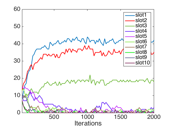
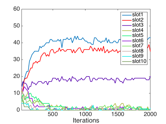
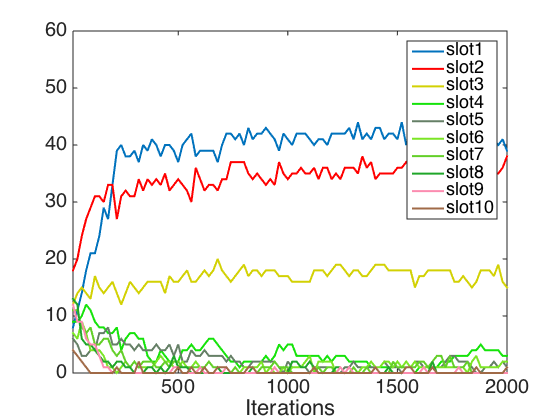
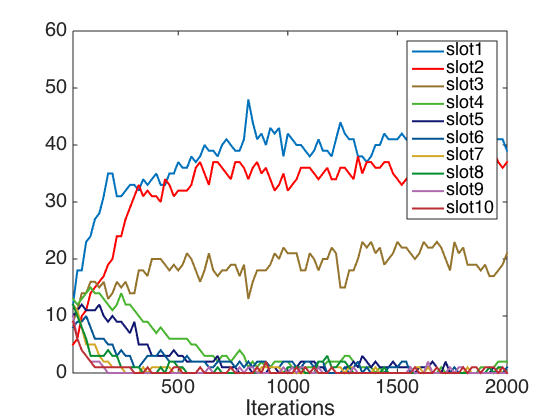
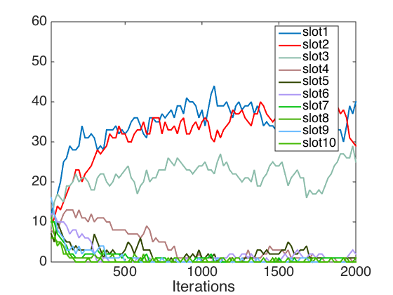
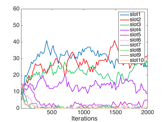
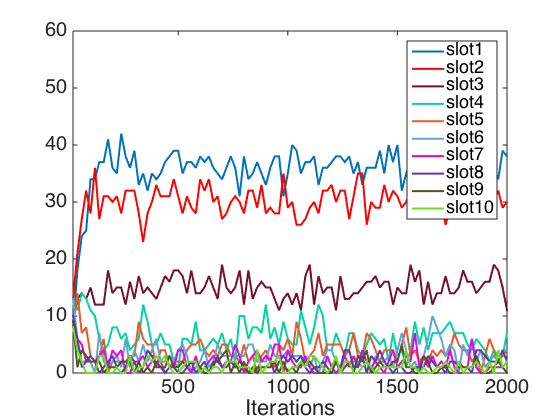
Simulation results with diminishing exploration rates. As discussed in Section 4.4, we restrict the exploration rates to be $\mathbf{p}$-series. In particular, Figures 2 - 4 show the evaluations of the RL algorithm for three cases $\epsilon_{i}(t)=\frac{1}{10}t^{-\frac{0.25}{100}}$, $\epsilon_{i}(t)=\frac{1}{10}t^{-\frac{0.5}{100}}$ and $\epsilon_{i}(t)=\frac{1}{10}t^{-\frac{1}{100}}$ (the optimal one), respectively. The exploration deviations are chosen as $e_{i}(t)=\frac{9}{10t^{2}}$ and the measurement noises are absent; i.e., $w_{i}(t)=0$. The duration of the simulation is 2,000 iterations. The simulation results confirm the convergence of the action profiles in Theorem 1. In addition, the convergence in Figure 4 is fastest where the optimal exploration rates $\epsilon_{i}(t)=\frac{1}{10}t^{-\frac{1}{100}}$ are adopted. It is consistent with the discussion in Section 4.4.

Simulation results with measurement errors. In this part, we evaluate how the RL algorithm performs when the measurement noises are present. The exploration rates are chosen as $\epsilon_{i}(t)=\frac{1}{10}t^{-\frac{1}{100}}$ and the exploration deviations are chosen as $e_{i}(t)=\frac{9}{10t^{2}}$. The measurement noises are chosen as uniformly distributed over two different intervals $[-10,10]$ and $[-20,20]$, respectively. Compared with Figure 4, Figures 5 - 6 show that the action profiles slow down and oscillate with larger magnitudes when the noise magnitude increases. In addition, we also evaluate how the RL algorithm performs when Assumption 1 is violated. In particular, $w_{i}(t)$ is uniformly distributed over the time-dependent interval $[-10\log(t),10\log(t)]$. The result shown in Figures 7 implies that the action profiles do not converge anymore.

Figure 5: Temporal aggregate demands allocated at ten time slots with uniformly distributed measurement noises in the interval $[-10,10]$.

Figure 6: Temporal aggregate demands allocated at ten time slots with uniformly distributed measurement noises in the interval $[-20,20]$.

Figure 7: Temporal aggregate demands allocated at ten time slots with uniformly distributed measurement noises in the interval $[-10\ln(t),10\ln(t)]$.

Matlab simulation results with fixed exploration rates. Figures 8 shows the evaluation of the RL algorithm with fixed exploration rates $\epsilon_{i}(t)=\frac{1}{10}^{-\frac{1}{100}}$. The exploration deviations are chosen as $e_{i}(t)=\frac{9}{10t^{2}}$ and the measurement noises are absent; i.e., $w_{i}(t)=0$. The comparison of Figures 4 and 8 shows that fixed exploration rates cause larger oscillations in steady state.

Figure 8: Temporal aggregate demands allocated at ten time slots with fixed exploration rates $\epsilon_{i}(t)=\frac{1}{10}^{-\frac{1}{100}}$.

6.2 Case 2: Adaptive cyber defense scenario

Table 1: Utility table

Defense actions	Attack actions
	(0,10)	(1,9)	(2,8)	(3,7)	(4,6)	(5,5)	(6,4)	(7,3)	(8,2)	(9,1)	(10,0)
$d_{1}$(Fedora 11)	0,1.0	0.1,0.9	0.2,0.8	0.3,0.7	0.4,0.6	0.5,0.5	0.6,0.4	0.7,0.3	0.8,0.2	0.9,0.1	1.0,0
$d_{2}$(Gentoo 9)	1.0,0	0.9,0.1	0.8,0.2	0.7,0.3	0.6,0.4	0.5,0.5	0.4,0.6	0.3,0.7	0.2,0.8	0.1,0.9	0,1.0
$d_{3}$(CentOS 6.3)	0,1.0	0.1,0.9	0.2,0.8	0.3,0.7	0.4,0.6	0.5,0.5	0.6,0.4	0.7,0.3	0.8,0.2	0.9,0.1	1.0,0
$d_{4}$(Debian 6)	1.0,0	1.0,0	1.0,0	1.0,0	1.0,0	1.0,0	1.0,0	1.0,0	1.0,0	1.0,0	1.0,0
$d_{5}$(FreeBSD 9)	1.0,0	1.0,0	1.0,0	1.0,0	1.0,0	1.0,0	1.0,0	1.0,0	1.0,0	1.0,0	1.0,0

In this section, we study a real-world cyber security scenario which consists of two players: the defender and attacker. The system is the server containing several zero-day security vulnerabilities. A zero-day attack happens once that a software/hardware vulnerability is exploited by the attacker before software the engineers develop any patch to fix the vulnerability. The attacker is equipped with a set of zero-day attack scripts denoted as $\mathcal{A}$ and the defender is equipped with a set of platforms denoted as $\mathcal{D}$. The defender uses a defensive technique called dynamic platforms Okhravi et al. (2014), which changes the properties of the server such that it is harder for the attacker to succeed. The components in the cyber security scenario and the interactions among the components will be discussed in the following paragraphs.

6.2.1 System components

Defender. The defender has a set of different platforms; e.g., different versions of operating systems and architectures. The defender periodically restarts the server, chooses one platform from $\mathcal{D}$ and deploys it on the server each time it restarts the server. The iteration denoted in Section 2.1 is the defense period in this scenario. The action $d(t)$ is the platform deployed at iteration $t$.

Attacker. The attacker has a set of zero-day attack scripts, where each attack script can only succeed on some platforms, but no the others. The attacker periodically chooses one of the attack scripts to attack the server. Notice that the attack period is often smaller than the defense period because the defender cannot restart the server too frequently due to the resource consumption of restarting the server. In fact, the defense period is usually a multiple of the attack period. The attack action at iteration $t$, denoted as $a(t)$, is a subset of the attack scripts and the attack action set $\mathcal{A}$ includes all possible subsets. The order of choosing the attack scripts in one iteration does not matter.

Server. Once an attack action succeeds, the attacker can control the server for a certain amount of time. And every time the server restarts, the defender takes over the control of the server. And here we assume the time consumed by the attack scripts to succeed and the time consumed by restarting the server are negligible compared with the length of an iteration.

Utility. The goal of both the attacker and defender is to gain longer control time of the server. The utility of the defender $u_{d}(d(t),a(t))$ is the fraction of the time controlled by the defender during iteration $t$ and the utility of the attacker $u_{a}(d(t),a(t))$ is the fraction of the time controlled by the attacker. Notice that $u_{d}(d(t),a(t))+u_{a}(d(t),a(t))=1$.

Informational constraint. The attacker can observe when the server restarts, so it knows the iterations, but it does not know the defender’s action set $\mathcal{D}$ and which platform is deployed. The defender does not know the attacker’s action set $\mathcal{A}$ and the specific attack scripts chosen by the attacker. At the end of each defense period, both the defender and attacker can measure how much time they control the server. Therefore, each player only knows its own utility values instead of the structure of the utility function.

6.2.2 Evaluation

Evaluation setup. In this section, we use Matlab simulations to evaluate the performance of our algorithm based on real-world platform settings, attack scripts and server control data (Okhravi et al., 2012, 2014). The total number of defense actions is 5; i.e., the defender has five different platforms: Fedora 11 on x86, Gentoo 9 on x86, Debian 6 on x86, FreeBSD 9 on x86, and CentOS 6.3 on x86. The attacker has two zero-day attack scripts: TCP MAXSEG exploit, and Socket Pairs exploit. The defense period is set to be ten times as large as the attack period; i.e., during one iteration, the attacker launches 10 attack scripts. Since the time consumed by the attack scripts to succeed is negligible, one attack script enables the attacker control $\frac{1}{10}$ of the iteration if it succeeds. The total number of attack actions is 11; i.e., $a_{1}=(0,10),a_{2}=(1,9),\cdots,a_{11}=(10,0)$, where $a(t)=(0,10)$ means the attacker launches 0 TCP MAXSEG exploit and 10 Socket Pairs exploits at iteration $t$.

Real-world utility values. Based on the evaluation setup and the real-world attack scripts, we first replay different attack actions on different platforms to get the utility table for the defender and the attacker. The results are shown in Table 1, where the defender is the row player and the attacker is the column player. In each cell, the first number represents the utility value to the defender, and the second number represents the utility value to the attacker.

Nash equilibrium. By Proposition 1 in Takahashi and Yamamori (2002), we know any 2-player finite game and its any sub-game (any game constructed by restricting the set of actions to a subset of the set of actions in the original game) has at least one pure Nash equilibrium is a weakly acyclic game. From Table 1, we can see any sub-game has at least one pure Nash equilibrium. Now we want to calculate the pure Nash equilibrium (equilibria). From Table 1, we can see if the defense strategy is $d_{4}$ (deploying Debian 6) or $d_{5}$ (deploying FreeBSD 9), then the utility of the defender is 1 (the utility of the attacker is 0) not matter what action the attacker uses. From Definition 1 and Remark 2, we know the combinations of any attacker action and defense action $d_{4}$ or $d_{5}$ are pure Nash equilibria.

Figure 9: Trajectories of attack $a(t)$ and defense $d(t)$ with diminishing exploration rate $\epsilon_{d}(t)=\epsilon_{a}(t)=\frac{1}{11t^{1/2}}$.

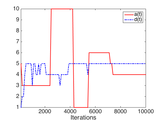
Simulation results with optimal exploration rates. Based on Table 1, we simulate the interactions of the defender and attacker in Matlab. We choose the exploration rates $\epsilon_{d}(t)=\epsilon_{a}(t)=\frac{1}{11t^{1/2}}$., the optimal one among $\mathbf{p}$-series as discussed in Section 4.4. The exploration deviations are chosen as $e_{d}(t)=\frac{1}{110t^{2}}$ and $e_{a}(t)=\frac{1}{110t^{2}}$. We assume that the measurement noises are absent; i.e., $w_{d}(t)=w_{a}(t)=0$. The duration of each simulation (from the attack begins till the attack ends) is 10,000 iterations and we repeat 100 identical simulations. Figure 9 shows the trajectories of the defense and attack actions in one certain simulation. And for each simulation, we record the defense action at each iteration. Then at each iteration $t$, we have 100 chosen defense actions and we use the number of each defense action over 100 as the probability of choosing such defense action at $t$. The result in Figure 9 suggests that the defense action converges to the set $\{d_{4},d_{5}\}$. Notice that the combinations of any attacker action and defense action $d_{4}$ or $d_{5}$ are pure Nash equilibria. Then the simulation results confirm that the convergence of the action profiles to the set of pure Nash equilibria.

7 Conclusion

This paper investigates a class of multi-player discrete games where each player aims to maximize its own utility function with limited information about the game of interest. We propose the RL algorithm which converges to the set of action profiles which have maximal stochastic potential with probability one. The convergence rate of the proposed algorithm is analytically quantified. Moreover, the performance of the algorithm is verified by two case studies in the smart grid and cybersecurity.

References

- Abramowitz and Stegun (1964) Abramowitz, M., Stegun, I. A., 1964. Handbook of mathematical functions: with formulas, graphs, and mathematical tables. Vol. 55. Courier Corporation.
- Altman et al. (2002) Altman, E., Basar, T., Srikant, R., Jun 2002. Nash equilibria for combined flow control and routing in networks: Asymptotic behavior for a large number of users. IEEE Transactions on Automatic Control 47 (6), 917–930.
- Arrow and Debreu (1954) Arrow, K., Debreu, G., 1954. Existence of an equilibrium for a competitive economy. Econometrica 22, 265–290.
- Arslan et al. (2007) Arslan, G., Marden, J. R., Shamma, J. S., 2007. Autonomous vehicle-target assignment: A game-theoretical formulation. ASME Journal on Dynamic Systems, Measurement, and Control 129 (5), 584–596.
- Basar and Olsder (1999) Basar, T., Olsder, G., 1999. Dynamic noncooperative game theory. SIAM Classics in Applied Mathematics.
- Bertsekas (2015) Bertsekas, D. P., 2015. Convex Optimization Algorithms. Athena Scientific.
- Cayley (1889) Cayley, A., 1889. A theorem on trees. Quartery Journal of Mathematics 23, 376–378.
- Chlebus (2009) Chlebus, E., 2009. An approximate formula for a partial sum of the divergent p-series. Applied Mathematics Letters 22 (5), 732 – 737.
- Facchinei and Kanzow (2007) Facchinei, F., Kanzow, C., 2007. Generalized Nash equilibrium problems. 4OR 5 (3), 173–210.
- Foster and Young (1990) Foster, D., Young, P., 1990. Stochastic evolutionary game dynamics∗. Theoretical Population Biology 38 (2), 219 – 232.
- Freidlin et al. (2012) Freidlin, M. I., Szücs, J., Wentzell, A. D., 2012. Random perturbations of dynamical systems. Vol. 260. Springer Science & Business Media.
- Frihauf et al. (2012) Frihauf, P., Krstic, M., Basar, T., 2012. Nash equilibrium seeking in non-cooperative games. IEEE Transcations on Automatic Control 57 (5), 1192–1207.
- Fudenberg and Levine (1998) Fudenberg, D., Levine, D. K., 1998. The theory of learning in games. Vol. 2. MIT Press.
- Hasʹminskii and Silver (1972) Hasʹminskii, R. Z., Silver, B., 1972. Stochastic approximation and recursive estimation. Vol. 47. American Mathematical Soc.
- Hatanaka et al. (2016) Hatanaka, T., Wasa, Y., Funada, R., Charalambides, A. G., Fujita, M., 2016. A payoff-based learning approach to cooperative environmental monitoring for ptz visual sensor networks. IEEE Transactions on Automatic Control 61 (3), 709–724.
- Huang and Manton (2009) Huang, M., Manton, J. H., 2009. Coordination and consensus of networked agents with noisy measurements: Stochastic algorithms and asymptotic behavior. SIAM Journal on Control and Optimization 48 (1), 134–161.
- Koshal et al. (2013) Koshal, J., Nedić, A., Shanbhag, U. V., March 2013. Regularized iterative stochastic approximation methods for stochastic variational inequality problems. IEEE Transactions on Automatic Control 58 (3), 594–609.
- Kushner and Yin (2003) Kushner, H., Yin, G., 2003. Stochastic Approximation and Recursive Algorithms and Applications. Springer.
- Liu and Krstic (2011) Liu, S., Krstic, M., 2011. Stochastic Nash equilibrium seeking for games with general nonlinear payoffs. SIAM Journal on Control and Optimization 49 (4), 1659–1679.
- Marden et al. (2013) Marden, J. R., Ruben, S. D., Pao, L. Y., July 2013. A model-free approach to wind farm control using game theoretic methods. IEEE Transactions on Control Systems Technology 21 (4), 1207–1214.
- Marden et al. (2009) Marden, J. R., Young, H. P., Arslan, G., Shamma, J. S., 2009. Payoff-based dynamics for multiplayer weakly acyclic games. SIAM Journal on Control and Optimization 48 (1), 373–396.
- Monderer and Shapley (1996) Monderer, D., Shapley, L., 1996. Potential games. Games and Economic Behavior 14 (1), 124 – 143.
- Nisan et al. (2007) Nisan, N., Roughgarden, T., Tardos, E., Vazirani, V. V., 2007. Algorithmic game theory. Vol. 1. Cambridge University Press Cambridge.
- Okhravi et al. (2012) Okhravi, H., Comella, A., Robinson, E., Haines, J., 2012. Creating a cyber moving target for critical infrastructure applications using platform diversity. International Journal of Critical Infrastructure Protection 5 (1), 30–39.
- Okhravi et al. (2014) Okhravi, H., Riordan, J., Carter, K., Sep 2014. Quantitative evaluation of dynamic platform techniques as a defensive mechanism. In: Research in Attacks, Intrusions and Defenses: 17th International Symposium, RAID 2014. Gothenburg, Sweden, pp. 405–425.
- Palomar and Eldar (2010) Palomar, D., Eldar, Y., 2010. Convex optimization in signal processing and communications. Cambridge University Press.
- Pang et al. (2008) Pang, J.-S., Scutari, G., Facchinei, F., Wang, C., 2008. Distributed power allocation with rate constraints in Gaussian parallel interference channels. IEEE Transactions on Information Theory 54 (8), 3471–3489.
- Rosen (1965) Rosen, J., 1965. Existence and uniqueness of equilibrium points for concave N-person games. Econometrica 33 (3), 520–534.
- Roumboutsos and Kapros (2008) Roumboutsos, A., Kapros, S., 2008. A game theory approach to urban public transport integration policy. Transport Policy 15 (4), 209 – 215.
- Sandholm (2010) Sandholm, W. H., 2010. Population games and evolutionary dynamics. MIT Press.
- Stankovic et al. (2012) Stankovic, M., Johansson, K., Stipanovic, D., 2012. Distributed seeking of Nash equilibria with applications to mobile sensor networks. IEEE Transcations on Automatic Control 57 (4), 904–919.
- Takahashi and Yamamori (2002) Takahashi, S., Yamamori, T., 2002. The pure Nash equilibrium property and the quasi-acyclic condition. Economics bulletin 3 (22), 1–6.
- Uspensky (1937) Uspensky, J. V., 1937. Introduction to mathematical probability. New York ; London : McGraw-Hill.
- Wang et al. (2012) Wang, G., Shanbhag, U. V., Meyn, S. P., Dec 2012. On Nash equilibria in duopolistic power markets subject to make-whole uplift. In: 2012 IEEE 51st IEEE Conference on Decision and Control (CDC). Maui, Hawaii, USA, pp. 472–477.
- Xiao et al. (2007) Xiao, L., Boyd, S., Kim, S.-J., 2007. Distributed average consensus with least-mean-square deviation. Journal of Parallel and Distributed Computing 67 (1), 33 – 46.
- Yin et al. (2011) Yin, H., Shanbhag, U., Mehta, P., 2011. Nash equilibrium problems with scaled congestion costs and shared constraints. IEEE Transactions on Automatic Control 56 (7), 1702–1708.
- Young (1993) Young, H. P., 1993. The evolution of conventions. Econometrica: Journal of the Econometric Society 61, 57–84.
- Young (2001) Young, H. P., 2001. Individual strategy and social structure: An evolutionary theory of institutions. Princeton University Press.
- Yousefian et al. (2013) Yousefian, F., Nedić, A., Shanbhag, U. V., June 2013. A distributed adaptive steplength stochastic approximation method for monotone stochastic Nash games. In: 2013 American Control Conference. pp. 4765–4770.
- Zhu (2014) Zhu, M., Jul 2014. Distributed demand response algorithms against semi-honest adversaries. In: IEEE Power and Energy Society General Meeting. No. 943. National Harbor, MD.
- Zhu and Frazzoli (2016) Zhu, M., Frazzoli, E., 2016. Distributed robust adaptive equilibrium computation for generalized convex games. Automatica 63 (1), 82–91.
- Zhu et al. (2014) Zhu, M., Hu, Z., Liu, P., Nov 2014. Reinforcement learning algorithms for adaptive cyber defense against Heartbleed. In: First ACM Workshop on Moving Target Defense in Association with 2014 ACM Conference on Computer and Communications Security(MTD ’14). Scottsdale, Arizona, USA, pp. 51–58.
- Zhu and Martínez (2013) Zhu, M., Martínez, S., 2013. Distributed coverage games for energy-aware mobile sensor networks. SIAM Journal on Control and Optimization 51 (1), 1–27.