Application of Mössbauer effect to study subnanometer harmonic displacements in a thin solid

Abstract

We measure subnanometer displacements of thin samples vibrated by piezotransducer. Samples contain ⁵⁷Fe nuclei, which are exposed to 14.4 keV $\gamma$-radiation. Vibration produces sidebands from a single absorption line of the sample. The sideband intensities depend on the vibration amplitude and its distribution along the sample. We developed a model of this distribution, which adequately describes the spectra of powder and stainless steel (SS) absorbers. We propose to filter $\gamma$-radiation through a small hole in the mask, placed before the absorber. In this case only a small spot of the vibrated absorber is observed. We found for SS foil that nuclei, exposed to $\gamma$-radiation in this small spot, vibrate with almost the same amplitudes whose difference does not exceed a few picometers.

I Introduction

A scanning tunneling microscope (STM) demonstrates remarkable lateral and depth resolution. STM proved to be an excellent instrument for imaging surfaces at the atomic level. Its development earned its inventors, Binning and Rohrer, the Nobel prize in Physics in 1986. Information is acquired by monitoring the tunneling current as a function of tip position, applied voltage, and local density of states. If local density of states is not well known, then STM needs calibration. To solve the problem of absolute calibration of the conducting tip displacement an etalon step is usually grown on the surface of the sample. Recently, fluorescence microscopy with nanoscale spatial resolution was invented, see the review by Stefan Hell Ref. Hell , the Nobel prize winner in Chemistry in 2014. This method allows to overcome diffraction limit. Meanwhile, if we could apply $\gamma$-radiation for spatial measurements, then Angstrom resolution scale could be achieved.

In this paper we discuss the application of $\gamma$-photons for sub-nanometer spatial measurements with sub-Angstrom resolution. We employ 14.4 keV $\gamma$-photons, emitted by radioactive ⁵⁷Co with a wavelength 86 pm. Since we are not able to focus $\gamma$-radiation field and direct it to a desirable spot on the sample, we address to the spectral measurements. In our case, not a fluorescence, but transmission spectra of the sample, containing resonant nuclei ⁵⁷Fe, are proposed to be measured. We expect high depth resolution, while lateral resolution could be controlled by a mask with a small hole, which is moved along the surface of the sample. We expect that our method could provide controllable and calibrated displacements of the surface with sub-Angstrom resolution for calibrating, for example, STM.

In our method the sample containing resonant nuclei is mechanically vibrated. As a result, along with the main absorption line, a system of satellites appears in the spectrum, spaced apart at distances that are multiples of the vibration frequency. Line intensities of this comb structure are very sensitive to the vibration amplitude, which is extremely small (Angstrom or even smaller). For the stainless steel foil, which is illuminated by $\gamma$-radiation transmitted through a small hole in the mask placed before the absorber, we measured displacements of the order of dozens of picometers with the accuracy of a few picometers.

The influence of extremely-small-amplitude mechanical vibrations of the absorbers containing Mössbauer nuclei attracted attention since the invention of Mössbauer spectroscopy. Mössbauer sidebands, produced from a single parent line by absorber vibration, were observed in many different samples Ruby ; Cranshaw ; Mishroy ; Kornfeld ; Walker ; Mkrtchyan77 ; Perlow ; Monahan ; Mkrtchyan79 ; Shvydko89 ; Shvydko92 . However, the intensity of the sidebands has not been yet satisfactory explained Walker ; Mkrtchyan77 ; Mkrtchyan79 . There are two models of coherent and incoherent vibrations of nuclei in the absorber Cranshaw ; Walker ; Mishroy ; Kornfeld ; Mkrtchyan77 ; Mkrtchyan79 . Coherent model implies piston-like vibration of the absorber with frequency $\Omega$ and phase $\psi$ along the propagation direction of $\gamma$ quanta. This model predicts the intensity of the $n$-th sideband proportional to the square of Bessel function $J_{n}^{2}(m)$, where $m=2\pi a_{0}/\lambda$ is the modulation index, which is proportional to the ratio of the amplitude of the harmonic displacements $a_{z}(t)=a_{0}\sin(\Omega t+\psi)$ and the wavelenght $\lambda$ of $\gamma$-photon. Incoherent model, proposed by Abraham Abragam , is based on the Rayleigh distribution of the nuclear-vibration amplitudes in the absorber predicting the intensity proportional to $\exp(-m^{2})I_{n}(m^{2})$, where $I_{n}(m^{2})$ is the modified Bessel function. However, both models or their combinations cannot describe perfectly all absorption spectra, which are experimentally observed for samples of different mechanical properties and chemical composition. To support this statement we refer to Chien and Walker who pointed out in Ref. Walker that while unequivocally measured intensities agree qualitatively with Abragam’s sideband theory, no existing theory at present can account quantitatively for the sideband intensities since the amplitude distribution that satisfactorily describes the data are not known at present.

We propose a heuristic distribution of nuclear-vibration amplitudes, which is derived from the Gaussian distribution with appropriate modifications. Our model provides good fitting of experimental spectra. Depending on a parameter of the model $\sigma$, the proposed distribution tends to a delta-like, inherent to the coherent model if $\sigma\rightarrow 0$, or it tends to the Rayleigh distribution inherent to the incoherent model if $\sigma\rightarrow 0.72$.

The proposed model allows to determine from experimental data the amplitude of subnanometer harmonic displacements of the absorber with an accuracy less than half Angstrom. Our method consists of two steps. First, we apply our heuristic distribution to fit experimental spectra to the model. This fitting gives the parameter $\sigma$, which specifies the appropriate distribution of the displacements irrespective to their location in the sample. Second, we construct an actual distribution of the vibration amplitudes across the surface of the absorber, which is consistent with our heuristic distribution.

Two absorbers are experimentally studied, i.e., K₄Fe(CN)${}_{6}\cdot 3$H₂O powder enriched by ⁵⁷Fe and stainless steel (SS) foil with natural abundance of ⁵⁷Fe. For powder, the distribution of the powder-grain displacements, obtained from the spectrum fitting, is close to the continuous uniform distribution with wide scattering of the vibration amplitudes, which is very different from the Rayleigh distribution. For SS foil we found that the displacement distribution along the surface of a thin foil is close to the narrow bell-shape distribution. Physical interpretation of these results is discussed.

For SS foil we experimentally verified our conclusions placing a mask just in the front of the absorber. We made a hole in the mask and compared the observed Mössbauer spectra with our theoretical predictions. We observed a change of Mössbauer spectra with decrease of the size of the hole, which firmly supports our model. We moved the narrowest hole of the mask along the surface of the vibrated SS foil and could detect the change of the vibration amplitude along the SS foil, which is deduced from the spectrum analysis. In addition to a scientific value of our model giving an explanation of properties of the Mössbauer sidebands produced by the absorber vibration, we expect that our findings could give an impetus to the development of the method measuring extra-small displacements with an accuracy less than half Angstrom.

II Coherent and incoherent models of the mechanical vibrations of the absorber

The propagation of $\gamma$ radiation through a resonant Mössbauer medium vibrating with frequency $\Omega$ may be treated classically Lynch . In this approach the radiation field from the source nucleus after passing through a small diaphragm is approximated as a plane wave propagating along the direction $\mathbf{z}$. In the coordinate system rigidly bounded to the absorbing sample, the field, seen by the absorber nuclei, is described by

$$E_{S}(t-t_{0})\propto\theta(t-t_{0})e^{-(i\omega_{S}+\Gamma_{0}/2)(t-t_{0})+ikz+i\varphi(t)},$$ (1)

where $\omega_{S}$ and $k$ are the carrier frequency and the wave number of the radiation field, $1/\Gamma_{0}$ is the lifetime of the excited state of the emitting source nucleus, $t_{0}$ is the instant of time when the excited state is formed, $\Theta(t-t_{0})$ is the Heaviside step-function, $\varphi(t)=2\pi a_{z}(t)/\lambda=m\sin(\Omega t+\psi)$ is a time dependent phase of the field due to a piston-like periodical displacement $a_{z}(t)$ of the absorber with respect to the source, $\psi$ is a vibration phase, and $\lambda$ is the radiation wavelength.

The radiation field (1) can be expressed as polychromatic radiation with a set of spectral lines $\omega_{S}-n\Omega$ ($n=0$, $\pm 1$, $\pm 2$, …), i.e.,

$$E_{S}(t-t_{0})=E_{C}(t-t_{0})e^{-i\omega_{S}(t-t_{0})+ikz}\sum_{n=-\infty}^{+\infty}J_{n}(m)e^{in(\Omega t+\psi)},$$ (2)

where $E_{C}(t-t_{0})=E_{0}\theta(t-t_{0})e^{-\Gamma_{0}(t-t_{0})/2}$ is the common part of the field components, $E_{0}$ is the field amplitude, and $J_{n}(a)$ is the Bessel function of the $n$th order. The Fourier transform of this field has a frequency comb structure

$$E_{S}(\omega)=E_{0}\sum_{n=-\infty}^{+\infty}\frac{J_{n}(a)e^{in(\Omega t_{0}+\psi)}}{\Gamma_{0}/2+i(\omega_{S}-n\Omega-\omega)},$$ (3)

where for shortening of notations the exponential factor with $ikz$ is omitted. From this expression, it follows that the vibrating absorber ‘sees’ the incident radiation as an equidistant frequency comb with spectral components $\omega_{S}-n\Omega$ whose amplitudes are proportional to the Bessel function $J_{n}(m)$.

The Fourier transform of the radiation field is changed at the exit of the resonant absorber as (see Lynch ; Monahan ; Vagizov ; Shakhmuratov15 )

$$E_{\text{out}}(\omega)=E_{0}\sum_{n=-\infty}^{+\infty}\frac{J_{n}(m)\exp\left[in(\Omega t_{0}+\psi)-\frac{b}{\Gamma_{A}/2+i(\omega_{A}-\omega)}\right]}{\Gamma_{0}/2+i(\omega_{S}-n\Omega-\omega)},$$ (4)

where $\omega_{A}$ and $\Gamma_{A}$ are the frequency and linewidth of the absorber, $b=T_{A}\Gamma_{0}/4$ is the parameter depending on the effective thickness of the absorber $T_{A}=fn_{A}\sigma_{A}$, $f$ is the Debye-Waller factor, $n_{A}$ is the number of ⁵⁷Fe nuclei per unit area of the absorber, and $\sigma_{A}$ is the resonance absorption cross section. The source linewidth $\Gamma_{S}$ can be different from $\Gamma_{0}$ due to the contribution of the environment of the emitting nucleus in the source. In this case $\Gamma_{0}$ can be simply substituted by $\Gamma_{S}$ in Eq. (4). Here, nonresonant absorption is disregarded. Recoil processes in nuclear absorption and emission are not taken into account assuming that recoilless fraction (Debye-Waller factor) is $f=1$. These processes can be easily taken into account in experimental data analysis.

Time dependence of the amplitude of the output radiation field is found by inverse Fourier transformation

$$E_{\text{out}}(t-t_{0})=\frac{1}{2\pi}\int_{-\infty}^{+\infty}E_{\text{out}}(\omega)e^{-i\omega(t-t_{0})}d\omega.$$ (5)

In the laboratory reference frame this field is transformed as

$$E_{\text{lab}}(t-t_{0})=E_{\text{out}}(t-t_{0})e^{-i\varphi(t)}.$$ (6)

Since the fields $E_{\text{lab}}(t-t_{0})$ and $E_{\text{out}}(t-t_{0})$ differ only in the phase $\varphi(t)$, the intensity seen by the detector, $I_{\text{lab}}(t-t_{0})=\left|E_{\text{lab}}(t-t_{0})\right|^{2}$, coincides with the intensity of the radiation field in the vibrated reference frame $I_{\text{lab}}(t-t_{0})=\left|E_{\text{lab}}(t-t_{0})\right|^{2}$, i.e.,

$$I_{\text{lab}}(t-t_{0})=I_{\text{out}}(t-t_{0}).$$ (7)

This condition is valid if we use the detection scheme, which is not sensitive to the spectral content of the radiation field filtered by the vibrated absorber. If the second absorber (spectrum analyzer) is placed between the vibrated source and detector, then another description of the radiation intensity is necessary Shvydko89 ; Shvydko92 .

Since we don’t use a second single line resonance filter analyzing the spectra of $\gamma$ radiation emerging from the vibrated absorber, the intensity of the field, registered by a detector, can be described by expression

$$I_{\text{out}}(t-t_{0})=\frac{1}{(2\pi)^{2}}\int_{-\infty}^{+\infty}d\omega_{1}\int_{-\infty}^{+\infty}d\omega_{2}E_{\text{out}}(\omega_{1})E_{\text{out}}^{\ast}(\omega_{2})e^{i(\omega_{2}-\omega_{1})(t-t_{0})}.$$ (8)

Thus, in our case the radiation intensity at the exit of the vibrating absorber is the same if the source is vibrated instead of absorber.

Frequency-domain Mössbauer spectrum is measured by counting the number of photons, detected within long time windows of the same duration for all resonant detunings, which are varied by changing the value of a velocity of the Mössbauer drive moving the source. Time windows are not synchronized with the mechanical vibration and their duration $T_{\text{w}}$ is much longer than the oscillation period $T_{\text{osc}}=2\pi/\Omega$. Since the emission time of $\gamma$-photons is random, the observed radiation intensity is averaged over $t_{0}$

$$\left\langle I_{\text{out}}(t-t_{0})\right\rangle_{t_{0}}\propto\frac{1}{T_{w}}\int_{-T_{\text{w}}/2}^{+T_{\text{w}}/2}I_{\text{out}}(t-t_{0})dt_{0},$$ (9)

where for simplicity we assume that $T_{\text{w}}\rightarrow\infty$. Then the observed number of photon counts, which is proportional to the intensity, i.e., $N_{\text{out}}(\Delta)=\left\langle I_{\text{out}}(t-t_{0})\right\rangle_{t_{0}}$, varies with the change of the resonant detuning $\Delta=\omega_{A}-\omega_{S}$ as

$$N_{\text{out}}(\Delta)=\sum_{n=-\infty}^{+\infty}J_{n}^{2}(m)B_{n}(\Delta),$$ (10)

where

$$B_{n}(\Delta)=\frac{\Gamma_{S}}{2\pi}\int_{-\infty}^{+\infty}\frac{e^{-\frac{b\Gamma_{A}}{(\Gamma_{A}/2)^{2}+(\Delta+n\Omega-\omega)^{2}}}}{(\Gamma_{S}/2)^{2}+\omega^{2}}d\omega.$$ (11)

II.1 Coherent model

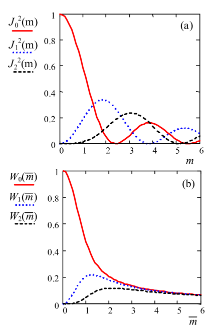
Figure 1: (color on line) (a) The dependence of the intensities of the central component (solid line in red), first satellite (dotted line in blue), and second satellite (dashed line in black) on the modulation index $m$ for the coherent model. (b) The dependence of the averaged intensities of the central component (solid line in red), first satellite (dotted line in blue), and second satellite (dashed line in black) on $\bar{m}$, which is the square root of the modulation index deviation $\langle m^{2}\rangle$ in the incoherent model.

If all the nuclei in the absorber vibrate with the same phase and amplitude, then a single parent line is transformed into a set of spectral lines $\omega_{S}\pm n\Omega$ ($n=0,1,2,...$) spaced apart at distances that are multiples of the oscillation frequency. The intensity of the $n$th sideband is given by the square of the Bessel function $J_{n}^{2}(m)$. According to this theoretical prediction the line intensities oscillate with increase of the modulation index $m$, see Fig. 1(a). For example, the first sidebands, whose intensities are proportional to $J_{\pm 1}^{2}(m)$ take their global maxima when $m=1.8$, while the intensity of the central component $J_{0}^{2}(m)$ is zero if $m=2.4$. A model of uniform and phased vibrations of all the nuclei in the absorber is named the coherent model. Unfortunately, experiments with powder absorbers did not demonstrate oscillatory dependence of the sideband intensities on the modulation index. Even in many experiments the intensity of the central component was always the strongest, while the intensity of the satellites, initially increasing with the modulation amplitude increase, then monotonically decreased as a function of $m$. Meanwhile, experiments with stainless foil Mkrtchyan77 ; Mkrtchyan79 showed appreciable decrease of the central component of the spectrum to the level of the sidebands with increase of the modulation index $m$ and some oscillating dependencies of the spectral components on $m$.

II.2 Incoherent model

The incoherent model was proposed Ruby ; Cranshaw ; Mishroy ; Kornfeld ; Walker to explain the discrepancy between the coherent model and the experiment. It is based on the Abragam model Abragam suggesting that the motion of nuclei in the absorber can be described as the sum of two vibrations along the propagation direction $\mathbf{z}$ of $\gamma$ photon, i.e., $\mathbf{a}_{z}(t)=a_{x}\cos(\Omega t+\psi)+a_{y}\sin(\Omega t+\psi)$, where $a_{x}$ and $a_{y}$ are the amplitudes, which are different for different coordinates $x$ and $y$ in the plane of the absorber surface and in this sense $\mathbf{a}_{z}(t)$ is a vector Cranshaw . These amplitudes are Gaussian-distributed, centered at zero, and independent. Then, their distribution is described by the function

$$G(a_{x,y},\left\langle a_{x,y}^{2}\right\rangle)=\frac{\exp\left(-\frac{a_{x,y}^{2}}{2\left\langle a_{x,y}^{2}\right\rangle}\right)}{\sqrt{2\pi\left\langle a_{x,y}^{2}\right\rangle}},$$ (12)

where $\left\langle a_{x,y}^{2}\right\rangle$ is variance, which is not zero, while $\left\langle a_{x,y}\right\rangle=0$. The amplitude of the vector $\mathbf{a}_{z}(t)$ is $a_{z}=\sqrt{a_{x}^{2}+a_{y}^{2}}$. If $\left\langle a_{x}^{2}\right\rangle=\left\langle a_{y}^{2}\right\rangle=\overline{a^{2}}$, the amplitude $a_{z}$ is distributed as

$$P_{R}(a_{z},\overline{a^{2}})=\int_{-\infty}^{+\infty}da_{x}\int_{-\infty}^{+\infty}da_{y}\frac{\exp\left(-\frac{a_{x}^{2}+a_{y}^{2}}{2\overline{a^{2}}}\right)}{2\pi\overline{a^{2}}}\delta(a_{z}-\sqrt{a_{x}^{2}+a_{y}^{2}}).$$ (13)

In a polar coordinate system $(r,\phi)$ this distribution is transformed to

$$P_{R}(a_{z},\overline{a^{2}})=\int_{0}^{2\pi}d\phi\int_{-\infty}^{+\infty}dr\frac{\exp\left(-\frac{r^{2}}{2\overline{a^{2}}}\right)}{2\pi\overline{a^{2}}}\delta(r-a_{z}),$$ (14)

which gives the Rayleigh distribution

$$P_{R}(a_{z},\overline{a^{2}})=\frac{a_{z}}{\overline{a^{2}}}\exp\left(-\frac{a_{z}^{2}}{2\overline{a^{2}}}\right).$$ (15)

Averaging the intensity of the $n$th sideband with this distribution

$$W_{n}(\overline{m})=\int_{0}^{\infty}P_{R}(a_{z},\overline{a^{2}})J_{n}\left(\frac{2\pi a_{z}}{\lambda}\right)da_{z},$$ (16)

one obtains

$$W_{n}(\overline{m})=e^{-\left\langle m^{2}\right\rangle}I_{n}\left(\left\langle m^{2}\right\rangle\right),$$ (17)

where $\left\langle m^{2}\right\rangle=(2\pi/\lambda)^{2}\overline{a^{2}}$ and $\overline{m}=\sqrt{\left\langle m^{2}\right\rangle}$. The dependence of the components $W_{n}(\overline{m})$ on $\overline{m}$ are shown in Fig. 1(b) for $n=0$, $1$, and $2$ .

The physical difference between coherent and incoherent models is well formulated, for example, in Ref. Gupta where two cases of the nuclear vibrations are distinguished. If the relaxation time of the generated phonons, $\tau_{ph}$, is much greater than the lifetime of the excited nucleus, $1/\Gamma_{0}$, then the acoustic wave can be considered as coherent and the coherent model is applicable. If $\tau_{ph}\ll 1/\Gamma_{0}$, then the phonon excitation is thermalized and becomes incoherent. This case corresponds to the incoherent model when Abragam theory is applicable. In the steady state excitation, energy flowing into the ultrasonic mode from the external perturbation equals the energy dissipated due to anharmonic coupling with the other normal modes of the lattice causing also the fluctuations of the energy of the excited ultrasonic mode. In quantum mechanical description, the stronger the coupling with the other modes, the faster the decay rate of the excited mode is.

III The arguments for a revision of the incoherent model

Actually the spectra of powder absorbers Cranshaw and thin films, for example, stainless steel foil, experiencing mechanical vibrations, Mishroy ; Walker ; Mkrtchyan77 ; Mkrtchyan79 ; Tsankov1981 are quite different. Usually these absorbers are glued on the surface of the transducer, fed by the oscillating voltage. The transducers, made from piezo-crystal (for example, quartz) Ruby ; Cranshaw ; Mishroy ; Kornfeld ; Walker ; Mkrtchyan77 ; Perlow ; Monahan ; Mkrtchyan79 ; Shvydko89 ; Shvydko92 or piezo-polymer-film (for example, a polyvinylidene fluoride - PVDF), also produce different spectra since the conversion factor of the PVDF drive is more than ten times larger than that of quartz Helisto1986 . Meanwhile, the Rayleigh distribution has only one parameter, which is variance of the displacement amplitude $\overline{a^{2}}$, specifying also the values $\left\langle m^{2}\right\rangle$ and $\overline{m}$. However, in general the distribution of amplitudes and phases of the nuclear vibrations should depend on the construction of the absorber-transducer. Therefore, it is hard to expect that by one model with a single parameter it would be possible to fit qualitatively different experimental spectra.

In addition to the arguments given above, the incoherent model contradicts the observations of time domain spectra, which are obtained for $\gamma$ rays from the vibrated source by filtering trough a single line absorber Perlow ; Monahan . Similar experiments were performed with the vibrated absorber and the source moved only by Mössbauer drive Vagizov ; Shakhmuratov15 ; Vagizov2015 ; Shakhmuratov16 . In Ref. Monahan Monahan and Perlow developed a theory of quantum beats of recoil-free $\gamma$ radiation, which is emitted by frequency-modulated source and transmitted through a resonant absorber. It follows from their model that if random phase $\psi$ and amplitude $a_{z}$ of the mechanical vibrations are statistically independent and $\psi$ is randomly distributed over the interval $0$ and $2\pi$, no quantum beats will be observed. If $\psi$ is distributed normally about $\psi=0$ with variance $\left\langle\psi^{2}\right\rangle$, then amplitudes of the harmonics in time domain spectra significantly decrease with increase of the number of the harmonic. Since quantum beats of frequency modulated $\gamma$-rays, which are transmitted through the resonant absorber, are reliably observed Perlow ; Monahan , the phase $\psi$ is not randomly distributed over the interval $0$ and $2\pi$. Moreover, no extra damping of the second harmonic with respect to the first harmonic in the harmonic composition of the time-dependent counting rate of the filtered $\gamma$-photons was reported in Ref. Perlow ; Monahan . Thus, even if the vibration phase $\psi$ is random, the phase variance $\left\langle\psi^{2}\right\rangle$ is negligibly small.

We can add to the arguments of Perlow and Monahan that if the phase is random, then not only the amplitudes of quantum beats of the vibrational sidebands [see Eq. (2)], observed in time domain spectra Perlow ; Monahan , are reduced or even could vanish due to the phase fluctuation of the vibrations, but also frequency domain spectra must be broadened. This can be shown if we consider the radiation field $E_{S}(t-t_{0})$ with vibrational sidebands, described by Eq. (2). It is natural to suppose that the phase $\psi$ and modulation index $m=2\pi a_{z}/\lambda$, which is proportional to the vibration amplitude $a_{z}$, are statistically independent. Therefore, the averaging over these parameters can be made independently and the contribution of the amplitude and phase fluctuations are factorized. Below we consider the contribution of the phase fluctuations.

It is well known in quantum optics that if the phase $\psi$ of the coherent field

$$E_{n}(t)=E_{c}e^{-i\omega_{S}t+in(\Omega t+\psi)}$$ (18)

randomly fluctuates in time, then the spectrum of the field is broadened, see for example, Ref. Shakhmuratov98 .

Suppose that phase fluctuation follows phase diffusion process when phase changes by small jumps and due to a random walk the phase $\psi$ can go very far from its initial value taking all values between $0$ and $2\pi$. In this model it is assumed that the next value of phase has a Gaussian distribution, which is symmetric around the prior value with variance $\left\langle\delta\psi^{2}\right\rangle$. Phase diffusion process produces spectral broadening of the field $E_{n}(t)$. If, for example, without phase fluctuation the field spectrum was delta-like, then due to the random walk of phase the power spectrum of the field becomes Lorentzian with the width $\nu_{n}=n^{2}\left\langle\delta\psi^{2}\right\rangle/\tau_{0}$, where $\left\langle\delta\psi^{2}\right\rangle$ is mean square value of the size of the phase jump and $\tau_{0}$ is a mean dwell time between successive phase jumps Shakhmuratov98 .

The phase diffusion model predicts that the central component of the field (2) with $n=0$ is not spectrally broadened, while sidebands are broadened. The broadening of the sidebands increases proportionally to $n^{2}$. To take this broadening into account we have to replace the halfwidth of the spectral components of the field $\Gamma_{0}/2$ in Eqs. (3) and (4) by $\gamma_{n}=\Gamma_{0}/2+n^{2}\left\langle\delta\psi^{2}\right\rangle/2\tau_{0}$, where $n$ is the number of sideband. Usually, all experimental spectra of the vibrated absorbers are fitted by the set of Lorentzians with the same width. However, nobody reported progressive broadening of the satellites.

There is another model assuming that phase after a jump takes any value between $0$ and $2\pi$ with equal probability. This uncorrelated process predicts the same broadening for all sidebands except the central component with $n=0$. According to this model, Lorentzian broadening of the sidebands is equal to $1/\tau_{0}$ Shakhmuratov98 . As well, the marked difference between the width of the central line and sidebands has not been yet reported.

Thus, we conclude that fast time variation of the phase of the mechanical vibration is not present in the vibrated absorber or source if sidebands with the same width as the central line are observed.

IV The model of coherent vibrations with nonzero average amplitude

The Rayleigh distribution is derived with the assumption that the amplitudes $a_{x}$ and $a_{y}$ are Gaussian-distributed, centered at zero, and independent, see Sec. II. This means that $a_{x,y}=0$ has maximum probability. However, if we move a thin absorber by a coherently vibrated transducer, it is better to suppose that the distribution of the vibration amplitudes is centered at some value $a_{0}\neq 0$. Below, following the arguments given in Sec. III, we assume that displacements along $\mathbf{z}$ direction are described by $a_{z}=a(x,y)\cos\Omega t$, where for simplicity we set $\psi=0$. Then, it is natural to suppose that the amplitude $a(x,y)$ is Gaussian-distributed and centered at $a_{0}$ with variance $\left\langle\delta a^{2}\right\rangle$, i.e.,

$$G\left(a,a_{0}\right)=\frac{\exp\left(-\frac{(a-a_{0})^{2}}{2\left\langle\delta a^{2}\right\rangle}\right)}{\sqrt{2\pi\left\langle\delta a^{2}\right\rangle}}.$$ (19)

Here, for briefness of notations, we omit the spatial dependence of the amplitude, i.e., $a(x,y)=a$. Usually Gaussian distribution is defined for the value $a$ varied in the infinite domain $(-\infty,\infty)$. However, $a$ is the amplitude, which is defined for positive values. Therefore, we restrict domain of the amplitude variation by positive values $(0,\infty)$. To keep the same overall density of our distribution we normalize it to the value

$$N\left(a_{0}\right)=\int_{0}^{+\infty}G\left(a,a_{0}\right)da$$ (20)

and obtain

$$G_{\text{norm}}\left(a,a_{0}\right)=\frac{\exp\left(-\frac{(a-a_{0})^{2}}{2\left\langle\delta a^{2}\right\rangle}\right)}{N\left(a_{0}\right)\sqrt{2\pi\left\langle\delta a^{2}\right\rangle}}.$$ (21)

This distribution needs further modification since the intensity of the $n$th sideband

$$W_{n}(a_{0})=\int_{0}^{\infty}G_{\text{norm}}\left(a,a_{0}\right)J_{n}\left(\frac{2\pi a}{\lambda}\right)da,$$ (22)

is not zero for $n\neq 0$ if $a_{0}=0$ and $\left\langle\delta a^{2}\right\rangle\neq 0$. This discrepancy appears due to the fact that the probability $G_{\text{norm}}\left(a,a_{0}\right)$ does not become zero if $a_{0}$ is zero, i.e., when no oscillations should be present. The origin of this discrepancy comes from the variance $\left\langle\delta a^{2}\right\rangle$, which should be zero if $a_{0}=0$. To fix this problem we define variance as $\left\langle\delta a^{2}\right\rangle=(\sigma a_{0})^{2}$, which means that variance is specified in a percentage $\sigma$ of the mean value of the amplitude $a_{0}$. Then if $a_{0}=0$, then variance is also zero. With these modifications we obtain the following expression for the intensity of the $n$th sideband

$$\overline{W}_{n}\left(m_{0},\sigma\right)=\frac{\sqrt{\frac{2}{\pi}}\int_{0}^{\infty}\exp\left[-\frac{1}{2}\left(x-\frac{1}{\sigma}\right)^{2}\right]J_{n}^{2}(\sigma m_{0}x)dx}{1+\operatorname{erf}\left(\frac{1}{\sqrt{2}\sigma}\right)},$$ (23)

where $m_{0}=2\pi a_{0}/\lambda$.

If $\sigma=0.1$ the variance $\left\langle\delta a^{2}\right\rangle$ is much smaller than $a_{0}^{2}$. Then, the distribution $G_{\text{norm}}\left(a,a_{0}\right)$ is close to a delta-like [see Fig. 2(a)], and the dependence of the intensity $\overline{W}_{n}\left(m_{0},\sigma\right)$ on $m_{0}$ [see Fig. 3(a)] is very similar to that shown in Fig. 1(a) for the coherent model. If $\sigma=0.72$, the variance $\left\langle\delta a^{2}\right\rangle$ is comparable with $a_{0}^{2}$. Then, the distribution $G_{\text{norm}}\left(a,a_{0}\right)$ is close to the Rayleigh distribution [see Fig. 2(b)], and the intensity $\overline{W}_{n}\left(m_{0},\sigma\right)$ depends on $m_{0}$ [see Fig. 3(a)] similar to that shown in Fig. 1(b) for the incoherent model.

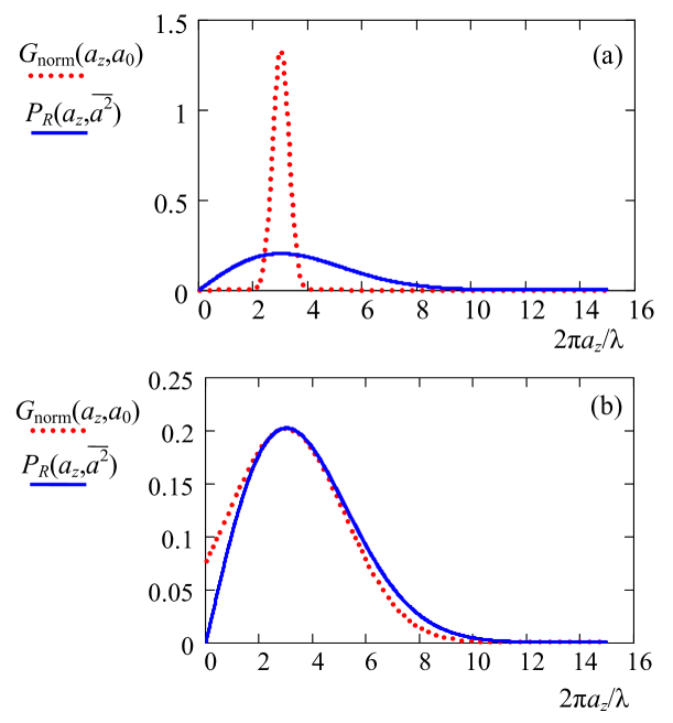
Figure 2: (color on line) The dependence of our distributions $G_{\text{norm}}\left(a,a_{0}\right)$ (dotted line in red) and Raylegh distribution (solid line in blue) on the amplitude of the displacement $a_{z}$. In our distribution variable $a$ is expressed as $a_{z}$, which have the same meaning as $a$ in Eq. (21). In both plots $a_{0}=\sqrt{\overline{a^{2}}}=3\lambda/2\pi$, which corresponds to $m_{0}=3$. Parameter $\sigma$ is 0.1 in (a), and 0.72 in (b).

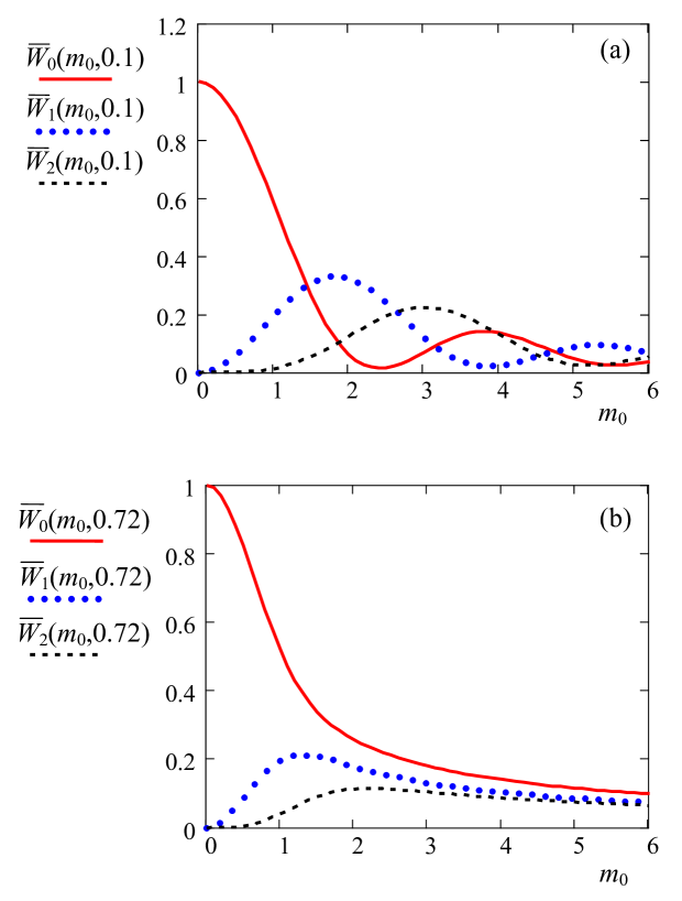
Figure 3: (color on line) Dependence of the intensity $\overline{W}_{n}\left(m_{0},\sigma\right)$ on $m_{0}$ for our model. Parameter $\sigma$ is 0.1 in (a) and 0.72 in (b). Solid line (in red) corresponds to $n=0$, dotted line (in blue) shows the dependence for $n=1$, and dashed line (in black) corresponds to $n=3$.

V Experiment

Our experimental setup is based on an ordinary Mössbauer spectrometer. The source, ⁵⁷Co:Rh, is mounted on the holder of the Mössbauer drive, which is used to Doppler-shift the frequency of the radiation of the source.

We carried out experiments with two differen absorbers. The first absorber was made of enriched K₄Fe(CN)${}_{6}\cdot 3$H₂O powder with effective thickness 13.2. It was mechanically pressed to the surface of the transducer. Therefore, in the experiments with powder the source was mounted above the absorber and the detector was placed below the absorber. This vertical geometry of the experiment allowed to consider a powder as a grained substance just freely jumping up and down under the influence of the vibrating transducer.

As a transducer we used in both experiments a polyvinylidene fluoride (PVDF) piezo polymer film (thickness 28 $\mu$m, model LDT0-28K, Measurement Specialties, Inc.). Several piezoelectric transducer constructions were tested to achieve the best performance. The best of them was a piece of 28 $\mu$m thick, 10$\times$12 mm polar PVDF film coupled to a plexiglas backing of $\sim$2 mm thickness with epoxy glue. The PVDF film transforms the sinusoidal signal from the radio-frequency (RF) generator into a uniform vibration of the absorber nuclei.

The second absorber was 25-$\mu$m-thick stainless-steel foil (from Alfa Aesar) with a natural abundance ($\sim$2.2%) of ⁵⁷Fe. Optical depth of the absorber is $T_{A}=5.18$. The stainless-steel foil is glued on the PVDF piezotransducer. Therefore, the experiments with stainless-steel foil were carried out in a standard horizontal geometry.

V.1 Powder absorber

Initially we supposed that powder absorber would behave as a sand placed on the vibrated transducer. Then, powder grains should randomly jump and fall down to the vibrated surface with phase depending on the size and weight of the grains. Therefore, we expected that single parent line should not split in sidebands, which must be strongly broadened due to the random motion of grains, and hence vibrational sidebands could give only a broadening of the wings of the absorption line. However, in a wide range of the vibration frequencies from 5 MHz to 45 MHz we observed the sidebands. We used the same voltage, 10V, supplied from RF generator, except for high frequencies (35 , 40, and 45 MHz). For them we elevated voltage up to 16V since the amplitudes of the sidebands significantly reduced with increase of the RF frequency and we could observe for high frequencies only first two sidebands $\omega_{S}\pm\Omega$ with very small intensities.

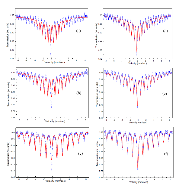
Figure 4: (color on line) Adsorption spectra of the powder absorber vibrated with frequency $\Omega$ equal to 7.5 MHz (a) and (d), 10 MHz (b) and (e), and 15 MHz (c) and (f). Dots are experimental data, solid line (in red) is the theoretical fitting to the Abragam model (a)-(c) and our model (d)-(f). For the Abragam model the modulation index $m_{0}=2\pi\sqrt{\overline{a^{2}}}/\lambda$ is 3.42 in (a), 3.66 in (b), and 3.39 in (c). For our model we obtained $m_{0}$, which is 5.6 in (d), 4.3 in (e), and 4.7 in (f).

The fitting of the experimental data to the theoretical models is shown in Fig. 4, where in (a)-(c) the Abragam model is used, while in (d)-(f) our model is applied to fit data. Abragam model gives bad fitting except frequencies $\Omega$ equal or higher than 35 MHz when we observed only three lines, i.e., the central component and two small sidebands. For frequencies below 35 MHz, especially the central component and components near to it are in a strong disagreement with the Abragam model. The spectra calculated according to our model agree well with experiment.

According to our model, for the same voltage from RF generator (10V), mean value of the modulation index $m_{0}$ takes maximum value $m_{0}=5.6$ for $\Omega=7.5$ MHz and then decreases with increase of the frequency $\Omega$. For example, for $\Omega=15$ MHz we have $m_{0}=4.7$, while for $\Omega=20$ MHz mean value of the modulation index drops almost two times, i.e., $m_{0}=2.6$. The smallest value of the modulation index $m_{0}=0.25$ was obtained for $\Omega=40$ MHz when the voltage was even elevated to 16V. Such a dependence of $m_{0}$ on the modulation frequency $\Omega$ could be explained by maximum efficiency of the process inducing mechanical vibrations of the powder near $\Omega=7.5$ MHz.

The best fitting of the experimental data to our theoretical predictions is obtained with $\sigma=0.85$, which corresponds to the value of the square root of variance $\sqrt{\delta a^{2}}$ equal to 85% of the mean amplitude $a_{0}$. This reflects a large spread of the amplitudes of the mechanical vibrations $a$ around $a_{0}$. Comparison of our distribution $G_{\text{norm}}(a,a_{0})$ with the Rayleigh distribution $P_{R}\left(a_{z},\overline{a^{2}}\right)$ for $m_{0}=5.6$ and $\sigma=0.85$ is shown in Fig. 5. Our distribution looks close to the continuous uniform distribution for the values of $a$ between 0 and $2\lambda$. Since our powder is hygroscopic, it does not behave as a dry sand. Such a powder can be compressed in a tablet-like substance, which shows small adhesion to the surface of the PVDF transducer. This could explain the coherent move of the powder grains. Their difference in size and orientation of the crystalline axis with respect to the direction of the displacement $z$ could explain almost continuous uniform distribution of the displacement amplitudes.

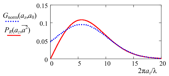
Figure 5: (color on line) The functional dependence of our distribution $G_{\text{norm}}\left(a,a_{0}\right)$ on the amplitude of the displacement $a_{z}$ for $m_{0}=5.6$ and $\sigma=0.85$ (dotted line in blue). The Rayleigh distribution for the value of $\sqrt{\overline{a^{2}}}=a_{0}$, where $a_{0}=m_{0}\lambda/2\pi$, is shown for comparison by the solid line (in red).

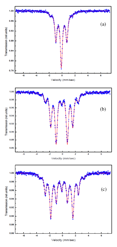
Figure 6: (color on line) Adsorption spectra for SS absorber vibrated with frequency 10 MHz. Dots are experimental data, solid line (in red) is the theoretical fitting to our model. Fitting parameters are $m_{0}=1.19$ and $\sigma=0.18$ in (a), $m_{0}=2.38$ and $\sigma=0.16$ in (b), and $m_{0}=3.01$ and $\sigma=0.16$ in (c).

V.2 Stainless steel absorber

The spectra obtained for the stainless steel absorber are quite different from those observed for the powder absorber. They demonstrated some features typical for the coherent model, see Fig. 6. However, these spectra could not be reasonably well described by the simple coherent model.

In Ref. Mkrtchyan79 it was assumed that some part of nuclei in the absorber vibrate coherently with the same amplitude, while another part of nuclei also take part in the coherent vibration, but for them the mean square displacement value changes from nucleus to nucleus. We could fit experimental data for SS absorber to the model Mkrtchyan79 , where experimental spectra are compared with theoretical predictions assuming a mixture (a simple sum with different weights) of the coherent and incoherent models. However, this method did not allow to obtain good fitting. Therefore, we decided to fit experimental spectra to our model. The results of fitting are shown in Fig. 6.

Figure 7: (color on line) Comparison of our distribution $G_{\text{norm}}\left(a,a_{0}\right)$ (dotted line in blue) with the Rayleigh distribution (solid line in red) for the modulation index $m_{0}=3.01$ and $\sigma=0.16$.

V.3 Model for SS foil vibration

The fitting allowed us to find the parameter $\sigma$. Figure 7 shows comparison of our distribution for this parameter with the Rayleigh distribution for the modulation index $m_{0}=3.01$. It is clear that for SS absorber the distribution of the displacement amplitude looks bell shape. Such a distribution gives a hint about a real distribution of the vibration amplitudes along the surface of the absorber. Before constructing this real distribution we give some arguments in support of the model.

PVDF film is glued on the solid plexiglas backing. Oscillating voltage forces the film to change its thickness making it thicker or narrower. We may assume that the lateral size of the film also oscillates. However, the solid backing resists the lateral changes of the film size. Therefore, we may assume that amplitude of the displacement is larger in the center of the film and smaller at the edges.

To avoid complications we model SS film as having a form of a disc with radius $r_{0}$. This disc vibrates such that the displacement has a maximum at the center and decreases to the edges. All elements of the disc vibrate with the same frequency and phase. We assume that the amplitudes of the vibrations are distributed according to a bell-shape function, slightly resembling $G_{\text{norm}}(a,a_{0})$, as

$$a_{z}(r)=a_{0}\cos\left(\xi\frac{\pi}{2}\frac{r}{r_{0}}\right),$$ (24)

where $a_{0}$ is a maximum amplitude at the disc center, $r$ is a distance from the center, and $\xi$ is a parameter, which specifies the difference between the amplitudes at the center, $a_{z}(0)=a_{0}$, and edges, $a_{z}(r_{0})=a_{0}\cos\left(\xi\pi/2\right)$. If $\xi\ll 1$, then this difference is small and the distribution is close to that when the amplitudes are uniform along the absorber. If $\xi=1$, then the amplitude at the edges of the disc are zero. In both cases the distribution is a bell shape as it is expected.

We assume that a beam of $\gamma$-radiation is transversely uniform and covers the hole disk. Actually, this is not the case. In reality we have to consider $2r_{0}$ as a diameter of the $\gamma$-beam, which is defined by the collimator aperture and the distance from the source to absorber. Then, the intensity of the transmitted radiation for the $n$th sideband is described by the integral over the area $S_{0}=\pi r_{0}^{2}$

$$\widetilde{W}_{n}(m_{0},r_{0},\xi)=\frac{2}{r_{0}^{2}}\int_{0}^{r_{0}}J_{n}^{2}\left[m_{0}\cos\left(\xi\frac{\pi}{2}\frac{r}{r_{0}}\right)\right]rdr,$$ (25)

which is normalized to $S_{0}$, where $m_{0}=2\pi a_{0}/\lambda$. Parameter $r_{0}$ can be excluded from the model if we introduce a variable $x=r/r_{0}$. Then, Eq. (25) is reduced to

$$\widetilde{W}_{n}(m_{0},\xi)=2\int_{0}^{1}J_{n}^{2}\left[m_{0}\cos\left(\xi\frac{\pi}{2}x\right)\right]xdx.$$ (26)

Thus, the parameter $\xi$ defines a measure of homogeneity of the vibration amplitudes across the beam of $\gamma$-radiation. If $\xi\rightarrow 0$, the vibration amplitudes are almost the same for all nuclei exposed to $\gamma$-radiation. If $\xi\rightarrow 1$, the amplitudes are very different. Our modeling assumption about the shape of the absorber is not important if $2r_{0}$ is smaller that the lateral dimensions of the absorber. In this case $2r_{0}$ means just the $\gamma$-beam diameter.

The dependence of the intensities of the spectral components $\widetilde{W}_{n}(m_{0},\xi)$ for $n=0$, $1$, and $2$ is shown in Fig. 8. For small $\xi$ ($\xi=0.1$) this dependence is close to that inherent to the coherent model since the vibration amplitudes of nuclei are almost the same. For the value $\xi$ ($\xi=0.95$) the dependence resembles the predictions of the Abragam model.

The similarity of the results originates from the similarity of the structure of the integrals in Eqs. (16) and (26) where the Bessel function is averaged with the function proportional to $a_{z}da_{z}$ in Eq. (16) and to $xdx$ in Eq. (26). Another common feature is that both distributions are centered at the value of the integration variable, which is zero, i.e., $a_{z}=0$ in Eq. (16) and $x=0$ ($r=0$) in Eq. (26). However, these distributions are very different in one important point. Rayleigh distribution is based on the assumption that the probability has maximum for zero displacement $a_{z}$. Our distribution assumes that the displacement amplitude has maximum value $\ a_{0}\neq 0$ when radius $r$, which is the averaging parameter, is zero.

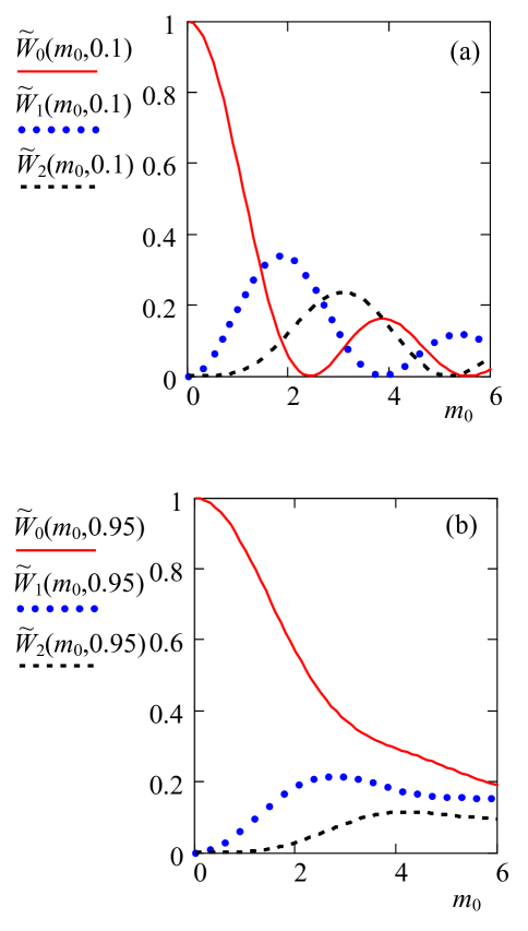
Figure 8: (color on line) Dependence of the intensity ${\widetilde{W}}_{n}\left(m_{0},\xi\right)$ on $m_{0}$ for the model of disc vibration. Parameter $\xi$ is 0.1 in (a) and 0.95 in (b). Solid line (in red) corresponds to $n=0$, dotted line (in blue) shows the dependence for $n=1$, and dashed line (in black) corresponds to $n=3$.

Experimental spectra are described much better by theoretical prediction, based on the disc model, compared with our first model. Therefore, we conclude that the disc model is more appropriate for description of the SS foil vibration. The fitting parameter $\xi$ is quite small. This means that dispersion of the displacements along the surface of the film is also small.

V.4 Absorber with a mask

We may assume that if the disc model is more adequate than other models, then following this model it would be possible to find experimental conditions when the vibration amplitudes of nuclei, exposed to gamma radiation, could be made even more homogeneous. ff we would increase the homogeneity, then the experimental spectra would be even more closer to those, which follow from the coherent model.

According to the disk model the simplest way to increase the homogeneity of the displacement is to remove the contribution of nuclei located far from the absorber center. This could be done by placing a mask with a small hole in the front of absorber and locate the mask such that the hole coincides with the absorber center. Then, $\gamma$-radiation will propagate only through the hole, and only nuclei, located behind the hole will interact with $\gamma$-radiation.

To make sure that our assumptions are correct, we measured several spectra with different diameter of the hole. According to our expectations the spectra must change with the change of the size of the hole.

Figure 9: (color on line) Adsorption spectra for SS absorber obtained with the mask. Diameter of the hole in the mask is 2.45 mm in (a), 1.7 mm in (b), and 1.1 mm in (c). The absorber is vibrated with frequency 10.7 MHz. Dots are experimental data, solid line (in red) is the theoretical fitting to the disk model. The values of the modulation index $m_{0}$ and parameter $\xi$ are 1.85 and 0.27 in (a), 2.08 and 0.25 in (b), and 2.68 and 0.21 in (c), respectively.

The absorption spectra of the absorber with the mask are shown in Fig. 9. Diameter of the mask was varied from 2.45 mm to 1.1 mm. These spectra are obtained for the same frequency and voltage of RF generator. In the coherent model the central component becomes zero for the modulation index $m=2.4$. We suppose that spectra in Fig. 9 are obtained with the modulation index quite close to this value. Therefore, the observed lessening of the central component of the absorption spectra with diminution of the mask diameter proves that scattering of the vibration amplitudes of nuclei, exposed to $\gamma$-radiation, becomes smaller with decrease of the size of the hole. At the same time the intensities of the sidebands increase with diminution of the hole diameter.

For the smallest hole, the disc model gives the maximum value of the vibration amplitude $a_{0}=36.7$ pm at the disc center. The scattering parameter $\xi=0.21$ for this hole is small. Therefore, the amplitude at the disc edge $a_{z}(r_{0})=a_{0}\cos(\xi\pi/2)$ is 34.7 pm, which differs from $a_{0}$ only by 2 pm. This 5$\%$ difference gives the accuracy of the displacement measurement with the smallest hole.

By this mask with the smallest hole (1.1 mm) we scanned the surface of the absorber. The obtained spectra are shown in Fig. 10. Since the spectra obtained with the mask having the smallest hole are very close to that predicted by the coherent model, we expect that such a scanning is capable to provide the information about distribution of the vibration amplitudes along the surface of the absorber. We obtained the following results. When the hole coincides with the center of the absorber we have the splitting of the parent line into sidebands, which corresponds to the modulation index $m=2.67$, see Fig. 10(a). Positions of the hole slightly below the center and shifted to the left in (c) and right in (d) give reduction of the modulation index to the values $m=2.37$ in (c) and $m=2.35$ in (d). Since these values are close to each other we may conclude that transverse shift (left/right) of the hole does not show appreciable change of the vibration amplitude. If we move the hole further down from the center, the value of the modulation index reduces to $m=1.74$, see Fig. 10(b).

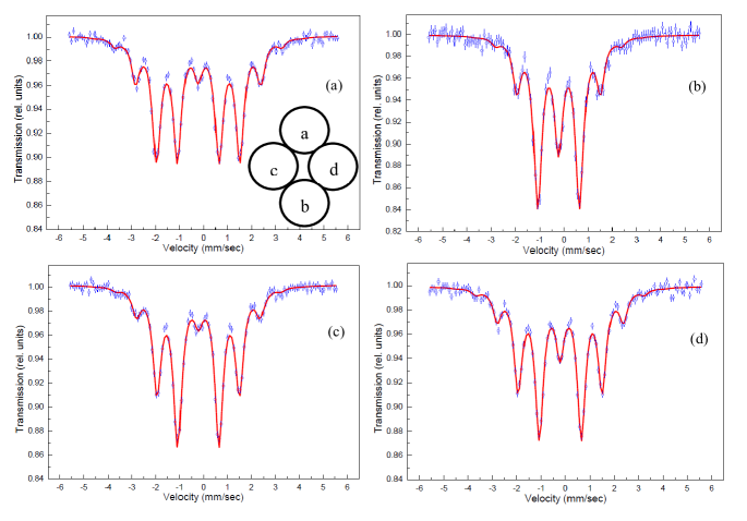
Figure 10: (color on line) Adsorption spectra for SS absorber obtained with the mask. The hole diameter in the mask is 1.1 mm. The hole position on the absorber is shown in the inset in (a) by black circles. Position of the upper circle coincides with the absorber center [spectrum (a)]. Other circles are moved away to the bottom [spectrum (b)], to the left and bottom [spectrum (c)], and to the right and bottom [spectrum (d)]. The absorber is vibrated with frequency 10 MHz. The driving voltage is $V=10.7$ V. Dots are experimental data, solid line (in red) is the theoretical fitting. The fitting parameters are $m_{0}=2.67$ and $\xi=0.18$ in (a), $m_{0}=1.74$ and $\xi=0.24$ in (b), $m_{0}=2.37$ and $\xi=0.18$ in (c), and $m_{0}=2.35$ and $\xi=0.27$ in (b).

VI Discussion

Our experimental results, obtained for SS foil, give a strong hint at the presence of longitudinal distribution of the displacement amplitudes on the surface of the absorber, while in the transverse direction the amplitudes are more homogeneous. Since PVDF film is drawn and polarized during its fabrication, it is natural to expect the difference of the displacements in longitudinal and transverse directions. Long polymer chains aligned along a particular direction give the origin to this asymmetry. Therefore, we assume that our disc model cannot describe perfectly all the details of the vibration of the PVDF film together with SS foil. However this model is good to describe the experiments with the mask having a round hole. We plan to develop a strip model of the vibration, which could be more adequate. Future experiments with a mask, whose small hole is scanned over the surface of the absorber, could provide topographical information about amplitude distribution over the sample surface. We expect that this information could help to construct such a model.

As regards the powder absorber, we could screen the powder through a set of grids to make the powder grains almost of the same size. We expect that experiments with such a homogeneous powder could elucidate the origin of the spectrum behavior of the vibrated powder.

VII Conclusion

We studied the transformation of Mössbauer single parent line of the vibrated absorber into a reduced intensity central line accompanied by many sidebands. The intensities of the sidebands contain information about the amplitudes of the mechanical vibrations and their distribution along the surface of the absorber. Two absorbers, powder and SS foil, are experimentally studied. The experimental spectra are fitted to the model with two parameters, i.e., the mean amplitude of the vibrations and their deviation, which is defined in a percentage of the mean amplitude. This model allows to conclude that the distribution of the displacements in powder absorber is close to the continuous uniform distribution with large scattering of the amplitudes, while for SS foil it is bell shaped with small scattering of the amplitudes. We proposed a distribution of the displacements in SS foil, which is related to the geometrical distribution of displacements along the surface of the foil. To verify our proposal we measured the spectra of the vibrated SS foil placing a mask with a small hole in it before the absorber. When the diameter of the hole in the mask is 1 mm, the displacements become almost uniform with 5$\%$ scattering around maximum value of the displacement. Therefore, the spectra can be described by the coherent model. This allows to measure the displacements along the surface of the vibrated foil with the accuracy 2 pm. We expect that our finding will open a way for a new kind of spectroscopical measurements of extra small displacements.

VIII Acknowledgements

This work was partially funded by the Russian Foundation for Basic Research (Grant No. 15-02-09039-a), the Program of Competitive Growth of Kazan Federal University, funded by the Russian Government, and the RAS Presidium Program “Fundamental optical spectroscopy and its applications.”

References

- (1) S. W. Hell, Nature Methods 6, 24 (2009).
- (2) S. L. Ruby, D. I. Bolef, Phys. Rev. Lett. 5, 5 (1960).
- (3) T. E. Cranshaw and P. Reivari, Proc. Phys. Soc. 90, 1059 (1967).
- (4) J. Mishroy and D. I. Bolef, Mössbauer Effect Methodology, edited by I. J. Gruverman (Plenum Press, Inc. New York, 1968), Vol. 4, P. 13-35.
- (5) G. Kornfeld, Phys. Rev. 177, 494 (1969).
- (6) C. L. Chien, J. C. Walker, Phys. Rev. B 13, 1876 (1976).
- (7) A. R. Mkrtchyan, A. R. Arakelyan, G. A. Arutyunyan, and L. A. Kocharyan, Pis’ma Zh. Eksp. Teor. Fiz. Pisma 26, 599 (1977) [JETP Lett. 26, 449 (1977).
- (8) G. J. Perlow, Phys. Rev. Lett. 40, 896 (1978).
- (9) J. E. Monahan, and G. J. Perlow, Phys. Rev. A 20, 1499 (1979).
- (10) A. R. Mkrtchyan, G. A. Arutyunyan, A. R. Arakelyan, and R. G. Gabrielyan, Phys. Stat. Sol. b 92, 23 (1979).
- (11) S. L. Popov, G. V. Smirnov, and Yu. V. Shvyd’ko, JETP Lett. 49, 747 (1989).
- (12) Yu. V. Shvyd’ko and G. V. Smirnov, J. Phys.: Condens. Matter 4, 2663 (1992).
- (13) F. J. Lynch, R. E. Holland, and M. Hamermesh, Phys. Rev. 120, 513 (1960).
- (14) F. Vagizov, V. Antonov, Y. V. Radeonychev, R. N. Shakhmuratov, and O. Kocharovskaya, Nature 508, 80 (2014).
- (15) R. N. Shakhmuratov, F. G. Vagizov, V. A. Antonov, Y. V. Radeonychev, M. O. Scully, and O. Kocharovskaya, Phys. Rev. A 92, 023836 (2015).
- (16) A. Abragam, Compt. Rend. 250, 4334 (1960).
- (17) L. T. Tsankov, J. Phys. A: Math. Gen. 14, 275 (1981).
- (18) A. Gupta, Phys. Rev. B 24, 2362 (1981).
- (19) P. Helisto, E. Ikonen, and T. Katila, Hyperfine Interactions 29, 1563 (1986).
- (20) F. Vagizov, R. Shakhmuratov, and E. Sadykov, Phys. Status Solidi B 252, 469 (2015).
- (21) R. N. Shakhmuratov, F. G. Vagizov, M. O. Scully, and O. Kocharovskaya, Phys. Rev. A 94, 043849 (2016).
- (22) R. N. Shakhmuratov and A. Szabo, Phys. Rev. A 58, 3099 (1998).