Modeling of cyclic creep in the finite strain range using a nested multiplicative split

Abstract.

A new phenomenological model of cyclic creep is proposed which is suitable for applications involving finite creep deformations of the material. The model accounts for the the effect of the transient increase of the creep strain rate upon the load reversal. In order to extend the applicability range of the model, the creep process is fully coupled to the classical Kachanov-Rabonov damage evolution. As a result, the proposed model describes all the three stages of creep. Large strain kinematics is described in a geometrically exact manner using the assumption of a nested multiplicative split, originally proposed by Lion for finite strain plasticity. The model is thermodynamically admissible, objective, and w-invariant. Implicit time integration of the proposed evolution equations is discussed. The corresponding numerical algorithm is implemented into the commercial FEM code MSC.MARC. Using this code, the model is validated using real experimental data on cyclic torsion of a thick-walled tubular specimen made of the D16T aluminium alloy. The numerically computed stress distribution exhibits a “skeletal point” within the specimen.

1. Introduction

In numerous industrial applications, hight-temperature metallic structural components are loaded by large stresses. Under such conditions their long term behaviour depends on the creep-related effects, such as the accumulation of irreversible creep deformations, redistribution of stresses, creep-induced anisotropy and creep damage [6, 3]. In the current study, the classical phenomenological approach to the modeling of creep is developed within the framework of irreversible thermodynamics.

In the static case when applied stresses and temperature are constant, one usually identifies three stages of creep: primary stage (characterized by transient or non-stationary response), secondary stage (steady-state creep) and tertiary stage (damage-dominated creep). The creep rate typically reduces during the transition from the primary creep to the steady-state creep. It is commonly accepted that this creep rate reduction is caused by the material hardening, whereas the steady-state phase is characterized by a balance between hardening and recovery processes [4]. Apart from the primary creep under constant stress, the transient creep phenomenon occurs also immediately after rapid changes of applied stresses. In particular, a non-stationary creep is observed if the applied stresses are reversed. This transient process is characterized on the macroscopic level by a relatively short period of an increased creep rate. During the holding time after the stress reversal, this transient process is followed by the saturation to a reduced steady-state creep rate (cf., for example, Chapter 2.3 of Ref. [3]). The accelerated creep strain rate after the stress reversal ($\sigma\mapsto-\sigma$) was experimentally observed in many studies (see, among others, [36, 10, 37]). Another macroscopic manifestation of a non-stationary creep is as follows: After an abrupt drop of the applied stress from $\sigma_{1}$ to $\sigma_{2}$ ($\sigma_{1}>\sigma_{2}$) the resulting creep rate is lower than the steady-state creep rate observed in the material under $\sigma_{2}$. At the same time, after an abrupt stress jump from $\sigma_{2}$ to $\sigma_{1}$, the resulting creep rate is higher than the steady-state creep rate corresponding to the constant stress level $\sigma_{2}$ [54]. The creep recovery upon the removal of applied stresses [3] is another transient effect of this kind.

The above mentioned effects indicate that the creep is a loading-history dependent anisotropic phenomenon. An accurate description of the transient creep response of the material is necessary for the correct analysis of high-temperature industrial components operating under cyclic loads [17]. The effect of the process-induced anisotropy is less evident in case of a strain-controlled loading, but, nevertheless, it still has to be accounted for (cf. [42, 35, 25]). Let us briefly discuss the main phenomenological approaches to cyclic creep. The most simple macroscopic description of the transient stage is provided by the concept of isotropic creep-hardening [6]. Unfortunately, as one may expect, the simple isotropy assumption is not sufficient in many practical cases [16, 32, 36]. One of the most popular macroscopic approaches to the creep-induced anisotropy is based on the concept of kinematic hardening, which was borrowed from the phenomenological plasticity. Within this concept, backstresses are introduced as a measure of the accumulated anisotropy . Although the concept of backstresses is nowadays wide spread, there are different micromechanical interpretations in case of polycristalline materials. One may assume that some backstresses represent a resistance to dislocation motion caused by pile-ups of dislocations [11, 57] (atomistic scale), while other backstresses represent an internal residual stress field caused by plastic strain incompatibilities between grains (mesoscopic scale) [15]. In either way, backstresses superimpose with the applied mechanical stresses such that the creep is governed by the effective stress, computed according to the formula

$$\text{effective stress}=\text{mechanical stress}-\text{backstress}.$$

Following this concept, the anisotropic creep is assumed to be governed by the effective stresses [30, 28, 22, 24]. In particular, the assumption is made that the creep strain rate is coaxial to the deviatoric effective stresses, not to the deviatoric part of the stresses itself [14].

The evolution of the backstress $X$ can be described in a hardening/recovery format (see Section 2), where the hardening term represents the microstructural changes associated with the material strengthening and the recovery term is typically related to the softening of the material

$$\dot{X}=\dot{X}|_{\text{hardening}}-\dot{X}|_{\text{recovery}}.$$

The hardening term is usually strain controlled; therefore it is assumed as a homogeneous function of the creep strain rate $\dot{\varepsilon}_{\text{cr}}$

$$\dot{X}|_{\text{hardening}}(\alpha\dot{\varepsilon}_{\text{cr}})=\alpha\dot{X}|_{\text{hardening}}(\dot{\varepsilon}_{\text{cr}})\quad\text{for all}\ \alpha\geq 0.$$

Dynamic recovery of the backstress implies strain-controlled creep hardening (e.g. Armstrong-Frederick-like behaviour, or, equivalently, endochronic Maxwell-like behaviour)

$$\dot{X}|_{\text{recovery}}=\|\dot{\varepsilon}_{\text{cr}}\|{F}(X),$$

where $F(X)$ is a suitable function of the backstress $X$ and $\|\dot{\varepsilon}_{\text{cr}}\|$ is a norm of the creep strain rate. The dynamic recovery format was used, among others, in [34, 25]. This type of material behaviour is also known as a strain-activated recovery. Alternatively, one may assume the so-called static recovery, which implies time-controlled evolution (e.g. Maxwell-like behaviour)

$$\dot{X}|_{\text{recovery}}=\dot{X}|_{\text{recovery}}(X).$$

Since this process is partially driven by the diffusion, it is highly temperature dependent; for that reason static recovery is also known as a temperature-controlled recovery. The static recovery format was implemented in [30, 52, 27, 22, 14, 57]. Backstress-based creep models combining both static and dynamic recovery are also known (see eq. (8) in [33], eq. (62) in [22] or eq. (3) in [59]). Such a combined static/dynamic approach is utilized in the current study as well.

The basic hardening/recovery format mentioned above can be further specified in a number of ways. The evolution equations proposed in [27] are motivated by microstructural information, namely, by experimental measurements of the (average) dislocation cell size. An additional constitutive assumption was used in [14] to capture the history-dependent material response: the stress response is assumed to depend on the maximum value of the backstress, achieved in the previous history. In some studies, the saturation level for backstresses depends on the applied stresses [30, 14, 17]. In [57, 58] the backstresses are not necessarily deviatoric; the hydrostatic component of the backstrasses is relevant for pressure-sensitive materials.

The safety analysis of industrial components is mostly concerned with small strain creep. Comprehensive reviews of different creep hardening rules in the small strain context can be found in [9, 38]. At the same time, analysis of accident scenarios may involve finite strains as well; moreover, a number of metal forming applications involve creep processes in the finite strain range. Unfortunately, there is only a few publications devoted to the finite strain creep analysis (see, among others, [8, 27]). The aim of the current paper is to fill this gap; we apply the state of the art methodology of anisotropic multiplicative plasticity to the specific problems of creep mechanics. Here we choose the multiplicative framework since it has numerous advantages over alternative approaches [49]. Following [29], the classical decomposition of the deformation gradient into inelastic (creep) and elastic parts is now supplemented by a nested multiplicative split of the inelastic part into some dissipative and conservative parts. This decomposition allows one to incorporate the nonlinear kinematic hardening in a thermodynamically consistent way (see [20, 45, 60, 43, 7, 23] among others).

The paper is organized as follows. In Section 2 the constitutive equations of the developed creep model are presented. In Section 3 the numerical implementation of the proposed model is discussed. In Section 4 the model is validated using the experimental data on the torsion of a thick-walled tubular sample made of D16T aluminum alloy.

A coordinate-free tensor formalism (direct tensor notation) is used in the current study. Second- and fourth-rank tensors in $\mathbb{R}^{3}$ are denoted by bold symbols. Notations $\text{tr}(\cdot)$, $(\cdot)^{\text{D}}$, $(\cdot)^{\text{T}}$, $(\cdot)^{\text{-T}}$, $\det(\cdot)$ stand for the trace, deviatoric part, transposition, inverse of transposed, and determinant, respectively. The symmetric part, scalar product of two second-rank tensors (double contraction), the Frobenius norm, and the unimodular part are defined as follows

$$\text{sym}(\mathbf{A}):=\frac{1}{2}(\mathbf{A}+\mathbf{A}^{\text{T}}),\quad\mathbf{A}:\mathbf{B}\ :=\text{tr}(\mathbf{A}\ \mathbf{B}^{\text{T}}),\quad\|\mathbf{A}\|:=\sqrt{\mathbf{A}:\mathbf{A}},\quad\overline{\mathbf{A}}:=(\det(\mathbf{A}))^{-1/3}\ \mathbf{A}.$$ (1)

Suffixes $(\cdot)_{\text{el}}$, $(\cdot)_{\text{cr}}$, $(\cdot)_{\text{ii}}$, and $(\cdot)_{\text{ie}}$ stand for “elastic”, “creep”, “inelastic-inelastic”, “inelastic-elastic”. Since the presentation is coordinate free, these suffixes can not be mistaken for tensor coordinates.

2. Material model of anisotropic creep with isotropic damage

The constitutive equations of creep will be combined with the classical Kachanov-Rabotnov approach to creep damage. Toward that end we introduce the Rabotnov damage variable $\omega\in[0,1]$. Schematically, $\omega=0$ corresponds to the intact material and $\omega=1$ characterizes a fully destroyed material with a macroscopic crack [21, 41, 31].

2.1. Small strain case

\psfrag{A}[m][1][0]{$\boldsymbol{\varepsilon}_{\text{cr}}$}\psfrag{B}[m][1][0]{$\boldsymbol{\varepsilon}_{\text{e}}$}\psfrag{C}[m][1][0]{$\boldsymbol{\varepsilon}$}\psfrag{D}[m][1][0]{substructure}\psfrag{E}[m][1][0]{$\boldsymbol{\varepsilon}_{\text{ii}}$}\psfrag{F}[m][1][0]{$\boldsymbol{\varepsilon}_{\text{ie}}$}\psfrag{Q}[m][1][0]{a)}\psfrag{R}[m][1][0]{b)}\psfrag{G}[m][1][0]{$\varkappa_{\text{stat}}$}\psfrag{M}[m][1][0]{$\varkappa_{\text{dynam}}$}\psfrag{H}[m][1][0]{$c$}\psfrag{K}[m][1][0]{$\alpha^{\lambda}_{1},\alpha^{\lambda}_{2},\alpha,...$}\psfrag{L}[m][1][0]{$k,\mu$}\includegraphics{fig1.eps}

Figure 1. Rheological model of creep with nonlinear kinematic hardening, which includes static and dynamic recovery: decomposition of the infinitesimal strain (left) and introduced material parameters (right).

We start with a small strain version of the material model, which is extremely simple since geometric nonlinearities are neglected. To visualize the main modeling assumptions we employ the rheological interpretation shown in Fig. 1(left). The rheological model consists of two generalized Maxwell bodies (accounting for static and dynamic recovery), a Hooke body and a modified Newton body. The overall infinitesimal strain tensor $\boldsymbol{\varepsilon}$ is decomposed additively into the creep strain $\boldsymbol{\varepsilon}_{\text{cr}}$ and the elastic strain $\boldsymbol{\varepsilon}_{\text{e}}$. The creep strain itself is decomposed into the dissipative part $\boldsymbol{\varepsilon}_{\text{ii}}$ and the conservative part $\boldsymbol{\varepsilon}_{\text{ie}}$

$$\boldsymbol{\varepsilon}=\boldsymbol{\varepsilon}_{\text{cr}}+\boldsymbol{\varepsilon}_{\text{e}},\quad\boldsymbol{\varepsilon}_{\text{cr}}=\boldsymbol{\varepsilon}_{\text{ii}}+\boldsymbol{\varepsilon}_{\text{ie}}.$$ (2)

Using these strain variables we define the Helmholz free energy per unit mass

$$\psi=\psi(\boldsymbol{\varepsilon}_{\text{e}},\boldsymbol{\varepsilon}_{\text{ie}},\omega)=\psi_{\text{el}}(\boldsymbol{\varepsilon}_{\text{e}},\omega)+\psi_{\text{kin}}(\boldsymbol{\varepsilon}_{\text{ie}},\omega),$$ (3)

where $\psi_{\text{el}}(\boldsymbol{\varepsilon}_{\text{e}},\omega)$ is the energy storage due to the macroscopic elastic deformations of the crystal lattice and $\psi_{\text{kin}}(\boldsymbol{\varepsilon}_{\text{ie}},\omega)$ is the part of the energy stored in the defects of the crystal structure, associated with the kinematic hardening. The stress tensor $\boldsymbol{\sigma}$ and the backstress tensor $\boldsymbol{x}$ are then computed through

$$\boldsymbol{\sigma}=\rho\frac{\displaystyle\partial\psi_{\text{el}}(\boldsymbol{\varepsilon}_{\text{e}},\omega)}{\displaystyle\partial\boldsymbol{\varepsilon}_{\text{e}}},\quad\boldsymbol{x}=\rho\frac{\displaystyle\partial\psi_{\text{kin}}(\boldsymbol{\varepsilon}_{\text{ie}},\omega)}{\displaystyle\partial\boldsymbol{\varepsilon}_{\text{ie}}},$$ (4)

where $\rho$ is the mass density. The formulation of the model may employ various assumptions governing the free energy; however, to be definite, we use here the following quadratic strain energy function

$$\rho\psi_{\text{el}}(\boldsymbol{\varepsilon}_{\text{e}},\omega)=(1-\omega)\frac{k}{2}(\text{tr}\boldsymbol{\varepsilon}_{\text{e}})^{2}+(1-\omega)\mu\boldsymbol{\varepsilon}_{\text{e}}^{\text{D}}:\boldsymbol{\varepsilon}_{\text{e}}^{\text{D}},\quad\rho\psi_{\text{kin}}(\boldsymbol{\varepsilon}_{\text{ie}},\omega)=(1-\omega)\frac{c}{2}\boldsymbol{\varepsilon}_{\text{ie}}^{\text{D}}:\boldsymbol{\varepsilon}_{\text{ie}}^{\text{D}},$$ (5)

where $k$, $\mu$, and $c$ are material parameters characterizing the intact material. Substituting this into (4) we arrive at

$$\boldsymbol{\sigma}=k\ (1-\omega)\ \text{tr}(\boldsymbol{\varepsilon}_{\text{e}})\boldsymbol{1}+2\mu(1-\omega)\ \boldsymbol{\varepsilon}_{\text{e}}^{\text{D}},\quad\boldsymbol{x}=c(1-\omega)\ \boldsymbol{\varepsilon}_{\text{ie}}^{\text{D}},$$ (6)

where $\boldsymbol{1}$ is the second-rank identity tensor. According to (6), both the macroscopic elastic properties (bulk and shear moduli $k$ and $\mu$) and the elastic properties of the substructure (shear modulus of substructure $c$) deteriorate with damage. The effective stress is defined through

$$\boldsymbol{\sigma}_{\text{eff}}:=\boldsymbol{\sigma}-\boldsymbol{x}.$$ (7)

We assume that the effective stress $\boldsymbol{\sigma}_{\text{eff}}$ is the driving force of the global creep process. The framework which will be developed in the current study allows the creep strain rate to be an arbitrary isotropic function of the effective stress. However, for simplicity, we will restrict our attention to incompressible creep flow. In order to be more specific, we need the following preparations. First, let $\mathbf{A}$ be an arbitrary symmetric second-rank tensor. Its regularized maximum eigenvalue $\sigma_{\text{reg max}}(\mathbf{A})$ is defined through the formula

$$\sigma_{\text{reg max}}(\mathbf{A}):=(\langle a_{1}\rangle^{R}+\langle a_{2}\rangle^{R}+\langle a_{3}\rangle^{R})^{1/R},\quad\{a_{1},a_{2},a_{3}\}:=\text{eigenvalues of}\ \mathbf{A},$$ (8)

where $\langle x\rangle:=\max(0,x)$; $R>1$ is a regularization parameter. Next, two stress invariants (equivalent stresses) are defined in the following way

$$\sigma^{\lambda}_{\text{eq}}:=\alpha^{\lambda}_{1}\sigma_{\text{reg max}}(\boldsymbol{\sigma}_{\text{eff}})+\alpha^{\lambda}_{2}\ \sqrt{\frac{3}{2}}\ \|\boldsymbol{\sigma}^{\text{D}}_{\text{eff}}\|+(1-\alpha^{\lambda}_{1}-\alpha^{\lambda}_{2})\ \text{tr}(\boldsymbol{\sigma}_{\text{eff}}),$$ (9)

$$\sigma_{\text{eq}}:=\alpha\ \frac{3}{2}\ \sigma_{\text{reg max}}(\boldsymbol{\sigma}^{\text{D}}_{\text{eff}})+(1-\alpha)\ \sqrt{\frac{3}{2}}\ \|\boldsymbol{\sigma}^{\text{D}}_{\text{eff}}\|,$$ (10)

where $\alpha^{\lambda}_{1},\alpha^{\lambda}_{2},\alpha\geq 0$ are constant weighting factors. Note that these function are homogeneous functions of $\boldsymbol{\sigma}_{\text{eff}}$ of degree one. Using these, we postulate the flow rule in the form

$$\dot{\boldsymbol{\varepsilon}}_{\text{cr}}=\lambda(\sigma^{\lambda}_{\text{eq}},\omega)\frac{\partial\sigma_{\text{eq}}}{\partial\boldsymbol{\sigma}_{\text{eff}}},$$ (11)

where $\lambda(\sigma^{\lambda}_{\text{eq}},\omega)$ is a suitable function of the equivalent stress and damage $\omega$.

Remark 1. According to (11), the multiplier $\lambda(\sigma^{\lambda}_{\text{eq}},\omega)$ controls the intensity of the creep flow and $\frac{\displaystyle\partial\sigma_{\text{eq}}}{\displaystyle\partial\boldsymbol{\sigma}_{\text{eff}}}$ gives its direction. In fact, the flow rule (11) is based on the assumption that there is a creep flow potential. This assumption is quite common in the creep mechanics, even dealing with anisotropic materials [53]. $\Box$

Following the classical Kachanov-Rabotnov approach we postulate

$$\lambda(\sigma^{\lambda}_{\text{eq}},\omega)=(1-\omega)^{-m}\ \lambda_{\text{undamaged}}(\sigma^{\lambda}_{\text{eq}}),$$ (12)

where $m$ is a material parameter and $\lambda_{\text{undamaged}}(\sigma^{\lambda}_{\text{eq}})$ is the creep strain rate of the undamaged material. In general, any non-negative and smooth function $\lambda_{\text{undamaged}}(\sigma^{\lambda}_{\text{eq}})$ can be used if the natural restriction $\lambda_{\text{undamaged}}|_{\sigma^{\lambda}_{\text{eq}}=0}=0$ is satisifed. The following monotonic functions of $\sigma^{\lambda}_{\text{eq}}$ are frequently used in the phenomenological creep modeling (see, for example, [3])

$$\lambda_{\text{undamaged}}(\sigma^{\lambda}_{\text{eq}})=A(\sigma^{\lambda}_{\text{eq}}/f_{0})^{n},\quad f_{0}:=1\text{MPa},$$ (13)

$$\lambda_{\text{undamaged}}(\sigma^{\lambda}_{\text{eq}})=A(\exp(\sigma^{\lambda}_{\text{eq}}/\sigma_{0})-1),$$ (14)

$$\lambda_{\text{undamaged}}(\sigma^{\lambda}_{\text{eq}})=A\sinh(\sigma^{\lambda}_{\text{eq}}/\sigma_{0}),$$ (15)

$$\lambda_{\text{undamaged}}(\sigma^{\lambda}_{\text{eq}})=A_{1}(\sigma^{\lambda}_{\text{eq}}/f_{0})^{n_{1}}+A_{2}(\sigma^{\lambda}_{\text{eq}}/f_{0})^{n_{2}},\quad f_{0}:=1\text{MPa},$$ (16)

$$\lambda_{\text{undamaged}}(\sigma^{\lambda}_{\text{eq}})=A\big{(}\sinh(\sigma^{\lambda}_{\text{eq}}/\sigma_{0})\big{)}^{n},$$ (17)

where $A>0$, $A_{1}>0$, $A_{2}>0$, $\sigma_{0}>0$, $n\geq 1$, $n_{1}\geq 1$, $n_{2}\geq 1$ are material parameters.

Next, we assume that the backstress $\mathbf{x}$ is the driving force for the dissipative processes on the substructural level. In particular, the saturation of the kinematic hardening is described using the following flow rule

$$\dot{\boldsymbol{\varepsilon}}_{\text{ii}}=\varkappa_{\text{dynam}}\ \|\dot{\boldsymbol{\varepsilon}}_{\text{cr}}\|\ \mathbf{x}^{\text{D}}+\varkappa_{\text{stat}}\ \mathbf{x}^{\text{D}},$$ (18)

where $\varkappa_{\text{dynam}}\geq 0$ and $\varkappa_{\text{stat}}\geq 0$ are the parameters of dynamic and static recovery. Note that (18) and the corresponding material parameters are not influenced by damage. This is a strong simplifying assumption, but, as will be clear from the model validation (cf. Section 4), it yields good results.

Remark 2. The dynamic recovery term $\varkappa_{\text{dynam}}\ \|\dot{\boldsymbol{\varepsilon}}_{\text{cr}}\|\ \mathbf{x}$ is needed to capture the following important effect, observed in experiments on real materials: the higher the applied stress is, the shorter the transient stage [31]. Indeed, for high applied stress the creep rate is high thus leading to the fast saturation of $\mathbf{x}$. On the other hand, the dynamic term alone may be not enough to obtain a plausible mechanical response. In particular, the creep models with kinematic hardening without static recovery are prone to the following unphysical behaviour under static loading conditions: If the applied stress $\sigma$ is smaller than the saturation level for the backstress $\mathbf{x}$, then after a certain holding time the backstress equilibrates the applied stress and the creep rate becomes exactly zero. In order to prevent such unrealistic behaviour, the static recovery term $\varkappa_{\text{stat}}\ \mathbf{x}$ is introduced in (18). One important implication of the static recovery is that the deformation-induced backstresses relax even if the creep strain is frozen: $\mathbf{x}\rightarrow\mathbf{0}$ as $t\rightarrow\infty$ and $\dot{\boldsymbol{\varepsilon}}_{\text{cr}}=\mathbf{0}$. $\Box$

Remark 3. In this study we assume for simplicity $\varkappa_{\text{dynam}}=const$, which is sufficient for our goals. However, in some materials the saturation level of the backstresses is nearly proportional to the applied stresses. In order to capture this effect, one may consider $\varkappa$ to be a (positive) function of the applied stress $\boldsymbol{\sigma}$. $\Box$

Analogously to (9), to render the evolution of the damage variable $\omega$ we introduce a damage-related equivalent stress

$$\sigma^{\omega}_{\text{eq}}:=\alpha^{\omega}_{1}\sigma_{\text{reg max}}(\boldsymbol{\sigma}_{\text{eff}})+\alpha^{\omega}_{2}\ \sqrt{\frac{3}{2}}\ \|\boldsymbol{\sigma}^{\text{D}}_{\text{eff}}\|+(1-\alpha^{\omega}_{1}-\alpha^{\omega}_{2})\ \text{tr}(\boldsymbol{\sigma}_{\text{eff}}),\quad$$ (19)

where $\alpha^{\omega}_{1}\geq 0$ and $\alpha^{\omega}_{2}\geq 0$ are material constants. Then the damage evolution is given by the classical Kachanov-Rabotnov relation

$$\dot{\omega}=B(1-\omega)^{-l}(\sigma^{\omega}_{\text{eq}})^{k},$$ (20)

where $B$, $k$, and $l$ are material parameters.

Finally, in order to close the system of constitutive equations we put the following initial conditions

$$\boldsymbol{\varepsilon}_{\text{cr}}|_{t=0}=\boldsymbol{\varepsilon}^{0}_{\text{cr}},\quad\boldsymbol{\varepsilon}_{\text{ii}}|_{t=0}=\boldsymbol{\varepsilon}^{0}_{\text{ii}},\quad\omega|_{t=0}=\omega^{0}.$$ (21)

In general, the initial values $\boldsymbol{\varepsilon}^{0}_{\text{cr}}$ and $\boldsymbol{\varepsilon}^{0}_{\text{ii}}$ can be seen as additional material parameters, which characterize the material at $t=0$. Observe that the introduced material parameters can be interpreted in terms of the rheological model, as shown in Fig. 1(right).

2.2. Generalization to finite strains

\psfrag{A}[m][1][0]{${\mathbf{F}}_{\text{cr}}$}\psfrag{B}[m][1][0]{${\mathbf{F}}_{\text{e}}$}\psfrag{C}[m][1][0]{${\mathbf{F}}$}\psfrag{D}[m][1][0]{substructure}\psfrag{E}[m][1][0]{${\mathbf{F}}_{\text{ii}}$}\psfrag{F}[m][1][0]{${\mathbf{F}}_{\text{ie}}$}\psfrag{Q}[m][1][0]{a)}\psfrag{R}[m][1][0]{b)}\psfrag{I}[m][1][0]{$\tilde{\mathcal{K}}$}\psfrag{J}[m][1][0]{$\check{\mathcal{K}}$}\psfrag{K}[m][1][0]{$\hat{\mathcal{K}}$}\psfrag{S}[m][1][0]{$\mathcal{K}$}\psfrag{L}[m][1][0]{$\mathbf{F}_{\text{ii}}$}\psfrag{M}[m][1][0]{$\mathbf{F}_{\text{cr}}$}\psfrag{N}[m][1][0]{$\check{\mathbf{F}}_{\text{ie}}$}\psfrag{O}[m][1][0]{$\hat{\mathbf{F}}_{\text{e}}$}\psfrag{P}[m][1][0]{$\mathbf{F}$}\includegraphics{fig2.eps}

Figure 2. Rheological model of creep with nonlinear kinematic hardening, which includes static and dynamic recovery: partial deformations (left) commutative diagram pertaining to the nested multiplicative split of the deformation gradient (right).

Description of kinematics. In this subsection we generalize the previously presented material model to the finite strain range by utilizing a nested multiplicative split originally proposed by Lion in [29]. This nested split is essentially motivated by the rheological model show in Fig. 2(left). Let $\mathbf{F}$ be the deformation gradient mapping the local reference configuration $\widetilde{\mathcal{K}}$ to the current configuration $\mathcal{K}$. The deformation gradient $\mathbf{F}$ is decomposed multiplicatively into the creep part $\mathbf{F}_{\text{cr}}$ and the elastic part $\mathbf{F}_{\text{e}}$; the creep part itself is decomposed into the dissipative part $\mathbf{F}_{\text{ii}}$ and a conservative part $\mathbf{F}_{\text{ie}}$

$$\mathbf{F}=\hat{\mathbf{F}}_{\text{e}}\mathbf{F}_{\text{cr}},\quad\mathbf{F}_{\text{cr}}=\check{\mathbf{F}}_{\text{ie}}\mathbf{F}_{\text{ii}}.$$ (22)

These multiplicative decompositions can be seen as a generalization of the additive split (2); they are summarized in a commutative diagram shown in Fig. 2(right). The first decomposition defines the stress-free configuration $\hat{\mathcal{K}}$ and the second decomposition implies the configuration of kinematic hardening $\check{\mathcal{K}}$. Next, we introduce the right Cauchy-Green tensor $\mathbf{C}$, the right Cauchy-Green tensor of creep $\mathbf{C}_{\text{cr}}$, and the inelastic right Cauchy-Green tensor of substructure $\mathbf{C}_{\text{ii}}$

$$\mathbf{C}:=\mathbf{F}^{\text{T}}\mathbf{F},\quad\mathbf{C}_{\text{cr}}:=\mathbf{F}_{\text{cr}}^{\text{T}}\mathbf{F}_{\text{cr}},\quad\mathbf{C}_{\text{ii}}:=\mathbf{F}_{\text{ii}}^{\text{T}}\mathbf{F}_{\text{ii}}.$$ (23)

Note that these tensors operate on the reference configuration. Further, we introduce the elastic right Cauchy-Green tensor $\hat{\mathbf{C}}_{\text{e}}$ operating on the intermediate configuration $\hat{\mathcal{K}}$ and the elastic right Cauchy-Green tensor of substructure $\check{\mathbf{C}}_{\text{ie}}$, which operates on the configuration of the kinematic hardening $\check{\mathcal{K}}$

$$\hat{\mathbf{C}}_{\text{e}}:=\mathbf{F}_{\text{e}}^{\text{T}}\mathbf{F}_{\text{e}},\quad\check{\mathbf{C}}_{\text{ie}}:=\mathbf{F}_{\text{ie}}^{\text{T}}\mathbf{F}_{\text{ie}}.$$ (24)

The rate of the creep flow is captured with the gradient of the creep velocity $\mathbf{L}_{\text{cr}}$ and the creep strain rate $\mathbf{D}_{\text{cr}}$, both operating on $\hat{\mathcal{K}}$

$$\hat{\mathbf{L}}_{\text{cr}}:=\dot{\mathbf{F}}_{\text{cr}}\mathbf{F}^{-1}_{\text{cr}},\quad\hat{\mathbf{D}}_{\text{cr}}:=\text{sym}(\hat{\mathbf{L}}_{\text{cr}}).$$ (25)

Analogously, the inelastic strain rate $\mathbf{D}_{\text{ii}}$ on the substructural level, which operates on $\check{\mathcal{K}}$, is defined as follows

$$\check{\mathbf{L}}_{\text{ii}}:=\dot{\mathbf{F}}_{\text{ii}}\mathbf{F}^{-1}_{\text{ii}},\quad\check{\mathbf{D}}_{\text{ii}}:=\text{sym}(\check{\mathbf{L}}_{\text{ii}}).$$ (26)

Free energy and stresses. Aiming at a thermodynamically consistent formulation, we introduce the following ansatz for the free energy density per unit mass (cf. [29, 20, 45])

$$\psi=\psi(\hat{\mathbf{C}}_{\text{e}},\check{\mathbf{C}}_{\text{ie}},\omega)=\psi_{\text{el}}(\hat{\mathbf{C}}_{\text{e}},\omega)+\psi_{\text{kin}}(\check{\mathbf{C}}_{\text{ie}},\omega).$$ (27)

Its microstructural interpretation is the same as for (3). Just as in the small-strain case, this additive split can be motivated by the rheological model shown on Fig. 2(left). The framework proposed in the current study is valid for arbitrary isotropic functions $\psi_{\text{el}}$ and $\psi_{\text{kin}}$. However, to be definite, we use the neo-Hooke-like assumptions for the energy storage

$$\rho_{\scriptscriptstyle\text{R}}\psi_{\text{el}}(\hat{\mathbf{C}}_{\text{e}},\omega)=(1-\omega)\frac{k}{50}\big{(}(\text{det}\mathbf{C}_{\text{e}})^{5/2}+(\text{det}\mathbf{C}_{\text{e}})^{-5/2}-2\big{)}+(1-\omega)\frac{\mu}{2}\big{(}\text{tr}\ \overline{\hat{\mathbf{C}}_{\text{e}}}-3\big{)},$$ (28)

$$\rho_{\scriptscriptstyle\text{R}}\psi_{\text{kin}}(\check{\mathbf{C}}_{\text{ie}},\omega)=(1-\omega)\frac{c}{4}\big{(}\text{tr}\ \overline{\check{\mathbf{C}}_{\text{ie}}}-3\big{)}.$$ (29)

Here, $k>0$, $\mu>0$, and $c\geq 0$ are the material constants already introduced in the small strain case; $\rho_{\scriptscriptstyle\text{R}}$ stands for the mass density in the reference configuration. The term $\frac{k}{50}\big{(}(\text{det}\mathbf{C}_{\text{e}})^{5/2}+(\text{det}\mathbf{C}_{\text{e}})^{-5/2}-2\big{)}$ which appears on the right-hand side of (28) corresponds to the volumetric part of the free energy. This special ansatz was proposed in [18]; it is advantageous over many alternative assumptions since it implies that the free energy is a convex function of $\text{det}\mathbf{C}_{\text{e}}$.

Let $\mathbf{T}$ be the Cauchy stress tensor (true stresses). The Kirchhoff stress tensor $\mathbf{S}$ (weighted Cauchy tensor), the second Piola-Kirchhoff stress $\tilde{\mathbf{T}}$ operating on the reference configuration $\widetilde{\mathcal{K}}$, and the Kirchhoff stress $\hat{\mathbf{S}}$ operating on the stress-free configuration $\hat{\mathcal{K}}$ are defined through

$$\mathbf{S}:=(\text{det}\mathbf{F})\mathbf{T},\quad\tilde{\mathbf{T}}:=\mathbf{F}^{-1}\ \mathbf{S}\ \mathbf{F}^{-\text{T}},\quad\hat{\mathbf{S}}:=\mathbf{F}_{\text{e}}^{-1}\ \mathbf{S}\ \mathbf{F}_{\text{e}}^{-\text{T}}.$$ (30)

Further, let $\check{\mathbf{X}}$ be a backstress tensor, operating on the configuration of kinematic hardening $\check{\mathcal{K}}$. In the following we will interpret $\check{\mathbf{X}}$ as a generalized stress measure conjugate to the deformation rate $\check{\mathbf{D}}_{\text{ii}}$. Its counterparts operating on the reference $\tilde{\mathcal{K}}$ and on the stress-free configuration $\hat{\mathcal{K}}$ are obtained by the following pull-back and push-forward, respectively

$$\tilde{\mathbf{X}}:=\mathbf{F}^{-1}_{\text{ii}}\ \check{\mathbf{X}}\ \mathbf{F}_{\text{ii}}^{-\text{T}},\quad\hat{\mathbf{X}}:=\mathbf{F}_{\text{ie}}\ \check{\mathbf{X}}\ \mathbf{F}_{\text{ie}}^{\text{T}}.$$ (31)

Additional details on the derivation of these generalized stresses can be found in [45]. Now we postulate the following relations of hyperelastic type (cf. [29, 20, 45])

$$\hat{\mathbf{S}}=2\ \rho_{\scriptscriptstyle\text{R}}\frac{\displaystyle\partial\psi_{\text{el}}(\hat{\mathbf{C}}_{\text{e}},\omega)}{\displaystyle\partial\hat{\mathbf{C}}_{\text{e}}},\quad\check{\mathbf{X}}=2\ \rho_{\scriptscriptstyle\text{R}}\frac{\displaystyle\partial\psi_{\text{kin}}(\check{\mathbf{C}}_{\text{ie}},\omega)}{\displaystyle\partial\check{\mathbf{C}}_{\text{ie}}}.$$ (32)

Evolution equations and thermodynamic consistency. Let us cosider the Clausius-Duhem inequality which states that the internal dissipation is non-negative. In the isothermal case it assumes the reduced form

$$\delta_{\text{i}}:=\frac{1}{2\ \rho_{\scriptscriptstyle\text{R}}}\tilde{\mathbf{T}}:\dot{\mathbf{C}}-\dot{\psi}\geq 0.$$ (33)

Taking into account that $\psi_{\text{el}}$ and $\psi_{\text{kin}}$ are isotropic functions, after some algebraic computations (cf., for example, [45]) we arrive at the following specified form of the Clausius-Duhem inequality

$$\rho_{\scriptscriptstyle\text{R}}\delta_{\text{i}}=(\hat{\mathbf{C}}_{\text{e}}\hat{\mathbf{S}}-\hat{\mathbf{X}}):{\hat{\mathbf{D}}}_{\text{cr}}+\ (\check{\mathbf{C}}_{\text{ie}}\check{\mathbf{X}}):{\check{\mathbf{D}}}_{\text{ii}}-\frac{\partial\psi(\hat{\mathbf{C}}_{\text{e}},\check{\mathbf{C}}_{\text{ie}},\omega)}{\partial\omega}\ \dot{\omega}\geq 0.$$ (34)

For the presentation it is convenient to introduce the following abbreviations

$$\hat{\mathbf{\Sigma}}:=\hat{\mathbf{C}}_{\text{e}}\hat{\mathbf{S}}-\hat{\mathbf{X}},\quad\check{\mathbf{\Xi}}:=\check{\mathbf{C}}_{\text{ie}}\check{\mathbf{X}},\quad Y:=\frac{\partial\psi(\hat{\mathbf{C}}_{\text{e}},\check{\mathbf{C}}_{\text{ie}},\omega)}{\partial\omega}.$$ (35)

Here, $\hat{\mathbf{\Sigma}}$ represents the effective stress operating on $\hat{\mathcal{K}}$, $\check{\mathbf{\Xi}}$ is the Mandel-like backstress, operating on $\check{\mathcal{K}}$, and $Y\leq 0$ is a scalar energy release rate. Substituting these into (34) we obtain the Clausius-Duhem inequality in a compact form

$$\rho_{\scriptscriptstyle\text{R}}\delta_{\text{i}}=\hat{\mathbf{\Sigma}}:{\hat{\mathbf{D}}}_{\text{cr}}+\ \check{\mathbf{\Xi}}:{\check{\mathbf{D}}}_{\text{ii}}-Y\ \dot{\omega}\geq 0.$$ (36)

Now we postulate the evolution equations governing the flows ${\hat{\mathbf{D}}}_{\text{cr}}$, ${\check{\mathbf{D}}}_{\text{ii}}$, and $\dot{\omega}$ in such a way as to guarantee the inequality (36). Even more, we will show that $\hat{\mathbf{\Sigma}}:{\hat{\mathbf{D}}}_{\text{cr}}\geq 0$, $\check{\mathbf{\Xi}}:{\check{\mathbf{D}}}_{\text{ii}}\geq 0$, and $Y\ \dot{\omega}\leq 0$. Anologously to (9), (10), and (11) we postulate

$$\sigma^{\lambda}_{\text{eq}}:=\alpha^{\lambda}_{1}\sigma_{\text{reg max}}(\hat{\mathbf{\Sigma}})+\alpha^{\lambda}_{2}\ \sqrt{\frac{3}{2}}\ \|\hat{\mathbf{\Sigma}}^{\text{D}}\|+(1-\alpha^{\lambda}_{1}-\alpha^{\lambda}_{2})\ \text{tr}(\hat{\mathbf{\Sigma}}),$$ (37)

$$\sigma_{\text{eq}}:=\alpha\ \frac{3}{2}\ \sigma_{\text{reg max}}(\hat{\mathbf{\Sigma}}^{\text{D}})+(1-\alpha)\ \sqrt{\frac{3}{2}}\ \|\hat{\mathbf{\Sigma}}^{\text{D}}\|,$$ (38)

$${\hat{\mathbf{D}}}_{\text{cr}}=\lambda(\sigma^{\lambda}_{\text{eq}},\omega)\frac{\partial\sigma_{\text{eq}}}{\partial\hat{\mathbf{\Sigma}}},$$ (39)

where the weighting coefficients $\alpha^{\lambda}_{1}$, $\alpha^{\lambda}_{2}$, and $\alpha$ play the same role as in the small strain case; the function $\lambda(\sigma^{\lambda}_{\text{eq}},\omega)$ is defined by (12) in combination with one of the equations (13)–(17). Since $\sigma_{\text{eq}}$ is a convex function of $\hat{\mathbf{\Sigma}}$ and $\lambda(\sigma^{\lambda}_{\text{eq}},\omega)\geq 0$, (39) immediately yields $\hat{\mathbf{\Sigma}}:{\hat{\mathbf{D}}}_{\text{cr}}\geq 0$. Next, analogously to (18) we postulate the following flow rule on the substructural level

$${\check{\mathbf{D}}}_{\text{ii}}=\varkappa_{\text{dynam}}\ \|{\hat{\mathbf{D}}}_{\text{cr}}\|\ \check{\mathbf{\Xi}}^{\text{D}}+\varkappa_{\text{stat}}\ \check{\mathbf{\Xi}}^{\text{D}},$$ (40)

where $\varkappa_{\text{dynam}}$ and $\varkappa_{\text{stat}}$ are the material parameters governing the dynamic and static recovery, respectively. Since these parameters are non negative, we have $\check{\mathbf{\Xi}}:{\check{\mathbf{D}}}_{\text{ii}}\geq 0$. Finally, following (19) we introduce the damage-controlling equivalent stress

$$\sigma^{\omega}_{\text{eq}}:=\alpha^{\omega}_{1}\sigma_{\text{reg max}}(\hat{\mathbf{\Sigma}})+\alpha^{\omega}_{2}\ \sqrt{\frac{3}{2}}\ \|\hat{\mathbf{\Sigma}}^{\text{D}}\|+(1-\alpha^{\omega}_{1}-\alpha^{\omega}_{2})\ \text{tr}(\hat{\mathbf{\Sigma}}).$$ (41)

The corresponding damage evolution is then given by the scalar equation (20) which reads $\dot{\omega}=B(1-\omega)^{-l}(\sigma^{\omega}_{\text{eq}})^{k}$. For $B\geq 0$ we have $\dot{\omega}\geq 0$. Thus, since $Y\leq 0$, we arrive at $Y\ \dot{\omega}\leq 0$. Therefore, the proposed finite-strain creep model is thermodynamically consistent.

Since $\sigma_{\text{eq}}$ depends on $\hat{\mathbf{\Sigma}}^{\text{D}}$, the flow rule (39) yields incompressible flow: $\text{tr}{\hat{\mathbf{D}}}_{\text{cr}}=0$. Obviously, the substructural flow rule (40) yields an incompressible flow as well: $\text{tr}{\check{\mathbf{D}}}_{\text{ii}}=0$. Note that the finite-strain version of the creep model contains the same number of material parameters as its small-strain counterpart presented in the previous subsection.

Transformation to the reference configuration. The flow rules (39) and (40) are formulated on fictitious configurations $\hat{\mathcal{K}}$ and $\check{\mathcal{K}}$. Let us transform these equations to the reference configuration $\widetilde{\mathcal{K}}$. First, we note that the similarity transformation $(\cdot)\mapsto\mathbf{F}^{\text{T}}_{\text{cr}}(\cdot)\mathbf{F}^{-\text{T}}_{\text{cr}}$ maps the effective stress $\hat{\mathbf{\Sigma}}$ to its non-symmetric counterpart $\tilde{\mathbf{\Sigma}}$ operating on the reference configuration:

$$\tilde{\mathbf{\Sigma}}=\mathbf{F}^{\text{T}}_{\text{cr}}\ \hat{\mathbf{\Sigma}}\ \mathbf{F}^{-\text{T}}_{\text{cr}},\quad\text{where}\quad\tilde{\mathbf{\Sigma}}:=\mathbf{C}\tilde{\mathbf{T}}-\mathbf{C}_{\text{cr}}\tilde{\mathbf{X}}\notin Sym.$$ (42)

Since the similarity preserves the invariants, we have

$$\text{eigenvalues of}\ \hat{\mathbf{\Sigma}}=\text{eigenvalues of}\ \tilde{\mathbf{\Sigma}},\quad\sigma_{\text{reg max}}(\hat{\mathbf{\Sigma}})=\sigma_{\text{reg max}}(\tilde{\mathbf{\Sigma}}),\quad\text{tr}\hat{\mathbf{\Sigma}}=\text{tr}\tilde{\mathbf{\Sigma}}.$$ (43)

The Frobenius norm of $\hat{\mathbf{\Sigma}}^{\text{D}}$ is represented now as follows (cf. [23])

$$\|\hat{\mathbf{\Sigma}}^{\text{D}}\|=\mathfrak{N}(\hat{\mathbf{\Sigma}}^{\text{D}})=\mathfrak{N}(\tilde{\mathbf{\Sigma}}^{\text{D}}),\quad\text{where}\quad\mathfrak{N}(\mathbf{A}):=\sqrt{\text{tr}(\mathbf{A}\mathbf{A})}\ \ \text{for all}\ \ \mathbf{A}.$$ (44)

Note that the introduced function $\mathfrak{N}(\cdot)$ is not a norm. Nevertheless, $\mathfrak{N}(\tilde{\mathbf{\Sigma}}^{\text{D}})$ is still a physically reasonable quantity since it is equal to the norm of the driving force $\|\hat{\mathbf{\Sigma}}^{\text{D}}\|$. Thus, the previously introduced equivalent stresses take the following form on the reference configuration

$$\sigma^{\lambda}_{\text{eq}}=\alpha^{\lambda}_{1}\sigma_{\text{reg max}}(\tilde{\mathbf{\Sigma}})+\alpha^{\lambda}_{2}\ \sqrt{\frac{3}{2}}\ \mathfrak{N}(\tilde{\mathbf{\Sigma}}^{\text{D}})+(1-\alpha^{\lambda}_{1}-\alpha^{\lambda}_{2})\ \text{tr}(\tilde{\mathbf{\Sigma}}),$$ (45)

$$\sigma_{\text{eq}}=\alpha\ \frac{3}{2}\ \sigma_{\text{reg max}}(\tilde{\mathbf{\Sigma}}^{\text{D}})+(1-\alpha)\ \sqrt{\frac{3}{2}}\ \mathfrak{N}(\tilde{\mathbf{\Sigma}}^{\text{D}}),$$ (46)

$$\sigma^{\omega}_{\text{eq}}=\alpha^{\omega}_{1}\sigma_{\text{reg max}}(\tilde{\mathbf{\Sigma}})+\alpha^{\omega}_{2}\ \sqrt{\frac{3}{2}}\ \mathfrak{N}(\tilde{\mathbf{\Sigma}}^{\text{D}})+(1-\alpha^{\omega}_{1}-\alpha^{\omega}_{2})\ \text{tr}(\tilde{\mathbf{\Sigma}}).$$ (47)

In the same way we consider the similarity $(\cdot)\mapsto\mathbf{F}^{\text{T}}_{\text{ii}}(\cdot)\mathbf{F}^{-\text{T}}_{\text{ii}}$. This transformation maps the Mandel-like backstress $\check{\mathbf{\Xi}}$ to its referential counterpart $\tilde{\mathbf{\Xi}}$:

$$\tilde{\mathbf{\Xi}}:=\mathbf{C}_{\text{cr}}\tilde{\mathbf{X}}\notin Sym,\quad\tilde{\mathbf{\Xi}}=\mathbf{F}^{\text{T}}_{\text{ii}}\ \check{\mathbf{\Xi}}\ \mathbf{F}^{-\text{T}}_{\text{ii}}.$$ (48)

In order to transform the evolution equation (39), we note that

$$\dot{\mathbf{C}}_{\text{cr}}=2\ \mathbf{F}^{\text{T}}_{\text{cr}}\ {\hat{\mathbf{D}}}_{\text{cr}}\ \mathbf{F}_{\text{cr}},\quad\mathbf{F}^{-1}_{\text{cr}}\ \frac{\partial\sigma_{\text{eq}}}{\partial\hat{\mathbf{\Sigma}}}\ \mathbf{F}_{\text{cr}}=\frac{\partial\sigma_{\text{eq}}}{\partial\tilde{\mathbf{\Sigma}}}.$$ (49)

Applying the creep-induced pull-back $(\cdot)\mapsto\mathbf{F}^{\text{T}}_{\text{cr}}(\cdot)\mathbf{F}_{\text{cr}}$ to both sides of (39) and taking (49) into account we arrive at

$$\dot{\mathbf{C}}_{\text{cr}}=2\ \lambda(\sigma^{\lambda}_{\text{eq}},\omega)\ \mathbf{C}_{\text{cr}}\ \frac{\partial\sigma_{\text{eq}}}{\partial\tilde{\mathbf{\Sigma}}}=2\ \lambda(\sigma^{\lambda}_{\text{eq}},\omega)\Big{(}\frac{\partial\sigma_{\text{eq}}}{\partial\tilde{\mathbf{\Sigma}}}\Big{)}^{\text{T}}\ \mathbf{C}_{\text{cr}}.$$ (50)

In particular, for $\alpha=0$ we have $\sigma_{\text{eq}}=\sqrt{\frac{3}{2}}\ \|\hat{\mathbf{\Sigma}}^{\text{D}}\|=\sqrt{\frac{3}{2}}\mathfrak{N}(\tilde{\mathbf{\Sigma}}^{\text{D}})$ and thus we restore the finite-strain version of the $J_{2}$ flow rule (cf. [45, 23]):

$$\frac{\partial\mathfrak{N}(\tilde{\mathbf{\Sigma}}^{\text{D}})}{\partial\tilde{\mathbf{\Sigma}}}=(\tilde{\mathbf{\Sigma}}^{\text{D}})^{\text{T}}\quad\Rightarrow\quad\dot{\mathbf{C}}_{\text{cr}}=\sqrt{6}\frac{\lambda}{\mathfrak{N}(\tilde{\mathbf{\Sigma}}^{\text{D}})}\ \tilde{\mathbf{\Sigma}}^{\text{D}}\ \mathbf{C}_{\text{cr}}\quad\text{for}\quad\alpha=0.$$ (51)

Further, to transform equation (40) we note that the norm of the creep strain rate $\|{\hat{\mathbf{D}}}_{\text{cr}}\|$ can be written in Lagrangian description as follows

$$\|{\hat{\mathbf{D}}}_{\text{cr}}\|=\frac{1}{2}\mathfrak{N}(\mathbf{C}^{-1}_{\text{cr}}\ \dot{\mathbf{C}}_{\text{cr}})=\frac{1}{2}\|\mathbf{C}^{-1/2}_{\text{cr}}\ \dot{\mathbf{C}}_{\text{cr}}\ \mathbf{C}^{-1/2}_{\text{cr}}\|.$$ (52)

Moreover, using the identity $\text{tr}\tilde{\mathbf{\Xi}}=\text{tr}\check{\mathbf{\Xi}}$, after some algebraic computations we arrive at (cf. [45])

$$\dot{\mathbf{C}}_{\text{ii}}=2\ \mathbf{F}^{\text{T}}_{\text{ii}}\ {\check{\mathbf{D}}}_{\text{ii}}\ \mathbf{F}_{\text{ii}},\quad\quad\mathbf{F}^{\text{T}}_{\text{ii}}\ \check{\mathbf{\Xi}}^{\text{D}}\ \mathbf{F}_{\text{ii}}=\tilde{\mathbf{\Xi}}^{\text{D}}\ \mathbf{C}_{\text{ii}}.$$ (53)

Combining (52), (53) and (40) we arrive at equation which governs the backstress saturation

$$\dot{\mathbf{C}}_{\text{ii}}=\big{(}\varkappa_{\text{dynam}}\ \mathfrak{N}(\mathbf{C}^{-1}_{\text{cr}}\ \dot{\mathbf{C}}_{\text{cr}})+2\varkappa_{\text{stat}}\big{)}\ \tilde{\mathbf{\Xi}}^{\text{D}}\ \mathbf{C}_{\text{ii}}.$$ (54)

The flow rules (50) and (54) are incompressible; under appropriate initial conditions $\mathbf{C}_{\text{cr}}|_{t=0}=\mathbf{C}^{0}_{\text{cr}}$ and $\mathbf{C}_{\text{ii}}|_{t=0}=\mathbf{C}^{0}_{\text{ii}}$ we have: $\det\mathbf{C}_{\text{cr}}=\det\mathbf{C}_{\text{ii}}=1$. Since the free energy functions $\psi_{\text{el}}(\hat{\mathbf{C}}_{\text{e}},\omega)$ and $\psi_{\text{kin}}(\check{\mathbf{C}}_{\text{ie}},\omega)$ are isotropic, they can be rewritten in the following way

$$\psi_{\text{el}}(\hat{\mathbf{C}}_{\text{e}},\omega)=\psi_{\text{el}}(\mathbf{C}\mathbf{C}^{-1}_{\text{cr}},\omega),\quad\psi_{\text{kin}}(\check{\mathbf{C}}_{\text{ie}},\omega)=\psi_{\text{kin}}(\mathbf{C}_{\text{cr}}\ \mathbf{C}^{-1}_{\text{ii}},\omega).$$ (55)

Finally, using this result, the hyperelastic relations (32) are transformed to the reference configuration; now they provide the second Piola-Kirchhoff stress $\tilde{\mathbf{T}}$ and the backstress $\tilde{\mathbf{X}}$ (cf. eq. (48) in Ref. [45])

$$\tilde{\mathbf{T}}=2\rho_{\scriptscriptstyle\text{R}}\frac{\displaystyle\partial\psi_{\text{el}}(\mathbf{C}\mathbf{C}^{-1}_{\text{cr}},\omega)}{\displaystyle\partial\mathbf{C}}\big{|}_{\mathbf{C}_{\text{cr}}=\text{const}},\quad\tilde{\mathbf{X}}=2\rho_{\scriptscriptstyle\text{R}}\frac{\displaystyle\partial\psi_{\text{kin}}(\mathbf{C}_{\text{cr}}\ \mathbf{C}^{-1}_{\text{ii}},\omega)}{\displaystyle\partial\mathbf{C}_{\text{cr}}}\big{|}_{\mathbf{C}_{\text{ii}}=\text{const}}.$$ (56)

In particular, if the neo-Hookean potentials (28) and (29) are employed, we have

$$\tilde{\mathbf{T}}=(1-\omega)\Big{[}\frac{\displaystyle k}{\displaystyle 10}\ \big{(}(\text{det}\mathbf{C})^{5/2}-(\text{det}\mathbf{C})^{-5/2}\big{)}\ \mathbf{C}^{-1}+\mu\ \mathbf{C}^{-1}(\overline{\mathbf{C}}\mathbf{C}_{\text{cr}}^{-1})^{\text{D}}\Big{]},\quad\tilde{\mathbf{X}}=(1-\omega)\frac{c}{2}\ \mathbf{C}_{\text{cr}}^{-1}(\mathbf{C}_{\text{cr}}\mathbf{C}_{\text{ii}}^{-1})^{\text{D}}.$$ (57)

The system of constitutive equations is summarized in Table 1. As already shown, the model is thermodynamically admissible. The objectivity of the model follows from the fact that the second Piola-Kirchoff stress depends solely on the history of the right Cauchy-Green tensor (and some initial conditions). Moreover, following the procedure presented in [48], an important property of the model can be proved: upon the isochoric change of the reference configuration the model predicts the same Cauchy stresses if the initial conditions imposed on $\mathbf{C}_{\text{cr}}$ and $\mathbf{C}_{\text{ii}}$ are properly transformed. This property is referred to as a weak invariance [49].

Table 1. Summary of the cyclic creep model formulated on the reference configuration

$\tilde{\mathbf{T}}=2\rho_{\scriptscriptstyle\text{R}}\frac{\displaystyle\partial\psi_{\text{el}}(\mathbf{C}\mathbf{C}^{-1}_{\text{cr}},\omega)}{\displaystyle\partial\mathbf{C}}\big{|}_{\mathbf{C}_{\text{cr}}=\text{const}}$,	$\tilde{\mathbf{X}}=2\rho_{\scriptscriptstyle\text{R}}\frac{\displaystyle\partial\psi_{\text{kin}}(\mathbf{C}_{\text{cr}}\ \mathbf{C}^{-1}_{\text{ii}},\omega)}{\displaystyle\partial\mathbf{C}_{\text{cr}}}\big{|}_{\mathbf{C}_{\text{ii}}=\text{const}}$,
$\tilde{\mathbf{\Sigma}}:=\mathbf{C}\tilde{\mathbf{T}}-\mathbf{C}_{\text{cr}}\tilde{\mathbf{X}}$,   $\tilde{\mathbf{\Xi}}:=\mathbf{C}_{\text{cr}}\tilde{\mathbf{X}}$,	$\mathfrak{N}(\mathbf{A}):=\sqrt{\text{tr}(\mathbf{A}^{2})}$,
$\sigma^{\lambda}_{\text{eq}}=\alpha^{\lambda}_{1}\sigma_{\text{reg max}}(\tilde{\mathbf{\Sigma}})+\alpha^{\lambda}_{2}\ \sqrt{\frac{3}{2}}\ \mathfrak{N}(\tilde{\mathbf{\Sigma}}^{\text{D}})+(1-\alpha^{\lambda}_{1}-\alpha^{\lambda}_{2})\ \text{tr}(\tilde{\mathbf{\Sigma}})$,	$\sigma_{\text{eq}}=\alpha\ \frac{3}{2}\ \sigma_{\text{reg max}}(\tilde{\mathbf{\Sigma}}^{\text{D}})+(1-\alpha)\ \sqrt{\frac{3}{2}}\ \mathfrak{N}(\tilde{\mathbf{\Sigma}}^{\text{D}})$,
$\sigma^{\omega}_{\text{eq}}=\alpha^{\omega}_{1}\sigma_{\text{reg max}}(\tilde{\mathbf{\Sigma}})+\alpha^{\omega}_{2}\ \sqrt{\frac{3}{2}}\ \mathfrak{N}(\tilde{\mathbf{\Sigma}}^{\text{D}})+(1-\alpha^{\omega}_{1}-\alpha^{\omega}_{2})\ \text{tr}(\tilde{\mathbf{\Sigma}})$,
$\dot{\mathbf{C}}_{\text{cr}}=2\ \lambda(\sigma^{\lambda}_{\text{eq}},\omega)\Big{(}\frac{\displaystyle\partial\sigma_{\text{eq}}}{\displaystyle\partial\tilde{\mathbf{\Sigma}}}\Big{)}^{\text{T}}\ \mathbf{C}_{\text{cr}}$,	$\mathbf{C}_{\text{cr}}|_{t=0}=\mathbf{C}_{\text{cr}}^{0}$, $\det\mathbf{C}_{\text{cr}}^{0}=1$,
$\dot{\mathbf{C}}_{\text{ii}}=\big{(}\varkappa_{\text{dynam}}\ \mathfrak{N}(\mathbf{C}^{-1}_{\text{cr}}\ \dot{\mathbf{C}}_{\text{cr}})+2\varkappa_{\text{stat}}\big{)}\ \tilde{\mathbf{\Xi}}^{\text{D}}\ \mathbf{C}_{\text{ii}}$,	$\mathbf{C}_{\text{ii}}|_{t=0}=\mathbf{C}_{\text{ii}}^{0}$, $\det\mathbf{C}_{\text{ii}}^{0}=1$,
$\dot{\omega}=B(1-\omega)^{-l}(\sigma^{\omega}_{\text{eq}})^{k}$,	$\omega|_{t=0}=\omega^{0}$

3. Numerical implementation

We note that the exact solution to the evolution equations (50) and (54) exhibits the following geometric property

$$\mathbf{C}_{\text{cr}},\mathbf{C}_{\text{ii}}\in\mathbb{M},\quad\text{where}\quad\mathbb{M}:=\big{\{}\mathbf{B}\in Sym:\text{det}\mathbf{B}=1\big{\}}.$$ (58)

Therefore, we say that we are dealing with a system of ordinary differential equations on the manifold $\mathbb{M}\times\mathbb{M}$. Obviously, the symmetry condition $\mathbf{C}_{\text{cr}},\mathbf{C}_{\text{ii}}\in Sym$ should be satisfied by any numerical scheme, since $\mathbf{C}_{\text{cr}}$ and $\mathbf{C}_{\text{ii}}$ represent some metric tensors of Cauchy-Green type (see (23)). Next, the exact preservation of the inelastic incompressibility $\det(\mathbf{C}_{\text{cr}})=\det(\mathbf{C}_{\text{ii}})=1$ is needed to suppress the accumulation of the numerical error (see the discussion in [46]). In this section we propose a numerical procedure which will exactly satisfy the geometric properties (58). In the current study, the numerical implementation of the model is carried out for the neo-Hookean potentials (28) and (29).

Let us consider a typical time step $t_{n}\mapsto t_{n+1}$. The current time step size is denoted by $\Delta t:=t_{n+1}-t_{n}>0$. We assume that the current value of the right Cauchy-Green tensor ${}^{n+1}\mathbf{C}$ is known. Moreover, the values of the internal variables are given at the previous time step by ${}^{n}\mathbf{C}_{\text{cr}}$, ${}^{n}\mathbf{C}_{\text{ii}}$, and ${}^{n}\omega$. In order to compute the actual stress tensor ${}^{n+1}\tilde{\mathbf{T}}$ we update the internal variables by integrating the corresponding evolution equations. The evolution equations (50) and (54) which govern the inelastic flow are discretized using an implicit scheme, damage evolution (20) is treated by the explicit Euler method. First, we rewrite (50) in a more compact form

$$\dot{\mathbf{C}}_{\text{cr}}=\mathbf{f}_{\text{cr}}(\mathbf{C},\mathbf{C}_{\text{cr}},\mathbf{C}_{\text{ii}},\omega)\ \mathbf{C}_{\text{cr}},\quad\text{where}\quad\mathbf{f}_{\text{cr}}(\mathbf{C},\mathbf{C}_{\text{cr}},\mathbf{C}_{\text{ii}},\omega):=2\ \lambda(\sigma^{\lambda}_{\text{eq}},\omega)\Big{(}\frac{\partial\sigma_{\text{eq}}}{\partial\tilde{\mathbf{\Sigma}}}\Big{)}^{\text{T}}.$$ (59)

Unfortunately, due to its linear structure, the Euler-Backward method (EBM) violates the incompressibility condition. For that reason the following modified version of the EBM is considered here for the implicit discretization of (59) (cf. eq. (74) in Ref. [45]).

$${}^{n+1}\mathbf{C}_{\text{cr}}=\overline{\big{[}\mathbf{1}-\Delta t\ \mathbf{f}_{\text{cr}}({}^{n+1}\mathbf{C},{}^{n+1}\mathbf{C}_{\text{cr}},{}^{n+1}\mathbf{C}_{\text{ii}},{}^{n}\omega)\big{]}^{-1}}\ {}^{n}\mathbf{C}_{\text{cr}}.$$ (60)

It can be shown that the classical Euler-Backward discretization and its modification (60) automatically preserve the symmetry condition $\mathbf{C}_{\text{cr}}\in Sym$ (see Appendix A). Thus, the following symmetrized modification is equivalent to (60) (cf. eq. (75) in Ref. [45])

$${}^{n+1}\mathbf{C}_{\text{cr}}=\overline{\text{sym}\Big{\{}\big{[}\mathbf{1}-\Delta t\ \mathbf{f}_{\text{cr}}({}^{n+1}\mathbf{C},{}^{n+1}\mathbf{C}_{\text{cr}},{}^{n+1}\mathbf{C}_{\text{ii}},{}^{n}\omega)\big{]}^{-1}\ {}^{n}\mathbf{C}_{\text{cr}}\Big{\}}}.$$ (61)

Obviously, this scheme exactly preserves the geometric property: ${}^{n+1}\mathbf{C}_{\text{cr}}\in\mathbb{M}$. Further, we recall that a neo-Hookean potential (29) is adopted for $\psi_{\text{kin}}$ in the current study. Therefore, $\eqref{StrBackHooke}_{2}$ is valid and the evolution equation (54) takes the following specific form

$$\dot{\mathbf{C}}_{\text{ii}}=(1-\omega)\ c\ \big{(}\frac{1}{2}\varkappa_{\text{dynam}}\ \mathfrak{N}(\mathbf{C}^{-1}_{\text{cr}}\ \dot{\mathbf{C}}_{\text{cr}})+\varkappa_{\text{stat}}\big{)}\ (\mathbf{C}_{\text{cr}}\mathbf{C}_{\text{ii}}^{-1})^{\text{D}}\ \mathbf{C}_{\text{ii}}.$$ (62)

Assume that the creep strain rate is approximated by a constant within the time step:

$$\mathfrak{N}(\mathbf{C}^{-1}_{\text{cr}}\ \dot{\mathbf{C}}_{\text{cr}})\approx\frac{1}{\Delta t}\mathfrak{N}\big{(}{}^{n+1}\mathbf{C}^{-1}_{\text{cr}}({}^{n+1}\mathbf{C}_{\text{cr}}-{}^{n}\mathbf{C}_{\text{cr}})\big{)}.$$ (63)

Substituting this into the right-hand side of (62) we obtain an evolution equation, which has exactly the same structure as for the multiplicative finite-strain Maxwell fluid of Simo and Miehe (cf. eq. (14) in Ref. [47]). For this version of the Maxwell fluid an explicit update formula is available (cf. eq. (29) in Ref. [47]). In current notations, this update formula reads

$${}^{n+1}\mathbf{C}_{\text{ii}}=\overline{{}^{n}\mathbf{C}_{\text{ii}}+\ (1-{}^{n}\omega)\ c\ \Big{(}\frac{1}{2}\varkappa_{\text{dynam}}\ \mathfrak{N}\big{(}{}^{n+1}\mathbf{C}^{-1}_{\text{cr}}({}^{n+1}\mathbf{C}_{\text{cr}}-{}^{n}\mathbf{C}_{\text{cr}})\big{)}+\Delta t\ \varkappa_{\text{stat}}\Big{)}\ {}^{n+1}\mathbf{C}_{\text{cr}}}.$$ (64)

Obviously, this formula is a geometric integrator: ${}^{n+1}\mathbf{C}_{\text{ii}}\in\mathbb{M}$; it yields ${}^{n+1}\mathbf{C}_{\text{ii}}$ as an explicit function: ${}^{n+1}\mathbf{C}_{\text{ii}}=\mathfrak{C}_{\text{ii}}({}^{n+1}\mathbf{C}_{\text{cr}})$. Substituting explicit update (64) into (61), the overall procedure boils down to the solution of the following nonlinear equation with respect to unknown tensor ${}^{n+1}\mathbf{C}_{\text{cr}}$

$${}^{n+1}\mathbf{C}_{\text{cr}}=\overline{\text{sym}\Big{\{}\big{[}\mathbf{1}-\Delta t\ \mathbf{f}_{\text{cr}}({}^{n+1}\mathbf{C},{}^{n+1}\mathbf{C}_{\text{cr}},\mathfrak{C}_{\text{ii}}({}^{n+1}\mathbf{C}_{\text{cr}}),{}^{n}\omega)\big{]}^{-1}\ {}^{n}\mathbf{C}_{\text{cr}}\Big{\}}}.$$ (65)

This equation is solved at each time step iteratively by the Newton-Raphson method.

Remark 4. In the special case of the flow rule (51) which corresponds to $\alpha=0$, the evolution equation governing $\mathbf{C}_{\text{cr}}$ has the same structure as for the model of multiplicative viscoplasticity proposed in [45]. An explicit update formula is described in [51] for this evolution equation; this explicit solution can be used for the presented creep model as well. As a result, the overall time stepping can be reduced to the solution of a single scalar equation (cf. [51]). $\Box$

After ${}^{n+1}\mathbf{C}_{\text{cr}}$ and ${}^{n+1}\mathbf{C}_{\text{ii}}=\mathfrak{C}_{\text{ii}}({}^{n+1}\mathbf{C}_{\text{cr}})$ are found, the damage evolution (20) is integrated using the explicit Euler method

$${}^{n+1}\omega={}^{n}\omega+\Delta t\ B(1-{}^{n}\omega)^{-l}({}^{n}\sigma^{\omega}_{\text{eq}})^{k}.$$ (66)

4. Validation of the model

Table 2. Material parameters.

parameter	value	brief explanation	equation
$k$	73500 MPa	bulk modulus of intact material	(28)
$\mu$	28200 MPa	shear modulus of intact material	(28)
$c$	7550 MPa	shear modulus of intact substructure	(29)
$A$	$1.185\cdot 10^{-13}\ \ \text{h}^{-1}$	parameter of Norton’s law	(13)
$n$	5 [-]	parameter of Norton’s law (exponent)	(13)
$m$	30 [-]	impact of damage	(12)
$\varkappa_{\text{dyam}}$	0.055 $\text{MPa}^{-1}$	dynamic recovery coefficient	(40)
$\varkappa_{\text{stat}}$	0.0 $\text{MPa}^{-1}\text{h}^{-1}$	static recovery coefficient	(40)
$\alpha$	0.0 [-]	weighting coefficient for $\sigma_{\text{eq}}$	(46)
$\alpha^{\lambda}_{1}$	0.0 [-]	weighting coefficient for $\sigma^{\lambda}_{\text{eq}}$	(45)
$\alpha^{\lambda}_{2}$	1.0 [-]	weighting coefficient for $\sigma^{\lambda}_{\text{eq}}$	(45)
$\alpha^{\omega}_{1}$	0.0 [-]	weighting coefficient for $\sigma^{\omega}_{\text{eq}}$	(47)
$\alpha^{\omega}_{2}$	1.0 [-]	weighting coefficient for $\sigma^{\omega}_{\text{eq}}$	(47)
$l$	0.0 [-]	damage evolution parameter	(20)
$k$	5.0 [-]	damage evolution parameter	(20)
$\omega_{0}$	0.01 [-]	initial damage	$\eqref{InitCond}_{3}$

The finite-strain cyclic creep model presented in this study is implemented into MSC.MARC as a user-defined material subroutine using the Hypela2 interface. For the initial validation of the model we simulate a torsion test performed on a thick-walled tubular specimen made of the Russian D16T aluminum alloy. The transient creep response of this alloy is of big interest since it is widely used in aerospace applications. It corresponds to AlCuMg2 (see the German DIN 1745); it is also similar to the 24ST4 alloy.

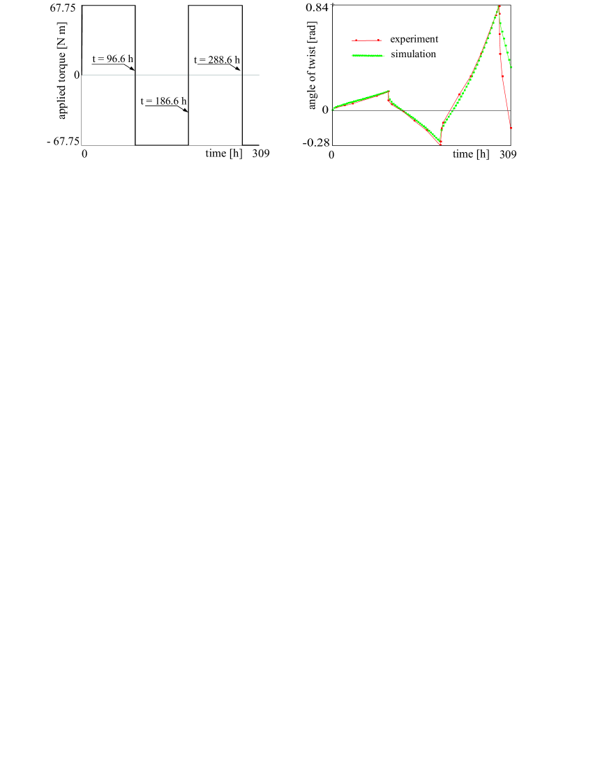
Figure 3. Applied torque as a stepwise function of time (left) and the twist angle as a function of time (right). The experimental data are taken from [12] and correspond to the constant temperature $T=250{}^{\text{o}}C$.

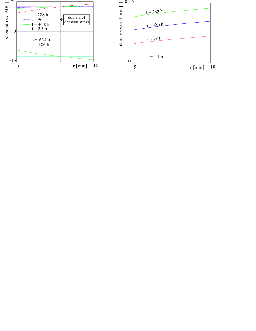
Figure 4. Distribution of the shear stress at different instances of time $t$ over the radius $r$ (left); distribution of the damage $\omega$ over the radius $r$ at different instances of time $t$ (right).

The dimensions of the thick-walled tubular specimen in the gage area are as follows: length $L=70$ mm, inner radius $r_{\text{i}}=5$ mm, outer radius $r_{\text{o}}=10$ mm. Here we use experimental creep data reported in [12]. The applied torque is a stepwise constant function of time shown in Fig. 3(left), the temperature is held constant during the entire process: $T=250{}^{\text{o}}C$. The experimentally measured twist is plotted against time on Fig. 3(right). The Norton creep law (13) is used in this section to simulate the torsion creep test; the relevant material parameters are summarized in Table 2.

As can be seen from Fig. 3(right), the transient phases of the non-stationary creep after load reversals can be captured by the model with a good accuracy. The overall effect of the creep damage is apparent; an increased creep strain rate is observed at the final part of the experiment. The effect of increasing amplitude of the (instant) elastic strain is captured by the model as well (cf. Fig. 3(right)). This effect is explained by the deterioration of elastic properties in the damaged material. Another important feature described by the model is that the transient stage is getting longer with progressive damage. Interestingly, this material phenomenon is explained by the current model as an interplay between the creep damage and the static recovery of the backstresses. The computed distribution of the shear stress (true stresses are used) at different instances of time is shown in Fig. 4(left). As is typical for creep problems, the stress distribution is becoming more uniform with time under constant applied stress. However, immediately after load reversals the stress distribution becomes inhomogeneous again.

Within the current simulation, the redistribution of stresses occur rather fast: within a few hours the stress distribution becomes nearly homogeneous (cf. the curve for $t=2.3$ h shown in Fig. 4(left)). Therefore, the pronounced transient effect observed in the simulation (cf. 3(right)) is due to the material behaviour, not due to the heterogeneous character of the stress distribution in the sample.

Examination of Fig. 4(left) shows another interesting feature: Within the sample there is a domain which is not affected by the redistribution of stresses. In this domain the absolute value of the shear stress is a constant function of time. Some authors refer to these stresses as “skeletal point stresses” or “referential stresses” [19]. The skeletal point stresses can be used for a rapid and simple interpretation of the experimental data.

The distribution of the damage variable $\omega$ is shown in 4(right). Here, $\omega$ is a smooth and monotonic function of the radius $r$. Although the stress distribution is nearly homogeneous, the material damage on the outer side is more pronounced than the damage on the inner side.

5. Discussion and conclusion

In the current work we put the main focus on the accurate simulation of the transient (non-stationary) creep response caused by abrupt load changes. A thermodynamically consistent finite-strain model with backstresses is proposed here; the nonlinear evolution of backstresses allows both for static and dynamic recovery. The model is coupled to the classical Kachanov-Rabotnov damage evolution such that the elastic properties deteriorate with damage.

The current framework allows one to consider the creep strain rate as an isotropic function of the effective stress. However, in order to reduce the huge manifold of possible constitutive assumptions, we use the equivalent stress $\sigma_{\text{eq}}$ as a creep potential. An important feature of the current definition of $\sigma_{\text{eq}}$ is that the maximum positive eigenvalue is replaced by its regularized (smoothed) counterpart $\sigma_{\text{reg max}}$. This regularization is needed for numerical reasons to ensure that the creep strain rate is a continuous function of the applied stress.

The strength-difference effect (also known as a tension-compression anisotropy) is taken into account by the evolution equation (39) since the corresponding equivalent stress $\sigma^{\lambda}_{\text{eq}}$ is sensitive to the sign of the uniaxial loading. Like any other model with backstresses, for its calibration one needs a series of experiments with varying stresses, e.g. tests with stress reversal. The applicability of the creep model is demonstrated using a FEM simulation of the non-monotonic torsion of a thick-walled tubular sample. Model predictions are compared to the experimental results obtained for the D16T aluminum alloy. A good correspondence between experimental and theoretical results can be achieved using the proposed model. The evolution of the stress distribution exhibits a “skeletal point” within the sample.

In the current study, only one backstress tensor is implemented. The generalization of the model to cover numerous backstresses is obvious (cf. [43, 51]). Further, we recall that the backstress tensor is purely deviatoric in this study. Generalization to backstresses with nonzero hydrostatic component is straightforward.

The main conclusion of the paper is that the practically important phenomenon of the non-stationary creep can be described using the nested multiplicative split of the deformation gradient. Additional multiplicative decompositions can be introduced to capture the damage-induced porosity [50] and the thermal expansion [29, 44] of the material. Moreover, the advocated here nested multiplicative split seems a reasonable tool for the construction of a unified model for creep-plasticity interaction.

The financial support provided by RFBR (grant number 16-08-00713 and 15-01-07631) is acknowledged.

Appendix A

The classical Euler-backward method (EBM) for the evolution equation (59) can be written in two equivalent forms:

$${}^{n+1}\mathbf{C}_{\text{cr}}={}^{n}\mathbf{C}_{\text{cr}}+\Delta t\ \mathbf{f}_{\text{cr}}({}^{n+1}\mathbf{C},{}^{n+1}\mathbf{C}_{\text{cr}},{}^{n+1}\mathbf{C}_{\text{ii}},{}^{n}\omega)\ {}^{n+1}\mathbf{C}_{\text{cr}},$$ (67)

$${}^{n+1}\mathbf{C}_{\text{cr}}=\big{[}\mathbf{1}-\Delta t\ \mathbf{f}_{\text{cr}}({}^{n+1}\mathbf{C},{}^{n+1}\mathbf{C}_{\text{cr}},{}^{n+1}\mathbf{C}_{\text{ii}},{}^{n}\omega)\big{]}^{-1}\ {}^{n}\mathbf{C}_{\text{cr}}.$$ (68)

Let us consider the following fixed-point iteration for the solution of (67)

$${}^{n+1}\mathbf{C}_{\text{cr}}^{(0)}:={}^{n}\mathbf{C}_{\text{cr}},\quad{}^{n+1}\mathbf{C}_{\text{cr}}^{(i+1)}={}^{n}\mathbf{C}_{\text{cr}}+\Delta t\ \mathbf{f}_{\text{cr}}({}^{n+1}\mathbf{C},{}^{n+1}\mathbf{C}_{\text{cr}}^{(i)},{}^{n+1}\mathbf{C}_{\text{ii}},{}^{n}\omega)\ {}^{n+1}\mathbf{C}_{\text{cr}}^{(i)},\ i=0,1,2,...$$ (69)

Since $\mathbf{f}_{\text{cr}}$ is a smooth function, the contractivity condition is satisfied for sufficiently small $\Delta t$. Therefore, the iterative process (69) converges to the exact solution of (67). To prove the symmetry of the solution ${}^{n+1}\mathbf{C}_{\text{cr}}$ pertaining to the classical EBM, it is sufficient to prove that ${}^{n+1}\mathbf{C}_{\text{cr}}^{(i)}\in Sym$ for all $i=1,2,3,...$. In other words, it suffice to prove that

$$\mathbf{f}_{\text{cr}}(\mathbf{C},\mathbf{C}_{\text{cr}},\mathbf{C}_{\text{ii}},\omega)\ \mathbf{C}_{\text{cr}}\in Sym\quad\text{for all}\quad\mathbf{C},\mathbf{C}_{\text{cr}},\mathbf{C}_{\text{ii}}\in Sym,\ \omega\in[0,1].$$ (70)

Recall that

$$\mathbf{f}_{\text{cr}}(\mathbf{C},\mathbf{C}_{\text{cr}},\mathbf{C}_{\text{ii}},\omega)\ \mathbf{C}_{\text{cr}}=2\ \lambda(\sigma^{\lambda}_{\text{eq}},\omega)\Big{(}\frac{\partial\sigma_{\text{eq}}}{\partial\tilde{\mathbf{\Sigma}}}\Big{)}^{\text{T}}\ \mathbf{C}_{\text{cr}}.$$ (71)

In order to prove (70), we introduce a fictitious deformation gradient and its parts as follows

$$\mathbf{F}=\mathbf{C}^{1/2},\ \mathbf{F}_{\text{cr}}=\mathbf{C}_{\text{cr}}^{1/2},\ \mathbf{F}_{\text{ii}}=\mathbf{C}_{\text{ii}}^{1/2}.$$ (72)

For these artificially introduced quantities, all the relations from Section 2.2 are valid. In particular, a symmetric tensor $\hat{\mathbf{\Sigma}}$ exists such that the right-hand side of (71) is obtained from the symmetric tensor $\lambda(\sigma^{\lambda}_{\text{eq}},\omega)\frac{\partial\sigma_{\text{eq}}}{\partial\hat{\mathbf{\Sigma}}}$ by the pull-back transformation $(\cdot)\mapsto\mathbf{F}^{\text{T}}_{\text{cr}}(\cdot)\mathbf{F}_{\text{cr}}$. Since the pull-back and its inverse preserve the symmetry, the symmetry condition (70) holds true.

An alternative (but more tedious) way of proving (70) is to note that $\mathbf{C}\tilde{\mathbf{T}}$ and $\mathbf{C}_{\text{cr}}\tilde{\mathbf{X}}$ are isotropic functions of $\mathbf{C}\mathbf{C}^{-1}_{\text{cr}}$ and $\mathbf{C}_{\text{cr}}\mathbf{C}^{-1}_{\text{ii}}$, respectively (cf. [45]), and $\Big{(}\frac{\partial\sigma_{\text{eq}}}{\partial\tilde{\mathbf{\Sigma}}}\Big{)}^{\text{T}}$ is an isotropic function of $\tilde{\mathbf{\Sigma}}=\mathbf{C}\tilde{\mathbf{T}}-\mathbf{C}_{\text{cr}}\tilde{\mathbf{X}}$.

Now let us prove that the modified Euler-backward method (60) preserves the symmetry as well. First we note that the modified method (60) yields the same solution as the classical method (68) whenever ${}^{n}\mathbf{C}_{\text{cr}}$ is properly scaled in (68):

$${}^{n+1}\mathbf{C}_{\text{cr}}=\overline{\big{[}\mathbf{1}-\Delta t\ \mathbf{f}_{\text{cr}}({}^{n+1}\mathbf{C},{}^{n+1}\mathbf{C}_{\text{cr}},{}^{n+1}\mathbf{C}_{\text{ii}},{}^{n}\omega)\big{]}^{-1}}\ {}^{n}\mathbf{C}_{\text{cr}}\quad\Rightarrow\\ \quad\text{there is}\ \beta>0\ \text{such that}\quad{}^{n+1}\mathbf{C}_{\text{cr}}=\big{[}\mathbf{1}-\Delta t\ \mathbf{f}_{\text{cr}}({}^{n+1}\mathbf{C},{}^{n+1}\mathbf{C}_{\text{cr}},{}^{n+1}\mathbf{C}_{\text{ii}},{}^{n}\omega)\big{]}^{-1}\ (\beta{}^{n}\mathbf{C}_{\text{cr}}).$$ (73)

In other words, the modified EBM (60) is the classical EBM (68) where the input quantity ${}^{n}\mathbf{C}_{\text{cr}}$ is scaled to enforce the incompressibility relation $\det({}^{n+1}\mathbf{C}_{\text{cr}})=1$. Since the classical EBM (68) preserves the symmetry, so does its modification (60).

References

- [1] H. Altenbach, J. Altenbach, and A. Zolochevsky, Erweiterte Deformationsmodelle und Versagenskriterien der Werkstoffmechanik. (Deutscher Verlag für Grundstoffindustrie, Stuttgart, 1995).
- [2] H. Altenbach, O. Morachkovsky, K. Naumenko, and A. Sychov, Geometrically nonlinear bending of thin-walled shells and plates under creep-damage conditions, Archive of Applied Mechanics 67, 339–352 (1997).
- [3] H. Altenbach and K. Naumenko, Modeling of Creep for Structural Analysis (Foundations of Engineering Mechanics (2007).
- [4] R. W. Bailey, The utilization of creep test data in engineering design, Proc. Inst. Mech. Eng. 131 (1935).
- [5] J.M. Borwein and J.D. Vanderwerff, Convex Functions. Constructions, Characterizations and Counterexamples. Encyclopedia of Mathematics and Its Applications 109 (Cabridge University Press, 2010).
- [6] J.T. Boyle and J. Spence. Stress analysis for creep (Butterworth-Heinemann, London, 1983).
- [7] C. Bröcker and A. Matzenmiller, An enhanced concept of rheological models to represent nonlinear thermoviscoplasticity and its energy storage behavior, Continuum Mechanics and Thermodynamics 25(6), 749–778 (2013).
- [8] E.W. Billington, Introduction to the Mechanics and Physics of Solids (Hilger, Bristol, 1986).
- [9] J.L. Chaboche, Constitutive equations for cyclic plasticity and cyclic viscoplasticity, International Journal of Plasticity 5, 247–302 (1989).
- [10] J. M. Corum, W.L. Greenstreet, K.C. Liu, C.E. Pugh, and R.W. Swindeman, Interim Guidelines for Detailed Inelastic Analysis of High-temperature Reactor System Components (ORNL-5014, Oak Ridge National Laboratory, 1974).
- [11] H. Garmestani, M.R. Vaghar, and E.W. Hart, A unified model for inelastic deformation of polycristalline materials - application to transient behavior in cyclic loading and relaxation, International Journal of Plasticity, 17 1367–1391 (2001).
- [12] B.V. Gorev, On the estimation of creep and long-term strength of structural elements using the method of characteristic parameters. Message 1., Problems of Strength 4, 30–36 (1979).
- [13] M.O. Faruque, On the description of cyclic creep and rate dependent plastic deformation, Acta Mechanika 55, 123–136 (1985)
- [14] M.O. Faruque, M. Zaman, and M.I. Hossain, Creep constitutive modeling of an aluminum alloy under multiaxial and cyclic loading, International Journal of Plasticity 12(6), 761–780 (1996).
- [15] X. Feaugas, On the origin of the tensile flow stress in the stainless steel AISI 316L at 300 K: back stress and effective stress, Acta Materialia, 47(13) 3617–3632 (1999).
- [16] W.N. Findley, U.W. Cho, and J.L. Ding, Creep of metals and plastic under combined stresses, a review, Trans. ASME. J. Eng. Mater. Technol. 101, 365–368 (1979).
- [17] Y. Gorash, H. Altenbach, and G. Lvov, Modelling of high-temperature inelastic behaviour of the austenitic steel AISI type 316 using a continuum damage mechanics approach, The Journal of Strain Analysis for Engineering Design 47(4), 229–243 (2012).
- [18] S. Hartmann and P. Neff, Polyconvexity of generalized polynomial-type hyperelastic strain energy functions for near-incompressibility, International Journal of Solids and Structures 40, 2767–2791 (2003).
- [19] B.D. Hayhurst and F.A. Leckie, The effect of creep constitutive and damage relationships upon the rupture time of a solid circular torsion bar, J. Mech. Phys. Solids 21, 431–446 (1973).
- [20] D. Helm, Formgedächtnislegierungen, experimentelle Untersuchung, phänomenologische Modellierung und numerische Simulation der thermomechanischen Materialeigenschaften (Phd-thesis, Universitätsbibliothek Kassel, 2001).
- [21] L.M. Kachanov, Time of the rupture process under creep conditions (Russian), Izv. AN SSSR. Otd. Tekh. Nauk 8, 26–31 (1958).
- [22] M. Kawai, Creep hardening rule under multiaxial repeated stress changes, JSME Int. J. 38A, 201–212 (1995).
- [23] R. Kießling, R. Landgraf, R. Scherzer, and J. Ihlemann, Introducing the concept of directly connected rheological elements by reviewing rheological models at large strains, International Journal of Solids and Structures, 97 98, 650–667 (2016).
- [24] J. M. Klebanov, Constitutive equations for creep under changing multiaxial stresses, European Journal of Mechanics - A/Solids 18(3), 433–442 (1999).
- [25] Y. Kostenko, H. Almstedt, K. Naumenko, S. Linn, and A. Scholz, Robust methods for creep fatigue analysis of power plant components under cyclic transient thermal loading. In: ASME turbo Expo 2013: turbine technical conference and exposition, American Society of Mechanical Engineers, 8 pages (2013).
- [26] A. Krawietz, Materialtheorie. Mathematische Beschreibung des phänomenologischen thermomechanischen Verhalten (Springer, Berlin, 1986).
- [27] R.D. Krieg, J.C. Swerengen, and W.B. Jones, A Physically Based Internal Variable Model for Rate Dependent Plasticity, 245–271, in Unified Constitutive Equations for Creep and Plasticity, editor A.K. Miller (Elsevier, 1987).
- [28] J. Lemaitre and J.-L. Chaboche. Mechanics of Solid Materials. (Cambridge University Press, Cambridge, 1990).
- [29] A. Lion, Constitutive modelling in finite thermoviscoplasticity: a physical approach based on nonlinear rheological elements, International Journal of Plasticity 16, 469–494 (2000).
- [30] N.N. Malinin and G.M. Khadjinsky, Theory of creep with anisotropic hardening, Int. J. Mech. Sci. 14, 235–246 (1972).
- [31] S.T. Mileiko and Yu.N. Rabotnov, Some results of an experimental study of short-time creep in uniaxial tension, Journal of Applied Mechanics and Technical Physics 7(5), 107–113 (1966).
- [32] S. Murakami and N. Ohno, Constitutive equations of creep based on the concept of a creep hardening surface, Int. J. Solids Struct. 18, 597–609 (1982).
- [33] Z. Mroz and W.A. Trampczynski, On the creep-hardening rule for metals with a memory of maximal prestress, International Journal of Solids and Structures 20(5), 467–468 (1984).
- [34] K. Naumenko, H. Altenbach, and A. Kutschke, A combined model for hardening, softening, and damage processes in advanced heat resistant steels at elevated temperature, International Journal of Damage Mechanics 20, 578–597 (2010).
- [35] K. Naumenko, A. Kutschke, Y. Kostenko, and T. Rudolf, Multi-axial thermo-mechanical analysis of power plant components from 9 12%Cr steels at high temperature, Eng Fract Mech 78, 1657–1668 (2011).
- [36] Y. Ohashi, N. Ohno, and M. Kawai, Evaluation of creep constitutive equations for type 304 stainless steel under repeated multiaxial loading, Journal of Engineering Materials and Technology 104(3), 159–164 (1982).
- [37] N. Ohno, S. Murakami, and T. Ueno, A constitutive model of creep describing creep recovery and material softening caused by stress reversals, Journal of Engineering Materials and Technology 107(1), 1–6 (1985).
- [38] N. Ohno, Recent topics in constitutive modelling of cyclic plasticity and viscoplasticity, Appl. Mech. Rev. 43, 283–295 (1990).
- [39] V. Palmov, Vibrations in Elasto-Plastic Bodies (Springer, Berlin, 1998).
- [40] W. Prager, Der Einfluß der Verformung auf die Fließbedingung zähplastischer Körper, ZAMM 15(1/2), 76–80 (1935).
- [41] Yu. N. Rabotnov, Creep Problems in Structural Members (North-Holland, Amsterdam, 1969).
- [42] A. Scholz and C. Berger, Deformation and life assessment of high temperature materials under creep fatigue loading, Materialwissenschaft und Werkstofftechnik. 36(11), 722–730 (2005).
- [43] A. V. Shutov, C. Kuprin, J. Ihlemann, M.F.-X. Wagner, and C. Silbermann, Experimentelle Untersuchung und numerische Simulation des inkrementellen Umformverhaltens von Stahl 42CrMo4, Materialwissenschaft und Werkstofftechnik, 41(9) (2010) 765–775.
- [44] A.V. Shutov and J. Ihlemann, On the simulation of plastic forming under consideration of thermal effects, Materials Science & Engineering Technology 42(7), 632–638 (2011).
- [45] A.V. Shutov and R. Kreißig, Finite strain viscoplasticity with nonlinear kinematic hardening: Phenomenological modeling and time integration, Computer Methods in Applied Mechanics and Engineering 197, 2015–2029 (2008).
- [46] A.V. Shutov and R. Kreißig, Geometric integrators for multiplicative viscoplasticity: Analysis of error accumulation, Computer Methods in Applied Mechanics and Engineering 199, 700–711 (2010).
- [47] A.V. Shutov, R. Landgraf, and J. Ihlemann, An explicit solution for implicit time stepping in multiplicative finite strain viscoelasticity, Computer Methods in Applied Mechanics and Engineering 265, 213–225 (2013).
- [48] A.V. Shutov, S. Pfeiffer, and J. Ihlemann, On the simulation of multi-stage forming processes: invariance under change of the reference configuration, Materials Science and Engineering Technology 43(7), 617–625 (2012).
- [49] A.V. Shutov and J. Ihlemann, Analysis of some basic approaches to finite strain elasto-plasticity in view of reference change, International Journal of Plasticity 63, 183–197 (2014).
- [50] A.V. Shutov, C. B. Silbermann, and J. Ihlemann, Ductile damage model for metal forming simulations including refined description of void nucleation, International Journal of Plasticity 71, 195–217 (2015).
- [51] A. V. Shutov, Efficient implicit integration for finite-strain viscoplasticity with a nested multiplicative split. Computer Methods in Applied Mechanics and Engineering 306(1), 151–174 (2016).
- [52] D. Slavik and H. Sehitoglu, A unified creep-plasticity model suitable for thermo-mechanical loading, NASA CP 10010, 295–306 (1988).
- [53] O.V. Sosnin, Creep in materials with different tension and compression behaviour, Journal of Applied Mechanics and Technical Physics 115, 832–835 (1970).
- [54] S. Straub, Verformungsverhalten und Mikrostruktur warmfester martensitischer 12%-Chromstähle (Dissertation, Universität Erlangen-Nürnberg, Fortschr.-Ber. VDI Reihe 5, Nr. 405, Düsseldorf.
- [55] M. A. Zapara, N. D. Tutyshkin, W. H. Müller, and R. Wille, Experimental study and modeling of damage of Al alloys using tensor theory, Continuum Mech. Thermodyn. 22, 99–120 (2010).
- [56] M. Zapara, N. Tutyshkin, W.H. Müller, and R. Wille, Constitutive equations of a tensorial model for ductile damage of metals, Continuum Mech. Thermodyn. 24, 697–717 (2012).
- [57] A. Zolochevsky, S. Sklepus, Yu. Kozmin, A. Kozmin, D. Zolochevsky, and J. Betten, Constitutive equations of creep under changing multiaxial stresses for materials with different behavior in tension and compression, Forschung im Ingenieurwesen 68, 182–196 (2004).
- [58] A. Zolochevsky and G. Z. Voyiadjis, Theory of creep deformation with kinematic hardening for materials with different properties in tension and compression, International Journal of Plasticity 21, 435–462 (2005).
- [59] V. Velay, G. Bernhart, and L. Penazzi, Cyclic behavior modeling of a tempered martensitic hot work tool steel, International Journal of Plasticity 22, 459–496 (2006).
- [60] I. Vladimirov, M. Pietryga, and S. Reese, On the modelling of non-linear kinematic hardening at finite strains with application to springback – Comparison of time integration algorithms, Int. J. Numer. Meth. Engng 75, 1–28 (2008).