Perspective: Dissipative Particle Dynamics

Abstract

Dissipative particle dynamics (DPD) belongs to a class of models and computational algorithms developed to address mesoscale problems in complex fluids and soft matter in general. It is based on the notion of particles that represent coarse-grained portions of the system under study and allow, therefore, to reach time and length scales that would be otherwise unreachable from microscopic simulations. The method has been conceptually refined since its introduction almost twenty five years ago. This perspective surveys the major conceptual improvements in the original DPD model, along with its microscopic foundation, and discusses outstanding challenges in the field. We summarize some recent advances and suggests avenues for future developments.

I Introduction

The behaviour of complex fluids and soft matter in general is characterized by the presence of a large range of different time and space scales. Any attempt to resolve simultaneously several time scales in a single simulation scheme is confronted by the problem of taking a prohibitively large number of sufficiently small time steps. Typically one proceeds hierarchically Berendsen (2007), by devising models and algorithms appropriate to the length and time scales one is interested in. Leaving aside quantum effects negligible for soft matter, at the bottom of the hierarchy we have Hamilton’s equations, with accurate albeit approximate potential energy functions, which are solved numerically with molecular dynamics (MD). Nowadays some research teams can simulate billions of particles for hundreds of nanoseconds Heinecke et al. (2015). This opens up the possibility to study very detailed, highly realistic molecular models that capture essentially all the microscopic details of the system. This is, of course, not enough in many situations encountered in soft matter and life sciences Shillcock (2008). One can always think of a problem well beyond computational capabilities: from the folding of large proteins, to the replication of DNA, or the simulation of an eukariotic cell, or the simulation of a mammal, including its brain. While we are still very far from even well-posing some of these problems, it is obvious that science is pushing strongly towards more and more complex systems.

Instead of using atoms moving with Hamilton’s equations to describe matter, one can take a continuum approach in which fields take the role of the basic variables. Navier-Stokes-Fourier hydrodynamics, or elasticity, or many of the different continuum theories for complex fluid systems are examples of this approach Öttinger (2005). These continuum theories are, in fact, coarse-grained versions of the atomic system that rely on two key related concepts: 1) the continuum limit—i. e. a “point” of space on which the field is defined is, in fact, a volume element containing a large number of atoms Batchelor (1967), and 2) the local equilibrium assumption—i. e. these volumes are large enough to reproduce the thermodynamic behaviour of the whole system de Groot and Mazur (1964). The quantities from one volume element to its neighbour are assumed to change little and this allows the powerful machinery of partial differential equations to describe mathematically the system at the largest scales, allowing even to find analytical solutions for many situations. Nevertheless, the continuum equations are usually non-linear and analytical solutions are not always possible. One resorts then to numerical methods to solve the equations. Computational fluid dynamics (CFD) has evolved into a sophisticated field in numerical analysis with a solid mathematical foundation.

The length scales that can be addressed by continuum theories range from microns to parsecs. Remarkably, the same equations (with the same thermodynamics and transport coefficients) can be used at very different scales. Many of the interesting phenomena that occur in complex fluids occur at the mesoscale. The mesoscale can be roughly defined as the spatio-temporal scales ranging from 10–$10^{4}$ nm and 1–$10^{6}$ ns. These scales require a number of atoms that make the simulation with MD readily unfeasible. On the other hand, it was shown in the early days of computer simulations by Alder and Wainwright Alder and Wainwright (1970) that hydrodynamics is valid at surprisingly small scales. Therefore, there is a chance to use continuum theory down to the mesoscale. However, at these short length scales the molecular discreteness of the fluid starts to manifest itself. For example, a colloidal particle of submicron size experiences Brownian motion which is negligible for macroscopic bodies like submarine ships. In order to address these small scales one needs to equip field theories like hydrodynamics with fluctuating terms, as pioneered by Landau and Lifshitz Landau and Lifshitz (1959). The resulting equations of fluctuating hydrodynamics also receive the name of Landau-Lifshitz-Navier-Stokes (LLNS) equation. There is much effort in the physics/mathematical communities to formulate numerical algorithms with the standards of usual CFD for the solution of stochastic partial differential equations modeling complex fluids at mesoscales Naji et al. (2009); Uma et al. (2011); Shang et al. (2012); Donev et al. (2010); Oliver et al. (2013); Donev and Vanden-Eijnden (2014); Donev et al. (2014); Plunkett et al. (2014); De Corato et al. (2016).

While the use of fluctuating hydrodynamics may be appropriate at the mesoscale, there are many systems for which a continuum hydrodynamic description is not applicable (or it is simply unknown). Proteins, membranes, assembled objects, polymer systems et c. may require unaccessible computational resources to be addressed with full microscopic detail but a continuum theory may not exist. In these mesoscale situations, the strategy to retain some chemical specificity is to use coarse-grained descriptions in which groups of atoms are treated as a unit Voth (2009). While the details of how to do this are very system specific, and an area of intense active research (see reviews in Refs. Noid (2013); Brini et al. (2013); Lopez et al. (2014)), it is good to know that there is a well defined and sounded procedure for the construction of coarse-grained descriptions Green (1952); Zwanzig (1961) that is known under the names of non-equilibrium statistical mechanics, Mori-Zwanzig theory, or the theory of coarse-graining Grabert (1982); Zubarev D. (1996); Español (2004); Öttinger (2005). Simulating everything, everywhere, with molecular detail can be not only very expensive but also unnecessary. In particular, water is very expensive to simulate and sometimes its effect is just to propagate hydrodynamics. Hence there is an impetus to develop at least coarse-grained solvent models, but retain enough solute molecular detail to render chemical specificity.

At the end of the 20th century the simulation of the mesoscale was attacked from a computational point of view with a physicist intuitive, quick and dirty, approach. Dissipative particle dynamics (DPD) was one of the products, among others Malevanets and Kapral (1999); Succi (2001); Holm and Kremer (2009); Dünweg and Ladd (2009); Gompper et al. (2009); Donev et al. (2009), of this approach. DPD is a point particle minimal model constructed to address the simulation of fluid and complex systems at the mesoscale, when hydrodynamics and thermal fluctuations play a role. The popularity of the model stems from its algorithmic simplicity and its enormous versatility. Just by varying at will the conservative forces between the dissipative particles one can readily model complex fluids like polymers, colloids, amphiphiles and surfactants, membranes, vesicles, phase separating fluids, et c. Due to its simple formulation in terms of symmetry principles (Galilean, translational, and rotational invariances) it is a very useful tool to explore generic or universal features (scaling laws, for example) of systems that do not depend on molecular specificity but only on these general principles. However, detailed information highly relevant for industrial and technological processes requires the inclusion of chemical detail in order to go beyond qualitative descriptions.

DPD, as originally formulated, does not include this chemical specificity. This is not a drawback of DPD per se, as the model is regarded as a coarse-grained version of the system. Any coarse-graining process eliminates details from the description and keeps only the relevant ones associated to the length and time scales of the level of description under scrutiny. However, as it will be apparent, the original DPD model could be regarded as being too simplistic and one can formulate models that capture more accurate information of the system with comparable computational efficiency.

Since its initial introduction, the question “What do the dissipative particles represent?” has lingered in the literature, with intuitively appealing but certainly vague answers like “groups of atoms moving coherently”. In the present Perspective we aim at answering this question by reviewing the efforts that have been taken in this direction. We offer a necessarily brief overview of applications, and discuss some open questions and unsolved problems, both of fundamental and applied nature. Since the initial formulation of the DPD model a number of excellent reviews Warren (1998); Español (2004); Pivkin et al. (2010); Moeendarbary et al. (2010); Guigas et al. (2011); Lu and Wang (2013); Ghoufi et al. (2013); Liu et al. (2014), and dedicated workshops Brennan and Lísal (2009); Mousseau and Montréal (2014), have kept the pace of the developments. We hope that the present perspective complements these reviews with a balanced view about the more recent advances in the field. We also provide a route map through the different DPD variant models and their underlying motivation. In this doing, we hope to highlight a unifying conceptual view for the DPD model and its connection with the microscopic and continuum levels of description.

This Perspective is organized as follows. In Sec. II we consider the original DPD model with its virtues and limitations. In Sec. III we review models that have been formulated in order to avoid the limitations of the original DPD model. The SDPD model, which is the culmination of the previous models that links directly to the macroscopic level of description (Navier-Stokes) is considered in Sec. IV. The microscopic foundation of the DPD model is presented in Sec. V. Finally, we present some selected applications in Sec. VI and conclude in Sec. VII.

II The original DPD model

The original DPD model was introduced by Hoogerbrugge and Koelman Hoogerbrugge and Koelman (1992), and was formulated by the present authors as a proper statistical mechanics model shortly after Español and Warren (1995). The DPD model consists on a set of point particles that move off-lattice interacting with each other with three types of forces: a conservative force deriving from a potential, a dissipative force that tries to reduce radial velocity differences between the particles, and a further stochastic force directed along the line joining the center of the particles. The last two forces can be termed as a “pair-wise Brownian dashpot” which, as opposed to ordinary Langevin or Brownian dynamics, is momentum conserving. The Brownian dashpot is a minimal model for representing viscous forces and thermal noise between the “groups of atoms” represented by the dissipative particles. Because of momentum conservation the behaviour of the system is hydrodynamic at sufficiently large scales Español (1995); Marsh et al. (1997); Boromand et al. (2015).

Figure 1: Dissipative particles interact pair-wise with a conservative linear repulsive force, and a Brownian dashpot made of a friction force that reduces the relative velocity between the particles and a stochastic force that gives kicks of equal size and opposite directions to the particles. These forces vanishes beyond a cutoff radius $r_{c}$.

The stochastic differential equations of motion for the dissipative particles are Español and Warren (1995)

$$\dot{\bf r}_{i}= {\bf v}_{i}$$

$$m_{i}\dot{\bf v}_{i}= -\frac{\partial V}{\partial{\bf r}_{i}}-\sum_{j}\gamma\omega^{D}(r_{ij})({\bf v}_{ij}\cdot{\bf e}_{ij}){\bf e}_{ij}$$

$$+\sum_{j}\sigma\omega^{R}(r_{ij})\frac{dW_{ij}}{dt}{\bf e}_{ij}$$ (1)

where $r_{ij}=|{\bf r}_{i}-{\bf r}_{j}|$ is the distance between particles $i,j$, ${\bf v}_{ij}={\bf v}_{i}-{\bf v}_{j}$ is the relative velocity and ${\bf e}_{ij}={\bf r}_{ij}/r_{ij}$ is the unit vector joining particles $i$ and $j$. $dW_{ij}$ is an independent increment of the Wiener process. In Eq. (1), $\gamma$ is a friction coefficient and $\omega^{D}(r_{ij}),\omega^{R}(r_{ij})$ are bell-shaped functions with a finite support that render the dissipative interactions local. Validity of the fluctuation-dissipation theorem requires Español and Warren (1995) $\sigma$ and $\gamma$ to be linked by the relation $\sigma^{2}=2\gamma k_{\mathrm{B}}T$ and also $\omega^{D}(r_{ij})=[\omega^{R}(r_{ij})]^{2}$. Here $k_{\mathrm{B}}$ is Boltzmann’s constant and $T$ is the system temperature. As a result, the stationary probability distribution of the DPD model is given by the Gibbs canonical ensemble

$$\rho(\{{\bf r},{\bf v}\}) =\frac{1}{Z}\exp\left\{-\beta\sum_{i}^{N}m_{i}\frac{{\bf v}_{i}^{2}}{2}-\beta V(\{{\bf r}\})\right\}$$ (2)

The potential energy $V(\{{\bf r}\})$ is a suitable function of the positions of the dissipative particles that is translationally and rotationally invariant in order to ensure linear and angular momentum conservation. In the original formulation the form of the potential function was taken of the simplest possible form

$$V(\{{\bf r}\}) =\frac{1}{2}\sum_{ij}a_{ij}(1-r_{ij}/r_{c})^{2}$$ (3)

where $a_{ij}$ is a particle interaction constant and $r_{c}$ is a cutoff radius. This potential produces a linear force with the form of a Mexican hat function of finite range. Without any other guidance, the weight function $\omega^{R}(r)$ in the dissipative and random forces is given by the same linear functional form. Complex fluids can be modeled through mesostructures constructed by adding additional interactions (springs and/or attractive or repulsive potentials between certain particles) to the particles. Groot and Warren Groot and Warren (1997) offered a practical route to select the parameters in a DPD simulation by matching compressibility and solubility parameters of the model to real systems.

The soft nature of the weight functions in DPD allows for large time steps, as compared with MD that needs to deal with steep repulsive potentials. However too large time steps lead to numerical errors that depend strongly on the numerical algorithm used. The area of numerical integrators for the stochastic differential equations of DPD has received attention during the years with increasingly sophisticated methods. Starting from the velocity Verlet implementation of Ref. Groot and Warren (1997) and the self-consistent reversible scheme of Pagonabarraga and Hagen Pagonabarraga and Hagen (1998), the field has evolved towards splitting schemes Shardlow (2003); Nikunen et al. (2003); Defabritiis et al. (2006); Serrano et al. (2006); Thalmann and Farago (2007); Chaudhri and Lukes (2010). A Shardlow Shardlow (2003) scheme has been recommended after comparison between different integrators Nikunen et al. (2003), but there are also other recent more efficient proposals Litvinov et al. (2010); Leimkuhler and Shang (2015); Farago and Grønbech-Jensen (2016).

Because of momentum conservation, the original DPD model in Eqs. (1)–(3) can be regarded as a (toy) model for the simulation of fluctuating hydrodynamics of a simple fluid. As a model for a Newtonian fluid at mesoscales the DPD model has been used for the simulation of hydrodynamics flows in several situations Jury et al. (1999a); Keaveny et al. (2005); Chen et al. (2006a); van de Meent et al. (2008); Tiwari et al. (2008); Steiner et al. (2009); Filipovic et al. (2011). It should be obvious, though, that the fact that DPD conserves momentum does not makes it the preferred method for solving hydrodynamics. MD is also momentum conserving and can be used to solve hydrodynamics; for a recent review see Kadau et al. Kadau et al. (2010). However, in terms of computational efficiency hydrodynamic problems are best addressed with CFD methods with, perhaps, inclusion of thermal fluctuations.

In addition, the original DPD model suffers from several limitations that downgrade its utility as a LLNS solver. The first one is the thermodynamic behaviour of the model. Taken as a particle method, the DPD model has an equation of state that is fixed by the conservative interactions. The linear conservative forces of the original DPD model produce an unrealistic equation of state that is quadratic in the density Groot and Warren (1997). The quadratic equation of state in DPD seems to be a general property of soft sphere fluids at high overlap density. A well-known exemplar is the Gaussian core model Louis et al. (2000). These systems have been termed mean-field fluids and this includes the linear DPD potential in Eq. (3). Many thermodynamic properties for the linear DPD potential can be obtained by using standard liquid state theory and it has been our experience that the HNC integral equation closure works exceptionally well in describing the behaviour of DPD in the density regime of interest Warren et al. (2013); Warren and Vlasov (2014); Fraaije et al. (2016). Note that while it is possible to fit the compressibility (related to second derivatives of the free energy) to that of water, for example, the pressure (related to first derivatives) turns out to be unrealistic. The conservative forces of the original model are not flexible enough to specify the thermodynamic behaviour as an input of the simulation code Trofimov et al. (2002).

A second limitation is due to too simplistic friction forces. The central friction force in Eq. (1) implies that when a dissipative particle passes a second, reference particle, it will not exert any force on the reference particle unless there is a radial component to the velocity Español (1997a, 1998). Nevertheless, on simple physical grounds one would expect that the passing dissipative particle would drag in some way the reference particle due to shear forces. Of course, if many DPD particles are involved simultaneously in between the two particles, this will result in an effective drag. The same is true for a purely conservative molecular dynamics simulation. It would be nice, though, to have this effect captured directly in terms of modified friction forces in a way that a smaller number of particles need to be used to reproduce large scale hydrodynamics. Note that the viscosity of the DPD model cannot be specified beforehand, and only after a recourse to the methods of kinetic theory can one estimate the friction coefficient to be imposed in order to obtain a given viscosity Español (1995); Marsh et al. (1997); Masters and Warren (1999); Evans (1999). As we will see, inclusion of more sophisticated shear forces allows for a more direct connection with Navier-Stokes hydrodynamics.

A third limitation of DPD as a mesoscale hydrodynamic solver is the fact that the DPD model (in an identical manner as MD) is hardwired to the scale. What we mean with this is that given a physical problem, with a characteristic length scale, we may always put a given number of dissipative particles and parametrize the model in order to recover some macroscopic information (typically, compressibilities and viscosity). However, if one uses a different number of particles for exactly the same physical situation, one should start over and reparametrize the system again. This is certainly very different from what one would expect from a Navier-Stokes solver, that specifies the equation of state and viscosity irrespective of the scale, and one simply worries about having a sufficiently large number of points to resolve the characteristic length scales of the flow. In other words, in DPD there is no notion of resolution, grid refinement, and convergence as in CFD. There have been attempts to restore a scale free property for DPD Español (1998); Füchslin et al. (2009); Arienti et al. (2011), even for bonded interactions Spaeth et al. (2010). To get this property, the parameters in the model need to depend on the level of coarse-graining, but this is not specified in the original model. Closely related to this lack of scaling is the fact that there is no mechanism in the model to switch off thermal fluctuations depending on the scale at which the model is operating. On general statistical mechanics grounds, thermal fluctuations should scale as $1/\sqrt{N}$ where $N$ is the number of degrees of freedom coarse-grained into one coarse-grained (CG) particle. As the dissipative particles represent larger and larger volume elements, they should display smaller and smaller fluctuations. But there is no explicit volume or size associated to a dissipative particle. This problem is crucial, for instance, in the case of suspended colloidal particles or in microfluidics applications where flow conditions and the physical dimensions of the suspended objects or physical dimensions of the operating device determine whether and, more importantly, to what extent thermal fluctuations come into play.

Finally, another limitation of the DPD model is that it cannot sustain temperature gradients. Energy in the system is dissipated and not conserved, and the Brownian dashpot forces of DPD act as a thermostat.

III MDPD, EDPD, FPM

During the years, the DPD model has been enriched in several directions in order to deal with all the above limitations. In this Section we briefly review these enriched DPD models.

The many-body (or multi-body) dissipative particle dynamics (MDPD) method stands for a modification of the original DPD model in which the purely repulsive conservative forces of the classic DPD model are replaced by forces deriving from a many-body potential; thus the scheme is still covered by Eqs. (1)–(2), but a many-body $V(\{{\mathbf{r}}\})$ is substituted for Eq. (3). The MDPD method was originally introduced by Pagonabarraga and Frenkel Pagonabarraga and Frenkel (2001), Warren Warren (2001), and independently by Groot, foo (a) and subsequently modified and improved by Trofimov et al. Trofimov et al. (2002), reaching a level of maturity Warren (2003a); Merabia and Pagonabarraga (2007); Ghoufi and Malfreyt (2010); Arienti et al. (2011); Ghoufi et al. (2013); Warren (2013); Atashafrooz and Mehdipour (2016). The key innovation of the MDPD is the introduction of a density variable $d_{i}=\sum_{j\neq i}W(r_{ij})$, as well as a free energy $\psi(d_{i})$ associated to each dissipative particle. Here $W(r)$ is a normalized bell-shaped weight function that ensures that the density $d_{i}$ is high if many particles are accumulated near the $i$-th particle. The potential of interaction of these particles is assumed to be of the form $V=\sum_{i}\psi(d_{i})$ Warren (2003b). This is a many-body potential of a form similar to the embedded atom potential in MD simulations Daw and Baskes (1984); Daw et al. (1993). For multi-component mixtures the many-body potential may be generalized to depend on partial local densities.

Despite its many-body character, the resulting forces are still pair-wise, and implementation is straightforward. However, not all pair-wise force laws correspond to a many-body potential. Indeed the existence of such severely constrains the nature of the force laws, and some errors have propagated into the literature (see discussion in Ref. Warren (2013)). In Appendix A we explore how the force law is constrained by the weight function $W(r)$. The message is: if in doubt, always work from $V(\{{\mathbf{r}}\})$.

MDPD escapes the straitjacket of mean-field fluid behaviour by modulating the thermodynamic behaviour of the system directly at the interaction level between the particles. This allows for more general equations of state than in the original DPD model, which is a special case where the one-body terms are linear in local densities. Indeed, one can easily engineer a van der Waals loop in the equation of state to accommodates vapor-liquid coexistence. But this in itself is not enough to stabilize a vapour-liquid interface, since one should additionally ensure that the cohesive contribution is longer-ranged than the repulsive contribution. This can be achieved for example by using different ranges for the attractive and repulsive forces Warren (2001, 2003a), or modelling the square gradient term in the free energy Tiwari and Abraham (2006).

The energy-conserving dissipative particle dynamics model (EDPD) was introduced simultaneously and independently by Bonet Avalós and Español Bonet Avalos and Mackie (1997); Español (1997b) as a way to extend the DPD model to non-isothermal situation. In this case, the key ingredient is an additional internal energy variable associated to the particles. The behaviour of the model was subsequently studied Bonet Avalos and Mackie (1999); Ripoll et al. (1998); Ripoll and Español (2000); Ripoll and Ernst (2004). The method has been compared with standard flow simulations Abu-Nada (2011); Yamada et al. (2011), and recently a number of interesting applications have emerged Chaudhri and Lukes (2009); Lísal et al. (2011), including heat transfer in nanocomposites Qiao and He (2007), shock detonations Maillet et al. (2011), phase change materials for energy storage Rao et al. (2012), shock loading of a phospholipid bilayer Ganzenmüller et al. (2012), chemically reacting exothermic fluids Brennan et al. (2014, 2016), thermoresponsive polymers Li et al. (2015a), and water solidification Johansson et al. (2016).

The fluid particle model (FPM) was devised as a way to overcome the limitation of the simplistic friction forces in DPD Español (1997a, 1998). The method introduced, in addition to radial friction forces, shear forces that depend not only on the approaching velocity but also on the velocity differences directly. Shear forces have been reconsidered recently Junghans et al. (2008). The resulting forces are non-central and do not conserve angular momentum. In order to restore angular momentum conservation a spin variable is introduced. Heuristically, the spin variable is understood as the angular momentum relative to the center of mass of the fluid particle. The model has been used successfully by Pryamitsyn and Ganesan Pryamitsyn and Ganesan (2005) in the simulation of colloidal suspensions, where each colloid is represented by just one larger dissipative particle, an approach also used by Pan et al. Pan et al. (2008).

IV DPD from top-down: The SDPD model

While MDPD is still isothermal and EDPD still uses conservative forces too limited to reproduce arbitrary thermodynamics, the two enrichments of a density variable and an internal energy variable introduced by these models suggest a view of the dissipative particles as truly thermodynamic subsystems of the whole system, consistently with the local equilibrium assumption in continuum hydrodynamics. There have been a number of works trying to formalize this view of “moving fluid particles” in terms of Voronoi cells of points moving with the flow field Español et al. (1997). Flekkøy et al. formulated a (semi) bottom-up approach for constructing a model of fluid particles with the Voronoi tessellation Flekkøy and Coveney (1999); Flekkøy et al. (2000). A thermodynamically consistent Lagrangian finite volume discretization of LLNS using the Voronoi tessellation was presented by Serrano and Español Serrano and Español (2001) and compared favourably Serrano et al. (2002) with the models in Refs. Flekkøy and Coveney (1999) and Flekkøy et al. (2000). While this top-down modeling based on the Voronoi tessellation is grounded in a solid theoretical framework, it has not found much application due, perhaps, to the computational complexity of a Lagrangian update of the Voronoi tessellation foo (b).

In an attempt to simplify the Lagrangian finite Voronoi volume discretization model, the smoothed dissipative particle dynamics (SDPD) model was introduced shortly after Español and Revenga (2003), based on its precursor Español et al. (1999). SDPD is a thermodynamically consistent particle model based on a particular version of smoothed particle hydrodynamics (SPH) that includes thermal fluctuations. SPH is a mesh-free Lagrangian discretization of the Navier-Stokes equations (NSE) differing from finite volumes, elements, or differences in that a simple smooth kernel is used for the discretization of space derivatives. This leads to a model of moving interacting point particles whose simulation is very similar to MD. SPH was introduced in an astrophysical context for the simulation of cosmic matter at large scales Lucy (1977); Gingold and Monaghan (1978), but has been applied since then to viscous and thermal flows Liu and Liu (2003, 2010), including multi-phasic flow Wang et al. (2016). An excellent recent critical review on SPH is given by Violeau and Rogers Violeau and Rogers (2016).

In the particular SPH discretization given by SDPD of the viscous terms in the NSE, the resulting forces have the same structure of the shear friction forces in the FPM. By casting the model within the universal thermodynamically consistent generic framework Öttinger (2005), thermal fluctuations are introduced consistently in SDPD by respecting an exact fluctuation-dissipation theorem at the discrete level. Therefore, SDPD (as opposed to SPH) can address the mesoscopic realm where thermal fluctuations are important.

The SDPD model consists on $N$ point particles characterized by their positions and velocities ${\bf r}_{i},{\bf v}_{i}$ and, in addition, a thermal variable like the entropy $S_{i}$ (by a simple change of variables, one can also use alternatively the internal energy $\epsilon_{i}$ or the temperature $T_{i}$). Each particle is understood as a thermodynamic system with a volume ${\cal V}_{i}$ given by the inverse of the density $d_{i}=\sum_{i}^{N}W(r_{ij})$, a fixed constant mass $m_{i}$, and an internal energy $\epsilon_{i}=E(S_{i},m_{i},{\cal V}_{i})$ which is a function of the entropy of the particle, its mass (i. e. number of moles), and volume. The functional form of $E(S,M,{\cal V})$ is assumed, through the local equilibrium assumption, to be the same function that gives the global thermodynamic behaviour of the fluid system (but see below). The equations of motion of the independent variables are Español and Revenga (2003)

$$d{\bf r}_{i}= {\bf v}_{i}dt$$

$$md{\bf v}_{i}= \sum_{j}\left[\frac{P_{i}}{d_{i}^{2}}+\frac{P_{j}}{d_{j}^{2}}\right]F_{ij}{\bf r}_{ij}dt$$

$$-\frac{5\eta}{3}\sum_{j}\frac{F_{ij}}{d_{i}d_{j}}\left({\bf v}_{ij}+{\bf e}_{ij}{\bf e}_{ij}\!\cdot\!{\bf v}_{ij}\right)dt+md\tilde{\bf v}_{i}$$

$$T_{i}d{S}_{i}= \frac{5\eta}{6}\sum_{j}\frac{F_{ij}}{d_{i}d_{j}}\left({\bf v}_{ij}^{2}+({\bf e}_{ij}\!\cdot\!{\bf v}_{ij})^{2}\right)dt$$

$$-2\kappa\sum_{j}\frac{F_{ij}}{d_{i}d_{j}}T_{ij}dt+T_{i}d\tilde{S}_{i}$$ (4)

Here, $P_{i},T_{i}$ are the pressure and temperature of the fluid particle $i$, which are functions of $d_{i},S_{i}$ through the equilibrium equations of state, derived from $E(S,M,{\cal V})$ through partial differentiation. Because the volume of a particle depends on the positions of the neighbours, the internal energy function plays the role of the potential energy $V$ in the original DPD model. In addition, ${\bf v}_{ij}={\bf v}_{i}-{\bf v}_{j}$, and $T_{ij}=T_{i}-T_{j}$. The function $F(r)$ is defined in terms of the weight function $W(r)$ as $\boldsymbol{\nabla}W(r)=-{\bf r}F(r)$. Finally, $d\tilde{\bf v}_{i},d\tilde{S}_{i}$ are linear combinations of independent Wiener processes whose amplitude is dictated by the exact fluctuation-dissipation theorem foo (c).

It is easily shown that the above model conserves mass, linear momentum and energy, and that the total entropy is a non-decreasing function of time thus respecting the second law of thermodynamics. The equilibrium distribution function is given by Einstein expression in the presence of dynamic invariants Español and de la Rubia (1992). As the number of particles increases, the resulting flow converges towards the solution of the Navier-Stokes equations, by construction.

SDPD can be considered as the general version of the three models MDPD, EDPD, FPM, discussed in Sec. III, incorporating all their benefits and none of its limitations. For example, the pressure and any other thermodynamic information is introduced as an input, as in the MDPD model. The conservative forces of the original model become physically sounded pressure forces. Energy is conserved and we can study transport of energy in the system as in EDPD. The transport coefficients are input of the model (though, see below). The range functions of DPD have now very specific forms, and one can use the large body of knowledge generated in the SPH community to improve on the more adequate shape for the weight function $W(r)$ Liu and Liu (2010). The particles have a physical size given by its physical volume and it is possible to specify the physical scale being simulated. One should understand the density number of particles as a way of controlling the resolution of the simulation, offering a systematic ‘grid’ refinement strategy. In the SDPD model, the amplitude of thermal fluctuations scales with the size of the fluid particles: large fluid particles display smaller thermal fluctuations, in accordance with the usual notions of equilibrium statistical mechanics. While the fluctuations scale with the size of the fluid particles, the resultant stochastic forces on suspended bodies are independent of the size of the fluid particles and only depend on the overall size of the object Vázquez-Quesada et al. (2009a), as it should.

The SDPD model does not conserves angular momentum because the friction forces are non-central. This may be remedied by including an extra spin variable as in the FPM as has been done by Müller et al. Müller et al. (2015). This spin variable is expected to relax rapidly, more and more so as the size of the fluid particles decreases. For high enough resolution the spin variable is slaved by vorticity. The authors of Ref. Müller et al. (2015) have shown, though, that the inclusion of the spin variable may be crucial in some problems where ensuring angular momentum conservation is important Greenspan (1968).

In summary, SDPD can be understood as MDPD for non-isothermal situations, including more realistic friction forces. The SDPD model has a similar simplicity as the original DPD model and its enriched versions MDPD, EDPD, FPM. It has been remarked Lei et al. (2015) that SDPD does not suffer from some of the issues encountered in Eulerian methods for the solution of the LLNS equations. The SDPD model is applicable for the simulation of complex fluid simulations for which a Newtonian solvent exists. The number of studies using SDPD is now growing steadily and range from microfluidics,Fan et al. (2006) and nanofluidics Lei et al. (2015), colloidal suspensions Bian et al. (2012); Vázquez-Quesada et al. (2015), blood Moreno et al. (2013); Müller et al. (2014), tethered DNA Litvinov et al. (2011), and dilute polymeric solutions Litvinov et al. (2008, 2010, 2016). Also, it has also been used for the simulation of fluid mixtures Thieulot et al. (2005a, b); Thieulot and Español (2005); Petsev et al. (2016), and viscoelastic flows Vázquez-Quesada et al. (2009b).

Once SDPD is understood as a particle method for the numerical solution of the LLNS equations of fluctuating hydrodynamics, the issue of boundary conditions emerge. While there is an extensive literature in the formulation of boundary conditions in the deterministic SPH Liu and Liu (2003), and in DPD Revenga et al. (1998, 1999); Pivkin and Karniadakis (2005); Haber et al. (2006); Pivkin and Karniadakis (2006); Altenhoff et al. (2007); Henrich et al. (2007); Xu and Meakin (2009); Lei et al. (2011); Groot (2012); Mehboudi and Saidi (2014), the consideration of boundary conditions in SDPD has been addressed only recently Kulkarni et al. (2013); Gatsonis et al. (2014); Petsev et al. (2016).

In SDPD, what you put is almost what you get. The input information is the internal energy of the fluid particles as a function of density and entropy (or temperature), and the viscosity. However, only in the high resolution limit, for a large number of particles it is ensured the convergence towards the continuum equations. Therefore, for a finite number of particles there will be always differences between the input viscosity and the actual viscosity of the fluid and, possibly, between the input thermodynamic behaviour of the fluid particle and the bulk system. These differences could be attributed to numerical “artifacts” of the particle model, similar to discretisation errors that arise in CFD. Often the worst effects of these artifacts can be eliminated by using renormalized transport coefficients from calibration simulations. This is similar, for instance, to the way that discretisation errors in lattice Boltzmann are commandeered to represent physics, improving the numerical accuracy of the scheme Ancona (1994). In this context the availability of a systematic grid refinement strategy for SDPD is clearly highly beneficial.

IV.1 Internal variables

The SDPD model is obtained from the discretization of the continuum Navier-Stokes equations. Of course, any other continuum equations traditionally used for the description of complex fluids can also be discretized with the same methodology. In general, these continuum models for complex fluids typically involve additional structural or internal variables, usually representing mesostructures, that are coupled with the conventional hydrodynamic variables Kröger (2004); Öttinger (2005). The coupling of hydrodynamics with these additional variables renders the behaviour of the fluid non-Newtonian and complex. For example, polymer melts are characterized by additional conformation tensors, colloidal suspensions can be described by further concentration fields, mixtures are characterized by several density fields (one for each chemical species), emulsions are described with the amount and orientation of interface, et c.

All these continuum models rely on the hypothesis of local equilibrium and, therefore, the fluid particles are regarded as thermodynamic subsystems. Once the continuum equations are discretized in terms of fluid particles (Lagrangian nodes) with associated additional structural or order parameter variables, the resulting fluid particles are “large” portions of the fluid. The scale of these fluid particles is supra-molecular. This allows one to study larger length and time scales than the less coarse-grained models where the mesostructures are represented explicitly through additional interactions between particles (i. e. chains for representing polymers, spherical solid particles to represent colloid, different types of particles to represent mixtures). The price, of course, is the need for a deep understanding of the physics at this more coarse-grained level, which should be adequately captured by the continuum equations.

For example, in order to describe polymer solutions, we may take a level of coarse graining in which every fluid particle contains already many polymer molecules. This is a more coarse-grained model than describing viscoelasticity by joining dissipative particles with springs Somfai et al. (2006). The state of the polymer molecules within a fluid particle may be described either with the average end-to-end vector of the molecules ten Bosch (1999); Ellero et al. (2003), or with a conformation tensor Vázquez-Quesada et al. (2009b). In this latter case, the continuum limit of the model leads to the Olroyd-B model of polymer rheology. Another example where the strategy of internal variables is successful is in the simulation of mixtures. Instead of modeling a mixture with two types of dissipative particles as it is usually done in DPD, one may take a thermodynamically consistent view in which each fluid particle contains the concentration of one of the species, for example Thieulot et al. (2005a, b); Li et al. (2015b); Petsev et al. (2016). Chemical reactions can be implemented by including as an internal degree of freedom an extent of reaction variable Brennan et al. (2014).

V DPD from bottom-up

The SDPD model Español and Revenga (2003), or the Voronoi fluid particle model Serrano and Español (2001), are top-down models which are, essentially, Lagrangian discretizations of fluctuating hydrodynamics. These models are the bona fide connection of the original DPD model with continuum hydrodynamics. However, the connection of the model with the microscopic level of description is less clear. Ideally, one would like to fulfill the program of coarse-graining, in which starting from Hamilton’s equations for the atoms in the system, one derives closed equations for a set of CG variables that represent the system in a fuzzy impressionistic way.

Coarse graining of a molecular system requires a clear definition of the mapping between the microscopic and CG degrees of freedom. This mapping is usually well defined when the atoms are bonded, as happens inside complex molecules like proteins and other polymer molecules, or in solid systems. In this case, one can choose groups of atoms and look at, for example, the center of mass of each group as CG variables. For unbonded atoms as those occurring in a fluid system, the main problem is that grouping atoms in a system where the atoms may diffuse away from each other is a tricky issue. We discuss separately the strategies that have been followed in order to tackle the coarse-graining of both, unbonded and bonded atoms.

V.1 DPD for unbonded atoms

The derivation of the equations of hydrodynamics from the underlying Hamiltonian dynamics of the atoms is a well studied problem that dates back to Boltzmann and the origins of kinetic theory Irving and Kirkwood (1950); Grabert (1982). It is a problem that still deserves attention for discrete versions of hydrodynamics de la Torre and Españnol (2011); Español and Zúñiga (2009); Español et al. (2009); Español and Donev (2015), which is what we need in order to simulate hydrodynamics in a computer. These latter works show how an Eulerian description of hydrodynamics can be derived from the Hamiltonian dynamics of the underlying atoms, by defining mass, momentum, and energy of cells which surround certain points fixed in space. However, Lagrangian descriptions in which the cells “move following the flow”, are much more tricky to deal with. Typically, two types of groupings of fluid molecules have been considered, based on the Voronoi tessellation or on spherical blobs.

An early attempt to construct a Voronoi fluid particle out from the microscopic level was made by Español et al. Español et al. (1997). The Voronoi centers were moved according to the forces felt by the molecules inside the cell in the underlying MD simulation. An effective excluded volume potential was obtained from the radial distribution function of the Voronoi centers. The method was revisited by Eriksson et al. Eriksson et al. (2009) who observed “molecular unspecificity” of the Voronoi projection, in the sense that very different microscopic models give rise to essentially the same dynamics of the cells. In earlier work Eriksson et al. (2008), a force covariance method, essentially the Einstein-Helfand route to compute the Green-Kubo coefficients Kauzlarić et al. (2011a), was introduced in order to compute the friction forces under the DPD ansatz. The results are disappointing as these authors showed that the dynamics of the CG particles with the forces of the DPD model measured from MD for a Lennard-Jones system were not consistent with the MD results themselves.

More recently, Hadley and McCabe Hadley and McCabe (2010) propose to group water molecules into beads through the $K$-means algorithm MacQueen (1967). The algorithm considers a number of beads with initially given positions and construct their Voronoi tessellation. The water molecules inside each Voronoi cell have a center of mass that does not coincide with the bead position. The bead position is then translated on top of the center of mass and a retessellation is made again, with a possibly different set of water molecules constituting the new bead. The procedure is repeated until convergence. At the end, one has centroidal Voronoi cells in which the bead position and the center of mass of the water molecules inside the Voronoi cell coincide. The $K$-means algorithm gives for every microstate (coordinates of water molecules) the value of the macrostate (coordinates of the beads) and, therefore, provides a rule-based CG mapping. Unfortunately, there is no analytic function that captures this mapping and, therefore, it is not possible to use the theory of coarse-graining to rigorously derive the evolution of the beads. The strategy by Hadley and McCabe is to construct the radial distribution function and infer from it the pair potential. Recently, Izvekov and Rice Izvekov (2015) have also considered this procedure in order to compute both, the conservative force and the friction force between beads by extracting this information from force and velocity correlations between Voronoi cells. They find that very few molecules per cell are sufficient to obtain Markovian behaviour.

Instead of using Voronoi based fluid particles, Voth and co-workers consider a sphere (termed a blob) and move the sphere according to the forces experienced by the center of mass of the molecules inside it Ayton et al. (2004). The dynamics of the blob is then modeled in order to reproduce the time correlations of the blob. Subsequently a system of $N$ Brownian blobs is constructed in order to reproduce the above correlations.

Recently, another attempt to obtain DPD from the underlying MD has been undertaken by Lei et al. Lei et al. (2010) by using the rigorous approach of the theory of coarse-graining. However, in order to construct the “fluid particles” these authors constraint a collection of Lennard-Jones atoms to move bonded, by maintaining a specified radius of gyration. The fluid no longer is a simple atomic fluid but rather a fluid made of complex “molecules” (the atomic clusters constrained to have a radius of gyration) whose rheology is necessarily complex.

Our impression is that we still have not solved satisfactorily the problem of deriving from the microscopic dynamics the dynamics of CG particles that capture the behaviour of a simple fluid made of unbonded atoms. Work remains to be done in order to define the proper CG mapping for a fully satisfactory bottom-up model for Lagrangian fluid particles representing a set of few unbonded atoms or molecules “moving coherently”.

V.2 DPD for bonded atoms

When the atoms are bonded and belong to definite groups where the atoms do not diffuse away from each other, the CG mapping is well defined, usually through the center of mass variables. In Fig. 2 we show a star polymer melt in which each molecule is coarse-grained by its center of mass, leading to a blob or bead description Hijón et al. (2010). The important question is how are the CG interactions between the blobs. Two CG approaches, static and dynamic, have been pursued, depending on the questions one wishes to answer.

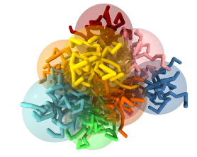
Figure 2: Star polymer molecules (in different colors) in a melt are coarse-grained at the level of their centers of mass. The resulting model is a blob model of the DPD type Hijón et al. (2010).

Static CG is concerned with approximations to the exact potential of mean force that gives, formally, the equilibrium distribution function of all the CG degrees of freedom. Radial distributions, equations of state, et c. are the concern of static coarse graining. There is a vast literature in the construction of the potential of mean force for CG representations of complex fluids Reith et al. (2001); Likos (2001); Voth (2009), and complex molecules Milano and Müller-Plathe (2005); Noid (2013); Lopez et al. (2014). Despite these efforts, there is still much room for improvement in the thermodynamic consistency for the modeling of the potentials of mean force Reinier et al. (2001). If one uses the CG potential for the motion of the CG degrees of freedom, the resulting dynamics is unrealistically fast, although this may be in some cases convenient computationally.

Dynamic CG, on the other hand, focuses on obtaining, in addition to CG potentials, approximations to the friction forces between CG degrees of freedom. Within the theoretical framework of Mori-Zwanzig approach, it is possible to obtain in general the dynamics of the CG degrees of freedom from the underlying Hamiltonian dynamics. The first attempt to derive the DPD model from the underlying microscopic dynamics was given by Español for the simple case of a one dimensional harmonic lattice Español (1996). The center of mass of groups of atoms were taken as the CG variables and Mori’s projection method was used. Because this system is analytically soluble, a flaw in the original derivation could be detected, and an interesting discussion emerged on the issue of non-Markovian effects in solid systems Cubero and Yaliraki (2005a, b); Hijón et al. (2006); Cubero (2008); Hijón et al. (2008).

By following Schweizer Schweizer (1989), Kinjo and Hyodo Kinjo and Hyodo (2007) obtained a formal equation for the centers of mass of groups of atoms. The momentum equation contains three forces, a conservative force deriving from the exact potential of mean force, a friction force and a random force. By modeling the random forces the authors of Ref. Kinjo and Hyodo (2007) showed that this equation encompass both, the BD and DPD equations. However, to consider the procedure in Ref. Kinjo and Hyodo (2007) a derivation of DPD, it is necessary to specify the conditions under which one obtains BD instead of DPD (or vice versa). This was not stated by Kinjo and Hyodo. The crucial insight is that BD appears when “solvent” is eliminated from the description, this is, some (the majority) of the atoms are not grouped and are instead described as a passive thermal bath (or implicit solvent). The friction force in this case is proportional to the velocity of the particles, and the momentum of the CG blobs is not conserved. On the other hand, a DPD description appears when all the atoms are partitioned into disjoint groups. In this case, the conservation of momentum induced by Newton’s third law at the microscopic level leads to a structure of the friction forces depending on relative velocities of the particles. A derivation of the equations of DPD from first principles taking into account linear momentum conservation was presented by Hijon et al. Hijón et al. (2010). The position-dependent friction coefficient was given in terms of a Green-Kubo expression that could be evaluated, under certain simplifying assumptions, directly from MD simulations, within the same spirit of an early derivation of Brownian Dynamics for a dimer representation (non-momentum conserving) of a polymer by Akkermans and Briels Akkermans and Briels (2000). The general approach was preliminarly tested for a system of star polymers (as those in Fig. 2). A subsequent thorough study of this star polymer problem by Karniadakis and co-workers Li et al. (2014) has shown that the introduction of an intrinsic spin variable for each polymer molecule seems to be necessary at low concentrations in order to have an accurate representation of the MD results. The approach in Ref. Hijón et al. (2010) has been labeled by Li et al. Li et al. (2014) as the MZ-DPD approach, standing for Mori-Zwanzig dissipative particle dynamics. Other complex molecules (neopentane, tetrachloromethane, cyclohexane, and n-hexane) have been also considered Deichmann et al. (2014) within the MZ-DPD approach with interesting discussion on the validity of non-Markovian behaviour (more on this later). A slightly more general approach for the derivation of MZ-DPD equations has been given by Izvekov Izvekov (2015). Very recently, Español et al. Español et al. (2016) have formulated from first principles the dynamic equations for an energy conserving CG representation of complex molecules. This work gives the microscopic foundation of the EDPD model for complex molecules (involving bonded atoms only).

V.3 Non-Markov effects

The rigorous coarse-graining in which centers of mass of groups of atoms are used as CG variables relies on a basic and fundamental hypothesis, which is the separation of time scales of the evolution of the CG variables and “the rest” of variables in the system. More accurately, the separation of time scales refers to the existence, in the evolution of the CG variables themselves of two well-defined scales, a large amplitude slow component, and a small high frequency component that can be modeled in terms of white noise. The dynamics of the CG variables can then be approximately described by a non-linear diffusion equation in the space spanned by the CG variables Green (1952); Zwanzig (1961). This separation of time scales does not always exist, either because the groups of atoms are small and the centers of mass momenta evolve in the same time scales as the forces (due to collisions with atoms of other groups) Deichmann et al. (2014), or because of the existence of coupled slow processes not captured by the selected CG variables. When this happens, one strategy is to tweak the friction and simply fit frictions to recover the time scales. Gao and Fang used this approach in order to coarse grain a water molecule to one site-CG particle Gao and Fang (2011). Another strategy is to enlarge the set of CG variables with the hope that the new set will be Markovian. Briels Briels (2009) addresses specifically the problem of CG in polymers and introduces transient forces to recover a Markovian description. Davtyan, Voth, and Anderson Davtyan et al. (2015) have considered the introduction of “fictitious particles” in order to recover the CG dynamics observed from MD. The fictitious particles are just a simple and elegant way to model the memory kernel in a particularly intuitive way. If the strategy to increase the dimension of the CG state space does not work yet, it is still possible to formulate from microscopic principles formal non-Markovian models and to extract information about the memory kernel from MD Yoshimoto et al. (2013). However, in the absence of separation of time scales, the computational effort required to get from MD the memory kernel makes the whole strategy of bottom-up coarse graining inefficient. Note that the advantage of a bottom-up strategy for coarse graining is that one needs to run relatively short MD simulations to get the information (Green-Kubo coefficients) that is used in the dynamic equations governing much larger time scales. If one needs to run long MD simulation of the microscopic system to get the CG information, we have already solved the problem by brute force in the first place!

V.4 Electrostatic interactions

In many situations, one is interested in the consequential effects of charge separation. This is particularly so for aqueous systems where the relatively high dielectric permittivity of water means that ion dissociation readily occurs. The relevance lies not only in the structural and thermodynamic properties of ionic surfactants and polyelectrolytes et c, Šindelka et al. (2014); Lísal et al. (2016) but is also motivated by a burgeoning interest of electrokinetic phenomena Pagonabarraga et al. (2010); Smiatek and Schmid (2012); Maduar et al. (2015); Sepehr and Paddison (2016).

An important point to make is that some relevant electrostatic effects simply cannot be captured in a short-range interaction (DPD-like or otherwise). For example the bare electrostatic energy of a charged spherical micelle of aggregation number $N$ scales as $N^{2}/R\sim N^{5/3}$, where $R\sim N^{1/3}$ is the micelle radius. This electrostatic energy cannot be captured in either a volume ($\sim N$) or surface ($\sim N^{2/3}$) term. To be faithful to this physics therefore, one has in some way to incorporate long-range Coulomb interactions explicitly into the DPD model. This area was pioneered by Groot, who used a field-based method Groot (2003). Since then, more standard Ewald methods have also been used González-Melchor et al. (2006); Warren et al. (2013), and in principle any fast electrostatics solver developed for MD could be taken over into the DPD domain. One important caveat is that with soft particles (ie no hard core repulsion) the singularity of Coulomb interactions needs to be tamed through the use of smoothed charge models Groot (2003); González-Melchor et al. (2006); Warren et al. (2013); Warren and Vlasov (2014). Adding electrostatics is certainly computationally expensive, often halving the speed of DPD codes. This drastic slow-down offsets the advantage of the DPD methods when compared to more traditional coarse-graining methods.

Related to the problem of charge separation is the question of dielectric inhomogeneities (image charges et c), such as encountered in oil/water mixtures and at interfaces. In field-based methods this can be resolved by having a local-density-dependent dielectric permittivity Groot (2003). Alternatively one can introduce an explicitly polarisable solvent model Peter and Pivkin (2014); Peter et al. (2015). Note that an electric field in the presence of a dielectric inhomogeneity induces reaction forces on the uncharged particles Groot (2003). In a field-based method, this is quite complicated to incorporate in a rigorous way. For an explicitly polarisable solvent model, these induced reaction forces of course arise naturally and are automatically captured.

VI Systems studied with DPD

The number of systems and problems that have been addressed with DPD or its variants is enormous and we do not pretend to review the extensive literature on the subject. Nevertheless, to illustrate the range and variety of different applications of DPD we give a necessarily brief survey of the field. A general trend observed in the application side, is the shift from the original DPD model, of “balls and springs” models, towards more specific atomistic detail, in the line of MZ-DPD, or semi-bottom-up DPD (with structure based CG potentials and fitted friction).

Colloids: A recent review on the simulation of colloidal suspensions with particle methods, including DPD, can be found in Bolintineanu et al. (2014). The first application of DPD to a complex fluid was the simulation of colloidal rheology by Koelman and Hooggerbruge Koelman and Hoogerbrugge (1993). Since then, a large number of works have addressed the simulation of colloidal suspensions, with a variety of approaches to represent the solute. Typically, a colloidal particle is constructed out of dissipative particles that are moved rigidly Koelman and Hoogerbrugge (1993); Li and Drazer (2008), or connected with springs Laradji and Hore (2004); Phan-Thien et al. (2014). Arbitrary shapes may be considered in this way Boek et al. (1997), as well as confinement due to walls Gibson et al. (1999); Li and Drazer (2008). As a way to bypass the need to update the relatively large number of solid particles, some approaches represent each colloidal particle with a single dissipative particle Pryamitsyn and Ganesan (2005); Pan et al. (2008, 2010), leading to minimal spherical blob models for the colloids. These simplified models for the solute require the introduction of shear forces of the FPM type. Representing a colloidal particle with a point particle is a strategy also used in minimal blob models in Eulerian CFD methods for fluctuating hydrodynamics Balboa Usabiaga et al. (2014). A core can be added in order to represent hard spheres with finite radii, supplemented with a dissipative surface to mimic boundary conditions Whittle and Travis (2010), and still retain the one-particle-per-colloid scheme. Although general features show semi-quantitative agreement with experimental results Whittle and Travis (2010), other simulation techniques like Stokesian Dynamics, and theoretical work, it is clear that getting more detailed physics of colloid-colloid interactions and colloid-solvent interaction (either through a MZ-DPD approach or by phenomenologically including boundary layers and top-down parametrization) may be beneficial to the field.

Blood: A colloidal system of obvious biological interest is blood. Blood has been simulated with DPD Fedosov et al. (2011), and more recently with SDPD Moreno et al. (2013); Müller et al. (2014); Katanov et al. (2015). Two recent reviews Li et al. (2013); Ye et al. (2015) discuss the modeling of blood with particle methods. Multi-scale modeling (i. e. MZ-DPD) seems to be crucial to capture platelet activation and thrombogenesis Zhang et al. (2014).

Polymers: An excellent recent review on coarse-graining of polymers is given by Padding and Briels Padding and Briels (2011). Below the entanglement threshold Rouse dynamics holds and this is well satisfied in a DPD polymer melt Spenley (2000). Above the threshold, entanglements are a necessary ingredient in polymer melts. Because the structure based CG potential between the blobs are very soft, it is necessary to include a mechanism for entanglement explicitly. This is one example in which the usual simple schemes to treat the many-body potential (through pair-wise interactions) fails dramatically. There are several methods to include entanglements: Padding and Briels Padding and Briels (2001, 2002) introduced the elastic band method for coarse-grained simulations of polyethylene. Another alternative to represent entanglements is to use the Kumar and Larson method Kumar and Larson (2001); Goujon et al. (2008); Yamanoi et al. (2011) in which a repulsive potential between bonds linking consecutive blobs is introduced. Finally, entanglements can be enforced in a simpler way by hard excluded volume LJ interactions Symeonidis et al. (2005), or through suitable criterion on the stretching of two bonds and the amount of impenetrability of them Nikunen et al. (2007).

Beyond scaling properties, effort has been directed towards a chemistry detailed MZ-DPD methodology, by using structure based CG effective potentials and either fitting the friction coefficient Guerrault et al. (2004); Lahmar and Rousseau (2007); Maurel et al. (2012, 2015), or obtaining the dissipative forces from Green-Kubo expressions Trément et al. (2014). In general, one can take advantage of systematic static coarse-graining approaches, like those for heptane and toluene Dunn and Noid (2015), to be directly incorporated to DPD. Very recently, new Bayesian methods for obtaining the CG potential and friction are being considered Dequidt and Solano Canchaya (2015); Solano Canchaya et al. (2016) (on pentane). The ultimate goal of all these microscopically informed approaches is to predict rheological properties as a function of chemical nature of the polymer system with a small computational cost. As mentioned earlier, whatever improvement in the construction of CG potentials will be highly beneficial also for the construction of dynamic CG models. In this respect, the work on analytical integral equation approach of Guenza and co-workers McCarty et al. (2014) for obtaining the CG potential in polymer systems that ensures both, structural properties and thermodynamic behaviour seems to be very promising.

We perceive a powerful trend towards more microscopically informed DPD able to express faithfully the chemistry of the system. This trend is important when considering hierarchical multi-scale methods in which MD information is transferred to a dynamic CG DPD model, the DPD model is evolved in order to get topology and equilibrium states much faster than MD, and then a back-mapping fine grained procedure recovers microscopic states able to be evolved again with MD Chen et al. (2006b); Santangelo et al. (2007); Gavrilov et al. (2015).

Other complex fluid systems involving polymers have been considered. An early work is the study of adsorption of colloidal particles onto a polymer coated surface Gibson et al. (1999). Polymer brushes are reviewed by Kreer Kreer (2016). Self assembly of giant amphiphiles made of a nanoparticle with tethered polymer tail has been considered recently Ma et al. (2015). Polymer membranes for fuel cells have been considered by Dorenbos Dorenbos (2015). Polymer solutions simulated with DPD obey Zimm theory that includes hydrodynamic interactions Jiang et al. (2007). Polymer solutions have also been studied with SDPD observing Zimm dynamics Litvinov et al. (2008).

Phase separating fluids: In polymer mixtures, the $\chi$-parameter mapping introduced by Groot and Madden Groot and Madden (1998) has been phenomenally popular because it links to long-established polymer physical chemistry (there are tables of $\chi$-parameters for instance, and a large literature devoted to calculating $\chi$-parameters ab initio). This has helped incorporate chemical specificity in DPD from solubility parameters Maiti and McGrother (2004); Liyana-Arachchi et al. (2015). It is also known that $\chi$-parameters can be composition dependent (PEO in water is the notorious example). This can be accommodated within the MDPD approach. Akkermans Akkermans (2008) presents a first principles coarse-graining method that allows to calculate the excess free energy of mixing and Flory-Huggins $\chi$-parameter. A related effort is given by Goel et al. Goel et al. (2014).

DPD has been very successful in identifying mechanisms in phase separation: Linear diblock copolymer spontaneously form a mesocopically ordered structure (lamellar, perforated lamellar, hexagonal rods, micelles) Groot and Madden (1998). DPD is capable to predict the dynamical pathway towards equilibrium structures and it is observed that hydrodynamic interactions play an important role in the evolution of the mesophases Groot et al. (1999). Domain growth and phase separation of binary immiscible fluids of differing viscosity was studied in Novik and Coveney (2000). New mechanisms via inertial hydrodynamic bubble collapse for late-stage coarsening in off-critical vapor-liquid phase separation have been identified Warren (2001). The effect of nanospheres in the mechanisms for domain growth in phase separating binary mixture has been considered by Laradji and Hore Laradji and Hore (2004).

Drop dynamics: A particular case of phase separating fluids is given by liquid-vapour coexistence giving rise to droplets. Surface-confined drops in a simple shear was studied in an early work Jones et al. (1999). Pendant drops have been studied with MDPD Warren (2003a), while oscillating drops Liu et al. (2006), and drops on superhydrophobic substrates Wang and Chen (2015), have also been considered.

Amphiphilic systems: An early review of computer modeling of surfactant systems is by Shelley and Shelley Shelley and Shelley (2000). A more recent review on the modeling of pure membranes and lipid-water membranes with DPD is given by Guigas et al. Guigas et al. (2011). Coarsening dynamics of smectic mesophase of amphiphilic species for a minimal amphiphile model was studied by Jury et al. Jury et al. (1999b) and mesophase formation in pure surfactant and solvent by Prinsen et al. Prinsen et al. (2002). More microscopic detail has been included by Ayton and Voth Ayton and Voth (2002) with DPD model for CG lipid molecules that self assembly, a problem also considered by Kranenburg and Venturoli Kranenburg and Venturoli (2003). Effort towards more realistic parametrization for lipid bilayers was given by Gao et al. Gao et al. (2007). Prior to this Li et al. Li et al. (2004) formulated a conservative force derived from a bond-angle dependent potential that allowed to consider different types of micellar structures. Microfluidic synthesis of nanovesicles was considered by Zhang et al. Zhang et al. (2015a). Simulations of micelle-forming systems have also been reported Vishnyakov et al. (2013); Johnston et al. (2016).

Oil industry: DPD simulations have also addressed problems in the oil industry, from oil-water-surfactant dynamics Rekvig et al. (2004), and water-benzene-caprolactam systems Shi et al. (2015), to aggregate behavior of asphaltenes in heavy crude oil Zhang et al. (2010), or the orientation of asphaltene molecules at the oil-water interface Ruiz-Morales and Mullins (2015).

Biological membranes: A review of mesoscopic modeling of biological membranes was given by Venturoli et al. Venturoli et al. (2006). Groot and Rabone Groot and Rabone (2001) presented one of the first applications of DPD to the modeling of biological membranes and its disruption due to nonionic surfactants. Sevink and Fraaije Sevink and Fraaije (2014) devised a coarse-graining of a membrane into a DPD model in which the solvent was treated implicitly. Amphiphilic polymer coated nanoparticles for assisted drug delivery through cell membranes has been recently studied Zhang et al. (2015b, c). The diffusion of membrane proteins has been considered iby Guigas and Weiss Guigas and Weiss (2015).

Biomolecular modeling: The CG modeling of complex biomolecules with a focus on static properties has been addressed in the excellent review by Noid Noid (2013). Pivkin et al. Peter et al. (2015) have modeled proteins with DPD force fields, which competes with the Martini force field Marrink and Tieleman (2013).

Inorganic materials: DPD has also been used for the CG modeling of solid inorganic materials. Coarse-grained representation of graphene turns out to be essential for study of large scale resonator technology Kauzlarić et al. (2011a, b).

VII Conclusions

The DPD model is a tool for simulating the mesoscale. The model has evolved since its initial formulation towards enriched models that, while retaining the initial simplicity of the original, are now linked strongly to either the microscopic scale or the macroscopic continuum scale. In many respects, the original DPD model of Fig. 1 is a toy model and one can do much better by using these refined models. In this Perspective, we wish to convey the message that DPD has a dual role in modeling the mesoscale. It has been used as a way to simulate, on one hand, coarse-grained (CG) versions of complex molecular objects and, on the other hand, fluctuating fluids. While the first type of application, involving atoms bonded by their interactions, has a solid ground on the theory of coarse graining, there is no such a microscopic basis for DPD as a fluid solver. The best we can do today is to descend from the continuum theory and to formulate DPD as a Lagrangian discretization of fluctuating hydrodynamics, leading to the SDPD model.

Therefore as DPD simulators we are faced with three alternative strategies:

#1 Bottom-up MZ-DPD: When dealing with molecular objects made of bonded atoms, we may formulate an appropriate CG mapping and construct the DPD equations of motion with momentum conserving forces Hijón et al. (2010). These equations contain the potential of mean force generating conservative forces and position-dependent friction coefficient, with explicit microscopic formulae: the potential of mean force is given by the configuration dependent free energy function, and the position dependent friction coefficient tensor is given by Green-Kubo expressions. Both quantities are given in terms of expectations conditional on the CG variables and are, therefore, many-body functions. These are not, in general, directly computable due to the curse of dimensionality. One needs to formulate simple and approximate models (usually pair-wise with, perhaps, bond-angle and torsion effects) in order to represent the complex functional dependence of these quantities. Together with the initial selection of the CG mapping, finding suitable functional forms is the most delicate part of the problem. Once this simple functional models are selected, constrained MD simulations Akkermans and Briels (2000); Hijón et al. (2010), or optimization methods Noid (2013); Brini et al. (2013); Lopez et al. (2014); Dequidt and Solano Canchaya (2015), may be used to obtain the CG potential.

The existence of a framework to derive dynamic CG models from bottom-up is a highly rewarding intellectual experience with a high practical value because 1) it provides the structure of the dynamic equations, and 2) signals at the crucial points where approximations are required. The MZ-DPD approach is, in our view, an important breakthrough in the field, as it connects the well established world of static coarse-graining with the DPD world Noid (2013). In this way, it provides a framework for accurately addressing the CG dynamics. However, the usefulness to follow the program by the book is not always obvious due to the large effort in obtaining the objects form MD. In this case, one would go to the next strategy.

#2 Parametrization of DPD: We may insist on a particularly simple form of linear repulsive forces and simple friction coefficients (like the ones in the original/cartoon DPD model) and fit the parameters to whatever property of the system one wants to correctly describe (for example, the compressibility). Nowadays, we advise caution with this simple approach because, usually, many other properties of the system go wrong. The simple DPD linear forces are not flexible enough in many situations. However, from what we have already learned from microscopically informed MZ-DPD in the previous #1 strategy, we may give ourselves more freedom in selecting the functional forms (as in MDPD) for conservative and friction forces and have more free parameters to play with. Once it is realized that the potential between beads or blobs in DPD is, in fact, the potential of mean force, one can use semi-bottom-up approaches in which the potential of mean force is obtained from first principles, while the DPD friction forces are fitted to obtain the correct time scales Lyubartsev et al. (2002); Guerrault et al. (2004); Lahmar and Rousseau (2007). Although this strategy is less rigorous, it may be more practical in some cases.

The #1 bottom-up MZ-DPD strategy above has not been yet successful when the interactions of atoms or molecules in the system are unbonded, allowing two molecules that are initially close together to diffuse away from each other. These are the kind of interactions present in a fluid system. The main difficulty seems to be in the Lagrangian nature of a fluid particle that makes the CG mapping not obvious. Although some attempts have been taken in order to derive DPD for fluid systems with unbonded interactions, we believe that the problem is not yet solved. However, for these systems one may regard the dissipative particles as truly fluid particles (i. e.  small thermodynamic systems that move with the flow). We are lead to the third strategy.

#3 Top-down DPD: Assume that we know that a particular field theory describes the complex fluid of interest at a macroscopic scale (Navier-Stokes for a Newtonian fluid, for example). Then one may discretize the theory on moving Lagrangian points according to the SPH mesh-free methodology. The Lagrangian points may be interpreted as fluid particles. If we perform this discretization within a thermodynamically consistent framework like generic Öttinger (2005), thermal fluctuations are automatically determined correctly Petsev et al. (2016), allowing to address the mesoscale. This strategy leads to enriched DPD models (SDPD is an example corresponding to Navier-Stokes hydrodynamics). The functional forms of conservative and friction forces in this DPD models are dictated by the mesh-free discretization, as well as the input information of the field theory itself. We have the impression that SDPD or its isothermal counterpart MDPD are underappreciated and underused. Although these methods are appropriate for fluid systems, we foresee the use of MDPD many-body potentials of the embedded atom form also for CG potentials for bonded atom systems. While CG potentials depending on the global density are potentially a trap Louis (2002); D’Adamo et al. (2013), the inclusion of many-body functional forms of the embedded atom kind depending on local density is a promissing route to have more transferable CG potentials Allen and Rutledge (2008), valid for different thermodynamic points. This expectation, though, needs to be substantiated by further research. In particular, liquid state theory for MDPD may need to be further developed Merabia and Pagonabarraga (2007); McCarty et al. (2014).

This Perspective on DPD also points to several open methodological questions.

We have already mentioned the open problem of deriving from microscopic principles the dynamics of Lagrangian fluid particles made of unbonded atoms. Once this problem is solved, we will need to face the next problem of deriving from first principles the coupling of CG descriptions of bonded and unbonded atoms (a protein in a membrane surrounded by a solvent, for example). A derivation from bottom-up of this kind of coupling in a discrete Eulerian setting has been given recently in Español and Donev (2015).

For the simulation of fluids, standard CFD methods equipped with thermal fluctuations are readily catching up with the mesoscale Naji et al. (2009); Uma et al. (2011); Shang et al. (2012); Donev et al. (2010); Oliver et al. (2013); Donev and Vanden-Eijnden (2014); Donev et al. (2014); Plunkett et al. (2014); De Corato et al. (2016). Methods for coupling solvents and suspended structures are being devised Balboa Usabiaga et al. (2014); Español and Donev (2015), and therefore one may well ask what is the advantage of a Lagrangian solver based on the relatively inaccurate SPH discretization over these high quality CFD methods. Note that CFD methods allow for the rigorous treatment of limits (incompressibility, inertia-less, et c) that may imply large computer savings, and which are difficult to consider in SPH based methods. We believe (see Meakin and Xu Meakin and Xu (2009) for a defense of particle methods) that fluid particle models may still compete in situations where biomolecules and other complex molecular structures move in solvent environments, because one does not need to change paradigm: only particles for both, solvent and beads, are used, with the corresponding simplicity in the codes to be used. Nevertheless, a fair comparison between Eulerian and Lagrangian methodologies is still missing.

As SDPD is just SPH plus thermal fluctuations it inherits the shortcomings of SPH itself. SPH is still facing some challenges in both, foundations (boundary conditions) and computational efficiency Violeau and Rogers (2016); Wang et al. (2016). In this respect, a Voronoi fluid particle model Serrano and Español (2001), understood as a Lagrangian finite volume solver may be an interesting possibility both in terms of computational efficiency and simplicity of implementation of boundary conditions. Serrano compared SDPD and a particular implementation in 2D of Voronoi fluid particles Serrano (2006). In terms of computational efficiency, both methods are comparable because the extra cost in computing the tessellation is compensated by the small number of neighbours required, six on average, while in SDPD one needs 20-30 neighbours.

Another interesting area of research is that of multi-scale modeling. In CFD, one way to reduce the computational burden is to increase the resolution of the mesh only in those places where strong flow variations occur, or interesting molecular physics requiring small scale resolution is taking place. An early attempt within DPD was given by Backer et al. Backer et al. (2005). We envisage that methods for multi-resolution SDPD will be increasingly used in the future Kulkarni et al. (2013); Lei et al. (2015); Tang et al. (2015); Petsev et al. (2016). Multi-resolution is a problem of active research also in the SPH community Violeau and Rogers (2016). Eventually, one would like to hand-shake the particle method of SDPD with MD as the resolution is decreased Petsev et al. (2015). Note, however, that as the fluid particles become small (say “four atoms per particle”) it is expected that the Markovian property breaks down and one needs to account for viscoelasticity Zwanzig and Bixon (1975); Voulgarakis and Chu (2009), either with additional internal variables ten Bosch (1999); Ellero et al. (2003); Vázquez-Quesada et al. (2009b), or with “fictitious particles” Davtyan et al. (2015).

Finally, a very interesting research avenue is given by the thermodynamically consistent (i. e., able to deal with non-isothermal situations) Mori-Zwanzig EDPD introduced theoretically by Español et al. Español et al. (2016). Up to now, CG representations of complex molecules have only included the location and velocity of the CG beads or blobs (sometimes its spin Li et al. (2014)), completely forgeting its internal energy content. Given the fundamental importance of the principle of energy conservation, it seems that in order to have thermodynamically consistent and more transferable potentials, we may need to start looking at these slightly more complex CG representations.

VIII Acknowledgments

We acknowledge A. Donev for useful comments on the manuscript. PE thanks the Ministerio de Economía y Competitividad for support under grant FIS2013-47350-C5-3-R.

Appendix A MDPD consistency

In MDPD the potential takes the form described in the main text where $V(\{{\mathbf{r}}\})=\sum_{i}\psi(d_{i})$, and $d_{i}=\sum_{j\neq i}W(r_{ij})$. From this it is easy to show that the forces remain pairwise, with

$${\mathbf{F}}_{ij}=-[\psi^{\prime}(d_{i})+\psi^{\prime}(d_{j})]\,W^{\prime}(r_{ij})\,{\mathbf{e}}_{ij}\,.$$ (5)

Note that the weight function here is $W^{\prime}(r)$. However, to our knowledge, there does not exist in the literature a proof of the converse, namely that this relationship between the weight functions is a necessary condition to ensure the existence of $V(\{{\mathbf{r}}\})$. We present here such a proof, following the line of argument in Ref. Warren (2013).

We start with a generalised MDPD pairwise force law, with an (as yet) arbitrary weight function $\omega^{c}(r)$,

$${\mathbf{F}}_{ij}=A(d_{i},d_{j})\,\omega^{c}(r_{ij})\,{\hat{\mathbf{r}}}_{ij}\,.$$ (6)

We assume the amplitude function $A(d_{i},d_{j})$ is symmetric since otherwise ${\mathbf{F}}_{ij}\neq-{\mathbf{F}}_{ji}$. Let us denote partial derivatives with respect to the first and second density arguments by $A_{[1,0]}$ and $A_{[0,1]}$. The symmetry of $A(d_{i},d_{j})$ then implies $A_{[1,0]}(d_{i},d_{j})=A_{[0,1]}(d_{j},d_{i})$.

A generic radial force law can always be integrated, so we cannot deduce anything useful just by considering pairs of particles. Instead, following Ref. Warren (2013), let us consider three isolated, collinear particles, at positions $x_{i}$ ($i=1\dots 3$) such that $x_{1}\leq x_{2}\leq x_{3}$. For this configuration the densities are $d_{1}=W(x_{12})+W(x_{13})$, $d_{2}=W(x_{12})+W(x_{23})$, and $d_{3}=W(x_{13})+W(x_{23})$. The pairwise forces are $F_{12}=A(d_{1},d_{2})\,\omega^{c}(x_{12})$, $F_{23}=A(d_{2},d_{3})\,\omega^{c}(x_{23})$, and $F_{13}=A(d_{1},d_{3})\,\omega^{c}(x_{13})$. Finally, the summed forces on the particles are $F_{1}=F_{12}+F_{13}$, $F_{2}=-F_{12}+F_{23}$, and $F_{3}=-F_{13}-F_{23}$.

The existence of a potential implies integrability constraints like $\partial F_{1}/\partial x_{2}-\partial F_{2}/\partial x_{1}=0$. Imposing these gives rise to an expression which can be simplified (by consideration of special cases) to a set of requirements for which the representative case is

$$\begin{split}&\omega^{c}(x_{12})\,W^{\prime}(x_{23})\,A_{[1,0]}(d_{1}+d_{3},d_{1})\\ &\qquad-\omega^{c}(x_{23})\,W^{\prime}(x_{12})\,A_{[1,0]}(d_{1}+d_{3},d_{3})=0.\end{split}$$ (7)

The symmetry relation between $A_{[0,1]}$ and $A_{[1,0]}$ has been used. If we are allowed to cancel the $A_{[1,0]}$ functions we are home and dry, since this implies $\omega^{c}(x)\,W^{\prime}(y)=\omega^{c}(y)\,W^{\prime}(x)$ (for arbitrary arguments $x$ and $y$), and this can only be true if $\omega^{c}(x)\propto W^{\prime}(x)$. However, the $A_{[1,0]}$ functions only cancel if $A_{[1,0]}(x+y,x)=A_{[1,0]}(x+y,y)$ (for arbitrary arguments $x$, $y$). A little thought shows that a sufficient condition for this to be true is that $A(d_{i},d_{j})=f(d_{i})+f(d_{j})$. This is precisely the form the force-law takes in Eq. (5). The conclusion is that in this case $\omega^{c}(x)\propto W^{\prime}(x)$ is a necessary condition for the existence of the many-body potential $V(\{{\mathbf{r}}\})$. It is also sufficient, since we can absorb the proportionality constant into the definitions of $d_{i}$ and $\psi(d)$, and then explicitly $V(\{{\mathbf{r}}\})=\sum_{i}\psi(d_{i})$. This proves the claimed result above.

For another example, we might be tempted to consider $A(d_{i},d_{j})=f(d_{i}+d_{j})$, but retaining the weight function $\omega^{c}(x)\propto W^{\prime}(x)$. For this choice $A_{[1,0]}(x,y)=f^{\prime}(x+y)$ and Eq. (7) reduces to $f^{\prime}(2x+y)=f^{\prime}(x+2y)$. This is true for arbitrary $x$ and $y$ if only if $f(x)$ is linear, and therefore the force law is de facto of the form shown in Eq. (5). Thus, a non-linear function $f(x)$ would be a bad choice. For a further case study, see Ref. Warren (2013).

If we fail to satisfy Eq. (7) then the potential does not exist. If the potential does not exist, we lose the underpinning theory that the stationary probability distribution is given by Eq. (2). Without this foundation we are in uncharted waters, and there is no link to established statistical mechanics and thermodynamics.

In our opinion, in MDPD the burden rests on the user to display the $V(\{{\mathbf{r}}\})$ which gives rise to the chosen force law. The absence of an explicitly displayed potential leads only to unwarranted complications.

References

- Berendsen (2007) H. J. C. Berendsen, Simulating the Physical World: Hierarchical Modeling from Quantum Mechanics to Fluid Dynamics (Cambridge University Press, Cambridge, UK, 2007).
- Heinecke et al. (2015) A. Heinecke, M. Horsch, and W. Eckhardt, Supercomputing for Molecular Dynamics Simulations. Handling Multi-Trillion Particles in Nanofluidics (Springer, Berlin, Germany, 2015).
- Shillcock (2008) J. C. Shillcock, HFSP J. 2, 1 (2008).
- Öttinger (2005) H. C. Öttinger, Beyond Equilibrium Thermodynamics (J. Wiley & Sons, Hoboken, NJ, 2005).
- Batchelor (1967) G. K. Batchelor, An Introduction to Fluid Dynamics (Cambridge University Press, Cambridge, UK, 1967).
- de Groot and Mazur (1964) S. R. de Groot and P. Mazur, Non-Equilibrium Thermodynamics (North Holland, Amsterdam, The Netherlands, 1964).
- Alder and Wainwright (1970) B. J. Alder and T. E. Wainwright, Phys. Rev. A 1, 18 (1970).
- Landau and Lifshitz (1959) L. D. Landau and E. M. Lifshitz, Fluid Mechanics (1st edn) (Pergamon, Oxford, UK, 1959).
- Naji et al. (2009) A. Naji, P. J. Atzberger, and F. L. H. Brown, Phys. Rev. Lett. 102, 138102 (2009).
- Uma et al. (2011) B. Uma et al., Phys. Fluids 23, 073602 (2011).
- Shang et al. (2012) B. Z. Shang, N. K. Voulgarakis, and J.-W. Chu, J. Chem. Phys. 137, 044117 (2012).
- Donev et al. (2010) A. Donev, E. Vanden-Eijnden, A. L. Garcia, and J. B. Bell, Commun. Appl. Math. Comput. Sci. 5, 149 (2010).
- Oliver et al. (2013) R. C. Oliver, D. J. Read, O. G. Harlen, and S. A. Harris, J. Comput. Phys. 239, 147 (2013).
- Donev and Vanden-Eijnden (2014) A. Donev and E. Vanden-Eijnden, J. Chem. Phys. 140, 234115 (2014).
- Donev et al. (2014) A. Donev, T. G. Fai, and E. Vanden-Eijnden, J. Stat. Mech.: Theory Exp. 2014, P04004 (2014).
- Plunkett et al. (2014) P. A. T. Plunkett, J. O. N. Hu, C. Siefert, and P. J. Atzberger, J. Comput. Phys. 277, 121 (2014).
- De Corato et al. (2016) M. De Corato et al., J. Comput. Phys. 316, 632 (2016).
- Voth (2009) G. A. Voth, ed., Coarse-Graining of Condensed Phase and Biomolecular Systems (CRC Press, Boca Raton, FL, 2009).
- Noid (2013) W. G. Noid, J. Chem. Phys. 139, 090901 (2013).
- Brini et al. (2013) E. Brini et al., Soft Matter 9, 2108 (2013).
- Lopez et al. (2014) C. A. Lopez et al., WIREs Comput. Mol. Sci. 4, 225 (2014).
- Green (1952) M. S. Green, J. Chem. Phys. 20, 1281 (1952).
- Zwanzig (1961) R. Zwanzig, Phys. Rev. 124, 983 (1961).
- Grabert (1982) H. Grabert, Projection Operator Techniques in Nonequilibrium Statistical Mechanics (Springer, Berlin, Germany, 1982).
- Zubarev D. (1996) R. G. Zubarev D., Morozov V., Statistical Mechanics of Nonequilibrium Processes: Basic Concepts, Kinetic Theory (Akademie Verlag, Berlin, Germany, 1996).
- Español (2004) P. Español, in Novel Methods in Soft Matter Simulations, edited by M. Karttunen, I. Vattulainen, and A. Lukkarinen (Springer, Berlin, Germany, 2004), pp. 2256–2256.
- Malevanets and Kapral (1999) A. Malevanets and R. Kapral, J. Chem. Phys. 110, 8605 (1999).
- Succi (2001) S. Succi, The Lattice Boltzmann Equation for Fluid Dynamics and Beyond (Oxford University Press, Oxford, UK, 2001).
- Holm and Kremer (2009) C. Holm and K. Kremer, eds., Advanced Computer Simulation Approaches for Soft Matter Sciences III (Springer, Berlin, Germany, 2009).
- Dünweg and Ladd (2009) B. Dünweg and A. J. C. Ladd, in Holm and Kremer (2009), pp. 89–166.
- Gompper et al. (2009) G. Gompper, T. Ihle, D. M. Kroll, and R. G. Winkler, in Holm and Kremer (2009), pp. 1–87.
- Donev et al. (2009) A. Donev, B. J. Alder, and A. L. Garcia, J. Stat. Mech.: Theory Exp. 2009, P11008 (2009).
- Warren (1998) P. B. Warren, Curr. Opin. Colloid Interface Sci. 3, 620 (1998).
- Pivkin et al. (2010) I. V. Pivkin, B. Caswell, and G. E. Karniadakis, in Rev. Comput. Chem., edited by K. B. Lipkowitz (J. Wiley & Sons, Hoboken, NJ, 2010), vol. 27, pp. 85–110.
- Moeendarbary et al. (2010) E. Moeendarbary, T. Y. Ng, and M. Zangeneh, Int. J. Appl. Mech. 2, 161 (2010).
- Guigas et al. (2011) G. Guigas, D. Morozova, and M. Weiss, Adv. Protein Chem. Struct. Biol. 85, 143 (2011).
- Lu and Wang (2013) Z.-Y. Lu and Y.-L. Wang, Methods Mol. Biol. 924, 617 (2013).
- Ghoufi et al. (2013) A. Ghoufi, J. Emile, and P. Malfreyt, Eur. Phys. J. E 36, 10 (2013).
- Liu et al. (2014) M. B. Liu, G. R. Liu, L. W. Zhou, and J. Z. Chang, Arch. Comput. Methods Eng. 22, 529 (2014).
- Brennan and Lísal (2009) J. K. Brennan and M. Lísal, Mol. Simul. 35, 766 (2009).
- Mousseau and Montréal (2014) N. Mousseau and U. D. Montréal, Tech. Rep., CECAM (2014).
- Hoogerbrugge and Koelman (1992) P. J. Hoogerbrugge and J. M. V. A. Koelman, Europhys. Lett. 19, 155 (1992).
- Español and Warren (1995) P. Español and P. Warren, Europhys. Lett. 30, 191 (1995).
- Español (1995) P. Español, Phys. Rev. E 52, 1734 (1995).
- Marsh et al. (1997) C. Marsh, G. Backx, and M. Ernst, Phys. Rev. E 56, 1676 (1997).
- Boromand et al. (2015) A. Boromand, S. Jamali, and J. M. Maia, Comput. Phys. Commun. 196, 149 (2015).
- Groot and Warren (1997) R. D. Groot and P. B. Warren, J. Chem. Phys. 107, 4423 (1997).
- Pagonabarraga and Hagen (1998) I. Pagonabarraga and M. Hagen, Europhys. Lett. 377, 377 (1998).
- Shardlow (2003) T. Shardlow, SIAM J. Sci. Comput. 24, 1267 (2003).
- Nikunen et al. (2003) P. Nikunen, M. Karttunen, and I. Vattulainen, Comput. Phys. Commun. 153, 407 (2003).
- Defabritiis et al. (2006) G. Defabritiis, M. Serrano, P. Español, and P. V. Coveney, Physica A 361, 429 (2006).
- Serrano et al. (2006) M. Serrano, G. Defabritiis, P. Español, and P. V. Coveney, Math. Comput. Simul. 72, 190 (2006).
- Thalmann and Farago (2007) F. Thalmann and J. Farago, J. Chem. Phys. 127, 124109 (2007).
- Chaudhri and Lukes (2010) A. Chaudhri and J. R. Lukes, Phys. Rev. E 81, 026707 (2010).
- Litvinov et al. (2010) S. Litvinov, M. Ellero, X. Y. Hu, and N. A. Adams, J. Comput. Phys. 229, 5457 (2010).
- Leimkuhler and Shang (2015) B. Leimkuhler and X. Shang, J. Comput. Phys. 280, 72 (2015).
- Farago and Grønbech-Jensen (2016) O. Farago and N. Grønbech-Jensen, J. Chem. Phys. 144, 084102 (2016).
- Jury et al. (1999a) S. I. Jury, P. Bladon, S. Krishna, and M. E. Cates, Phys. Rev. E 59, R2535 (1999a).
- Keaveny et al. (2005) E. E. Keaveny, I. V. Pivkin, M. Maxey, and G. E. Karniadakis, J. Chem. Phys. 123, 104107 (2005).
- Chen et al. (2006a) S. Chen, N. Phan-Thien, B. C. Khoo, and X. J. Fan, Phys. Fluids 18, 103605 (2006a).
- van de Meent et al. (2008) J.-W. van de Meent et al., Phys. Rev. E 78, 015701 (2008).
- Tiwari et al. (2008) A. Tiwari, H. Reddy, S. Mukhopadhyay, and J. Abraham, Phys. Rev. E 78, 016305 (2008).
- Steiner et al. (2009) T. Steiner, C. Cupelli, R. Zengerle, and M. Santer, Microfluid. Nanofluidics 7, 307 (2009).
- Filipovic et al. (2011) N. Filipovic, M. Kojic, and M. Ferrari, Microfluid. Nanofluidics 10, 1127 (2011).
- Kadau et al. (2010) K. Kadau et al., Philos. Trans. A. Math. Phys. Eng. Sci. 368, 1547 (2010).
- Louis et al. (2000) A. A. Louis, P. G. Bolhuis, and J. P. Hansen, Phys. Rev. E 62, 7961 (2000).
- Warren et al. (2013) P. B. Warren, A. Vlasov, L. Anton, and A. J. Masters, J. Chem. Phys. 138, 204907 (2013).
- Warren and Vlasov (2014) P. B. Warren and A. Vlasov, J. Chem. Phys. 140, 084904 (2014).
- Fraaije et al. (2016) J. G. E. M. Fraaije, J. van Male, P. Becherer, and R. S. Gracià, J. Chem. Inf. Model (2016), article ASAP.
- Trofimov et al. (2002) S. Y. Trofimov, E. L. F. Nies, and M. A. J. Michels, J. Chem. Phys. 117, 9383 (2002).
- Español (1997a) P. Español, Europhys. Lett. 39, 605 (1997a).
- Español (1998) P. Español, Phys. Rev. E 57, 2930 (1998).
- Masters and Warren (1999) A. Masters and P. Warren, Europhys. Lett. 48, 1 (1999).
- Evans (1999) G. Evans, J. Chem. Phys. 110, 1338 (1999).
- Füchslin et al. (2009) R. M. Füchslin, H. Fellermann, A. Eriksson, and H.-J. Ziock, J. Chem. Phys. 130, 214102 (2009).
- Arienti et al. (2011) M. Arienti, W. Pan, X. Li, and G. E. Karniadakis, J. Chem. Phys. 134, 204114 (2011).
- Spaeth et al. (2010) J. R. Spaeth, T. Dale, I. G. Kevrekidis, and A. Z. Panagiotopoulos, Ind. Eng. Chem. Res. 50, 69 (2010).
- Pagonabarraga and Frenkel (2001) I. Pagonabarraga and D. Frenkel, J. Chem. Phys. 115, 5015 (2001).
- Warren (2001) P. Warren, Phys. Rev. Lett. 87, 225702 (2001).
- foo (a) On a historical footnote, Rob Groot communicated to one of us (PBW) a version of MDPD he had independently invented before Ref. Pagonabarraga and Frenkel (2001) appeared. It was this version that was adapted for Ref. Warren (2001).
- Warren (2003a) P. B. Warren, Phys. Rev. E 68, 066702 (2003a).
- Merabia and Pagonabarraga (2007) S. Merabia and I. Pagonabarraga, J. Chem. Phys. 127, 054903 (2007).
- Ghoufi and Malfreyt (2010) A. Ghoufi and P. Malfreyt, Phys. Rev. E 82, 016706 (2010).
- Warren (2013) P. B. Warren, Phys. Rev. E 87, 045303 (2013).
- Atashafrooz and Mehdipour (2016) M. Atashafrooz and N. Mehdipour, J. Chem. Eng. Data 61, 3659 (2016).
- Warren (2003b) P. B. Warren, J. Phys. Condens. Matter 15, S3467 (2003b).
- Daw and Baskes (1984) M. S. Daw and M. I. Baskes, Phys. Rev. B 29, 6443 (1984).
- Daw et al. (1993) M. S. Daw, S. M. Foiles, and M. I. Baskes, Mat. Sci. Rep. 9, 251 (1993).
- Tiwari and Abraham (2006) A. Tiwari and J. Abraham, Phys. Rev. E 74, 056701 (2006).
- Bonet Avalos and Mackie (1997) J. Bonet Avalos and A. D. Mackie, Europhys. Lett. 40, 141 (1997).
- Español (1997b) P. Español, Europhys. Lett. 40, 631 (1997b).
- Bonet Avalos and Mackie (1999) J. Bonet Avalos and A. D. Mackie, J. Chem. Phys. 111, 5267 (1999).
- Ripoll et al. (1998) M. Ripoll, P. Español, and M. H. Ernst, Int. J. Mod. Phys. C 9, 1329 (1998).
- Ripoll and Español (2000) M. Ripoll and P. Español, Heat Technol. 18, 57 (2000).
- Ripoll and Ernst (2004) M. Ripoll and M. H. Ernst, Phys. Rev. E 71, 041104 (2004).
- Abu-Nada (2011) E. Abu-Nada, J. Heat Transf. 133, 112502 (2011).
- Yamada et al. (2011) T. Yamada et al., Numer. Heat Transf. Part A: Appl. 60, 651 (2011).
- Chaudhri and Lukes (2009) A. Chaudhri and J. R. Lukes, J. Heat Transf. 131, 033108 (2009).
- Lísal et al. (2011) M. Lísal, J. K. Brennan, and J. Bonet Avalos, J. Chem. Phys. 135, 204105 (2011).
- Qiao and He (2007) R. Qiao and P. He, Mol. Simul. 33, 677 (2007).
- Maillet et al. (2011) J. B. Maillet et al., Europhys. Lett. 96, 68007 (2011).
- Rao et al. (2012) Z. Rao et al., Energy 44, 805 (2012).
- Ganzenmüller et al. (2012) G. C. Ganzenmüller, S. Hiermaier, and M. O. Steinhauser, PLoS One 7, e51989 (2012).
- Brennan et al. (2014) J. K. Brennan et al., J. Phys. Chem. Lett. 5, 2144 (2014).
- Brennan et al. (2016) J. D. M. Brennan et al., J. Chem. Phys. 144, 104501 (2016).
- Li et al. (2015a) Z. Li, Y.-H. Tang, X. Li, and G. E. Karniadakis, Chem. Commun. 51, 11038 (2015a).
- Johansson et al. (2016) E. O. Johansson, T. Yamada, B. Sundén, and J. Yuan, Int. J. Thermal Sci. 101, 207 (2016).
- Junghans et al. (2008) C. Junghans, M. Praprotnik, and K. Kremer, Soft Matter 4, 156 (2008).
- Pryamitsyn and Ganesan (2005) V. Pryamitsyn and V. Ganesan, J. Chem. Phys. 122, 104906 (2005).
- Pan et al. (2008) W. Pan, I. V. Pivkin, and G. E. Karniadakis, Europhys. Lett. 84, 10012 (2008).
- Español et al. (1997) P. Español, M. Serrano, and I. Zúñiga, Int. J. Mod. Phys. C 8, 899 (1997).
- Flekkøy and Coveney (1999) E. G. Flekkøy and P. V. Coveney, Phys. Rev. Lett. 83, 1775 (1999).
- Flekkøy et al. (2000) E. G. Flekkøy, P. V. Coveney, and G. D. Fabritiis, Phys. Rev. E 62, 2140 (2000).
- Serrano and Español (2001) M. Serrano and P. Español, Phys. Rev. E 64, 046115 (2001).
- Serrano et al. (2002) M. Serrano et al., J. Phys. A.: Math. Gen. 35, 1605 (2002).
- foo (b) Note, however, that the CGAL library is highly developed and allows to construct the Voronoi tessellation scaling with the number of nodes as .
- Español and Revenga (2003) P. Español and M. Revenga, Phys. Rev. E 67, 026705 (2003).
- Español et al. (1999) P. Español, M. Serrano, and H. C. Öttinger, Phys. Rev. Lett. 83, 4542 (1999).
- Lucy (1977) L. B. Lucy, Astron. J. 82, 1013 (1977).
- Gingold and Monaghan (1978) R. A. Gingold and J. J. Monaghan, Monthly Notices R. Astron. Soc. 184, 481 (1978).
- Liu and Liu (2003) G. R. Liu and M. B. Liu, Smoothed Particle Hydrodynamics (World Scientific, Singapore, 2003).
- Liu and Liu (2010) M. B. Liu and G. R. Liu, Arch. Comput. Methods Eng. 17, 25 (2010).
- Wang et al. (2016) Z.-B. Wang et al., Appl. Math. Model. 40, 9625 (2016).
- Violeau and Rogers (2016) D. Violeau and B. D. Rogers, J. Hydraul. Res. 54, 1 (2016).
- foo (c) For the sake of the presentation, we have neglected in Eq. (4) bulk viscosity terms and small terms of the order of , where is the heat capacity at constant volume of particle . These terms are important if one wishes to obtain exact energy conservation Español and Revenga (2003).
- Español and de la Rubia (1992) J. Español and F. J. de la Rubia, Physica A 187, 589 (1992).
- Vázquez-Quesada et al. (2009a) A. Vázquez-Quesada, M. Ellero, and P. Español, J. Chem. Phys. 130, 034901 (2009a).
- Müller et al. (2015) K. Müller, D. A. Fedosov, and G. Gompper, J. Comput. Phys. 281, 301 (2015).
- Greenspan (1968) H. P. Greenspan, The Theory of Rotating Fluids (Cambridge University Press, Cambridge, UK, 1968).
- Lei et al. (2015) H. Lei, C. J. Mundy, G. K. Schenter, and N. K. Voulgarakis, J. Chem. Phys. 142, 194504 (2015).
- Fan et al. (2006) X. Fan et al., Phys. Fluids 18, 063102 (2006).
- Bian et al. (2012) X. Bian et al., Phys. Fluids 24, 12002 (2012).
- Vázquez-Quesada et al. (2015) A. Vázquez-Quesada, X. Bian, and M. Ellero, Comput. Part. Mech. 3, 167 (2015).
- Moreno et al. (2013) N. Moreno, P. Vignal, J. Li, and V. M. Calo, in Procedia Comput. Sci. (2013), vol. 18, pp. 2565–2574.
- Müller et al. (2014) K. Müller, D. A. Fedosov, and G. Gompper, Sci. Rep. 4, 4871 (2014).
- Litvinov et al. (2011) S. Litvinov, X. Y. Hu, and N. A. Adams, J. Phys. Condens. Matter 23, 184118 (2011).
- Litvinov et al. (2008) S. Litvinov, M. Ellero, X. Y. Hu, and N. A. Adams, Phys. Rev. E 77, 6703 (2008).
- Litvinov et al. (2016) S. Litvinov et al., Fluids 1, 7 checked (2016).
- Thieulot et al. (2005a) C. A. P. Thieulot, L. Janssen, and P. Español, Phys. Rev. E 72, 016713 (2005a).
- Thieulot et al. (2005b) C. A. P. Thieulot, L. Janssen, and P. Español, Phys. Rev. E 72, 016714 (2005b).
- Thieulot and Español (2005) C. C. A. P. Thieulot and P. Español, Comput. Phys. Commun. 169, 172 (2005).
- Petsev et al. (2016) N. D. Petsev, L. G. Leal, and M. S. Shell, J. Chem. Phys. 144, 084115 (2016).
- Vázquez-Quesada et al. (2009b) A. Vázquez-Quesada, M. Ellero, and P. Español, Phys. Rev. E 79, 056707 (2009b).
- Revenga et al. (1998) M. Revenga, I. Zúñiga, P. Español, and I. Pagonabarraga, Int. J. Mod. Phys. C 9, 1319 (1998).
- Revenga et al. (1999) M. Revenga, I. Zúñiga, and P. Español, Comput. Phys. Commun. 121–122, 309 (1999).
- Pivkin and Karniadakis (2005) I. V. Pivkin and G. E. Karniadakis, J. Comput. Phys. 207, 114 (2005).
- Haber et al. (2006) S. Haber, N. Filipovic, M. Kojic, and A. Tsuda, Phys. Rev. E 74, 046701 (2006).
- Pivkin and Karniadakis (2006) I. Pivkin and G. E. Karniadakis, Phys. Rev. Lett. 96, 206001 (2006).
- Altenhoff et al. (2007) A. M. Altenhoff, J. H. Walther, and P. Koumoutsakos, J. Comput. Phys. 225, 1125 (2007).
- Henrich et al. (2007) B. Henrich, C. Cupelli, M. Moseler, and M. Santer, Europhys. Lett. 80, 60004 (2007).
- Xu and Meakin (2009) Z. Xu and P. Meakin, J. Chem. Phys. 130, 234103 (2009).
- Lei et al. (2011) H. Lei, D. A. Fedosov, and G. E. Karniadakis, J. Comput. Phys. 230, 3765 (2011).
- Groot (2012) R. D. Groot, J. Chem. Phys. 136, 064901 (2012).
- Mehboudi and Saidi (2014) A. Mehboudi and M. Saidi, Microfluid. Nanofluidics 17, 181 (2014).
- Kulkarni et al. (2013) P. M. Kulkarni, C.-C. Fu, M. S. Shell, and L. G. Leal, J. Chem. Phys. 138, 234105 (2013).
- Gatsonis et al. (2014) N. A. Gatsonis, R. Potami, and J. Yang, J. Comput. Phys. 256, 441 (2014).
- Ancona (1994) M. G. Ancona, J. Comput. Phys. 115, 107 (1994).
- Kröger (2004) M. Kröger, Phys. Rep. 390, 453 (2004).
- Somfai et al. (2006) E. Somfai, A. Morozov, and W. van Saarloos, Physica A 362, 93 (2006).
- ten Bosch (1999) B. I. M. ten Bosch, J. Non-Newtonian Fluid Mech. 83, 231 (1999).
- Ellero et al. (2003) M. Ellero, P. Español, and E. G. Flekkøy, Phys. Rev. E 68, 041504 (2003).
- Li et al. (2015b) Z. Li, A. Yazdani, A. Tartakovsky, and G. E. Karniadakis, J. Chem. Phys. 143, 014101 (2015b).
- Irving and Kirkwood (1950) J. H. Irving and J. G. Kirkwood, J. Chem. Phys. 18, 817 (1950).
- de la Torre and Españnol (2011) J. A. de la Torre and P. Españnol, J. Chem. Phys. 135, 114103 (2011).
- Español and Zúñiga (2009) P. Español and I. Zúñiga, J. Chem. Phys. 131, 164106 (2009).
- Español et al. (2009) P. Español, J. G. Anero, and I. Zúñiga, J. Chem. Phys. 131, 244117 (2009).
- Español and Donev (2015) P. Español and A. Donev, J. Chem. Phys. 143, 234104 (2015).
- Eriksson et al. (2009) A. Eriksson, M. N. Jacobi, J. Nyström, and K. Tunstrøm, Europhys. Lett. 86, 44001 (2009).
- Eriksson et al. (2008) A. Eriksson, M. N. Jacobi, J. Nyström, and K. Tunstrøm, Phys. Rev. E 77, 016707 (2008).
- Kauzlarić et al. (2011a) D. Kauzlarić, P. Español, A. Greiner, and S. Succi, Macromol. Theory Simulations 20, 526 (2011a).
- Hadley and McCabe (2010) K. R. Hadley and C. McCabe, J. Phys. Chem. B 114, 4590 (2010).
- MacQueen (1967) J. MacQueen, in Proc. 5th Berkeley Symp. Math. Stat. Probab. 1. (University of California Press, Berkeley, CA, 1967), pp. 281–297.
- Izvekov (2015) S. Izvekov, J. Chem. Phys. 134106, 134106 (2015).
- Ayton et al. (2004) G. S. Ayton, H. L. Tepper, D. T. Mirijanian, and G. A. Voth, J. Chem. Phys. 120, 4074 (2004).
- Lei et al. (2010) H. Lei, B. Caswell, and G. E. Karniadakis, Phys. Rev. E 81, 026704 (2010).
- Hijón et al. (2010) C. Hijón, P. Español, E. Vanden-Eijnden, and R. Delgado-Buscalioni, Faraday Discuss. 144, 301 (2010).
- Reith et al. (2001) D. Reith, H. Meyer, and F. Müller-Plathe, Macromolecules 34, 2335 (2001).
- Likos (2001) C. N. Likos, Phys. Rep. 348, 267 (2001).
- Milano and Müller-Plathe (2005) G. Milano and F. Müller-Plathe, J. Phys. Chem. B 109, 18609 (2005).
- Reinier et al. (2001) L. C. Reinier, R. L. C. Akkermans, and W. J. Briels, J. Chem. Phys. 114, 1020 (2001).
- Español (1996) P. Español, Phys. Rev. E 53, 1572 (1996).
- Cubero and Yaliraki (2005a) D. Cubero and S. Yaliraki, Phys. Rev. E 72, 032101 (2005a).
- Cubero and Yaliraki (2005b) D. Cubero and S. N. Yaliraki, J. Chem. Phys. 122, 034108 (2005b).
- Hijón et al. (2006) C. Hijón, M. Serrano, and P. Español, J. Chem. Phys. 125, 204101 (2006).
- Cubero (2008) D. Cubero, J. Chem. Phys. 128, 147101 (2008).
- Hijón et al. (2008) C. Hijón, M. Serrano, and P. Español, J. Chem. Phys. 128, 147102 (2008).
- Schweizer (1989) K. S. Schweizer, J. Chem. Phys. 91, 5802 (1989).
- Kinjo and Hyodo (2007) T. Kinjo and S. Hyodo, Phys. Rev. E 75, 051109 (2007).
- Akkermans and Briels (2000) R. L. C. Akkermans and W. J. Briels, J. Chem. Phys. 113, 6409 (2000).
- Li et al. (2014) Z. Li, X. Bian, B. Caswell, and G. E. Karniadakis, Soft Matter 10, 8659 (2014).
- Deichmann et al. (2014) G. Deichmann, V. Marcon, and N. F. A. van der Vegt, J. Chem. Phys. 141, 224109 (2014).
- Español et al. (2016) P. Español, M. Serrano, I. Pagonabarraga, and I. Zúñiga, Soft Matter 12, 4921 (2016).
- Gao and Fang (2011) L. Gao and W. Fang, J. Chem. Phys. 135, 184101 (2011).
- Briels (2009) W. J. Briels, Soft Matter 5, 4401 (2009).
- Davtyan et al. (2015) A. Davtyan, J. F. Dama, G. A. Voth, and H. C. Andersen, J. Chem. Phys. 142, 234107 (2015).
- Yoshimoto et al. (2013) Y. Yoshimoto et al., Phys. Rev. E 88, 043305 (2013).
- Šindelka et al. (2014) K. Šindelka, Z. Limpouchová, M. Lísal, and K. Procházka, Macromolecules 47, 6121 (2014).
- Lísal et al. (2016) M. Lísal, Z. Limpouchovác, and K. Procházka, Phys. Chem. Chem. Phys. 18, 16127 (2016).
- Pagonabarraga et al. (2010) I. Pagonabarraga, B. Rotenberg, and D. Frenkel, Phys. Chem. Chem. Phys. 12, 9566 (2010).
- Smiatek and Schmid (2012) J. Smiatek and F. Schmid, in Advances in Microfluidics, edited by R. T. Kelly (InTech, Rijeka, Croatia, 2012).
- Maduar et al. (2015) S. R. Maduar, A. V. Belyaev, V. Lobaskin, and O. I. Vinogradova, Phys. Rev. Lett. 114, 118301 (2015).
- Sepehr and Paddison (2016) F. Sepehr and S. J. Paddison, Chem. Phys. Lett. 645, 20 (2016).
- Groot (2003) R. D. Groot, J. Chem. Phys. 118, 11265 (2003).
- González-Melchor et al. (2006) M. González-Melchor, E. Mayoral, M. E. Velázquez, and J. Alejandre, J. Chem. Phys. 125, 224107 (2006).
- Peter and Pivkin (2014) E. K. Peter and I. V. Pivkin, J. Chem. Phys. 141, 164506 (2014).
- Peter et al. (2015) E. K. Peter, K. Lykov, and I. V. Pivkin, Phys. Chem. Chem. Phys. 17, 24452 (2015).
- Bolintineanu et al. (2014) D. S. Bolintineanu et al., Comput. Part. Mech. 1, 321 (2014).
- Koelman and Hoogerbrugge (1993) J. M. V. A. Koelman and P. J. Hoogerbrugge, Europhys. Lett. 21, 363 (1993).
- Li and Drazer (2008) Z. Li and G. Drazer, Phys. Fluids 20, 103601 (2008).
- Laradji and Hore (2004) M. Laradji and M. J. A. Hore, J. Chem. Phys. 121, 10641 (2004).
- Phan-Thien et al. (2014) N. Phan-Thien, N. Mai-Duy, and B. C. Khoo, J. Rheol. 58, 839 (2014).
- Boek et al. (1997) E. S. Boek, P. V. Coveney, H. N. W. Lekkerkerker, and P. van der Schoot, Phys. Rev. E 55, 3124 (1997).
- Gibson et al. (1999) J. B. Gibson et al., Mol. Simul. 23, 1 (1999).
- Pan et al. (2010) W. Pan, B. Caswell, and G. E. Karniadakis, Langmuir 26, 133 (2010).
- Balboa Usabiaga et al. (2014) F. Balboa Usabiaga, R. Delgado-Buscalioni, B. E. Griffith, and A. Donev, Comput. Methods Appl. Mech. Eng. 269, 139 (2014).
- Whittle and Travis (2010) M. Whittle and K. P. Travis, J. Chem. Phys. 132, 124906 (2010).
- Fedosov et al. (2011) D. A. Fedosov et al., Proc. Natl. Acad. Sci. (USA) 108, 11772 (2011).
- Katanov et al. (2015) D. Katanov, G. Gompper, and D. A. Fedosov, Microvasc. Res. 99, 57 (2015).
- Li et al. (2013) X. Li, P. M. Vlahovska, and G. E. Karniadakis, Soft Matter 9, 28 (2013).
- Ye et al. (2015) T. Ye, N. Phan-Thien, and C. T. Lim, J. Biomech. 49, 2255 (2015).
- Zhang et al. (2014) P. Zhang et al., Cell. Mol. Bioeng. 7, 552 (2014).
- Padding and Briels (2011) J. T. Padding and W. J. Briels, J. Phys. Condens. Matter 23, 233101 (2011).
- Spenley (2000) N. A. Spenley, Europhys. Lett. 49, 534 (2000).
- Padding and Briels (2001) J. T. Padding and W. J. Briels, J. Chem. Phys. 115, 2846 (2001).
- Padding and Briels (2002) J. T. Padding and W. J. Briels, J. Chem. Phys. 117, 925 (2002).
- Kumar and Larson (2001) S. Kumar and R. G. Larson, J. Chem. Phys. 114, 6937 (2001).
- Goujon et al. (2008) F. Goujon, P. Malfreyt, and D. J. Tildesley, J. Chem. Phys. 129, 034902 (2008).
- Yamanoi et al. (2011) M. Yamanoi, O. Pozo, and J. M. Maia, J. Chem. Phys. 135, 044904 (2011).
- Symeonidis et al. (2005) V. Symeonidis, G. E. Karniadakis, and B. Caswell, Phys. Rev. Lett. 95, 076001 (2005).
- Nikunen et al. (2007) P. Nikunen, I. Vattulainen, and M. Karttunen, Phys. Rev. E 75, 036713 (2007).
- Guerrault et al. (2004) X. Guerrault, B. Rousseau, and J. Farago, J. Chem. Phys. 121, 6538 (2004).
- Lahmar and Rousseau (2007) F. Lahmar and B. Rousseau, Polymer 48, 3584 (2007).
- Maurel et al. (2012) G. Maurel et al., J. Chem. Theory Comput. 8, 4570 (2012).
- Maurel et al. (2015) G. Maurel, F. Goujon, B. Schnell, and P. Malfreyt, J. Phys. Chem. C 119, 4817 (2015).
- Trément et al. (2014) S. Trément et al., J. Chem. Phys. 140, 134113 (2014).
- Dunn and Noid (2015) N. J. H. Dunn and W. G. Noid, J. Chem. Phys. 143, 243148 (2015).
- Dequidt and Solano Canchaya (2015) A. Dequidt and J. G. Solano Canchaya, J. Chem. Phys. 143, 084122 (2015).
- Solano Canchaya et al. (2016) J. G. Solano Canchaya, A. Dequidt, F. Goujon, and P. Malfreyt, J. Chem. Phys. 145, 054107 (2016).
- McCarty et al. (2014) J. McCarty, A. J. Clark, J. Copperman, and M. G. Guenza, J. Chem. Phys. 140, 204913 (2014).
- Chen et al. (2006b) L.-J. Chen et al., J. Phys. Chem. B 110, 24093 (2006b).
- Santangelo et al. (2007) G. Santangelo, A. D. Matteo, F. Mu, and G. Milano, J. Phys. Chem. B 111, 2765 (2007).
- Gavrilov et al. (2015) A. A. Gavrilov, P. V. Komarov, and P. G. Khalatur, Macromolecules 48, 206 (2015).
- Kreer (2016) T. Kreer, Soft Matter 12, 3479 (2016).
- Ma et al. (2015) S. Ma, Y. Hu, and R. Wang, Macromolecules 48, 3112 (2015).
- Dorenbos (2015) G. Dorenbos, J. Power Sources 276, 328 (2015).
- Jiang et al. (2007) W. Jiang, J. Huang, Y. Wang, and M. Laradji, J. Chem. Phys. 126, 044901 (2007).
- Groot and Madden (1998) R. D. Groot and T. J. Madden, J. Chem. Phys. 108, 8713 (1998).
- Maiti and McGrother (2004) A. Maiti and S. McGrother, J. Chem. Phys. 120, 1594 (2004).
- Liyana-Arachchi et al. (2015) T. P. Liyana-Arachchi et al., J. Chem. Phys. 142, 044902 (2015).
- Akkermans (2008) R. L. C. Akkermans, J. Chem. Phys. 128, 244904 (2008).
- Goel et al. (2014) H. Goel et al., Chem. Phys. Lett. 600, 62 (2014).
- Groot et al. (1999) R. D. Groot, T. J. Madden, and D. J. Tildesley, J. Chem. Phys. 110, 9739 (1999).
- Novik and Coveney (2000) K. E. Novik and P. V. Coveney, Phys. Rev. E 61, 435 (2000).
- Jones et al. (1999) J. Jones, M. Lal, J. Ruddock, and N. A. Spenley, Faraday Discuss. 112, 129 (1999).
- Liu et al. (2006) M. Liu, P. Meakin, and H. Huang, Phys. Fluids 18, 017101 (2006).
- Wang and Chen (2015) Y. Wang and S. Chen, Appl. Surf. Sci. 327, 159 (2015).
- Shelley and Shelley (2000) J. C. Shelley and M. Y. Shelley, Curr. Opin. Colloid Interface Sci. 5, 101 (2000).
- Jury et al. (1999b) S. Jury et al., Phys. Chem. Chem. Phys. 1, 2051 (1999b).
- Prinsen et al. (2002) P. Prinsen, P. Warren, and M. Michels, Phys. Rev. Lett. 89, 148302 (2002).
- Ayton and Voth (2002) G. Ayton and G. A. Voth, Biophys. J. 83, 3357 (2002).
- Kranenburg and Venturoli (2003) M. Kranenburg and M. Venturoli, Phys. Rev. E 67, 060901 (2003).
- Gao et al. (2007) L. Gao, J. Shillcock, and R. Lipowsky, J. Chem. Phys. 126, 015101 (2007).
- Li et al. (2004) D.-W. Li, X. Y. Liu, and Y. P. Feng, J. Phys. Chem. B 108, 11206 (2004).
- Zhang et al. (2015a) L. Zhang et al., Angew. Chem. Int. Edit. 54, 3952 (2015a).
- Vishnyakov et al. (2013) A. Vishnyakov, M.-T. Lee, and A. V. Neimark, J. Phys. Chem. Lett. 4, 797 (2013).
- Johnston et al. (2016) M. A. Johnston et al., J. Phys. Chem. B 120, 6337 (2016).
- Rekvig et al. (2004) L. Rekvig, B. Hafskjold, and B. Smit, Phys. Rev. Lett. 92, 116101 (2004).
- Shi et al. (2015) K. Shi et al., Chem. Eng. Sci. 122, 185 (2015).
- Zhang et al. (2010) S.-F. Zhang et al., Energy & Fuels 24, 4312 (2010).
- Ruiz-Morales and Mullins (2015) Y. Ruiz-Morales and O. C. Mullins, Energy & Fuels 29, 1597 (2015).
- Venturoli et al. (2006) M. Venturoli, M. M. Sperotto, M. Kranenburg, and B. Smit, Phys. Rep. 437, 1 (2006).
- Groot and Rabone (2001) R. D. Groot and K. L. Rabone, Biophys. J. 81, 725 (2001).
- Sevink and Fraaije (2014) G. J. A. Sevink and J. G. E. M. Fraaije, Soft Matter 10, 5129 (2014).
- Zhang et al. (2015b) L. Zhang, M. Becton, and X. Wang, J. Phys. Chem. B 119, 3786 (2015b).
- Zhang et al. (2015c) H. Zhang et al., Sci. Rep. 5, 10525 (2015c).
- Guigas and Weiss (2015) G. Guigas and M. Weiss, Soft Matter 11, 33 (2015).
- Marrink and Tieleman (2013) S. J. Marrink and D. P. Tieleman, Chem. Soc. Rev. 42, 6801 (2013).
- Kauzlarić et al. (2011b) D. Kauzlarić et al., J. Chem. Phys. 134, 064106 (2011b).
- Lyubartsev et al. (2002) A. Lyubartsev, M. Karttunen, I. Vattulainen, and A. Laaksonen, Soft Mater. 1, 121 (2002).
- Louis (2002) A. A. Louis, J. Phys. Condens. Matter 14, 9187 (2002).
- D’Adamo et al. (2013) G. D’Adamo, A. Pelissetto, and C. Pierleoni, J. Chem. Phys. 138, 234107 (2013).
- Allen and Rutledge (2008) E. C. Allen and G. C. Rutledge, J. Chem. Phys. 128, 154115 (2008).
- Meakin and Xu (2009) P. Meakin and Z. Xu, Prog. Comput. Fluid Dyn. 9, 399 (2009).
- Serrano (2006) M. Serrano, Physica A 362, 204 (2006).
- Backer et al. (2005) J. A. Backer, C. P. Lowe, H. C. J. Hoefsloot, and P. D. Iedema, J. Chem. Phys. 123, 114905 (2005).
- Tang et al. (2015) Y. H. Tang et al., J. Comput. Phys. 297, 13 (2015).
- Petsev et al. (2015) N. D. Petsev, L. G. Leal, and M. S. Shell, J. Chem. Phys. 142, 044101 (2015).
- Zwanzig and Bixon (1975) R. Zwanzig and M. Bixon, J. Fluid Mech. 69, 21 (1975).
- Voulgarakis and Chu (2009) N. K. Voulgarakis and J.-W. W. Chu, J. Chem. Phys. 130, 134111 (2009).