Wiener system identification with generalized orthonormal basis functions

Abstract

Many nonlinear systems can be described by a Wiener-Schetzen model. In this model, the linear dynamics are formulated in terms of orthonormal basis functions (OBFs). The nonlinearity is modeled by a multivariate polynomial. In general, an infinite number of OBFs is needed for an exact representation of the system. This paper considers the approximation of a Wiener system with finite-order infinite impulse response dynamics and a polynomial nonlinearity. We propose to use a limited number of generalized OBFs (GOBFs). The pole locations, needed to construct the GOBFs, are estimated via the best linear approximation of the system. The coefficients of the multivariate polynomial are determined with a linear regression. This paper provides a convergence analysis for the proposed identification scheme. It is shown that the estimated output converges in probability to the exact output. Fast convergence rates, in the order $O_{p}({N_{F}}^{-n_{rep}/2})$, can be achieved, with $N_{F}$ the number of excited frequencies and $n_{rep}$ the number of repetitions of the GOBFs.

,

1 Introduction

Even if nonlinear distortions are often present, many systems can be approximated by a linear model. When the nonlinear distortions are too large, a nonlinear model is required. One option is to use a block-oriented model (Billings & Fakhouri, 1982), which consists of interconnections of linear dynamic and nonlinear static systems. One of the simplest block-oriented models is the Wiener model (see Fig. 1). This is the cascade of a linear dynamic and a nonlinear static system. Wiener models have been used before to model e.g. biological systems (Hunter & Korenberg, 1986), a pH process (Kalafatis et al., 1995), and a distillation column (Bloemen et al., 2001). Some methods have been proposed to identify Wiener models, see e.g. Greblicki (1994) for a nonparametric approach where the nonlinearity is assumed to be invertible, Hagenblad et al. (2008) for the maximum likelihood estimator (MLE), Pelckmans (2011) for an approach built on the concept of model complexity control, and Giri et al. (2013) for a frequency domain identification method where memory nonlinearities are considered. More complex parallel Wiener systems are identified in Westwick & Verhaegen (1996) using a subspace based method, and in Schoukens & Rolain (2012) using a parametric approach that needs experiments at several input excitation levels. Some more Wiener identification methods can be found in the book edited by Giri and Bai (Giri & Bai, 2010). This paper considers a Wiener-Schetzen model (a type of parallel Wiener model, see Fig. 2), but, without loss of generality, the focus is on the approximation of a single-branch Wiener system, to keep the notation simple.

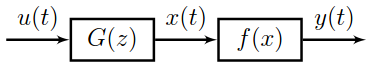
Figure 1: A discrete-time SISO Wiener model ($G$ is a linear dynamic system and $f$ is a nonlinear static system)

The recent book Giri & Bai (2010) also provides some industrial relevant examples of Wiener, Hammerstein, and Wiener-Hammerstein models, that can be handled by the Wiener-Schetzen model structure due to its parallel nature. In fact, a Wiener-Schetzen model can describe a large class of nonlinear systems arbitrarily well in mean-square sense (see Schetzen (2006) for the theory and other practical examples). If the system has fading memory, then for bounded slew-limited inputs, a uniform convergence is obtained (Boyd & Chua, 1985). In a Wiener-Schetzen model, the dynamics are described in terms of orthonormal basis functions (OBFs). The nonlinearity is described by a multivariate polynomial. Though any complete set of OBFs can be chosen, the choice is important for the convergence rate. If the pole locations of the OBFs match the poles of the underlying linear dynamic system closely, this linear dynamic system can be described accurately with only a limited number of OBFs (Heuberger et al., 2005). In the original ideas of Wiener (Wiener, 1958), Laguerre OBFs were used. Laguerre OBFs are characterized by a real-valued pole, making them suitable for describing well-damped systems with dominant first-order dynamics. For moderately damped systems with dominant second-order dynamics, using Kautz OBFs is more appropriate (da Rosa et al., 2007; Van den Hof et al., 1995). We choose generalized OBFs (GOBFs), since they can deal with multiple real and complex valued poles (Heuberger et al., 2005).

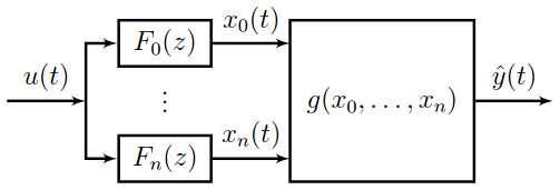
Figure 2: A Wiener-Schetzen model ($F_{0},\ldots,F_{n}$ are scalar OBFs and $g$ is a multivariate polynomial function)

This paper considers the approximation of a Wiener system with finite-order IIR (infinite impulse response) dynamics and a polynomial nonlinearity by a Wiener-Schetzen model that contains a limited number of GOBFs. The system poles are first estimated using the best linear approximation (BLA) (Pintelon & Schoukens, 2012) of the system. Next, the GOBFs are constructed using these pole estimates. The coefficients of the multivariate polynomial are determined with a linear regression. The approach can be applied to parallel Wiener systems as well. As the estimation is linear-in-the-parameters, the Wiener-Schetzen model is well suited to provide an initial guess for nonlinear optimization algorithms, and for modeling time-varying and parameter-varying systems. The analysis in this paper is a starting point to tackle these problems.

The contributions of this paper are:

• the proposal of an identification method for Wiener systems with finite-order IIR dynamics (the initial ideas were presented in Tiels & Schoukens (2011)),

• a convergence analysis for the proposed method.

The paper is organized as follows. The basic setup is described in Section 2. Section 3 presents the identification procedure and the convergence analysis. Section 4 discusses the sensitivity to output noise. The identification procedure is illustrated on two simulation examples in Section 5. Finally, the conclusions are drawn in Section 6.

2 Setup

This section first introduces some notation, and next defines the considered system class and the class of excitation signals. Afterwards, the Wiener-Schetzen model is discussed in more detail. A brief discussion of the BLA concludes this section.

2.1 Notation

This section defines the notations $\operatorname{plim}$, $O(\cdot)$, and $O_{p}(\cdot)$.

Notation 1 ($\operatorname{plim}$, (Pintelon & Schoukens, 2012)).

The sequence $x(N)$, $N=1,2,\ldots$ converges to $x$ in probability if, for every $\epsilon,\delta>0$ there exists an $N_{0}$ such that for every $N>N_{0}$ : $P(\left|x(N)-x\right|\leq\epsilon)>1-\delta$. We write

$$\begin{gathered}\operatorname{plim}_{N\rightarrow\infty}x(N)=x\\ \Leftrightarrow\forall\epsilon>0:\lim_{N\rightarrow\infty}P(\left|x(N)-x\right|\leq\epsilon)=1\end{gathered}$$

Notation 2 ($O(\cdot)$).

The notation $h_{1}$ is an $O(N^{\alpha})$ indicates that for $N$ big enough, $\lvert h_{1}(N)\rvert\leq c{N}^{\alpha}$, where $c$ is a strictly positive real number.

Notation 3 ($O_{p}(\cdot)$, (van der Vaart, 1998)).

The notation $h_{2}$ is an $O_{p}({N}^{\alpha})$ indicates that the sequence $h_{2}(N)$ is bounded in probability at the rate $N^{\alpha}$. More precisely, $h_{2}(N)=h_{3}(N)N^{\alpha}$, where $h_{3}(N)$ is a sequence that is bounded in probability.

2.2 The Wiener system

The data-generating system is assumed to be a single input single output (SISO) discrete-time Wiener system (see Fig. 1). This is the cascade of a linear time-invariant (LTI) system $G(z)$ and a static nonlinear system $f(x)$.

In this paper, $G(z)$ is restricted to be a stable, rational transfer function, and $f(x)$ to be a polynomial.

Definition 1.

The class $\mathcal{G}$ is the set of proper, finite-dimensional, rational transfer functions, that are analytic in $|z|\geq 1$ and squared integrable on the unit circle.

Assumption 1.

The LTI system $G(z)\in\mathcal{G}$.

Assumption 2.

The order of $G(z)\in\mathcal{G}$ is known.

The poles of $G(z)$ are denoted by $p_{j}$ ($j=1,\ldots,n_{p}$).

Assumption 3.

The function $f(x)$ is non-even around the operating point.

Assumption 4.

The function $f(x)$ is a polynomial of known degree $Q$:

$$f(x)=\sum_{p=0}^{Q}\gamma_{p}x^{p}\quad.$$ (1)

More general functions can be approximated arbitrarily well in mean-square sense by (1) over any finite interval.

The input $u(t)$ and the output $y(t)=f(x(t))$ are measured at time instants $t=kT_{s}$ ($k=0,\ldots,N-1$).

2.3 Random-phase multisine excitation

In this paper, random-phase multisine (Pintelon & Schoukens, 2012) excitations are considered.

Definition 2.

A signal $u(t)$ is a random-phase multisine if (Pintelon & Schoukens, 2012)

$$u(t)=\sum_{k=-N_{F}}^{N_{F}}U_{k}e^{j2\pi\frac{kf_{max}}{N_{F}}t}\quad,$$ (2)

with $U_{k}=U_{-k}^{*}=|U_{k}|e^{j\phi_{k}}$, $f_{max}=\frac{N_{F}}{NT_{s}}$ the maximum frequency of the excitation signal, $N_{F}\leq\frac{N}{2}$ the number of frequency components, and the phases $\phi_{k}$ uniformly distributed in the interval $[0,2\pi[$.

The amplitudes $|U_{k}|$ can be chosen by the user, and are normalized such that $u(t)$ has finite power as $N_{F}\rightarrow\infty$ (Pintelon & Schoukens, 2012).

Definition 3.

The class of excitation signals $\mathcal{E}$ is the set of random-phase multisines $u(t)$, having normalized amplitudes $U_{k}=\frac{1}{\sqrt{N_{F}}}\check{U}\left(\frac{kf_{max}}{N_{F}}\right)$, where $\check{U}(\frac{\omega}{2\pi})\in\mathbb{R}^{+}$ is a uniformly bounded function ($\check{U}(\frac{\omega}{2\pi})\leq M_{U}/\sqrt{2}<\infty$) with a countable number of discontinuities, and $U_{k}=0$ if $\left|k\right|>N_{F}$ or $k=0$.

Assumption 5.

The excitation signal $u(t)\in\mathcal{E}$.

For simplicity, the excitations in this paper are restricted to random-phase multisines. However, as shown in Schoukens et al. (2009), the theory applies for a much wider class of Riemann-equivalent signals. In this case, these are the extended Gaussian signals, which among others include Gaussian noise.

2.4 The Wiener-Schetzen model

The system is modeled with a Wiener-Schetzen model (Fig. 2), where we choose $F_{1}(z),\ldots,F_{n}(z)$ to be GOBFs.

In Heuberger et al. (2005), it is shown how a set of poles gives rise to a set of OBFs

$$F_{l}(z)=\frac{\sqrt{1-|\xi_{l}|^{2}}}{z-\xi_{l}}\prod_{i=1}^{l-1}\left[\frac{1-\xi_{i}^{*}z}{z-\xi_{i}}\right]\quad.$$ (3a)

If the poles $$\xi_{l}$$ result from a periodic repetition of a finite set of poles, the GOBFs are obtained, with poles

$$\xi_{j+(k-1)n_{\xi}}=\xi_{j}\qquad j=1,\ldots,n_{\xi};\,k=1,2,\ldots\quad.$$ (3b)

The GOBFs form an orthonormal basis for the set of (strictly proper) rational transfer functions in $\mathcal{G}$ (Heuberger et al., 2005). One extra basis function is introduced, namely $F_{0}(z)=1$, to enable the estimation of a feed-through term and as such also to enable the estimation of static systems (Tiels & Schoukens, 2011). This extra basis function is still orthogonal with respect to the other basis functions (see Appendix A).

The LTI system $G(z)$ can thus be represented exactly as a series expansion in terms of the basis functions $F_{l}(z)$:

$$G(z)=\sum_{l=0}^{\infty}\alpha_{l}F_{l}(z)\quad.$$ (4)

Let $\hat{G}(z,n_{rep})=\sum_{l=0}^{n}\alpha_{l}F_{l}(z)$ be a truncated series expansion, with $n=n_{rep}n_{\xi}$, and $n_{rep}$ the number of repetitions of the finite set of poles $\{\xi_{1},\ldots,\xi_{n_{\xi}}\}$. Recall that $p_{j}$ ($j=1,\ldots,n_{p}$) are the true poles of $G(z)$, and let

$$\rho=\max_{j}\prod_{k=1}^{n_{\xi}}\left|\frac{p_{j}-\xi_{k}}{1-p_{j}\xi_{k}}\right|\quad.$$ (5)

Then there exists a finite $c_{GOBF}\in\mathbb{R}$, such that for any $\eta\in\mathbb{R}$, $0\leq\rho<\eta<1$ (de Vries & Van den Hof, 1998; Heuberger et al., 1995)

$$\|G(z)-\hat{G}(z,n_{rep})\|_{\infty}\leq c_{GOBF}\frac{\eta^{n_{rep}}}{1-\eta}\quad,$$ (6)

which shows that $G(z)$ can be well approximated with a small number of GOBFs if the poles $\xi_{j}$ are close to the true poles $p_{j}$. The pole locations $p_{j}$ will be estimated by means of the BLA of the system.

2.5 The best linear approximation

The BLA of a system is defined as the linear system that approximates the system’s output best in mean-square sense (Pintelon & Schoukens, 2012). The BLA of the considered Wiener system is equal to (Schoukens et al., 1998)

$$G_{BLA}(e^{j\omega_{k}})=c_{BLA}\,G(e^{j\omega_{k}})+O({N_{F}}^{-1})\quad,$$ (7)

where the constant $c_{BLA}$ depends upon the odd nonlinearities in $f(x)$ and the power spectrum of the input signal $u(t)\in\mathcal{E}$. A similar result for Gaussian noise excitations results from Bussgang’s theorem (Bussgang, 1952).

Remark 1.

Under Assumption 3, $c_{BLA}$ is non-zero.

3 Identification procedure (no output noise)

This section formulates the identification procedure and provides a convergence analysis in the noise-free case. The influence of output noise is analyzed in Section 4.

The basic idea is that the asymptotic BLA ($N_{F}\rightarrow\infty$) has the same poles as $G(z)$ (see (7)). The poles calculated from the estimated BLA are thus excellent candidates to be used in constructing the GOBFs. Since the BLA will be estimated from a finite data set ($N_{F}$ finite), the poles calculated from the estimated BLA will differ from the true poles. Extensions of the basis functions ($n_{rep}>1$) will be used to compensate for these errors (see (6)).

The identification procedure can be summarized as:

1. Estimate the BLA and calculate its poles.

2. Use these pole estimates to construct the GOBFs.

3. Estimate the multivariate polynomial coefficients.

These steps are now formalized and the asymptotic behavior ($N_{F}\rightarrow\infty$) of the estimator is analyzed. First, the situation without disturbing noise is considered. The influence of disturbing noise is discussed in Section 4.

3.1 Identify the BLA and calculate its poles

3.1.1 Nonparametric and parametric BLA

First, a nonparametric estimate of the BLA is calculated. Since the input is periodic, the BLA is estimated as $\hat{G}_{BLA}(e^{j\omega_{k}})=\frac{Y(e^{j\omega_{k}})}{U(e^{j\omega_{k}})}$, in which $Y(e^{j\omega_{k}})$ and $U(e^{j\omega_{k}})$ are the discrete Fourier transforms (DFTs) of the output and the input. For random excitations, the classical frequency response estimates (division of cross-power and auto-power spectra) can be used (Pintelon & Schoukens, 2012), or more advanced FRF measurement techniques can be used, like the local polynomial method (Pintelon et al., 2010).

Next, a parametric model is identified using a weighted least-squares estimator (Schoukens et al., 1998)

$$\hat{\theta}(N_{F})=\operatorname*{arg\,min}_{\theta}K_{N_{F}}(\theta)\quad,$$ (8a)

where the cost function $$K_{N_{F}}(\theta)$$ is equal to

$$\frac{1}{N_{F}}\sum_{k=1}^{N_{F}}W(k)\left|\hat{G}_{BLA}(e^{j\omega_{k}})-G_{M}(e^{j\omega_{k}},\theta)\right|^{2}\quad.$$ (8b)

Here, $$W(k)\in\mathbb{R}^{+} \theta G_{M}(e^{j\omega_{k}},\theta)$$ is a deterministic, -independent weighting sequence, and is a parametric transfer function model

$$\begin{gathered}G_{M}(e^{j\omega_{k}},\theta)=\frac{\sum_{l=0}^{n_{b}}b_{l}e^{-j\omega_{k}l}}{\sum_{l=0}^{n_{a}}a_{l}e^{-j\omega_{k}l}}=\frac{B_{\theta}(e^{j\omega_{k}})}{A_{\theta}(e^{j\omega_{k}})}\quad,\\ \theta=\begin{bmatrix}a_{0}&\cdots&a_{n_{a}}&b_{0}&\cdots&b_{n_{b}}\end{bmatrix}^{T}\quad,\end{gathered}$$ (8c)

with the constraint $$\|\theta\|_{2}=1 n_{a}=n_{p}$$ to obtain a unique parameterization. Under Assumption 2, we put .

3.1.2 Pole estimates

Eventually, the poles $\hat{p}_{j}$ ($j=1,\ldots,n_{p}$) of the parametric model $G_{M}(e^{j\omega_{k}},\hat{\theta})$ are calculated. Before we derive a bound on $\Delta p_{j}:=\hat{p}_{j}-p_{j}$ in Lemma 1, a regularity condition on the parameter set $\theta$ is needed.

Assumption 6.

The parameter set $\theta$ is identifiable if the system is excited by $u(t)\in\mathcal{E}$.

The existence of a uniformly bounded convergent Volterra series (Schetzen, 2006; Schoukens et al., 1998) is needed as well (see Appendix B for more details).

Assumption 7.

There exists a uniformly bounded Volterra series whose output converges in least-squares sense to the true system output for $u(t)\in\mathcal{E}$.

Lemma 1.

Consider a discrete-time Wiener system, with an LTI system $G(z)$ and a static nonlinear system $f(x)$. Let $p_{j}$ ($j=1,\ldots,n_{p}$) be the poles of $G(z)$ and $\hat{p}_{j}$ be the pole estimates, obtained using the weighted least-squares estimator (8). Then under Assumptions 1 – 3, and 5 – 7, $\Delta p_{j}:=\hat{p}_{j}-p_{j}$ is an $O_{p}({N_{F}}^{-1/2})$.

Let $\tilde{\theta}$ be the “true” model parameters, such that

$$\begin{aligned} G_{M}(e^{j\omega_{k}},\tilde{\theta})&=c_{BLA}G(e^{j\omega_{k}})\\ &=\frac{B_{\tilde{\theta}}(e^{j\omega_{k}})}{A_{\tilde{\theta}}(e^{j\omega_{k}})}\end{aligned}\quad\forall\omega_{k}\quad,$$ (9)

with $A_{\tilde{\theta}}$ and $B_{\tilde{\theta}}$ polynomials of degree $n_{p}$. The roots of $A_{\tilde{\theta}}(e^{j\omega_{k}})$ are equal to the true poles $p_{j}$ ($j=1,\ldots,n_{p}$). If these poles are all distinct, the first-order Taylor expansion of $A_{\tilde{\theta}}(e^{j\omega_{k}})$ results in (Guillaume et al., 1989)

$$\Delta p_{j}\approx-\sum_{l=0}^{n_{a}}\frac{{p_{j}}^{l}}{A_{\tilde{\theta}}^{{}^{\prime}}(p_{j})}\Delta a_{l}\quad,$$ (10a)

where $$A_{\tilde{\theta}}^{{}^{\prime}}(p_{j})\neq 0 \Delta a_{l}$$, and where follows from

$$\hat{\theta}-\tilde{\theta}=\begin{bmatrix}\Delta a_{0}&\cdots&\Delta a_{n_{a}}&\Delta b_{0}&\cdots&\Delta b_{n_{b}}\end{bmatrix}^{T}\quad.$$ (10b)

Under Assumptions 5 – 7, it is shown in Schoukens et al. (1998) that $\operatorname{plim}_{N_{F}\rightarrow\infty}\left(\hat{\theta}(N_{F})-\tilde{\theta}\right)=0$. For the considered output disturbances (no noise in this section, filtered white noise in Section 4), the least-squares estimator (8) is a MLE (Pintelon et al., 1994). From the properties of the MLE, it follows that (Pintelon & Schoukens, 2012)

$$\hat{\theta}=\tilde{\theta}+O_{p}({N_{F}}^{-1/2})\quad.$$ (11)

Then from (10) and (11), it follows that

$$\Delta p_{j}=O_{p}({N_{F}}^{-1/2})\quad.$$ (12)

This concludes the proof of Lemma 1. ∎ Lemma 1 shows that good pole estimates are obtained.

Remark 2.

Though no external noise is considered in this section, the probability limits in this paper are w.r.t. the random phase realizations of the excitation signal.

3.2 Construct the GOBFs

Next, the GOBFs are constructed with these pole estimates (see (3), with $\xi_{j}=\hat{p}_{j}$), and the intermediate signals $x_{l}(t)=F_{l}(z)u(t)$ ($l=0,\ldots,n$) (see Fig. 2) are calculated. The following lemma shows that the true intermediate signal $x(t)$ can be approximated arbitrarily well by a linear combination of the calculated signals $x_{l}(t)$.

Lemma 2.

Consider the situation of Lemma 1. Let $F_{0}(z)=1$, and let $F_{l}(z)$ ($l=1,2,\ldots$) be GOBFs, constructed from the finite set of poles $\{\hat{p}_{1},\ldots,\hat{p}_{n_{p}}\}$. Let $x(t)=G(z)u(t)$ and $x_{l}(t)=F_{l}(z)u(t)$. Let $G(z)=\sum_{l=0}^{\infty}\alpha_{l}F_{l}(z)$, and denote $n=n_{rep}n_{p}$. Then under Assumptions 1 – 3, and 5 – 7, $\Delta x(t):=x(t)-\sum_{l=0}^{n}\alpha_{l}x_{l}(t)$ is an $O_{p}({N_{F}}^{-n_{rep}/2})$.

From (5) and (12), it follows that $\rho$ is an $O_{p}({N_{F}}^{-1/2})$. It then follows from (6) that $G(z)-\sum_{l=0}^{n}\alpha_{l}F_{l}(z)=O_{p}({N_{F}}^{-n_{rep}/2})$, and thus $\Delta x(t)$ is an $O_{p}({N_{F}}^{-n_{rep}/2})$. ∎

3.3 Estimate the multivariate polynomial coefficients

Finally, the coefficients of the multivariate polynomial $g(x_{0},\ldots,x_{n})$ are estimated. Let

$$y_{\beta}=\beta_{DC}+\sum_{p=1}^{Q}\left(\sum_{i_{1}=0}^{n}\sum_{i_{2}=i_{1}}^{n}\cdots\sum_{i_{p}=i_{p-1}}^{n}\beta_{i_{1},\ldots,i_{p}}x_{i_{1}}\cdots x_{i_{p}}\right)$$ (13a)

be the output of $$g(x_{0},\ldots,x_{n})$$, where the coefficients of the polynomial are chosen to be

$$\beta=\begin{bmatrix}\beta_{DC}&\beta_{0}&\cdots&\beta_{i_{1},\ldots,i_{p}}&\cdots&\beta_{n,\ldots,n}\end{bmatrix}^{T}\quad.$$ (13b)

They are estimated using linear least-squares regression:

$$\hat{\beta}=\operatorname*{arg\,min}_{\beta}\|y_{\beta}-y\|_{2}=\operatorname*{arg\,min}_{\beta}\|\Psi\beta-y\|_{2}\quad,$$ (14a)

where the regression matrix $$\Psi$$ is equal to

$$\Psi=\begin{bmatrix}1&\cdots&1\\ x_{0}(0)&\cdots&x_{0}(N-1)\\ \vdots&\ddots&\vdots\\ x_{i_{1}}(0)\cdots x_{i_{p}}(0)&\cdots&x_{i_{1}}(N-1)\cdots x_{i_{p}}(N-1)\\ \vdots&\ddots&\vdots\\ {x_{n}}^{Q}(0)&\cdots&{x_{n}}^{Q}(N-1)\end{bmatrix}^{T}$$ (14b)

We will now show that the estimated output $\hat{y}(t):=y_{\hat{\beta}}$ converges in probability to $y(t)$ as $N_{F}\rightarrow\infty$.

Theorem 1.

Consider the situation of Lemma 2. Let $y(t)=f(x(t))$ and $\hat{y}(t)=y_{\hat{\beta}}(t)$, where the coefficients $\hat{\beta}$ are obtained from the least-squares regression (14). Then under Assumptions 1 – 7, $\hat{y}(t)-y(t)$ is an $O_{p}({N_{F}}^{-n_{rep}/2})$.

The exact output

$$y(t) =\sum_{p=0}^{Q}\gamma_{p}x^{p}(t)$$ (15)

$$=\sum_{p=0}^{Q}\gamma_{p}\left(\sum_{l=0}^{n}\alpha_{l}x_{l}(t)+\Delta x(t)\right)^{p}$$

$$=\left[\sum_{p=0}^{Q}\gamma_{p}\left(\sum_{l=0}^{n}\alpha_{l}x_{l}(t)\right)^{p}\right]+\Delta y$$

$$=\begin{aligned} &\tilde{\beta}_{DC}\\ &+\sum_{p=1}^{Q}\left(\sum_{i_{1}=0}^{n}\sum_{i_{2}=i_{1}}^{n}\cdots\sum_{i_{p}=i_{p-1}}^{n}\tilde{\beta}_{i_{1},\ldots,i_{p}}x_{i_{1}}\cdots x_{i_{p}}\right)\\ &+\Delta y\end{aligned}$$

$$=y_{\tilde{\beta}}+\Delta y$$

where $y_{\tilde{\beta}}$ is the output of a multivariate polynomial $g(x_{0},\ldots,x_{n})$, in which the coefficients $\tilde{\beta}$ follow from the true coefficients $\gamma_{p}$ of $f(x)$ and the true coefficients $\alpha_{l}$ of the series expansion of $G(z)$. The truncation of this series expansion is taken into account by the term $\Delta y$, which just as $\Delta x$ is an $O_{p}({N_{F}}^{-n_{rep}/2})$.

Note that the coefficients $\tilde{\beta}$ can be obtained as the minimizers of the artificial least-squares problem

$$\tilde{\beta}=\operatorname*{arg\,min}_{\beta}\|\Psi\beta-y_{\tilde{\beta}}\|_{2}\quad.$$ (16)

The estimated coefficients are equal to

$$\begin{aligned} \hat{\beta}&=(\Psi^{T}\Psi)^{-1}\Psi^{T}y\\ &=(\Psi^{T}\Psi)^{-1}\Psi^{T}(y_{\tilde{\beta}}+\Delta y)\\ &=\tilde{\beta}+(\Psi^{T}\Psi)^{-1}\Psi^{T}\Delta y\end{aligned}\quad.$$ (17)

We now show that $(\Psi^{T}\Psi)^{-1}\Psi^{T}\Delta y$ is an $O_{p}({N_{F}}^{-n_{rep}/2})$.

Each element in $\Psi$ is an $O({N_{F}}^{0})$, due to the normalization of the excitation signal (see Assumption 5). Consequently, each element in the matrix $\Psi^{T}\Psi$ is the sum of $N$ terms that are an $O({N_{F}}^{0})$, so $\Psi^{T}\Psi$ is an $O(N)$. The elements in the matrix $(\Psi^{T}\Psi)^{-1}$ are thus an $O(N^{-1})$.

Each element in the vector $\Delta y$ is an $O_{p}({N_{F}}^{-n_{rep}/2})$. Consequently, each element in the vector $\Psi^{T}\Delta y$ is the sum of $N$ terms that are the product of an $O({N_{F}}^{0})$ and an $O_{p}({N_{F}}^{-n_{rep}/2})$. The elements in the vector $\Psi^{T}\Delta y$ are thus an $O(N)O_{p}({N_{F}}^{-n_{rep}/2})$.

As a consequence, $\hat{\beta}=\tilde{\beta}+O_{p}({N_{F}}^{-n_{rep}/2})$. And thus

$$\hat{y}(t)-y(t)=\Psi(\hat{\beta}-\tilde{\beta})-\Delta y=O_{p}({N_{F}}^{-n_{rep}/2})\quad.$$ (18)

This concludes the proof of Theorem 1. ∎ Theorem 1 shows that the estimated output converges in probability to the exact output with only a finite number of basis functions. The convergence rate increases if $n_{rep}$ is increased.

Remark 3.

The multivariate polynomial $g(x_{0},\ldots,x_{n})$ is implemented in terms of Hermite polynomials (Schetzen, 2006) to improve the numerical conditioning of the least-squares estimation in (14) (Tiels & Schoukens, 2011). As this has no consequences for the result in Theorem 1, ordinary polynomials are used throughout the paper to keep the notation simple.

4 Noise analysis

In this section, the sensitivity of the identification procedure to output noise is discussed. Noise on the intermediate signal $x(t)$ is not considered here. In general, this would result in biased estimates of the nonlinearity. More involved estimators, e.g. the MLE, are needed to obtain an unbiased estimate (Hagenblad et al., 2008; Wills et al., 2013).

In the case of filtered white output noise $v(t)=H(q)e(t)$, with $e(t)$ a sequence of independent random variables, independent of $u(t)$, with zero mean and variance $\lambda$, and with $H(q)$ a stable monic filter, the exact output $y(t)=y_{\tilde{\beta}}(t)+\Delta y(t)+v(t)$. The estimated coefficients are then equal to (cfr. (17))

$$\hat{\beta}=\tilde{\beta}+(\Psi^{T}\Psi)^{-1}\Psi^{T}\Delta y+(\Psi^{T}\Psi)^{-1}\Psi^{T}v\quad.$$ (19)

The columns of $\Psi$ are filtered versions of the known input signal $u(t)$, which was assumed independent of $v(t)$. It is thus clear that the noise $v(t)$ is uncorrelated with the columns of $\Psi$. Consequently, each element in the vector $\Psi^{T}v$ is the sum of $N$ uncorrelated terms that are the product of an $O({N_{F}}^{0})$ and an $O(N^{0})$. The elements in the vector $\Psi^{T}v$ are thus an $O(N^{1/2})$, As a consequence, $(\Psi^{T}\Psi)^{-1}\Psi^{T}v=O(N^{-1/2})$.

The error on the estimated output due to the noise is thus independent of the number of repetitions $n_{rep}$. Increasing $n_{rep}$ allows to tune the model error such that it disappears in the noise floor.

5 Illustration

In this section, the approach is illustrated on two simulation examples. The first one considers the noise-free case, and illustrates the convergence rate predicted by Theorem 1. The second one compares the proposed method to the so-called approximative prediction error method (PEM) (Hagenblad et al., 2008), as implemented in the MATLAB system identification toolbox (Ljung, 2013).

5.1 Example 1: noise-free case

Consider a SISO discrete-time Wiener system with

$$G(z)=\frac{1+3z^{-1}+3z^{-2}+z^{-3}}{1-2.1z^{-1}+1.9z^{-2}-0.7z^{-3}}\quad,$$ (20)

and

$$f(x)=x+0.8x^{2}+0.7x^{3}\quad.$$ (21)

The system is excited with a random-phase multisine (see (2)) with $f_{max}=f_{s}/6$ and $f_{s}$ the sampling frequency; $N_{F}=170,341,682,1365,2730,5461,10922$; and the amplitudes $|U_{k}|$ chosen equal to each other and such that the rms value of $u(t)$ is equal to $1$. The system is identified using the identification procedure described in Section 3. No weighting is used to obtain a parametric estimate of the BLA, i.e. $W(k)=1$ in (8b). A random-phase multisine with $N_{F}=10922$ is used for the validation. Fifty Monte Carlo simulations are performed, with each time a different realization of the random phases of the excitation signals.

The results in Fig. 3 show that the convergence rate of $(\hat{y}(t)-y(t))$ agrees with what is predicted by Theorem 1. The convergence rate increases with an increasing number of repetitions of the basis functions. These results generalize to parallel Wiener systems as well.

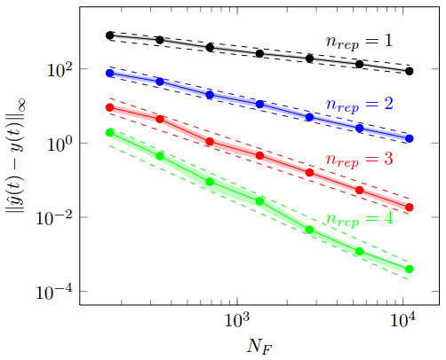
Figure 3: Average of $\left\|\hat{y}(t)-y(t)\right\|_{\infty}$ along the $50$ Monte Carlo simulations (full line) and its one standard deviation confidence interval (filled zone). The predicted convergence rate is indicated by the dashed lines, which are an $O({N_{F}}^{-n_{rep}/2})$.

5.2 Example 2: noisy case with saturation nonlinearity

The second example is inspired by the second example in Hagenblad et al. (2008). It is a discrete-time SISO Wiener system with a saturation nonlinearity. The system is given by

$$\begin{aligned} &x(t)+0.3x(t-1)-0.3x(t-2)\\ &\quad=u(t)-0.3u(t-1)+0.3u(t-2)\\ &f(x(t))=\begin{cases}c_{1}&\text{for }x(t)\leq c_{1}\\ x(t)&\text{for }c_{1}<x(t)\leq c_{2}\\ c_{2}&\text{for }c_{2}<x(t)\end{cases}\\ &y(t)=f\left(x(t)\right)+e(t)\end{aligned}\quad,$$ (22)

where the input $u$ and the output noise $e$ are Gaussian, with zero mean, and with variances $\lambda_{u}=1$ and $\lambda_{e}=0.01$ respectively. The coefficients $c_{1}$ and $c_{2}$ are equal to $-0.4$ and $0.2$, respectively. Compared to the example in Hagenblad et al. (2008), no process noise was added to $x(t)$ since the GOBF approach cannot deal with process noise. Moreover, the output noise variance was lowered from $\lambda_{e}=0.1$ to $\lambda_{e}=0.01$ as the large output noise would otherwise dominate so much that no sensible conclusions could be made.

One thousand Monte Carlo simulations are performed, with each time an estimation and a validation data set of $N=1000$ data points each. In case of the approximative PEM method (Hagenblad et al., 2008), the true model structure is assumed to be known, and the true system belongs to the considered model set. In case of the proposed GOBF approach, the order of the linear dynamics is assumed to be known. A model with $n_{rep}=0$ and one with $n_{rep}=1$ is estimated. The local polynomial method (Pintelon et al., 2010) is used to estimate the BLA. The nonlinearity is approximated via a multivariate polynomial of degree $3$, in order to capture both even and odd nonlinearities. Note that in this case, the true system is not in the model set.

The results in Fig. 4 show that the approximative PEM method performs significantly better than the GOBF approach. Note that the approximative PEM method used full prior knowledge of the model structure, while no prior knowledge on the nonlinearity was used in the GOBF approach. Still, it is able to find a decent approximation. A better approximation can be obtained by representing the nonlinearity with another basis function expansion that is more appropriate to the nonlinearity at hand. This, however, is out of the scope of this paper. Finally, for a single-branch Wiener system, the shape of the output nonlinearity can be determined as follows. Motivated by Lemma 2 and (7), an estimate of the coefficients $\alpha$ can be obtained as

$$\hat{\alpha}=\operatorname*{arg\,min}_{\alpha}\left\lvert y(t)-\sum_{l=0}^{n}\alpha_{l}x_{l}(t)\right\rvert^{2}\quad.$$ (23)

The signal $\hat{x}(t)=\sum_{l=0}^{n}\alpha_{l}x_{l}(t)$ is then, up to an unknown scale factor $c_{BLA}$, approximately equal to $x(t)$. The shape of the nonlinear function $f$ can then be determined from a scatter plot of $\hat{x}(t)$ and $y(t)$ (see Fig. 5).

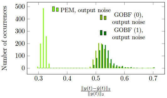
Figure 4: Distribution of $\frac{\left\|y(t)-\hat{y}(t)\right\|_{2}}{\left\|y(t)\right\|_{2}}$ on the validation data sets for the $1000$ Monte Carlo simulations. PEM indicates the results for the approximative prediction error method, while GOBF (0) and GOBF (1) indicate the results for the proposed GOBF approach with $n_{rep}=0$ and $n_{rep}=1$.

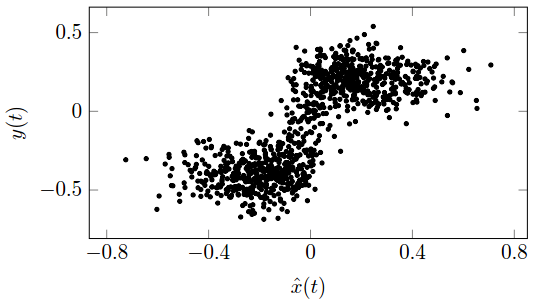
Figure 5: The scatter plot of $\hat{x}(t)$ and $y(t)$ reveals the shape of the saturation nonlinearity (GOBF approach with $n_{rep}=0$, last Monte Carlo simulation).

To make a fair comparison, the example is modified such that the system is in the model class for both of the considered approaches. The nonlinearity in (22) is changed to a third-degree polynomial that best approximates the saturation nonlinearity on all the estimation data sets. The approximative PEM method now estimates a third-degree polynomial nonlinearity. In this case, the GOBF approaches have a similar performance as the approximative PEM approach (see Fig. 6). Finally, in order to determine the number of repetitions $n_{rep}$, one can easily estimate several models for an increasing $n_{rep}$, and compare the simulation errors on a validation data set. Once the simulation error increases, the variance error outweighs the model error, and one should select less repetitions. Here, the normalized rms error for $n_{rep}=0$ is lower than the normalized rms error for $n_{rep}=1$ in $850$ out of the $1000$ cases. In the remaining $150$ cases, one would select a model with $n_{rep}\geq 1$.

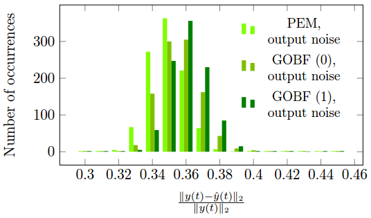
Figure 6: Distribution of $\frac{\left\|y(t)-\hat{y}(t)\right\|_{2}}{\left\|y(t)\right\|_{2}}$ on the validation data sets for the $1000$ Monte Carlo simulations (polynomial nonlinearity).

6 Conclusion

An identification procedure for SISO Wiener systems with finite-order IIR dynamics and a polynomial nonlinearity was formulated and its asymptotic behavior was analyzed in an output-error framework. It is shown that the estimated output converges in probability to the true system output. Fast convergence rates can be obtained.

The identification procedure is mainly linear in the parameters. The proposed identification procedure is thus well suited to provide an initial guess for nonlinear optimization algorithms. The approach can be applied to parallel Wiener systems as well.

This work was supported by the ERC advanced grant SNLSID, under contract 320378.

Appendix A Orthonormal basis

The orthogonality of $F_{0}(z)$ with respect to the set $\{F_{l}(z)\}$ ($l=1,2,\ldots$) can be shown either by working out the inner products $\langle F_{l}(z),F_{0}(z)\rangle$ (see below) or by choosing a pole structure $\{0,\xi_{1},\xi_{2},\ldots\}$ in the shifted basis functions $F_{l}^{S}(z):=zF_{l}(z)$.

Consider the basis functions $F_{l}^{B}(z)$, given by $F_{j+(k-1)n_{\xi}}^{B}(z)=\frac{1}{(z-\xi_{j})^{k}}$ for $j=1,\ldots,n_{\xi}$ and $k=1,2,\ldots$. We now prove that they are orthogonal to $F_{0}(z)=1$, by showing that the inner product

$$\langle F_{j+(k-1)n_{\xi}}^{B}(z),F_{0}(z)\rangle$$ (24)

$$\qquad=\frac{1}{2\pi i}\oint_{\mathbb{T}}F_{j+(k-1)n_{\xi}}^{B}(z)F_{0}^{*}\left(\frac{1}{z^{*}}\right)\frac{\mathrm{d}z}{z}\quad,$$

is equal to zero. $\mathbb{T}$ denotes the unit circle.

1. $\xi_{j}\neq 0$
   

   $$\langle F_{j+(k-1)n_{\xi}}^{B}(z),F_{0}(z)\rangle$$ (25)

   $$\qquad=\frac{1}{2\pi i}\oint_{\mathbb{T}}\frac{1}{z(z-\xi_{j})^{k}}\mathrm{d}z$$

   $$\qquad=\frac{1}{(k-1)!}\lim_{z\rightarrow\xi_{j}}\frac{\mathrm{d}^{k-1}}{\mathrm{d}z^{k-1}}\left(\frac{1}{z}\right)+\lim_{z\rightarrow 0}\frac{1}{(z-\xi_{j})^{k}}$$

   $$\qquad=\frac{1}{(k-1)!}(-1)^{k-1}(k-1)!\,\xi_{j}^{-k}+(-1)^{k}\xi_{j}^{-k}$$

   $$\qquad=\xi_{j}^{-k}\left((-1)^{k-1}+(-1)^{k}\right)$$

   $$\qquad=0$$

2. $\xi_{j}=0$
   

   $$\langle F_{j+(k-1)n_{\xi}}^{B}(z),F_{0}(z)\rangle =\frac{1}{2\pi i}\oint_{\mathbb{T}}\frac{1}{z^{k+1}}\mathrm{d}z$$ (26)

   $$=\frac{1}{k!}\lim_{z\rightarrow 0}\left.\left.\frac{\mathrm{d}^{k}}{\mathrm{d}z^{k}}\right(1\right)$$

   $$=0$$

The OBFs $F_{l}(z)$ are linear combinations of the basis functions $F_{l}^{B}(z)$ (Heuberger et al., 2005) and are thus orthogonal to $F_{0}(z)=1$. Since the norm of $F_{0}(z)$ is equal to one, the set $\{F_{l}(z)\}$ ($l=0,1,\ldots$) is a set of OBFs. ∎

Appendix B Volterra series

A Volterra series generalizes the impulse response of an LTI system to a nonlinear time-invariant system via multidimensional impulse responses. The input-output relation of a Volterra series is split in different contributions of increasing degree of nonlinearity (Schetzen, 2006)

$$y(t)=\sum_{p=1}^{\infty}y_{p}(t)\quad,$$ (27a)

with

$$y_{p}(t)=\int_{-\infty}^{+\infty}\cdots\int_{-\infty}^{+\infty}h_{p}(\tau_{1},\ldots,\tau_{p})\\ u(t-\tau_{1})\cdots u(t-\tau_{p})\mathrm{d}\tau_{1}\cdots\mathrm{d}\tau_{p}\quad,$$ (27b)

where $h_{p}$ is the Volterra kernel of degree $p$.

For periodic excitations, the output Fourier coefficient $Y_{p}(k)$ at frequency $\frac{kf_{max}}{N_{F}}$ is (Chua & Ng, 1979)

$$Y_{p}(k)=\sum_{k_{1}=-N_{F}}^{N_{F}}\sum_{k_{2}=-N_{F}}^{N_{F}}\cdots\sum_{k_{p-1}=-N_{F}}^{N_{F}}\\ H_{p}(L_{k},k_{1},k_{2},\ldots,k_{p-1})\\ U(k_{1})U(k_{2})\cdots U(k_{p-1})U(L_{k})\quad,$$ (28)

with $L_{k}=k-\sum_{i=1}^{p-1}k_{i}$. Here, $H_{p}$ is the symmetrized frequency domain representation of the Volterra kernel of degree $p$. The Volterra series is uniformly bounded if (Schoukens et al., 1998)

$$\sum_{p=1}^{\infty}M_{H_{p}}{M_{U}}^{p}\leq C_{1}<\infty\quad,$$ (29)

with $M_{H_{p}}=\max\left|H_{p}\right|$, and $M_{U}$ as in Definition 3.

References

- Billings & Fakhouri (1982) Billings, S. A., & Fakhouri, S. Y. (1982). Identification of systems containing linear dynamic and static nonlinear elements. Automatica, 18, 15–26.
- Bloemen et al. (2001) Bloemen, H. H. J., Chou, C. T., van den Boom, T. J. J., Verdult, V., Verhaegen, M., & Backx, T. C. (2001). Wiener model identification and predictive control for dual composition control of a distillation column. Journal of Process Control, 11, 601–620.
- Boyd & Chua (1985) Boyd, S., & Chua, L. O. (1985). Fading memory and the problem of approximating nonlinear operators with Volterra series. IEEE Transactions on Circuits and Systems, 32, 1150–1161.
- Bussgang (1952) Bussgang, J. J. (1952). Crosscorrelation functions of amplitude-distorted Gaussian signals. Technical Report 216. MIT research laboratory of electronics.
- Chua & Ng (1979) Chua, L. O., & Ng, C.-Y. (1979). Frequency domain analysis of nonlinear systems: General theory. IEE Journal on Electronic Circuits and Systems, 3, 165–185.
- Giri & Bai (2010) Giri, F., & Bai, E.-W. (Eds.) (2010). Block-oriented Nonlinear System Identification. (1st ed.). Springer.
- Giri et al. (2013) Giri, F., Rochdi, Y., Radouane, A., Brouri, A., & Chaoui, F.-Z. (2013). Frequency identification of nonparametric Wiener systems containing backlash nonlinearities. Automatica, 49, 124–137.
- Greblicki (1994) Greblicki, W. (1994). Nonparametric identification of Wiener systems by orthogonal series. IEEE Transactions on Automatic Control, 39, 2077–2086.
- Guillaume et al. (1989) Guillaume, P., Schoukens, J., & Pintelon, R. (1989). Sensitivity of roots to errors in the coefficient of polynomials obtained by frequency-domain estimation methods. IEEE Transactions on Instrumentation and Measurement, 38, 1050–1056.
- Hagenblad et al. (2008) Hagenblad, A., Ljung, L., & Wills, A. (2008). Maximum likelihood identification of Wiener models. Automatica, 44, 2697–2705.
- Heuberger et al. (1995) Heuberger, P. S. C., Van den Hof, P. M. J., & Bosgra, O. H. (1995). A generalized orthonormal basis for linear dynamical systems. IEEE Transactions on Automatic Control, 40, 451–465.
- Heuberger et al. (2005) Heuberger, P. S. C., Van den Hof, P. M. J., & Wahlberg, B. (Eds.) (2005). Modelling and Identification with Rational Orthogonal Basis Functions. London: Springer.
- Hunter & Korenberg (1986) Hunter, I. W., & Korenberg, M. J. (1986). The identification of nonlinear biological systems: Wiener and Hammerstein cascade models. Biological Cybernetics, 55, 135–144.
- Kalafatis et al. (1995) Kalafatis, A., Arifin, N., Wang, L., & Cluett, W. R. (1995). A new approach to the identification of pH processes based on the Wiener model. Chemical Engineering Science, 50, 3693–3701.
- Ljung (2013) Ljung, L. (2013). System Identification Toolbox - User’s Guide (8th ed.).
- Pelckmans (2011) Pelckmans, K. (2011). MINLIP for the identification of monotone Wiener systems. Automatica, 47, 2298–2305.
- Pintelon et al. (1994) Pintelon, R., Guillaume, P., Rolain, Y., Schoukens, J., & Van hamme, H. (1994). Parametric identification of transfer functions in the frequency domain – a survey. IEEE Transactions on Automatic Control, 39, 2245–2260.
- Pintelon & Schoukens (2012) Pintelon, R., & Schoukens, J. (2012). System Identification: A Frequency Domain Approach. (2nd ed.). Wiley-IEEE Press.
- Pintelon et al. (2010) Pintelon, R., Schoukens, J., Vandersteen, G., & Barbé, K. (2010). Estimation of nonparametric noise and FRF models for multivariable systems-part I: Theory. Mechanical Systems and Signal Processing, 24, 573–595.
- da Rosa et al. (2007) da Rosa, A., Campello, R. J. G. B., & Amaral, W. C. (2007). Choice of free parameters in expansions of discrete-time Volterra models using Kautz functions. Automatica, 43, 1084–1091.
- Schetzen (2006) Schetzen, M. (2006). The Volterra & Wiener Theories of Nonlinear Systems. Malabar, Florida: Krieger Publishing Company.
- Schoukens et al. (1998) Schoukens, J., Dobrowiecki, T., & Pintelon, R. (1998). Parametric and nonparametric identification of linear systems in the presence of nonlinear distortions - a frequency domain approach. IEEE Transactions on Automatic Control, 43, 176–190.
- Schoukens et al. (2009) Schoukens, J., Lataire, J., Pintelon, R., Vandersteen, G., & Dobrowiecki, T. (2009). Robustness issues of the best linear approximation of a nonlinear system. IEEE Transactions on Instrumentation and Measurement, 58, 1737–1745.
- Schoukens & Rolain (2012) Schoukens, M., & Rolain, Y. (2012). Parametric identification of parallel Wiener systems. IEEE Transactions on Instrumentation and Measurement, 61, 2825–2832.
- Tiels & Schoukens (2011) Tiels, K., & Schoukens, J. (2011). Identifying a Wiener system using a variant of the Wiener G-Functionals. In IEEE Conference on Decision and Control and European Control Conference (CDC-ECC11), Orlando, FL, USA.
- van der Vaart (1998) van der Vaart, A. W. (1998). Asymptotic Statistics. Cambridge University Press.
- Van den Hof et al. (1995) Van den Hof, P. M. J., Heuberger, P. S. C., & Bokor, J. (1995). System identification with generalized orthonormal basis functions. Automatica, 31, 1821–1834.
- de Vries & Van den Hof (1998) de Vries, D. K., & Van den Hof, P. M. J. (1998). Frequency domain identification with generalized orthonormal basis functions. IEEE Transactions on Automatic Control, 43, 656–669.
- Westwick & Verhaegen (1996) Westwick, D., & Verhaegen, M. (1996). Identifying MIMO Wiener systems using subspace model identification methods. Signal Processing, 52, 235–258.
- Wiener (1958) Wiener, N. (1958). Nonlinear problems in random theory. Wiley.
- Wills et al. (2013) Wills, A., Schön, T. B., Ljung, L., & Ninness, B. (2013). Identification of Hammerstein-Wiener models. Automatica, 49, 70–81.