Domain State of the ANNNI model in Two Dimensions

Abstract

We have examined the spin ordering of an axial next-nearest-neighbor Ising (ANNNI) model in two dimensions (2D) near above the antiphase ($\langle 2\rangle$ phase). We considered an $N_{R}$-replica system and calculated an overlap function $q_{m}$ between different replicas having used a cluster heat bath (CHB) Monte Carlo method. We determined transition temperature between $\langle 2\rangle$ phase and a floating incommensurate (IC) phase as $T_{C2}/J=0.89\pm 0.01$ with frustration ratio $\kappa(\equiv-J_{2}/J_{1})=0.6$. We found that the spin state at $T\gtrsim T_{C2}$ may be called as a domain state, because the spin structure is characterized by a sequentially arranged four types of domains with different $\langle 2\rangle$ structures. In the domain state, the 2D XY symmetry of the spin correlation in the IC phase weakly breaks and the diversity of the spin arrangement increases as $T\rightarrow T_{C2}$. The Binder ratio $g_{L}$ exhibits a depression at $T\sim T_{C2}$ and the quasi-periodic spin structure, which is realized in the IC phase, becomes diverse at $T\gtrsim T_{C2}$. We discussed that the domain state is stable against the thermal fluctuation which brings a two-stage development of the spin structure at low temperatures.

I Introduction

Systems with competitive interactions have been extensively studied throughout the past three decades, because they exhibit rich physical phenomena, such as commensurate-incommensurate phase transitions, Lifshitz points and multiphase points.Selke0 The axial next-nearest-neighbor Ising (ANNNI) model is among the simplest realizations of such systems. In the two-dimensional (2D) ANNNI model, ferromagnetic Ising chains are coupled by ferromagnetic nearest-neighbor and antiferromagnetic next-nearest-neighbor interchain interactions on a square lattice. The Hamiltonian is described by

$$\mathcal{H} = -\it{J}\sum_{\it{x,y}}S_{\it{x,y}}S_{\it{x+1,y}}$$ (1)

$$- \it{J_{1}}\sum_{\it{x,y}}S_{x,y}S_{x,y+1}-\it{J}_{\it{2}}\sum_{{x,y}}S_{x,y}S_{x,y+2},$$

where $S_{x,y}=\pm 1$ is an Ising spin. In this paper we consider the case with $J_{1}\;=\;J\;>0$ and $J_{2}<0$. The ground state of the model is a ferromagnetic long range order (LRO) phase for frustration coefficient $\kappa(\equiv-J_{2}/J)<1/2$ and a LRO antiphase ($\langle 2\rangle$ phase) for $\kappa>1/2$, in which the $\langle 2\rangle$ phase is described by an alternate arrangement of two up-spin and two down-spin chains in the $y$-direction. This model at finite temperatures has been studied throughout the past few decades by various methods.Selke1 ; Selke2 ; Villain ; Grynberg1 ; Saqi ; Morita It was suggested that, for $\kappa>1/2$, a floating incommensurate (IC) phase exists between the $\langle 2\rangle$ phase and the paramagnetic (PM) phase.Selke1 ; Selke2 The IC phase close to the higher transition temperature, $T_{C1}$, may be characterized by dislocationsSelke2 that play the same role of vortices in two-dimensional XY (2D XY) model,KT and the IC phase near above the lower transition temperature, $T_{C2}$, may be characterized by domain walls of three up-spin chains or three down-spin chains penetrating the $\langle 2\rangle$ phase. However, the spin ordering is yet to be clarified, because recent Monte Carlo (MC) studies predicted different spin orderings. While equilibrium MC simulations supported the above picture of the spin ordering with $T_{C2}<T_{C1}$,Sato ; Rastelli a nonequilibrium relaxation (NER) MC methodItoA ; ItoB predicted $T_{C2}\sim T_{C1}$, i.e., the absence of the IC phase.Shirahata ; Chandra In a previous paperShirakura (referred as I, hereafter), we reexamined the spin ordering of the ANNNI model with $\kappa=0.6$ near $T_{C1}$ having used both the equilibrium MC and the NER MC methods and showed that both methods give almost the same transition temperature of $T_{C1}\sim 1.16J$ and the spin ordering at $T\lesssim T_{C1}$ exhibits properties of the 2D XY model.KT

In this paper, we reexamine the spin ordering near the other transition temperature $T_{C2}$. We will propose a physical quantity appropriate for the ANNNI model, by which we can readily separate $\langle 2\rangle$ phase from the IC phase. Section II describes the investigated method and quantities of the 2D ANNNI model. Section III presents results of the equilibrium simulation. In Sec. IV, we discuss, on the basis of a domain picture, the spin structure of the model for both the temperature ranges of near below $T_{C1}(T\lesssim T_{C1})$ and near above $T_{C2}(T\gtrsim T_{C2})$. Section V is addressed on the periodic nature of the ANNNI model calculating the Fourier component of the spin arrangement. Section VI is devoted to conclusions and discussions, where we will discuss why the 2D ANNNI model undergoes a very slow relaxation at low temperatures.

II Method and Quantities

We apply a similar technique as proposed by Sato and Matsubara(SM)Sato and used in I. We consider the model with $\kappa=0.6$ on the $L_{0}\times L_{0}$ lattice with open boundaries. Quantities of interest are measured in the inner region of $L\times L$ with $L=L_{0}/2$ , i.e., $L_{0}/4+1\leq x,y\leq 3L_{0}/4$. Hereafter we attach a new lattice site name for this region, i.e., $x,y=1,2,\cdots,L$. We apply the CHB algorithmCHB1 ; CHB2 to get an equilibrium spin configuration. That is, the spin configuration of a block of $L_{0}\times l_{y}$ spins is updated using the transfer matrix method, where the transfer direction is the $x$-direction ($L_{0}$) and the width of the block $l_{y}$ is determined from the computational time costs. In the previous paper we apply the SM procedure with $l_{y}=6$. The choice of $l_{y}=6$ was appropriate in a temperature range of $T\sim T_{C1}$. However, when the temperature is lowered toward $T_{C2}$, the number of the MC sweeps needed to get the equilibrium spin configuration rapidly increases. Then we adopt a larger $l_{y}$ for a larger lattice of $L_{0}\times L_{0}$.

The difficulty of studying the phase transition of the ANNNI model is that the spin structure of the IC phase is not known a priori. Another problem to be noted is that the $\langle 2\rangle$ phase has equivalent four structures. That is, when we look at four spins at $(4l+1,4l+2,4l+3,4l+4)$ ($l=0,1,2\cdots$) chains, they have either $(++--)$, $(+--+)$, $(--++)$ or $(-++-)$. One usually investigates the squared chain magnetization $M_{2}(=\frac{1}{L}\sum_{y=1}^{L}(\frac{1}{L}\sum_{x=1}^{L}S_{x,y})^{2})$. This quantity characterizes the spin correlation along the $x$-direction. Using $M_{2}$, one can separate the IC phase from the PM phase, because in the PM phase $M_{2}$ exponentially decays with increasing $L$ and $M_{2}$ will algebraically decays in the IC phase. However, near the lower transition temperature $T_{C2}$, calculation of equilibrium value of $M_{2}$ for a larger size $L_{0}$ is hard taskSato ; Shirakura and one searches for $T_{C2}$ using different quantities.Sato ; Shirahata Moreover we can hardly investigate the 2D natue of the ANNNI model, in particular the spin correlation along the $y$-direction.

Here we consider another quantity for examining the 2D spin structure itself. We obtain the equilibrium spin configuration $\{S^{0}_{x,y}\}$ at a temperature $T$. That is, we get $\{S^{0}_{x,y}\}$ performing the MC simulation using some sequence of random numbers. Then, make the MC simulation at the same temperature $T$ using a different sequence of random numbers and get the spin configuration $\{S_{x,y}\}$. We extract the $\{S^{0}_{x,y}\}$ component of $\{S_{x,y}\}$ by calculating the spin overlap between them. To realize this procedure, we consider an $N_{R}$-replica system. The spin configurations $\{S_{x,y}^{\alpha}\}$ ($\alpha=1,2,\cdots,N_{R}$) of these replicas are generated by different sequences of random numbers. We define the $\vec{k}$-dependent maximum spin overlap function $q_{m}^{\alpha,\beta}(\vec{k})$ of the replica $\alpha$ and the replica $\beta$ as

$$q_{m}^{\alpha,\beta}(\vec{k})=q^{\alpha,\beta}(y_{0},\vec{k}),$$ (2)

where

$$y_{0}=\arg\max_{-L/2\leq y^{\prime}\leq L/2}q^{\alpha,\beta}(y^{\prime},\vec{k}),\hskip 22.76228pt$$ (3)

$$q^{\alpha,\beta}(y^{\prime},\vec{k})=\frac{1}{L^{2}}|\sum_{x=1}^{L}\sum_{y=1}^{L}S_{x,y}^{\alpha}S_{x,y+y_{0}}^{\beta}\exp(i\vec{k}\vec{r}_{x,y+y^{\prime}})|.\hskip 5.69046pt$$ (4)

In the IC phase a drift of the spin configuration inevitably occurs along the $y$-direction. We take into account the drift by a uniform shift of the spin configuration $y_{0}$. Also $q_{m}^{\alpha,\beta}(\vec{k})$ is free from the structure of the $\langle 2\rangle$ phase. The overlap function $q_{m}(\vec{k})$ of the system is the average of those overlap functions.

$$q_{m}(\vec{k})=\frac{2}{N_{R}(N_{R}-1)}\sum_{\alpha\neq\beta}q_{m}^{\alpha,\beta}(\vec{k})$$ (5)

Note that the overlap function at $\vec{k}=0$, $q_{m}(\equiv q_{m}(0))$, plays the role of the order parameter of the ANNNI model. If $q_{m}$ decys algebraicly with increasing $N$, it reveals that the system is in the critical phase, i.e., the IC phase, while $q_{m}$ remains non-zero constant, it reveals that the system is in the LRO phase, i.e., the $\langle 2\rangle$ phase. In contrast, $q_{m}(\vec{k})$ for $\vec{k}\neq 0$ will be used to obtain the correlation length of the spin structure.

III Results

We investigate the equilibrium properties of the ANNNI model by the overlap function $q_{m}$. We focus our effort in the temperature range of $T\leq T_{C1}(\sim 1.16J)$. We perform the CHB simulation of the ANNNI model on lattices with $L_{0}=24\sim 128$. We make two simulations: a gradual cooling simulation and a gradual heating simulation. In the gradual cooling (heating) simulation, we start with a PM ($\langle 2\rangle$) spin configuration at a high (low) temperature and perform the simulation described below, then the temperature is lowered (raised) by some fixed interval $\Delta T$ and perform the same simulation starting with the last spin configuration at the previous temperature, and so on. For each temperature, after $MCS_{\rm equi}$ sweeps are discarded, data of interest are measured for every 10 sweeps over $MCS_{\rm mea}$ sweeps. Data presented here are averages of those of two simulations, and errors are differences between them. Hereafter averages of data $Q$ in the inner $L\times L$ lattice are described as $\langle Q\rangle_{L}$. The parameters used in the equilibrium simulation are listed in Table 1.

Table 1: Parameters used in the CHB algorithm of the MC simulation of the $N_{R}=8$ replica system. $MCS_{\rm equi}$ and $MCS_{\rm mea}$ are the number of MC sweeps required for equilibration and measurement, respectively.

$L_{0}$	$l_{y}$	$MCS_{\rm equi}$	$MCS_{\rm mea}$
$\leq$ 48	6	4,000	12,000
64	8	10,000	30,000
96	10	20,000	60,000
128	12	40,000	80,000

III.1 Spin overlap

Figure 1 shows $\langle q_{m}\rangle_{L}$ as functions of $T$ for different $L$. At high temperatures, $\langle q_{m}\rangle_{L}$ for a larger $L$ is smaller than that for a smaller $L$. As the temperature is decreased from a high temperature, $\langle q_{m}\rangle_{L}$’s for all $L$ increase and come together at $T\sim 0.89J$. Below this temperature, the $L$-dependence of $\langle q_{m}\rangle_{L}$ is reversed. This result clearly reveals that some 2D LRO takes place at $T<0.89J$. That is, the transition temperature between the IC phase and the $\langle 2\rangle$ phase is $T_{C2}/J=0.89\pm 0.01$, because the LRO phase of the 2D ANNNI model is the $\langle 2\rangle$ phase.

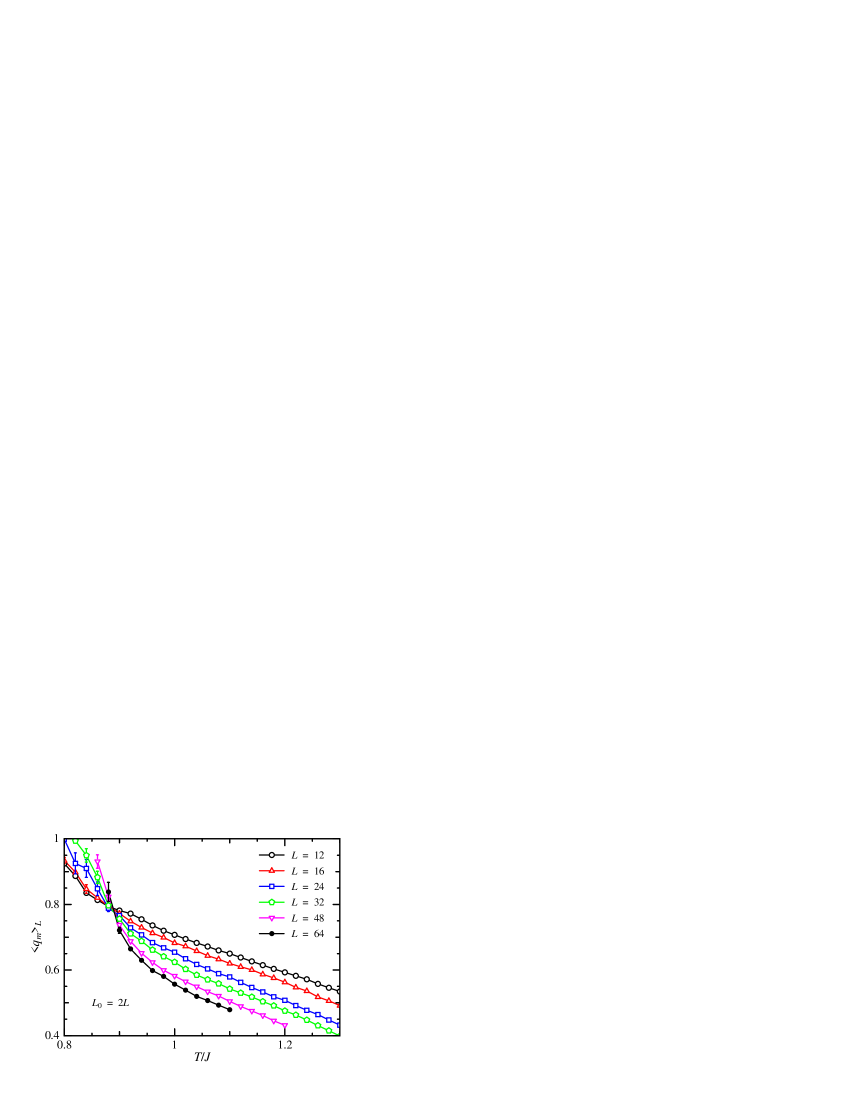
Figure 1: (color online) Temperature dependences of the spin overlap function $\langle q_{m}\rangle_{L}$ in the ANNNI model with $\kappa=0.6$, computed over the inner lattice with $L=L_{0}/2$.

III.2 Binder Ratio

Next we consider the Binder ratioBinder to examine the nature of the phase transition at $T_{C2}$. In a usual ferromagnetic(FM) model on a cubic lattice with the linear dimension $L$, the Binder ratio $g_{L}$ of the magnetization $M$ monotonically increases with decreasing temperature and reach 1 for $T\rightarrow 0$. In the PM phase, $g_{L}$ decreases with increasing $L$, while $g_{L}$ increases with $L$ in the FM phase. Then the Binder ratio is independent of $L$ at the critical temperature $T=T_{C}$. That is, the Binder ratios of different $L$’s intersect at $T=T_{C}$.

The Binder ratio $g_{L}$ of $q_{m}$ is defined as

$$g_{L}=\frac{1}{2}\left(3-\frac{\langle q_{m}^{4}\rangle_{L}}{\langle q_{m}^{2}\rangle_{L}^{2}}\right).$$ (6)

Figure 2 shows temperature dependences of $g_{L}$ for different $L$. They show unusual behaviors. For $T>T_{C2}$, $g_{L}$ increases with $L$ and seems to reach some finite value which is smaller than 1. On the other hand, for $T<T_{C2}$ $g_{L}$ rapidly increases toward 1. This result is compatible with the fact that the IC phase for $T_{C2}<T<T_{C1}$ is the KT-like phase, i.e., a critical state, and that the $\langle 2\rangle$ phase for $T<T_{C2}$ is the LRO phase. A queer point is its temperature dependence. As the temperature is decreased from a high temperature, $g_{L}$ once increases, reaches its maximum value at $T\sim 1.00J$, then decreases down to around $T_{C2}$. That is, the phase transition at $T_{C2}$ accompanies with a diversity of the spin structure.

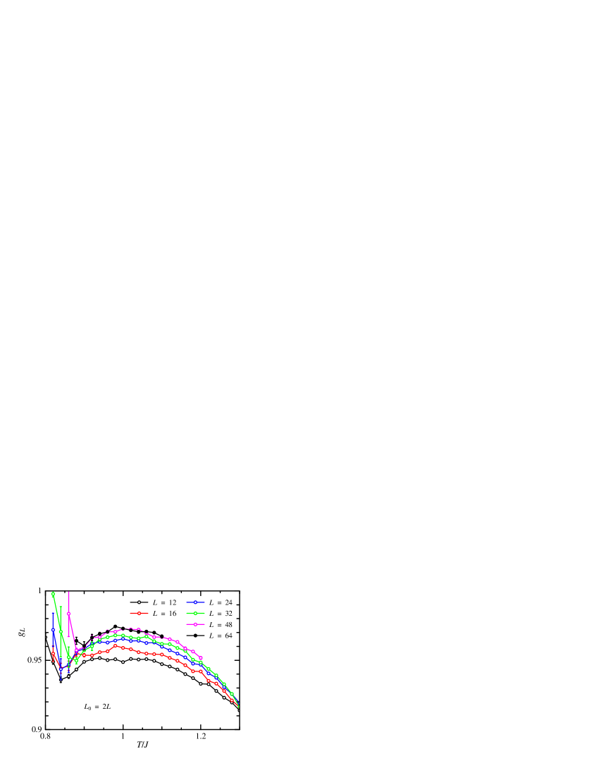
Figure 2: (color online) Temperature dependences of Binder ratio $g_{L}$ in the ANNNI model with $\kappa=0.6$ and different $L$.

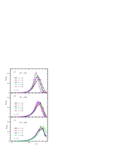
Figure 3: (color online) Distribution $P_{L}(q_{m})$ of the spin overlap $q_{m}$ in the ANNNI model with $\kappa=0.6$.

We consider the distribution $P_{L}(q_{m})$ of the order parameter $q_{m}$ to investigate the diversity of the spin structure. Attention is paid whether $P_{L}(q_{m})$ exhibits a usual single peak reminiscent of the continuous phase transition or a double peak of the first order phase transition. Figures 3(a)-(c) show $P_{L}(q_{m})$ for $T\sim T_{C2}$. They exhibit a single peak revealing that the phase transition at $T_{C2}$ is some continuous one. For $T>T_{C2}$, as $L$ increases, the peak position $q_{m}^{(p)}$ shifts to the small $q_{m}$ side and the peak height $P_{L}(q_{m}^{(p)})$ seems to saturate. These results are compatible with the $L$-dependences of $\langle q_{m}\rangle_{L}$ and $g_{L}$ shown in Figs. 1 and 2, respectively. As $T\rightarrow T_{C2}$, $P_{L}(q_{m})$ becomes broader and seems to be independent of $L$. For $T<T_{C2}$, the weight of $P_{L}(q_{m})$ at smaller $q_{m}$ diminishes and $P_{L}(1)$, which is the weight of the $\langle 2\rangle$ phase, increases. Therefore the depression of $g_{L}$ at $T\sim T_{C2}$ corresponds with a spread of $P_{L}(q_{m})$. We believe the spread attributes to a characteristic nature intrinsic to the 2D ANNNI model. We consider the $\langle 2\rangle$ phase with some $\langle 2\rangle$ structures, i.e., a single-domain state $\{S_{x,y}^{\alpha}\}$. Suppose that one domain wall penetrates in the system. Then the system is separated into two domains with different $\langle 2\rangle$ structures, i.e., a two-domain state $\{S_{x,y}^{\beta}\}$. The spin overlap function $q_{m}^{\alpha,\beta}(\vec{k})$ takes various values, depending on the location and the shape of the domain wall. Therefore the broad peak of $P_{L}(q_{m})$ at $T\gtrsim T_{C2}$ may suggest that the system is composed of domains with different $\langle 2\rangle$ structures. In this temperature range, the spin correlations along the $x$- and $y$-directions will become anisotropic.

III.3 Correlation length

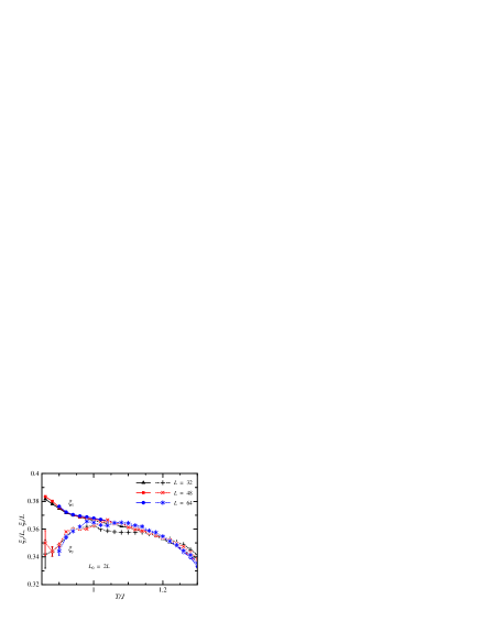
Figure 4: (color online) Temperature dependences of the correlation-length ratios $\xi_{x}/L$ (a) and $\xi_{y}/L$ (b) in the $x$ and $y$ directions, respectively, in the ANNNI model with $\kappa=0.6$.

We consider the spin correlation length $\xi_{\mu}$ along the $\mu$ direction ($\mu=x,y$) to examine the speculation mentioned above. This quantity is obtained from the spin overlap function as follows:

$$\xi_{\mu}=\frac{1}{2\sin(|\vec{k}_{\rm min}|/2)}\sqrt{\frac{\langle q_{m}^{2}\rangle_{L}}{\langle|q({\vec{k}}_{\rm min})|^{2}\rangle_{L}}-1}$$ (7)

where ${\vec{k}}_{\rm min}=(\pi/L,0)$ and ${\vec{k}}_{\rm min}=(0,\pi/L)$ in the $x$ and $y$ direction, respectively. One usually studies the ratio of the correlation length $\xi_{\mu}$ to the linear lattice size $L$, $\xi_{\mu}/L$, to determine the transition temperature $T_{C}$.Cooper Here we pay attention to the relation in the spin correlation between the $x$ and $y$ directions.

Figure 4 shows the correlation-length ratios $\xi_{x}/L$ and $\xi_{y}/L$ for different $L$ as functions of $T$. In the $x$ direction $\xi_{x}/L$ smoothly increases with decreasing temperature. On the other hand, in the $y$ direction $\xi_{y}/L$ exhibits an interesting behavior. As the temperature is decreased from a high temperature, $\xi_{y}/L$ once increases, becomes maximum at $T\sim 1.00J$, then decreases down to $T_{C2}$. We note that the temperature dependence of $\xi_{y}/L$ is quite similar to that of $g_{L}$ shown in Fig. 2. This fact indicates that the diversity of the spin structure suggested by $g_{L}$ and $P_{L}(q_{m})$ comes from the decrease of the spin correlation along the $y$ direction.

The remarkable point is that the nature of the spin correlation changes as the temperature is decreased toward $T_{C2}$. Of course, $\xi_{y}\sim\xi_{x}$ in the PM phase ($T>T_{C1}\sim 1.16J$). This relation holds near below $T_{C1}$ and remains down to $T\sim 1.0J$. That is, for $T>1.0J$ the system is almost isotropic for every direction like that of the KT phase in the 2D XY model. For $T\lesssim 1.0J$, $\xi_{x}$ and $\xi_{y}$ exhibit different temperature dependences, i.e., one increases with decreasing temperature and the other decreases. Therefore $T=1.0J$ is a temperature below which the nature of the spin correlation gradually changes from that of the KT-like state to that of another state, probably a domain state.

IV Domain Structure

Table 2: Spin arrangements of the domain element {$S_{x,y}$} $\equiv$ $(s_{x,y},s_{x,y+1},s_{x,y+2},s_{x,y+3})$ and the domain values $\tau_{x,y}(=a,b,\bar{a}$ or $\bar{b})$. Here the location of the element is distinguished by $y_{0}={\rm mod}[y,4]$.

{$S_{x,y}$}    $\setminus$   $y_{0}$				1	2	3	0
$+1$	$+1$	$-1$	$-1$	$a$	$\bar{b}$	$\bar{a}$	$b$
$+1$	$-1$	$-1$	$+1$	$b$	$a$	$\bar{b}$	$\bar{a}$
$-1$	$-1$	$+1$	$+1$	$\bar{a}$	$b$	$a$	$\bar{b}$
$-1$	$+1$	$+1$	$-1$	$\bar{b}$	$\bar{a}$	$b$	$a$

Now we examine the spin structure itself at $T\gtrsim T_{C2}$. Here we discuss it on the basis of the domain picture. For this aim, we define a domain valuable $\tau_{x,y}(=a,b,\bar{a}$ or $\bar{b})$ which describes the element of the domain. Values of $\tau_{x,y}$ are determined as follows. We consider sequential four spins ($s_{x,y},s_{x,y+1},s_{x,y+2},s_{x,y+3}$). Elements of the $\langle 2\rangle$ structure are $(+1,+1,-1,-1)$, $(+1,-1,-1,+1)$, $(-1,-1,+1,+1)$, and $(-1,+1,+1,-1)$. These elements are distinguished by the location in the lattice. Since the $\langle 2\rangle$ phase has the translational symmetry of $y\rightarrow y+4l$ $(l=1,2,\cdots)$, if the spin arrangement of $(s_{x,y+4l},s_{x,y+4l+1},s_{x,y+4l+2},s_{x,y+4l+3})$ is the same as that of $(s_{x,y},s_{x,y+1},s_{x,y+2},s_{x,y+3})$, $\tau_{x,y+4l}=\tau_{x,y}$. The spin configurations and domain values are listed in Table 2. Hereafter we describe the domain composed of $d(=a,b,\bar{a}$ or $\bar{b})$ element as $D(=A,B,\bar{A}$ or $\bar{B})$ domain, respectively, and the domain wall between the $D_{1}$ and $D_{2}$ domains as $W_{D_{1}-D_{2}}$, where $D_{1},D_{2}=A,B,\bar{A},\bar{B}$. When the D domain covers the whole lattice, we call the state the D-type $\langle 2\rangle$ phase. We readily find an interesting property of the arrangement of neighboring two domains. If the domain wall is composed of three up-spin or down-spin chains, when we watch the domain with increasing the chain site $y$, the $A$ follows the $B$, the $B$ the $\bar{A}$, the $\bar{A}$ the $\bar{B}$, and the $\bar{B}$ the $A$. That is, the domains will appear sequentially as $A\rightarrow\bar{B}\rightarrow\bar{A}\rightarrow B\rightarrow A\rightarrow\bar{B}\cdots$. An example of this is as follows.

$$\begin{array}[]{c|cccccccccccc}y&1&2&3&4&5&6&7&8&9&10&11&12\\ \hline\cr y_{0}&1&2&3&0&1&2&3&0&1&2&3&0\\ \hline\cr S_{x,y}&+1&+1&-1&-1&+1&+1&+1&-1&-1&+1&+1&-1\\ \hline\cr\tau_{x,y}&a&a&a&-&-&\bar{b}&\bar{b}&\bar{b}&\bar{b}&\bar{b}&-&-\\ \end{array}$$

$$\begin{array}[]{cccccccccccccc}13&14&15&16&17&18&19&20&21&22&23&24&25\\ \hline\cr 1&2&3&0&1&2&3&0&1&2&3&0&1\\ \hline\cr-1&-1&+1&+1&-1&-1&+1&+1&+1&-1&-1&+1&+1\\ \hline\cr\bar{a}&\bar{a}&\bar{a}&\bar{a}&\bar{a}&-&-&b&b&b&\cdot&\cdot&\cdot\\ \end{array}$$

Figures 5(a) and (b) shows the snapshots of the domain structures at $T\lesssim T_{C1}$ and at $T\gtrsim T_{C2}$, respectively. For $T\lesssim T_{C1}$, the system is composed of small domains which are separated by tangled domain walls. On the other hand, for $T\gtrsim T_{C2}$, the system is composed of several large domains each of which runs across the lattice. That is, the difference in the domain structure between the two temperature ranges are the size of the domains. For either case, four types of the domains appear in order as speculated above. We calculate the average domain width $W_{L}$ for different sizes $L$ of the lattice and extrapolate it to $L\rightarrow\infty$. Figure 6 shows $W_{L}$ as functions of $T$ together with its extrapolation. As the temperature is decreased from a high temperature, $W_{L}$ first increases slowly down to $T\sim 1.00J$, and then $W_{L}$ increases rapidly and its extrapolation seems to diverge as $T\rightarrow T_{C2}$.

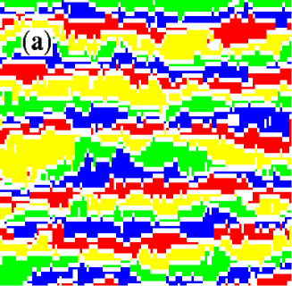
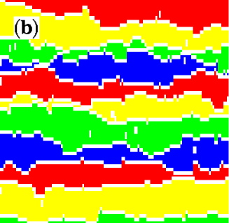
Figure 5: (color online) Snapshots of the domain structure at (a) $T=1.1J$ and (b) $T=0.92J$ in the ANNNI model with $\kappa=0.6$ on the $128\times 128$ lattice. The domain elements $a$, $b$, $\bar{a}$, and $\bar{b}$ are described by red, blue, green, and yellow, respectively, and the domain wall element by white.

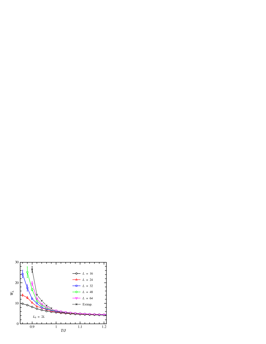
Figure 6: (color online) Temperature dependences of the average domain width $W_{L}$ of the lattice with $L$ in the ANNNI model with $\kappa=0.6$. The extrapolation to $L\rightarrow\infty$ is made using $W_{L}=W_{\infty}+A/L$ assumption.

V Fourier Component $S(k)$

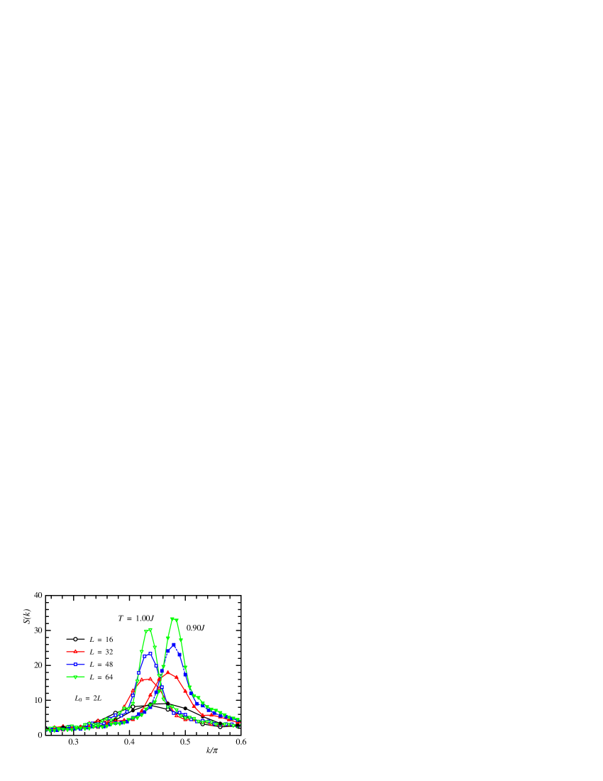
Figure 7: (color online) The Fourier components of the spin structure $S(k)$ for two temperatures well-above (open symbols) and near-above (solid symbols) $T_{C2}$.

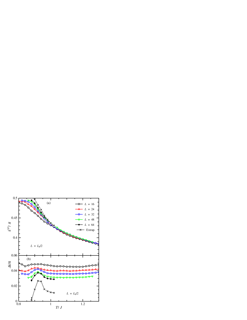
Figure 8: (color online) Temperature dependences of $k^{(p)}$ and $\Delta k$ of the lattice with $L$ in the ANNNI model with $\kappa=0.6$. The extrapolations to $L\rightarrow\infty$ for $k^{(p)}$ and $\Delta k$ are made using $k^{(p)}_{L}=k^{(p)}_{\infty}+A/L$ and $\Delta k_{L}=\Delta k_{\infty}+B/\sqrt{L}$ assumptions, respectively.

In an experimental point of view, the Fourier component of the spin arrangement is interesting. The Fourier component $S(k)$ along the $y$ direction is given by

$$S(k)=|\sum_{y=1}^{L}m(y)\exp(iky)|,$$ (8)

where $m(y)(=\sum_{x=1}^{L}S_{x,y}/L)$ is the averaged magnetization of the $y$-th chain. This quantity gives the periodicity of the spin arrangement in the $y$ direction. The period $n$ of the spin arrangement is given by $n=2\pi/k$ and the $\langle 2\rangle$ phase corresponds to $k=\pi/2$. Figure 7 shows $S(k)$ at two temperatures of well-above and near-above $T_{C2}$ for different size $L$. For either temperature, $S(k)$ exhibits a single rather broad peak which grows with increasing $L$. The result suggests that the system has a quasi-periodic spin arrangement characterized by the peak position $k^{(p)}$ and its deviation $\Delta k$. Note that the number of the periodic spin arrangements describing $S(k)$ is roughly given by $n_{p}\sim\Delta k/(\pi/L)=(\Delta k/\pi)L$. Thus $\Delta k$ gives the diversity of the spin structure. Here we estimate the peak $k^{(p)}$ and its deviation $\Delta k$ from

$$k^{(p)} = \sum_{k=\pi/L}^{\pi}k\tilde{S}(k)/\sum_{k=\pi/L}^{\pi}\tilde{S}(k)$$ (9)

$$(\Delta k)^{2} = \sum_{k=\pi/L}^{\pi}(k-k^{(p)})^{2}\tilde{S}(k)/\sum_{k=\pi/L}^{\pi}\tilde{S}(k).$$ (10)

where $\tilde{S}(k)=S(k)-\sum_{k=\pi/L}^{\pi}S(k)/{L}$. We calculate $k^{(p)}$ and $\Delta k$ for different $L$ and extrapolate them to $L\rightarrow\infty$. Figures 8(a) and (b) show $k^{(p)}$ and $\Delta k$ for different $L$ as functions of $T$, respectively, together with their extrapolated values. As the temperature is decreased from a high temperature, $k^{(p)}$ increases toward $k^{(p)}=\pi/2$ at $T_{C2}$. On the other hand, $\Delta k$ changes a little above $T_{C2}$ and the extrapolation value has a finite value, suggesting that some quasi-periodic spin structure occurs above $T_{C2}$. A notable thing is that $\Delta k$ has a mound near above $T_{C2}$. Again we see that the diversity of the spin structure along the $y$-direction is enhanced at $T\gtrsim T_{C2}$. For $T<T_{C2}$, $\Delta k$ diminihes revealing that the spin structure in the $\langle 2\rangle$ phase is periodic with period four.

VI Discussion and conclusions

We have examined the spin ordering near the lower transition temperature $T_{C2}$ of the 2D ANNNI model with $\kappa=0.6$ having used a CHB Monte Carlo method. We considered an $N_{R}$-replica system and calculated an overlap function $q_{m}$ between different replicas. We determined $T_{C2}/J=0.89\pm 0.01$ and examined the nature of the spin structure at $T\gtrsim T_{C2}$ by the use of different quantities. The results were summarized in Fig. 9. In the floating IC phase, the nature of the spin correlation for $T\gtrsim T_{C2}$ are considerably different from that for $T\lesssim T_{C1}$. For $T\gtrsim T_{C2}$, the system is characterized by large domains each of which run across the lattice. Therefore we may call the spin structure for $T\gtrsim T_{C2}$ a domain state.

Figure 9: (color online) The spin ordering of the 2D ANNNI model with $\kappa=0.6$

In the domain state in Fig. 9, the 2D XY symmetry of the spin correlation breaks, i.e., the spin correlation length in the axial direction $\xi_{y}$ decreases with lowering temperature in contrast with a monotonous increase of that in the chain direction $\xi_{x}$. In consequence, the diversity of the spin arrangement increases as $T\rightarrow T_{C2}$ and the Binder ratio $g_{L}$ exhibit a depression at $T\sim T_{C2}$. Also the quasi-periodic spin structure, which is realized in the IC phase, becomes diverse at $T\gtrsim T_{C2}$.

Here we consider properties of the domain state. We first note that an isolated domain is unstable, because it readily collapses with thermal noise. On the other hand, the domain state occurring at $T\gtrsim T_{C2}$ is sequentially arranged four types of domains: $A\rightarrow\bar{B}\rightarrow\bar{A}\rightarrow B\rightarrow A\rightarrow\bar{B}\cdots$. This structure is stable against the thermal fluctuation. We consider the $A$-type $\langle 2\rangle$ phase with three domains of $\bar{B},\bar{A}$, and $B$. Suppose that the $\bar{B}$ domain collapses. Then domain arrangement becomes as $A\rightarrow\bar{A}\rightarrow B\rightarrow A$ and an unfavorable domain wall of $W_{A-\bar{A}}$ appears. This domain structure is unstable and as soon as the $\bar{B}$ collapses, another $\bar{B}$ arises between the $A$ and the $\bar{A}$ domains, because further collapse of the $\bar{A}$ also yields unfavorable domain wall $W_{A-B}$. Therefore the collapse of three domains of $\bar{B},\bar{A}$, and $B$ will occur concurrently. This is a very rare event especially at low temperatures, because the domain size becomes larger and larger as the temperature is decreased toward $T_{C2}$. The reverse is also true. That is, the concurrence of three domains in the $\langle 2\rangle$ phase is also very rare event. These properties explain a well-known phenomenon of the 2D ANNNI model, i.e., a huge number of the MC sweep is necessary to get an equilibrium spin configuration.

Also development of the spin structure exhibits an interesting property in this temperature range. Figure 10 shows the development of the maximum spin overlap $q_{m}(t)$ starting with paramagnetic spin configuration for various temperatures. Here we adopt a single-spin-flip heat-bath MC algorithm and $t$ being the number of the MC sweep. For a temperature well-above $T_{C2}$, $q_{m}(t)$ monotonously increases toward $q_{m}(\infty)$, which is estimated in the equilibrium CHB MC simulation. On the other hand, for temperatures $T\sim T_{C2}$, $q_{m}(t)$ exhibits two-stage development. In the first stage, it increases algebraically with $t$ and reach a value of $\bar{q_{m}}\sim 0.5$ at $\bar{t}\sim 10^{4}$, which are almost independent of the temperature (even for well-below $T_{C2}$). In the second stage, $q_{m}(t)$ slowly increases with $t$ until $q_{m}(t)$ reaches its equilibrium value $q_{m}(\infty)$. Again we see $q_{m}(t)$ are almost independent of the temperature within this time scale. We find that this two-stage development of $q_{m}(t)$ comes from the domain structure of the model. Figure 11 shows the $t$ dependence of $S(k)$ at $T\sim T_{C2}$. As $t$ increases from $t=0$, the peak of $S(k)$ develops and becomes of a single-peaked at $t\sim 10^{4}$. Above this time, the peak position $\bar{k}$ increases very slowly toward to $k_{p}$ of the equilibrium result with clarifying its shape. That is, the first stage of the development of the spin structure is the creation of some quasi-periodic spin arrangement, and in the second stage the period of the periodic structure is gradually changes to fit its equilibrium one. The later stage is the collapse of different domains which is very slow as discussed above.

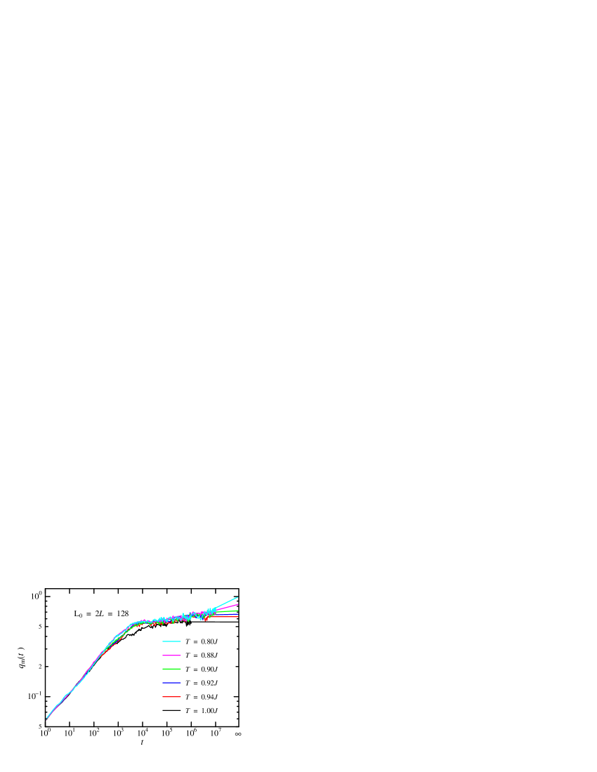
Figure 10: (color online) The MC sweep $t$ dependence of the maximum spin overlap $q_{m}(t)$ starting with paramagnetic spin configuration in the ANNNI model with $\kappa=0.6$. The last points are ones estimated by the equilibrium CHB simulation.

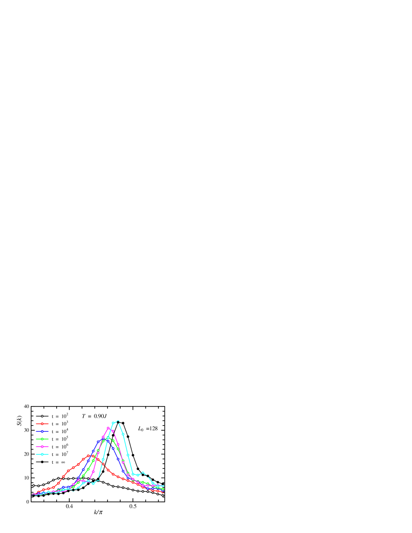
Figure 11: (color online) The MC sweep $t$ dependence of the Fourier component $S(k)$ of the spin structure starting with paramagnetic spin configuration in the ANNNI model with $\kappa=0.6$. $S(k)$ for $t=\infty$ is one estimated by the equilibrium CHB simulation.

References

References

- (1) For example see, e.g., W. Selke, in PHASE TRANSITIONS AND CRITICAL PHENOMENA, ed. C. Domb and J. L. Lebowitz (Academic Press, 1992), Vol. 15, p. 1; and references therein.
- (2) W. Selke and M.E. Fisher, Z. Physik B 40, 71 (1980).
- (3) W. Selke, K. Binder, and W. Kinzel, Surf. Sci. 125, 74 (1983).
- (4) J. Villain and P. Bak, J. Phys.(Paris) 42, 657 (1981).
- (5) M. D. Grynberg and H. Ceva, Phys. Rev. B 36, 7091 (1987).
- (6) M. A. S. Saqi and D. S. McKenzie, J. Phys. A: Math. Gen. 20 471 (1987).
- (7) Y. Murai, K. Tanaka and T. Morita, Physica A 217, 214 (1995).
- (8) J. M. Kosterlitz and D. J. Thouless, J. Phys. C6, 1181 (1973).
- (9) A. Sato and F. Matsubara, Phys. Rev. B 60, 10316 (1999).
- (10) E. Rastelli, S. Regina and A. Tassi, Phys. Rev. B 81, 094425 (2010).
- (11) N. Ito, Physica A 192, 604 (1993).
- (12) N. Ito and Y. Ozeki, Int. J. Mod. Phys. C 10, 1495 (1999).
- (13) T. Shirahata and T. Nakamura, Phys. Rev. B 65, 024402 (2001).
- (14) A. K. Chandra and S. Dasgupta, J. Phys. A: Math. Theor. 40 6251 (2007).
- (15) T. Shirakura, F. Matsubara, and N. Suzuki, Phys. Rev. B 90, 144410 (2014).
- (16) O. Koseki and F. Matsubara, J. Phys. Soc. Jpn. 66, 322 (1997).
- (17) F. Matsubara, A. Sato, O. Koseki, and T. Shirakura, Phys. Rev. Lett. 78, 3237 (1997).
- (18) K. Binder, Z. Phys. B: Condens. Matter 43, 119 (1981).
- (19) F. Cooper, B. Freedman, and D. Preston, Nucl. Phys. B 210, 210 (1989).