Optimized effective potential method and application to static RPA correlation

Abstract

The optimized effective potential (OEP) method is a promising technique for calculating the ground state properties of a system within the density functional theory. However, it is not widely used as its computational cost is rather high and, also, some ambiguity remains in the theoretical framework. In order to overcome these problems, we first introduced a method that accelerates the OEP scheme in a static RPA-level correlation functional. Second, the Krieger-Li-Iafrate (KLI) approximation is exploited to solve the OEP equation. Although seemingly too crude, this approximation did not reduce the accuracy of the description of the magnetic transition metals (Fe, Co, and Ni) examined here, the magnetic properties of which are rather sensitive to correlation effects. Finally, we reformulated the OEP method to render it applicable to the direct RPA correlation functional and other, more precise, functionals. Emphasis is placed on the following three points of the discussion: i) Level-crossing at the Fermi surface is taken into account; ii) eigenvalue variations in a Kohn-Sham functional are correctly treated; and iii) the resultant OEP equation is different from those reported to date.

Keywords: Density functional theory, exchange-correlation functional, optimized effective potential, random phase approximation.

1 Introduction

In the Kohn-Sham scheme of density functional theory, the exchange-correlation energy functional plays a key role in determining the accuracy of a calculation because the majority of the many-body effects are incorporated in the functional. The local density approximation (LDA) has been the most widely-used approximation of this functional, as a result of its simplicity, small computational cost, and its unexpectedly accurate description of matter. However, there is a growing need for methods with both higher accuracy and tolerable computational cost for practical use. The optimized effective potential (OEP) method[1, 2] is a promising approach that offers a means of including more accurate exchange-correlation functionals in such calculations. Its theoretical flexibility comes from the fact that the OEP is a general method used to minimize the energy functionals that are explicitly expressed in terms of the Kohn-Sham orbitals. Of the possible functionals, a formalism that takes account of the random-phase-approximation (RPA)-level correlation is considered to be an important step as regards reasonable descriptions of solid systems. Kotani[3] included such RPA-level correlation with a static approximation and obtained reasonable results for realistic systems. These results were sufficiently encouraging, however, this type of self-consistent calculation has not become widely-used. This can be attributed to its highly time-consuming procedures, which are used during every iteration step in order to obtain a self-consistent result.

Two of the procedures are rate-determining. One, which is common to all the OEP calculations, is a procedure that solves the OEP equation. As regards this stage, several authors have already proposed techniques[4, 5, 6, 7] and approximations[8, 9, 10, 11, 12, 13, 14, 15] that accelerate the process. The other rate-determining procedure is the calculation of the variation of the static RPA (sRPA) correlation energy, which has attracted only minor attention to date. However, this is an unavoidable issue if one considers practical use of the sRPA functional. For the former procedure, an approximation of the OEP equation proposed by Krieger, Li, and Iafrate[8, 9] (KLI) will be used in the present paper. It appears to be a crude approximation, and it was also shown by Krieger et al. that this formalism can be regarded as only a lowest level approximation in a systematic improvement scheme[16]. However, it has been reported that the KLI approximation does not contradict the numerical predictions for some isolated systems[8, 9, 17]. We also reported[18] that it does not negatively affect descriptions of some extended systems within the exact-exchange (EXX) functional level, provided a slight modification to the KLI scheme is employed. Then, a natural question is whether the modified KLI approximation is still feasible within the OEP+sRPA scheme. In order to answer this query, errors from additional procedures used to calculate the correlation effects must be suppressed. For example, the summation of unoccupied orbitals in the procedure for calculating the variation of the sRPA functional seems a considerable obstacle to retaining the necessary accuracy; this also renders the procedure time-consuming. In order to achieve both acceleration and precision, we have devised a method that avoids such a summation without loss of accuracy. We will show that, with this method, the modified KLI approximation does not reduce the accuracy of the descriptions of the magnetic transition metals studied here, namely, Fe, Ni, and Co.

Reformulation of the OEP method is also discussed in the present paper. In our opinion, the standard derivations of the OEP equation are incomplete. This is reflected in an unphysical degree of freedom entering the equation obtained by Sharp and Horton[1] and by Talman and Shadwick[2] (SHTS). In our discussion, we will incorporate the dependency of the Kohn-Sham energy-functional on eigenvalues and also consider level-crossing at the Fermi surface. In addition, we will discuss how these factors have been neglected in the standard derivations. Concerning the level-crossing effects, we have already presented some of this discussion in our previous paper[18], with a view to providing a complementary equation to the SHTS equation. A result in the present paper justifies the use of this complementary equation. As for treatment of the eigenvalues, this has been ignored for a long time. However, variations with respect to the eigenvalues cannot be ignored in these calculations, because they are linked to a variation of density via an effective potential in the Kohn-Sham equation, with

$$\left[-\nabla^{2}+V_{{\rm eff},\sigma}(\bm{r})\right]\psi_{i\sigma}(\bm{r})=\epsilon_{i\sigma}\psi_{i\sigma}(\bm{r}),$$ (1)

where the ground-state density determines the corresponding effective potential, $V_{\rm eff}$. The Kohn-Sham orbital, $\psi_{i\sigma}$, and its eigenvalue, $\epsilon_{i\sigma}$, are determined by $V_{\rm eff}$. With consideration of the eigenvalue-dependency, we will derive a correction term to the SHTS equation in the following section. It is also shown that this correction term is fortunately canceled in the static RPA functional, but this cancellation does not occur in general.

This paper will show the derivation of OEP-EXX+sRPA technique, reformulate the OEP method, and provide sample calculations and results. The structure of the paper is as follows: Section 2 is devoted to our formalism. In this section, for convenience, reformulation of the OEP precedes specific topics concerning the sRPA correlation. Details and results of the calculations obtained using our OEP-EXX+sRPA technique are shown and discussed in section 3. In the last section, section 4, we present a summary and conclusions.

2 Theory

2.1 Reformulation of optimized effective potentials

In the Kohn-Sham scheme, the ground-state spin-density, $n_{\sigma}^{0}$, is determined through minimization of the Kohn-Sham energy functional, $E_{\rm KS}$, such that

$$\left.\frac{\delta E_{\rm KS}[n_{\uparrow},n_{\downarrow}]}{\delta n_{\sigma}({\bm{r}})}\right|_{n_{\sigma}=n_{\sigma}^{0}}=0,$$ (2)

where the number of electrons and the spin-density, $n_{-\sigma}$, of the opposite spin direction is fixed. In the standard derivations of the OEP equation, the variation of the density, $n_{\sigma}$, is decomposed into the variations of the effective potential, $V_{{\rm eff},\sigma}$, the Kohn-Sham orbitals, $\{\psi_{i\sigma}\}_{i}$, and their conjugates, with

$$\frac{\delta}{\delta n_{\sigma}(\bm{r})}=\sum_{i}\int d{\bm{r}}^{\prime}\,d{\bm{r}}^{\prime\prime}\left(\frac{\delta V_{{\rm eff},\sigma}({\bm{r}}^{\prime})}{\delta n_{\sigma}({\bm{r}})}\frac{\delta\psi_{i\sigma}({\bm{r}}^{\prime\prime})}{\delta V_{{\rm eff},\sigma}({\bm{r}}^{\prime})}\frac{\delta}{\delta\psi_{i\sigma}({\bm{r}}^{\prime\prime})}+\rm{c.c.}\right).$$ (3)

However, it is often forgotten that the variation of the effective potential in equation (3) must be restricted in an unusual way in order to keep $n_{-\sigma}$ fixed. Specifically, variation of the potential ($\delta V_{{\rm eff},\sigma}$) that perturbs an eigenvalue, $\epsilon_{i\sigma}$, away from the Fermi sea must be excluded if an unoccupied opposite-spin state becomes occupied. This is in order to conserve the number of electrons in the perturbed system. Otherwise, a change in $n_{-\sigma}$ is permitted. Neglecting this restriction on $\delta V_{{\rm eff},\sigma}$ leads to an incorrect value for $\frac{\delta V_{{\rm eff},\sigma}}{\delta n_{\sigma}}$ in equation (3), and an extra degree of freedom is introduced to the resultant potential. This explains how the well-known unphysical insensitivity to the transform

$$V_{{\rm eff},\sigma}\rightarrow V_{{\rm eff},\sigma}+C_{\sigma}$$ (4)

is introduced in the SHTS equation, where $C_{\sigma}$ is an arbitrary real number.

There appears to be no easy means of removing such a forbidden $\delta V_{{\rm eff},\sigma}$ in $\frac{\delta V_{{\rm eff},\sigma}}{\delta n_{\sigma}}.$ However, this difficulty can be avoided by taking $V_{{\rm eff},\uparrow}$ and $V_{{\rm eff},\downarrow}$ as variables independent from each other in the minimization of $E_{\rm KS}$, and by allowing $V_{{\rm eff},\sigma}$ to change $n_{-\sigma}$. However, in this alternative strategy, the implicit expectation that $E_{\rm KS}$ is a functional of Kohn-Sham orbitals only, as described in equation (3), is no longer acceptable, because $V_{{\rm eff},\sigma}$ can change $n_{-\sigma}$ by only perturbing eigenvalues of spin-direction $\sigma$. Let us take the LDA for example. The LDA can be treated in the standard OEP derivation with the relation

$$n_{\sigma}(\bm{r})[\{\psi^{*}_{i\sigma},\psi_{i\sigma}\}_{i}]=\sum_{i=1}^{N_{\sigma}}\psi^{*}_{i\sigma}(\bm{r})\psi_{i\sigma}(\bm{r}),$$ (5)

where $N_{\sigma}$ denotes the number of occupied Kohn-Sham orbitals for spin $\sigma$. Here, the Kohn-Sham functional should be expressed explicitly in terms of orbitals as

$$E^{\rm LDA}_{\rm KS}[\{\psi^{*}_{i\sigma},\psi_{i\sigma}\}]=J_{\rm KS}[\{\psi^{*}_{i\sigma},\psi_{i\sigma}\}]+E^{\rm LDA}_{\rm xc}[\{n_{\sigma}[\{\psi^{*}_{i\sigma},\psi_{i\sigma}\}_{i}]\}],$$ (6)

with

$$J_{\rm KS}=\sum_{\sigma}\sum_{i=1}^{N_{\sigma}}\int d{\bm{r}}\,\psi^{*}_{i\sigma}(\bm{r})[-\nabla^{2}+V_{\rm ext}(\bm{r})]\psi_{i\sigma}(\bm{r})+E_{\rm Hartree}[\{\psi^{*}_{i\sigma},\psi_{i\sigma}\}],$$ (7)

and

$$E_{\rm Hartree}=\sum_{\sigma,\sigma^{\prime}}\sum_{i=1}^{N_{\sigma}}\sum_{j=1}^{N_{\sigma^{\prime}}}\int d{\bm{r}}\,d{\bm{r}}^{\prime}\,\frac{\psi^{*}_{i\sigma}(\bm{r})\psi_{i\sigma}(\bm{r})\psi^{*}_{j\sigma^{\prime}}({\bm{r}}^{\prime})\psi_{j\sigma^{\prime}}({\bm{r}}^{\prime})}{\left|{\bm{r}}-{\bm{r}}^{\prime}\right|}.$$ (8)

In a standard treatment, $N_{\sigma}$ must be fixed during the variation because $N=N_{\uparrow}+N_{\downarrow}$ must be conserved and $n_{-\sigma}$ must be constant. In contrast, we must treat the implicit eigenvalue-dependence of $N_{\sigma}$ in our alternative strategy because we are allowing $V_{{\rm eff},\sigma}$ to change $N_{-\sigma}$ through eigenvalues at the Fermi level.

However, one should also note that a set of eigenvalues, $\{\epsilon_{i\sigma}\}$, is not a functional of the spin-density only because there exists a freedom in the choice of reference energy. On the other hand, the exact $E_{\rm KS}$ is a functional of the spin-density only. Therefore, it is natural to introduce another variable that can refer to the origin of the energy, so that it can cancel unwanted dependences on the reference energy. Let $\mu$ denote such a variable, one of the possible definitions of which is as follows. For a given $\{n_{\sigma}\}$, the independent variable $\mu$ determines $\{\epsilon_{i\sigma}\}$ so that $\mu$ becomes a minimum real number that causes the relation

$$N=\lim_{\delta\mu\rightarrow 0^{+}}\sum_{i,\sigma}\theta(\mu+\delta\mu-\epsilon_{i\sigma})\ ,$$ (9)

to hold, where $\theta$ is the step function and the summation is taken over all the orbitals regardless of their occupancy. In order for $\{\epsilon_{i\sigma}\}$ to be determined uniquely, even for cases involving semiconductors or insulators, the “minimum real” feature is required. In most cases, one can neglect the existence of $\delta\mu$ by simply substituting zero in its place and defining $\theta(0)=1$. We use this condition for simplicity hereafter. Note that the dependency of each $\epsilon_{i\sigma}$ on the energy-reference is canceled by subtraction of $\mu$ in equation (9). Let us return to the LDA example with the definition of $\mu$ given above. The spin-density, $n_{\sigma}$, can be expressed naturally using $\mu$ as

$$n_{\sigma}({\bm{r}})=\sum_{i}\theta(\mu-\epsilon_{i\sigma})\,\psi^{*}_{i\sigma}({\bm{r}})\psi_{i\sigma}({\bm{r}}),$$ (10)

and is now re-expressed as a functional of $\{\psi^{*}_{i\sigma},\psi_{i\sigma}\}$, $\{\epsilon_{i\sigma}\}$, and $\mu$.

Equation (6) in its entirety can also be given naturally as

$$E^{\rm LDA}_{\rm KS}\left[\{\psi^{*}_{i\sigma},\psi_{i\sigma}\},\{\epsilon_{i\sigma}\},\mu\right]$$

$$=J_{\rm KS}\left[\{\psi^{*}_{i\sigma},\psi_{i\sigma}\},\{\epsilon_{i\sigma}\},\mu\right]+E^{\rm LDA}_{\rm xc}\left[\left\{n_{\sigma}\left[\{\psi^{*}_{i\sigma},\psi_{i\sigma}\}_{i},\{\epsilon_{i\sigma}\}_{i},\mu\right]\right\}_{\sigma}\right],$$ (11)

with

$$J_{{\rm KS}}=\sum_{i,\sigma}\theta(\mu-\epsilon_{i\sigma})\,\psi^{*}_{i\sigma}({\bm{r}})\left[-\nabla^{2}+V_{\rm ext}({\bm{r}})\right]\psi_{i\sigma}({\bm{r}})+E_{\rm Hartree}\left[\{\psi^{*}_{i\sigma},\psi_{i\sigma}\},\{\epsilon_{i\sigma}\},\mu\right],$$ (12)

and

$$E_{\rm Hartree}=\sum_{i,\sigma}\theta(\mu-\epsilon_{i\sigma})\sum_{j,\sigma^{\prime}}\theta(\mu-\epsilon_{j\sigma^{\prime}})\int d{\bm{r}}\,d{\bm{r}}^{\prime}\,\frac{\psi^{*}_{i\sigma}({\bm{r}})\psi_{i\sigma}({\bm{r}})\psi^{*}_{j\sigma^{\prime}}({\bm{r}}^{\prime})\psi_{j\sigma^{\prime}}({\bm{r}}^{\prime})}{\left|{\bm{r}}-{\bm{r}}^{\prime}\right|},$$ (13)

where $V_{\rm ext}$ is a fixed external potential.

As shown in the above example, we must manage a functional that depends at least on $\{\psi^{*}_{i\sigma},\psi_{i\sigma}\}$, $\{\epsilon_{i\sigma}\}$, and $\mu$ in general. Therefore, in the following, we consider a generalized Kohn-Sham functional in the form, $E_{\rm KS}\left[\{\psi^{*}_{i\sigma},\psi_{i\sigma}\},\{\epsilon_{i\sigma}\},\mu\right].$ Equations for $V_{{\rm eff},\uparrow}$, $V_{{\rm eff},\downarrow}$, and $\mu$ are obtained by minimizing $E_{\rm KS}$ with the number of electrons fixed and the “minimum real” requirement for $\mu$. Each of the variables, $V_{{\rm eff},\uparrow}$, $V_{{\rm eff},\downarrow}$, and $\mu$, can be treated as being independent from each other through use of the Lagrange multiplier method. Note that the generalized $E_{\rm KS}$ includes functionals that depend on the choice of reference energy as well as those that do not. The properties of the Kohn-Sham functionals that are invariant under alteration of the reference energy will be addressed later.

We now discuss the minimization of $E_{\rm KS}$, again adopting the definition of $\mu$ given in (9). The “minimum real” requirement for $\mu$ in equation (9) is expressed in an analytic form, such that

$$P=\lim_{\delta\mu\rightarrow 0^{+}}\prod_{i\sigma}\theta(\mu+\delta\mu-\epsilon_{i\sigma})\times(\mu+\delta\mu-\epsilon_{i\sigma})=0,\\$$ (14)

which is sufficient because a constraint on equation (9) is also required for electron-number conservation. The Kohn-Sham functional can be written as

$$E_{\rm KS}\left[\{\psi^{*}_{i\sigma},\psi_{i\sigma}\},\{\epsilon_{i\sigma}\},\mu\right]=J_{\rm KS}\left[\{\psi^{*}_{i\sigma},\psi_{i\sigma}\},\{\epsilon_{i\sigma}\},\mu\right]+E_{\rm xc}\left[\{\psi^{*}_{i\sigma},\psi_{i\sigma}\},\{\epsilon_{i\sigma}\},\mu\right],$$ (15)

with $J_{\rm KS}$ as defined in equation (12). The chain rule for the variation of $V_{{\rm eff},\sigma}({\bm{r}})$ is

$$\frac{\delta}{\delta V_{{\rm eff},\sigma}({\bm{r}})}=\sum_{i}\left[\int\left\{\frac{\delta\psi_{i\sigma}({\bm{r}}^{\prime})}{\delta V_{{\rm eff},\sigma}({\bm{r}})}\frac{\delta}{\delta\psi_{i\sigma}({\bm{r}}^{\prime})}+\frac{\delta\psi^{*}_{i\sigma}({\bm{r}}^{\prime})}{\delta V_{{\rm eff},\sigma}({\bm{r}})}\frac{\delta}{\delta\psi^{*}_{i\sigma}({\bm{r}}^{\prime})}\right\}d{\bm{r}}^{\prime}+\frac{\delta\epsilon_{i\sigma}}{\delta V_{{\rm eff},\sigma}({\bm{r}})}\frac{\partial}{\partial\epsilon_{i\sigma}}\right].$$ (16)

Hence, one obtains from the variation with respect to $V_{\rm eff}$

$$\sum_{i}\int d{\bm{r}}^{\prime}\left\{\left[\theta(\mu-\epsilon_{i\sigma})V_{{\rm xc},\sigma}({\bm{r}}^{\prime})-v_{{\rm xc},i\sigma}({\bm{r}}^{\prime})\right]\mathbf{G}_{i\sigma}({\bm{r}}^{\prime},{\bm{r}})\psi_{i\sigma}^{*}({\bm{r}}^{\prime})\psi_{i\sigma}({\bm{r}})+{\rm c.c.}\right\}$$

$$-\sum_{i}\left[\delta(\mu-\epsilon_{i\sigma})\int\left\{\xi+\mu-V_{{\rm xc},\sigma}({\bm{r}}^{\prime})\right\}\psi_{i\sigma}^{*}({\bm{r}}^{\prime})\psi_{i\sigma}({\bm{r}}^{\prime})d{\bm{r}}^{\prime}-\frac{\partial{E}_{\rm xc}}{\partial\epsilon_{i\sigma}}-\lambda\frac{\partial{P}}{\partial\epsilon_{i\sigma}}\right]\psi_{i\sigma}^{*}({\bm{r}})\psi_{i\sigma}({\bm{r}})$$

$$=0,$$ (17)

where

$$\mathbf{G}_{i\sigma}({\bm{r}}^{\prime},{\bm{r}})=\sum_{\{j|\epsilon_{i\sigma}\neq\epsilon_{j\sigma}\}}\frac{\psi_{j\sigma}^{*}({\bm{r}})\psi_{j\sigma}({\bm{r}}^{\prime})}{\epsilon_{i\sigma}-\epsilon_{j\sigma}},$$ (18)

$$v_{{\rm xc},i\sigma}=\frac{1}{\psi_{i\sigma}^{*}({\bm{r}})}\frac{\delta{E}_{\rm xc}}{\delta\psi_{i\sigma}({\bm{r}})}.$$ (19)

Here, $\xi$ and $\lambda$ denote the Lagrange multipliers for the constraint on the number of electrons and for $P=0$, respectively, and $V_{{\rm xc},\sigma}$ is the exchange-correlation potential (defined as $V_{{\rm xc},\sigma}=V_{{\rm eff},\sigma}-V_{\rm ext}-V_{\rm Hartree}$). It should be noted that equation (17) appears to be in a form that is not invariant under unitary mixing among orbitals belonging to a degenerate level. This strange feature comes from the application of the elementary perturbation theory in the derivation, specifically, from $\frac{\delta\epsilon_{i\sigma}}{\delta V_{{\rm eff},\sigma}(\bm{r})}$. In the treatment of the perturbation, degenerate orbitals must be arranged by a unitary transform so that the perturbed orbitals also become eigenstates of the perturbed system. Although the appropriate choice of unitary transform depends on the perturbation in question, recall that $\epsilon_{i\sigma}$ transforms as a diagonal element of a tensor, $\epsilon_{ij,\sigma}$, under a unitary transform when $\sigma$ is fixed, and that we have chosen a convenient transform so that no off-diagonal element of $\epsilon_{ij,\sigma}$ is found in $J_{\rm KS}$, $E_{\rm xc}$, and $P$. Thus, equation (17) can be rewritten as

$$\sum_{i}\int d{\bm{r}}^{\prime}\left\{\left[\theta(\mu-\epsilon_{i\sigma})V_{{\rm xc},\sigma}({\bm{r}}^{\prime})-v_{{\rm xc},i\sigma}({\bm{r}}^{\prime})\right]\mathbf{G}_{i\sigma}({\bm{r}}^{\prime},{\bm{r}})\psi_{i\sigma}^{*}({\bm{r}}^{\prime})\psi_{i\sigma}({\bm{r}})+{\rm c.c.}\right\}$$

$$+\sum_{ij}\left[\frac{\partial{J}_{\rm KS}}{\partial\epsilon_{ij,\sigma}}+\frac{\partial{E}_{\rm xc}}{\partial\epsilon_{ij,\sigma}}+\lambda\frac{\partial{P}}{\partial\epsilon_{ij,\sigma}}\right]\psi_{j\sigma}^{*}({\bm{r}})\psi_{i\sigma}({\bm{r}})=0,$$ (20)

which is invariant under unitary transforms. This proves the validity of equation (20) under any unitary transform, and it follows that equation (17) also holds for any unitary transform that diagonalizes $\epsilon_{ij,\sigma}$. Therefore, the necessity of selecting an appropriate unitary transform according to the perturbation theory in the derivation of (17) is no longer pertinent.

Equation (17) can be decomposed into two equations and two identities can be obtained, $A=0$ and $B=0$, from $\delta(0)\times A+B=0$ and vice versa. In order to achieve this, we separate $\frac{\partial{E}_{\rm xc}}{\partial\epsilon_{i\sigma}}$ into two parts, one denoted by ${D}_{{\rm xc},{i\sigma}}$, which includes all the terms proportional to $\delta(\mu-\epsilon_{i\sigma})$, with ${R}_{{\rm xc},{i\sigma}}$ representing the remaining terms. Hence,

$$\frac{\partial{E}_{\rm xc}}{\partial\epsilon_{i\sigma}}={D}_{{\rm xc},i\sigma}+{R}_{{\rm xc},i\sigma}.$$ (21)

We also assume that $E_{\rm xc}$ does not have a singularity in itself, so there is no $\delta$-function in the form of $\delta(\mu-\epsilon_{j\sigma^{\prime}})$ in ${R}_{{\rm xc},i\sigma}$. Then, the following equations are obtained by substituting equation (21) into equation (17):

$$\sum_{i}\int d{\bm{r}}^{\prime}\left\{\left[\theta(\mu-\epsilon_{i\sigma})V_{{\rm xc},\sigma}({\bm{r}}^{\prime})-v_{{\rm xc},i\sigma}({\bm{r}}^{\prime})\right]\mathbf{G}_{i\sigma}({\bm{r}}^{\prime},{\bm{r}})\psi_{i\sigma}^{*}({\bm{r}}^{\prime})\psi_{i\sigma}({\bm{r}})+{\rm c.c.}\right\}$$

$$\quad+\sum_{i}\left({R}_{{\rm xc},i\sigma}+\lambda\frac{\partial P}{\partial\epsilon_{i\sigma}}\right)\psi_{i\sigma}^{*}({\bm{r}})\psi_{i\sigma}({\bm{r}})=0,$$ (22)

and

$$\sum_{i}\left[\delta(\mu-\epsilon_{i\sigma})\int\left\{\xi+\mu-V_{{\rm xc},\sigma}({\bm{r}}^{\prime})\right\}\psi_{i\sigma}^{*}({\bm{r}}^{\prime})\psi_{i\sigma}({\bm{r}}^{\prime})d{\bm{r}}^{\prime}-{D}_{{\rm xc},i\sigma}\right]\psi_{i\sigma}^{*}({\bm{r}})\psi_{i\sigma}({\bm{r}})=0,$$ (23)

where terms proportional to the $\delta$-function in derivatives of $P$ vanish because $P=0$ holds.

At first glance, equation (23) may seem to imply that the expression in the square bracket should be zero for each $i$. This is not true, however, as will be shown below. Consider a $\mathcal{N}\times\mathcal{N}$ matrix whose $i,j$ element is given by $\psi^{*}_{i\sigma}({\bm{r}})\psi_{j\sigma}({\bm{r}})$, where the labels are taken so that all the orbitals with $\sigma$ spin at the highest occupied level are given by $\psi_{1\sigma}({\bm{r}}),\cdots,\psi_{\mathcal{N}\sigma}({\bm{r}})$. This matrix, if diagonalized, has only one non-zero diagonal element. Therefore, the diagonal element $\psi^{*}_{i\sigma}\psi_{i\sigma}$ of this matrix, appearing next to the bracket in equation (23), contains no more information than a single scalar. This is the reason why one cannot derive relations greater than 1 from equation (23). It is also notable that all the diagonal elements can always be made identical using a unitary transform that maps $(\psi_{1\sigma}({\bm{r}}),\cdots,\psi_{\mathcal{N}\sigma}({\bm{r}}))$ to a vector proportional to $(1,\cdots,1)$. With this choice of the bases, equation (23) becomes

$$\sum_{i}\left[\delta(\mu-\epsilon_{i\sigma})\int\left\{\xi+\mu-V_{{\rm xc},\sigma}({\bm{r}}^{\prime})\right\}\psi_{i\sigma}^{*}({\bm{r}}^{\prime})\psi_{i\sigma}({\bm{r}}^{\prime})d{\bm{r}}^{\prime}-{D}_{{\rm xc},i\sigma}\right]=0.$$ (24)

This equation is again in a form invariant under any unitary mixing among the highest occupied orbitals, which proves that equation (24) holds regardless of the choice of bases, provided equation (23) holds. Conversely, equation (23) can be derived from (24) in a similar way. Therefore, (23) and (24) are equivalent to each other. To summarize, we have obtained the following equivalence between equations

$$(\ref{NewMainEq})\Longleftrightarrow(\ref{ModSHTS}),(\ref{OnWayFA3}).$$ (25)

As for the variation of $E_{\rm KS}$ with respect to $\mu$, this yields

$$\sum_{i,\sigma}\left[\delta(\mu-\epsilon_{i\sigma})\int\left\{\xi+\mu-V_{{\rm xc},\sigma}({\bm{r}}^{\prime})\right\}\psi_{i\sigma}^{*}({\bm{r}}^{\prime})\psi_{i\sigma}({\bm{r}}^{\prime})d{\bm{r}}^{\prime}\right]+\frac{\partial{E}_{\rm xc}}{\partial\mu}+\lambda\frac{\partial P}{\partial\mu}=0.$$ (26)

Noting that integration of (22) with respect to $\bm{r}$ gives

$$\sum_{i\sigma}R_{{\rm xc},i\sigma}=-\sum_{i\sigma}\lambda\frac{\partial P}{\partial\epsilon_{i\sigma}}=\lambda\frac{\partial P}{\partial\mu},$$ (27)

it is straightforward to show the following equivalency

$$(\ref{NewMainEq}),(\ref{FAequation})\Longleftrightarrow(\ref{NewMainEq}),(\ref{convcond})$$ (28)

where equation (29) is

$$\frac{\partial{E}_{\rm KS}}{\partial\mu}+\sum_{i\sigma}\frac{\partial{E}_{\rm KS}}{\partial\epsilon_{i\sigma}}=0.$$ (29)

This equation has an important meaning as regards the dependency of $E_{\rm KS}$ on the reference energy. As mentioned above, we introduced the variable $\mu$ so that it could be possible to cancel the artificial dependency. However, we did not exclude the possibility that $E_{\rm KS}$ depends on the energy-scale reference in the above discussion, such that

$$E_{\rm KS}[n_{\uparrow},n_{\downarrow},\mu]={E}_{\rm KS}[\{\{\psi^{*}_{i\sigma},\psi_{i\sigma}\}_{i}[n_{\sigma}]\}_{\sigma},\{\epsilon_{i\sigma}\}[n_{\uparrow},n_{\downarrow},\mu],\mu].$$ (30)

When $E_{\rm KS}$ does not depend on $\mu$, the total derivative of the right-hand side with respect to $\mu$ is always zero, which can be expressed in exactly the same manner as equation (29). However, the above general discussion requires equation (29) only at extrema of the functional.

To distinguish the special case from the general discussion, we introduce $\dot{E}_{\rm KS}$ to denote a Kohn-Sham functional that always satisfies (29). The equivalency indicated in (28) ensures that the partial derivative of $\dot{E}_{\rm KS}[\{\psi^{*}_{i\sigma},\psi_{i\sigma}\},\{\epsilon_{i\sigma}\},\mu]$ with respect to $\mu$ does not require consideration. The reference-energy-free functional can also be expressed as

$$\dot{E}_{\rm KS}[n_{\uparrow},n_{\downarrow}]=\dot{E}_{\rm KS}[\{\{\psi^{*}_{i\sigma},\psi_{i\sigma}\}_{i}[n_{\sigma}]\}_{\sigma},\{\varepsilon_{i\sigma}\}[n_{\uparrow},n_{\downarrow}]],$$ (31)

where the variables $\{\epsilon_{i\sigma}\}$ and $\mu$ are transformed according to $\epsilon_{i\sigma}\rightarrow\varepsilon_{i\sigma}\equiv\epsilon_{i\sigma}-\mu$ and $\mu\rightarrow\nu(\mu,\{\epsilon_{i\sigma}\})$. Here, $\nu_{\sigma}$ can be any function such that the Jacobian, $\left|\frac{\partial(\nu,\{\varepsilon_{i\sigma}\})}{\partial(\mu,\{\epsilon_{i\sigma}\})}\right|$, is non-zero. This is because the relation $\frac{\partial\dot{E}_{\rm KS}}{\partial\nu}=0$ is identical to equation (29). This means that the eigenvalues have meaning only in terms of their differences from the reference energy $\mu$ (or other eigenvalues, $\epsilon_{i\sigma}-\epsilon_{j\sigma^{\prime}}=\epsilon_{i\sigma}-\mu+\mu-\epsilon_{j\sigma^{\prime}}$), which is physically reasonable.

In some cases, eigenvalues appear in $\dot{E}_{\rm KS}$ in a symmetric form that is invariant under constant shift, e.g., $\epsilon_{i\sigma}\rightarrow\epsilon_{i\sigma}+C_{\sigma}$, for each $\sigma$. This can be interpreted as the capability of having two independent energy-scale references for $V_{{\rm eff},\uparrow}$ and $V_{{\rm eff},\downarrow}$, separately. In this case, $\mu_{\sigma}$ can be defined as a minimum real number that holds for

$$N_{\sigma}=\sum_{i}\theta(\mu_{\sigma}-\epsilon_{i\sigma}),$$ (32)

and $\mu$ in $\varepsilon_{i\sigma}$ should be replaced with $\varepsilon_{i\sigma}=\epsilon_{i\sigma}-\mu_{\sigma}$. Then, $n_{\sigma}$ can be constructed from $V_{{\rm eff},\sigma}$ and $\mu_{\sigma}$ irrespective of the values for the opposite spin. Let $\ddot{E}_{\rm KS}$ denote such a functional, with

$$\ddot{E}_{\rm KS}[n_{\uparrow},n_{\downarrow}]=\ddot{E}_{\rm KS}[\{\{\psi^{*}_{i\sigma},\psi_{i\sigma}\}_{i}[n_{\sigma}],\{\varepsilon_{i\sigma}\}_{i}[n_{\sigma}]\}_{\sigma}].$$ (33)

A similar equation to equation (29), i.e.,

$$\frac{\partial\ddot{E}_{\rm KS}}{\partial\mu_{\sigma}}+\sum_{i\sigma}\frac{\partial\ddot{E}_{\rm KS}}{\partial\epsilon_{i\sigma}}=0,$$ (34)

always holds, and the variation of $\ddot{E}_{\rm KS}$ with respect to $\mu_{\sigma}$ gives

$$\sum_{i}\left[\delta(\mu_{\sigma}-\epsilon_{i\sigma})\int\left\{\xi+\mu_{\sigma}-V_{{\rm xc},\sigma}({\bm{r}}^{\prime})\right\}\psi_{i\sigma}^{*}({\bm{r}}^{\prime})\psi_{i\sigma}({\bm{r}}^{\prime})d{\bm{r}}^{\prime}\right]+\frac{\partial\ddot{E}_{\rm xc}}{\partial\mu_{\sigma}}+\lambda\frac{\partial P}{\partial\mu_{\sigma}}=0.$$ (35)

In this case, one can show the following equivalence: $(\ref{ModSHTS}),(\ref{OnWayFA3})\Longleftrightarrow(\ref{ModSHTS}),(\ref{FAequation2})$. Equation (35) is the same as our previously proposed equation[18], except in that case some terms were removed using Lagrange multipliers. Therefore, equation (24) can be regarded as an extended version of the previous equation to a general $E_{\rm KS}$.

Let us return to the general discussion. We obtained equations (17) and (26) by minimizing $E_{\rm KS}$. From the equivalences given in (25) and (28), the following relationship can be obtained

$$(\ref{NewMainEq}),(\ref{FAequation})\Longleftrightarrow(\ref{ModSHTS}),(\ref{OnWayFA3}),(\ref{convcond}).$$ (36)

Therefore, we can expect that (22), (24), and (29) on the right-hand side contain full information on the extrema. The first equation, (22), is almost equivalent to the SHTS equation, apart from the presence of the last term, which comes from the optimization with respect to the eigenvalues. In the case of the LDA or EXX, there is no contribution of eigenvalues to $E_{\rm KS}$, apart from the $\delta$-functional level-crossing effect; therefore, $R_{{\rm xc},i\sigma}=0$. However, one can not always neglect the analytic eigenvalue-dependence of the functional when it includes eigenvalues explicitly. The Lagrange multiplier, $\lambda$, can be determined from equation (27), which was obtained by integrating (22) with respect to ${\bm{r}}$. Recalling the existence of $\delta\mu$, one can find

$$\lambda\frac{\partial P}{\partial\epsilon_{i\sigma}}=\left\{\begin{array}[]{cc}-\frac{1}{{\mathcal{N}}_{\sigma}}\sum_{j}R_{{\rm xc},j\sigma}&(\mbox{if}\ \mu-\epsilon_{i\sigma}=0)\\ 0&(\mbox{otherwise})\\ \end{array}\right.,$$ (37)

where ${\mathcal{N}}_{\sigma}$ denotes the number of highest-occupied orbitals of spin state $\sigma$. The exchange-correlation component of the effective potential, $V_{{\rm xc},\sigma}$, is given by inverting $\mathbf{G}_{i\sigma}({\bm{r}}^{\prime},{\bm{r}})\psi_{i\sigma}({\bm{r}})+{\rm c.c.}$, however, the unphysical invariance under (4) of $V_{{\rm xc},\sigma}$ due to the irregularity of $\mathbf{G}_{i\sigma}$ emerges here.

As mentioned above, the second equation, (24), is a generalized version of the equation used in our previous paper[18] to correct for the unphysical degree of freedom. It can also be related to a prescription given by KLI[9] for setting the constants, which becomes identical to our method for some classes of approximated Kohn-Sham functionals when there is no degeneracy in the system[18]. Whereas those authors were required to consider a region in which the highest occupied orbitals were dominant, which restricted the validity of their discussion to isolated systems, it is not necessary to assume the existence of such a region to derive equation (24). Nevertheless, this equation manifests itself as regards the influence of the effective potential on the highest occupied orbitals of the system, and reduces the degree of freedom allowed in (22) from two to one.

The last equation, (29), is a requirement for $E_{\rm KS}$ to behave as a density functional around the extrema, which is also mentioned above. We emphasize again that this equation always holds for density functionals that do not depend on the choice of energy-scale reference. In this case, the degree of freedom, which remains even after consideration of equation (24), is not required to be fixed, because the addition of a constant to both $V_{{\rm eff},\uparrow}$ and $V_{{\rm eff},\downarrow}$ must have no effect on the physical properties. If $E_{\rm KS}$ depends on the reference energy, this constant has an effect and is set by equation (29).

2.2 Static RPA correlation

We discuss an application of the reformulated method to a calculation with static RPA functionals. Let us first provide some notation and definitions used in the below discussion, for convenience. First, we define some operations for functions of two sets of time-space variables. The product, $f\cdot g$, of functions $f(x_{1},x_{2})$ and $g(x_{1},x_{2})$ is defined as

$$f\cdot g(x_{1},x_{2})=\int dx^{\prime}f(x_{1},x^{\prime})\,g(x^{\prime},x_{2}),$$ (38)

where the $x$’s denote sets of time-space variables such that $x_{1}=({\bm{x}}_{1},t_{1})$. The identity, $1(x,x^{\prime})$, must be the delta function, $\delta(x-x^{\prime})$. If a function, $f$, has an inverse, we denote it by $f^{-1}$, with $f\cdot f^{-1}=f^{-1}\cdot f=1$. Some functions have time dependence but depend only on the difference in the two time-variables. In this case, we use the expression, $f(x,x^{\prime})=f({\bm{r}},{\bm{r}}^{\prime},t-t^{\prime})$. It is also convenient to define an operator, $\Tr^{0}$, which is the trace of the space-variables, such that

$$\Tr^{0}[f]=\int d{\bm{r}}\,f({\bm{r}},{\bm{r}},0).$$ (39)

This type of trace of a product of two or more functions is invariant under cyclic permutation of the order of the product, because $\Tr^{0}[f\cdot g]=\int d{\bm{r}}d{\bm{r}}^{\prime}d\tau f({\bm{r}},{\bm{r}}^{\prime},t-\tau)g({\bm{r}}^{\prime},{\bm{r}},\tau-t)=\int d{\bm{r}}d{\bm{r}}^{\prime}d\tau^{\prime}g({\bm{r}}^{\prime},{\bm{r}},t-\tau^{\prime})f({\bm{r}},{\bm{r}}^{\prime},\tau^{\prime}-t)=\Tr^{0}[g\cdot f],$ with $\tau^{\prime}=-\tau+2t$. Second, we let tilde denote the Fourier transform of a function with respect to time. In this case, the product becomes $\tilde{f}\cdot\tilde{g}({\bm{r}}_{1},{\bm{r}}_{2},\omega)=\int d{\bm{r}}^{\prime}\tilde{f}({\bm{r}}_{1},{\bm{r}}^{\prime},\omega)\,\tilde{g}({\bm{r}}^{\prime},{\bm{r}}_{2},\omega),$ and the Fourier transform of the trace is $\tilde{\Tr}^{0}[\tilde{f}]=\frac{1}{2\pi}\int d\omega\int d{\bm{r}}\tilde{f}({\bm{r}},{\bm{r}},\omega).$

Finally, we introduce some notation. The Coulomb interaction is denoted by $v$, which can be written as $v(x,x^{\prime})=2\,{\delta(t-t^{\prime})}/\,{\left|{\bm{r}}-{\bm{r}}^{\prime}\right|}$ in atomic Rydberg units, and transformed to $\tilde{v}({\bm{r}},{\bm{r}}^{\prime},\omega)=\tilde{v}({\bm{r}},{\bm{r}}^{\prime})=2/{\left|{\bm{r}}-{\bm{r}}^{\prime}\right|}.$ We also use the density matrix, $\tilde{\rho}_{\sigma}({\bm{r}},{\bm{r}}^{\prime},\omega)=\sum_{i}\delta(\omega-\epsilon_{i\sigma})\psi_{i\sigma}({\bm{r}})\psi^{*}_{i\sigma}({\bm{r}}^{\prime}).$ The causal Green’s function of the auxiliary system is denoted by $G_{\sigma}(x,x^{\prime})$, and the retarded Green’s function by $G^{\rm R}_{\sigma}(x,x^{\prime})$. The causal Green’s function is important as a building block in the formulation, while the retarded Green’s function is convenient for actual implementation to numerical procedures.

The application to the EXX functional,

$${E}^{\rm EXX}=\int^{\mu_{\sigma}}_{-\infty}dE\int^{\mu_{\sigma}}_{-\infty}dE^{\prime}\int d{\bm{r}}\int d{\bm{r}}^{\prime}\tilde{\rho}({\bm{r}},{\bm{r}}^{\prime},E)\,\tilde{v}({\bm{r}},{\bm{r}}^{\prime})\,\tilde{\rho}({\bm{r}}^{\prime},{\bm{r}},E^{\prime}),$$ (40)

has already been discussed in our previous paper[18], based on the the SHTS equation and equation (35). This treatment happens to be in accordance with the present formalism, because $E^{\rm EXX}$ has the symmetry required in $\ddot{E}_{\rm KS}$ and ${R}_{{\rm xc},i\sigma}$ of EXX is zero. However, this is not true in the case of the correlation-functional with the random-phase-approximation, ${E}_{\rm c}^{\rm RPA}$, which is defined as

$${E}_{\rm c}^{\rm RPA}=-\Tr^{0}[\log(1-v\cdot\Pi)+v\cdot\Pi].$$ (41)

Here, the logarithm is defined by its series expansion and $\Pi$ is the ring polarization insertion, where

$$\Pi(x,x^{\prime})=\sum_{\sigma}\Pi_{\sigma}(x,x^{\prime})=-i\sum_{\sigma}G_{\sigma}(x,x^{\prime})\,G_{\sigma}(x^{\prime},x).$$ (42)

A convenient feature of ${E}^{\rm RPA}_{\rm c}$ is that its variation can be attributed to that of $\Pi$, such that

$$\delta{E}_{\rm c}^{\rm RPA}=\frac{i}{2}\Tr^{0}[W\cdot\delta\Pi],$$ (43)

where $W$ is defined as

$$W=(1-v\cdot\Pi)^{-1}\cdot v\cdot\Pi\cdot v.$$ (44)

Therefore, ${R}_{{\rm xc},j\sigma}$ for the RPA correlation functional can be written as

$${R}_{{\rm c},j\sigma}^{\rm RPA}=\frac{i}{2}\tilde{\Tr}^{0}\left[\tilde{W}\cdot\left(\frac{\partial\tilde{\Pi}}{\partial\epsilon_{j\sigma}}\right)_{\rm Rem.}\right],$$ (45)

where the subscript “Rem.” denotes the non-delta functional component forming $R_{{\rm xc},i\sigma}$ in equation (21). Note that ${R}_{{\rm c},j\sigma}^{\rm RPA}$ cannot be ignored in this case, because

$$\left(\frac{\partial\tilde{\Pi}_{\sigma}}{\partial\epsilon_{j\sigma}}\right)_{\rm Rem.}$$

$$=\theta(\epsilon_{j\sigma}-\mu_{\sigma})\,\psi_{j\sigma}({\bm{r}})\psi^{*}_{j\sigma}({\bm{r}}^{\prime})$$

$$\qquad\times\int^{\mu_{\sigma}}_{-\infty}dE\,\tilde{\rho_{\sigma}}({\bm{r}}^{\prime},{\bm{r}},E)\left\{\frac{1}{(\omega-(\epsilon_{j\sigma}-E)+i\eta)^{2}}+\frac{1}{(\omega-(E-\epsilon_{j\sigma})-i\eta)^{2}}\right\}$$

$$-\theta(\mu_{\sigma}-\epsilon_{j\sigma})\,\psi_{j\sigma}({\bm{r}}^{\prime})\psi^{*}_{j\sigma}({\bm{r}})$$

$$\qquad\times\int^{\infty}_{\mu_{\sigma}}dE\,\tilde{\rho_{\sigma}}({\bm{r}},{\bm{r}}^{\prime},E)\left\{\frac{1}{(\omega-(E-\epsilon_{j\sigma})+i\eta)^{2}}+\frac{1}{(\omega-(\epsilon_{j\sigma}-E)-i\eta)^{2}}\right\},$$

is not zero in general. This is a natural consequence from the explicit dependence of ${E}^{\rm RPA}_{\rm c}$ on eigenvalues. Instead of applying the RPA correlation functional, the static approximation is utilized in the following calculations in order to reduce the computational cost, following Kotani[3]. This is justified when $\tilde{W}$ is slowly-varying with respect to the frequency, $\omega$, such that $W$ can be efficiently approximated by

$$W(x,x^{\prime})=\frac{1}{2\pi}\int d\omega\,\tilde{W}({\bm{r}},{\bm{r}}^{\prime},\omega)e^{-i\omega(t-t^{\prime})}\sim\tilde{W}({\bm{r}},{\bm{r}}^{\prime},0)\,\delta(t-t^{\prime}).$$ (47)

Then, equation (43) becomes

$$\delta{E}_{\rm c}^{\rm sRPA}=\frac{i}{2}\Tr^{0}\left[\int d{\bm{r}}^{\prime}\,\tilde{W}({\bm{r}},{\bm{r}}^{\prime},0)\,\delta\Pi({\bm{r}}^{\prime},{\bm{r}},0)\right].$$ (48)

With this approximation, ${R}_{{\rm c},i\sigma}$ vanishes, because $\Pi({\bm{r}}^{\prime},{\bm{r}},0)$ does not explicitly depend on eigenvalues, apart from the stepwise dependency of $\theta(\mu-\epsilon_{i\sigma})$. This feature of the static approximation supports the validity of Kotani’s calculation, even though the existence of the correction term has not been recognized.

The reduction of the computational cost is achieved in the static approximation by avoiding integrations with respect to frequency. However, when obtaining $\tilde{W}({\bm{r}},{\bm{r}}^{\prime},0)$, the calculation of

$$\tilde{\Pi}_{\sigma}({\bm{r}},{\bm{r}}^{\prime},0)=2\int_{-\infty}^{\mu_{\sigma}}dE^{\prime}\,\tilde{\rho}_{\sigma}({\bm{r}}^{\prime},{\bm{r}},E^{\prime})\int^{\infty}_{\mu_{\sigma}}dE\,\frac{\tilde{\rho}_{\sigma}({\bm{r}},{\bm{r}}^{\prime},E)}{E^{\prime}-E+i\eta},$$ (49)

is still time consuming. Here, $\eta$ is a real positive infinitesimal. A considerable obstacle to a fast and precise calculation is that $\tilde{\Pi}_{\sigma}({\bm{r}},{\bm{r}}^{\prime},0)$ involves summation over all the unoccupied orbitals. In the previous calculations, an energy cut-off was introduced in the integration with respect to $E$ in equation (49). This may create a question regarding precision, or require additional computational time even when the precision can be assured using numerical procedures. A significantly improved scheme is obtained by rewriting the integral as

$$\int^{\infty}_{\mu_{\sigma}}dE\,\frac{\tilde{\rho}_{\sigma}({\bm{r}},{\bm{r}}^{\prime},E)}{E^{\prime}-E+i\eta}=\tilde{G}^{\rm R}_{\sigma}({\bm{r}},{\bm{r}}^{\prime},E^{\prime})-\int_{-\infty}^{\mu_{\sigma}}dE\,\frac{\tilde{\rho}_{\sigma}({\bm{r}},{\bm{r}}^{\prime},E)}{E^{\prime}-E+i\eta},$$ (50)

$$=\theta(E^{\prime}-\mu_{\sigma})\tilde{G}^{\rm R}_{\sigma}({\bm{r}},{\bm{r}}^{\prime},E^{\prime})-\frac{1}{\pi}\Im\int_{-\infty}^{\mu_{\sigma}}dE\,\frac{\tilde{G}^{\rm R}_{\sigma}({\bm{r}},{\bm{r}}^{\prime},E)}{E^{\prime}-E+i\eta},$$ (51)

which follows from $\Im\left[z/(\alpha+i\beta)\right]=(\Im z)/(\alpha-i\beta)-z\beta/(\alpha^{2}+\beta^{2})$, where $\alpha$ and $\beta$ are real numbers. The resultant expression of $\tilde{\Pi}_{\sigma}({\bm{r}},{\bm{r}}^{\prime},0)$ is

$$\tilde{\Pi}_{\sigma}({\bm{r}},{\bm{r}}^{\prime},0)=-\frac{2}{\pi}\int_{-\infty}^{\mu_{\sigma}}dE^{\prime}\,\tilde{\rho}_{\sigma}({\bm{r}}^{\prime},{\bm{r}},E^{\prime})\,\left[\Im\int_{-\infty}^{\mu_{\sigma}}dE\,\frac{\tilde{G}^{\rm R}_{\sigma}({\bm{r}},{\bm{r}}^{\prime},E)}{E^{\prime}-E+i\eta}\right].$$ (52)

However, this integral is only justifiable by infinitesimally shifting the path of the integral with respect to $E$ upward in the complex plane, because, otherwise, the integral diverges due to the poles of second order in $\frac{\tilde{G}^{\rm R}_{\sigma}({\bm{r}},{\bm{r}}^{\prime},E)}{E^{\prime}-E+i\eta}.$ Even with such a manipulation, the existence of the poles, which are of nearly second order, prevents numerical integration of (52).

However, we found that this concept can be applied in practical calculations by performing an analytical continuation on the integrand of (52) and separating the paths of both integrals from each other, because the second order nature of the poles comes from the closeness between these two paths. Such an analytic continuation is obtained from an analytic continuation of the square bracket given by

$$\frac{1}{2i}\left[\int_{C_{1}}dE\,\frac{\tilde{G}^{\rm R}_{\sigma}({\bm{r}},{\bm{r}}^{\prime},E)}{E^{\prime}-E+i\eta}-\int_{C_{2}}dE\,\frac{(\tilde{G}^{\rm R}_{\sigma}({\bm{r}},{\bm{r}}^{\prime},E^{*}))^{*}}{E^{\prime}-E+i\eta}\right],$$ (53)

where $C_{1}$ is a path in the upper-half plane that begins at $-\infty$ and ends at $\mu_{\sigma}$, while $C_{2}$ shares the same ends as $C_{1}$ but lies in the lower-half plane. Since this expression is also analytic with respect to $E^{\prime}$, the path for the integral with respect to $E^{\prime}$ can also be deformed. Then, a preferable form of $\tilde{\Pi}_{\sigma}({\bm{r}},{\bm{r}}^{\prime},0)$ is obtained as

$$\tilde{\Pi}_{\sigma}({\bm{r}},{\bm{r}}^{\prime},0)$$

$$=\frac{1}{\pi}\Re\left[\int_{C_{3}}dE^{\prime}\tilde{G}^{\rm R}_{\sigma}({\bm{r}}^{\prime},{\bm{r}},E^{\prime})\left\{\int_{C_{1}}dE\,\frac{\tilde{G}^{\rm R}_{\sigma}({\bm{r}},{\bm{r}}^{\prime},E)}{E^{\prime}-E+i\eta}-\int_{C_{2}}dE\,\frac{(\tilde{G}^{\rm R}_{\sigma}({\bm{r}},{\bm{r}}^{\prime},E^{*}))^{*}}{E^{\prime}-E+i\eta}\right\}\right],$$

(54)

where $C_{3}$ is a path that begins at $-\infty$, ends at $\mu_{\sigma}$, and lies in the region enclosed by $C_{1}$ and the real axis. In the following calculations, we used this expression, which is free from the errors originating from the energy cut-off in equation (49).

3 Numerical examples

In this section, we show results obtained from our implementation of the EXX+sRPA method described in the previous section. In order to achieve high calculational speed, we have adopted the modified version[18] of the Krieger-Li-Iafrate (KLI) approximation[8, 9] to solve equations (26) and (22). Although we recognize that a significant number of studies have been conducted on the development of approximations[10, 11, 12, 13, 14, 15] beyond the KLI, or on acceleration schemes[4, 5, 6, 7] to solve the SHTS equation directly, we chose the KLI approximation as a first trial step toward a practical and accurate method. In order to solve the single-particle problem, we used the Korringa-Kohn-Rostoker (KKR) Green’s function method, because it can calculate the retarded Green’s function of the auxiliary system appearing in (54) directly. The path, $C_{2}$, in (54) can be chosen so that $C^{*}_{2}$ becomes identical to $C_{1}$ or $C_{3}$. The retarded Green’s functions on $C_{1}$ and $C_{3}$ were constructed in our calculations with $C^{*}_{2}=C_{1}$. We included all the contributions of core orbitals, and all the core orbitals are self-consistently determined.

Before proceeding to realistic systems, we performed test calculations using (54) and compared the results to those from the direct calculation given by (49), with $\tilde{\rho}({\bm{r}},{\bm{r}}^{\prime},E)=-\frac{1}{\pi}\Im\tilde{G}^{\rm R}({\bm{r}},{\bm{r}}^{\prime},E)$. Since only the energy dependence of the retarded Green’s function is important for our purposes, we used the following two-model Green’s functions, which depend on the energy only:

$$G^{\rm I}(E)=\frac{1}{E+A+i\eta}+\frac{1}{E-A+i\eta},$$ (55)

and

$$G^{\rm II}(E)=\log\left(\frac{E+B+C}{E-B+C}\right)+\log\left(\frac{E-B+C}{E-B-C}\right),$$ (56)

with $A=0.5$, $B=0.5$, and $C=0.55$, and $\mu$ set to zero. $G^{\rm I}$ has two $\delta$-functions in its imaginary component, representing a rapidly-varying function, while $G^{\rm II}$ has two rectangles in its imaginary component, representing a slowly-varying function. The direct method is applied with the paths of the integral shifted upward by $10^{-3}$ in the calculation, in order to obtain converging results with a finite number of meshes. As shown in Figure 1, in the direct method, the error of the integrals decreased slowly as number of meshes increased. On the other hand, the convergence was much improved in our new method for both the model Green’s functions.

Figure 1: Relative errors of calculated polarization insertion versus number of meshes for numerical integration (log-log plots). In the calculation, the model Green’s functions, $G^{\rm I}$ (left) and $G^{\rm II}$ (right), were used.

Next, we apply these techniques to realistic calculations involving bcc-Fe, fcc-Co, and fcc-Ni. These magnetic metals are expected to constitute stringent test cases because they have been proven to be sensitive to the treatment of the unphysical degree of freedom in (22), and also to correlation effects included in the calculation. Table 1 shows the comparison of the predicted magnetic moments obtained by various methods. It can be seen from this table that the magnetic moments obtained by the EXX calculations, which were performed without any correlation functional, are reduced significantly by taking the correlation with the static RPA into account. The deviation of the results of our EXX+sRPA method from the experimental values are comparable to those of the LDA calculations. In this sense, use of the modified KLI method does not significantly reduce the accuracy of description of the system. On the other hand, the values reported by Kotani[3] exhibited closer agreement with the experimental values than our results. The systematic underestimation of the magnetic moments in our results could be explained as being due to the effects of unoccupied orbitals, which were previously neglected in the calculation of equation (49).

($\mu_{\rm B}$)	EXX+sRPA	EXX	LDA	Exp. [19, 20, 21]
Fe	1.93	3.38	2.28	2.12
Co	1.47	2.26	1.60	1.59
Ni	0.54	0.82	0.59	0.56

Table 1: Predicted spin moments of the ferromagnetic Fe, Co, and Ni obtained using the KKR-OEP-KLI technique, and those from experiments. The experimental values are deduced from the total magnetic moments from Ref. [19] and [20] and the ratios of the spin contribution from Ref. [21].

As previously reported for an EXX case[18], the DOS calculated using the EXX approach differs significantly from that of the LDA due to the overestimated exchange splitting. This behavior is significantly improved by taking the screening effect within the static RPA correlation into account, as shown in in Figure 2.

Figure 2: Total DOS of Fe calculated with (left) EXX+sRPA and (right) LDA.

Despite the similarity in the DOS, the resultant effective potentials seem rather different from each other. Figure 3 (a) and (b) compare the EXX+sRPA exchange-correlation potentials for bcc-Fe with those of the LDA. While the LDA potentials have smooth shapes, those of the EXX+sRPA show typical dips, which correspond to the exchange hole. These dips are compensated for to some extent by the correlation components of the $V_{{\rm c},\sigma}$ potentials, as shown in Figure 3 (c) and (d).

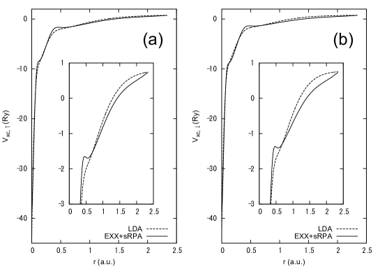
Figure 3: Exchange-correlation potentials of bcc-Fe for the EXX+sRPA (solid line) and the LDA (broken line) techniques with (a) majority spin and (b) minority spin. The insets are magnifications of the external figures. (c) and (d) are related to the correlation component of the potentials calculated for the EXX+sRPA method with (c) majority spin and (d) minority spin.

The time consumption of the calculations was approximately 10 s per iteration with one CPU core, for which 14 GFLOPS is expected at peak performance. The total calculation time, beginning with the effective atomic potentials calculated with the LDA, was typically 6 h. The values of the Green’s function were generated at 598 points in the energy plane, and 145 points in the k-space were used.

4 Conclusion

We have presented a reformulation of the OEP method. Some theoretical limitations existing in conventional derivations have been overcome by carefully considering the dependency of the energy functional on eigenvalues. Two equations, (22) and (24), are particularly important. Equation (22) suggests the existence of a correction term to the SHTS equation arising from a dependency of the energy functional on eigenvalues, which was neglected previously. Although the use of conventional equations could be justified for some exchange-correlation functionals, as we demonstrated for the LDA, EXX, and EXX+sRPA techniques in the present paper, we also showed that the RPA correlation functional offers a counterexample. Equation (24) provides a method of eliminating an unphysical degree of freedom that could be permitted in equation (22), which can be regarded as a generalized form of our previous equation[18], or the prescription proposed by KLI[9].

An efficient method of constructing a correlation potential within the EXX+sRPA approach has also been proposed. The advantage of this technique was confirmed by calculations using the model Green’s functions. We also performed realistic calculations of some transition metals, which are considered to constitute rigid test cases. In order to accelerate the calculations, we exploited the modified[18] KLI approximation[8, 9]. Although application of the modified KLI approximation would introduce some errors to the calculation, the deviations of the results from the experimental data were acceptable. Therefore, the modified KLI approximation combined with EXX+sRPA functionals is regarded as an adequate approximation for these systems at least, provided a precise technique to manage the sRPA functional is exploited.

References

- [1] R. T. Sharp and G. K. Horton. A variational approach to the unipotential many-electron problem. Phys. Rev., 90(2):317, Apr 1953.
- [2] James D. Talman and William F. Shadwick. Optimized effective atomic central potential. Phys. Rev. A, 14(1):36–40, Jul 1976.
- [3] T. Kotani. An optimized-effective-potential method for solids with exact exchange and random-phase approximation. J. Phys.: Condens. Matter, 10:9241–9261, 1998.
- [4] Stephan Kümmel and John P. Perdew. Simple iterative construction of the optimized effective potential for orbital functionals, including exact exchange. Phys. Rev. Lett., 90(4):043004, Jan 2003.
- [5] Stephan Kümmel and John P. Perdew. Optimized effective potential made simple: Orbital functionals, orbital shifts, and the exact kohn-sham exchange potential. Phys. Rev. B, 68(3):035103, Jul 2003.
- [6] K. Kosaka. Simple Iterative Procedure for Optimized Effective Potential Method in Density Functional Theory and in Current Density Functional Theory. Journal of Physical Society of Japan, 75(1):14302, 2006.
- [7] T. W. Hollins, S. J. Clark, K. Refson, and N. I. Gidopoulos. Optimized effective potential using the hylleraas variational method. Phys. Rev. B, 85:235126, Jun 2012.
- [8] J. B. Krieger, Yan Li, and G. J. Iafrate. Derivation and application of an accurate Kohn-Sham potential with integer discontinuity. Physics Letters A, 146(5):256 – 260, 1990.
- [9] J. B. Krieger, Y. Li, and G. J. Iafrate. Construction and application of an accurate local spin-polarized Kohn-Sham potential with integer discontinuity: Exchange-only theory. Phys. Rev. A, 45(1):101–126, Jan 1992.
- [10] V. N. Staroverov, G. E. Scuseria, and E. R. Davidson. Optimized effective potentials yielding Hartree–Fock energies and densities. The Journal of chemical physics, 124:141103, 2006.
- [11] V. N. Staroverov, G. E. Scuseria, and E. R. Davidson. Effective local potentials for orbital-dependent density functionals. The Journal of chemical physics, 125:081104, 2006.
- [12] A. F. Izmaylov, V. N. Staroverov, G. E. Scuseria, E. R. Davidson, G. Stoltz, and E. Cancès. The effective local potential method: Implementation for molecules and relation to approximate optimized effective potential techniques. The Journal of chemical physics, 126:084107, 2007.
- [13] A. F. Izmaylov, V. N. Staroverov, G. E. Scuseria, and E. R. Davidson. Self-consistent effective local potentials. The Journal of chemical physics, 127:084113, 2007.
- [14] O. V. Gritsenko and E. J. Baerends. Orbital structure of the kohn-sham exchange potential and exchange kernel and the field-counteracting potential for molecules in an electric field. Phys. Rev. A, 64:042506, Sep 2001.
- [15] F. Della Sala and A. Görling. Efficient localized hartree–fock methods as effective exact-exchange kohn–sham methods for molecules. The Journal of Chemical Physics, 115:5718, 2001.
- [16] J. B. Krieger, Y. Li, and G. J. Iafrate. Systematic approximations to the optimized effective potential: Application to orbital-density-functional theory. Physical Review A, 46(9):5453–5458, 1992.
- [17] T. Grabo and EKU Gross. Density-functional theory using an optimized exchange-correlation potential. Chemical Physics Letters, 240(1-3):141–150, 1995.
- [18] T. Fukazawa and H. Akai. A new practical scheme for the optimized effective potential method. Journal of Physics: Condensed Matter, 22:405501, 2010.
- [19] H. Danan, A. Herr, and A. J. P. Meyer. New determinations of the saturation magnetization of nickel and iron. Journal of Applied Physics, 39:669, 1968.
- [20] M. J. Besnus, A. J. P. Meyer, and R. Berninger. Magnetic moment measurements on fcc Co—Cu alloys. Physics Letters A, 32(3):192–193, 1970.
- [21] R. A. Reck and D. L. Fry. Orbital and spin magnetization in fe-co, fe-ni, and ni-co. Physical Review, 184(2):492–495, 1969.