Preemptive Termination of Suggestions during Sequential Kriging Optimization of a Brain Activity Reconstruction Simulation

Abstract

Reconstructing brain activity through electroencephalography requires a boundary value problem (BVP) solver to take a proposed distribution of current dipoles within the brain and compute the resulting electrostatic potential on the scalp. This article proposes the use of sequential kriging optimization to identify different optimal BVP solver parameters for dipoles located in isolated sections of the brain by considering the cumulative impact of randomly oriented dipoles within a chosen isolated section. We attempt preemptive termination of parametrizations suggested during the sequential kriging optimization which, given the results to that point, seem unlikely to produce high quality solutions. Numerical experiments on a simplification of the full geometry for which an approximate solution is available show a benefit from this preemptive termination.

1 Introduction

Electroencephalography (EEG) is a non-invasive tool for localizing neural sources and reconstructing brain activity using measurements on the surface of a patient’s scalp [22]; its practical applications involve both clinical diagnoses and neurophysical research. Maxwell’s equations explain the mechanism through which knowledge of the location and orientation of current dipoles (which model beams of active neurons) within the brain can be used to predict the resulting electrostatic potential on the scalp [23]. In practice, then, these electrostatic potentials can be measured on the scalp of a patient under some defined stimulus and an inverse problem can be solved to reconstruct the current distribution within the brain [13].

As is the case with most inverse problems, the efficiency of the solution mechanism is strongly dependent on the quality of the forward solver; for this problem, the forward solver is the boundary value problem (BVP) solver which solves Maxwell’s equation for a proposed dipole or set of dipoles which produce the boundary conditions. Possible solvers for this forward problem include the finite element method [29], the more popular boundary element method (BEM) [19] and, our preferred strategy, the method of fundamental solutions (MFS) [2].

The MFS may be preferred to FEM/BEM for its meshfree nature but it also comes with complications, primarily in the form of free parameters which may provide good or bad numerical accuracy depending on how they are chosen. Some literature describes special circumstances for which optimal MFS parameter choices are known [18], but for most problems there are only heuristic parametrization strategies for individual applications [9].

Section 1.1 details the MFS computational situation and the role that the various parameters play. In Section 2 we define a metric which measures the quality of given parameter values; we also propose a small modification to the standard sequential kriging optimization (SKO) workflow to minimize computation on underperforming parameter suggestions. Section 3 contains numerical experiments on a simplified version of the problem which show the viability of Bayesian optimization for parameter tuning in this setting.

1.1 The MFS for the Coupled BVP

The full formulation of this EEG problem using the MFS is rather involved and is discussed in full detail in [2], with [1] also providing the structure for the nearby magnetoencephalography problem. We limit this discussion to identifying the role of the free parameters in defining the MFS solution.

The MFS is popular for certain boundary value problems because it converts a boundary value problem over a volume into an approximation problem on the boundary [8]. In this situation, there are three boundary value problems, one each within the brain/skull/scalp, which must be solved in a coupled fashion to define the electrostatic potential on a patient’s scalp given a current dipole or set of dipoles within the brain. A separate solution must be defined on each of these domains,

$$u^{(r)}({\mathbf{p}})=\sum_{{\boldsymbol{\xi}}_{j}\in\Xi^{(r,\text{i})}}c_{j}^{(r,\text{i})}K({\mathbf{p}},{\boldsymbol{\xi}}_{j})+\sum_{{\boldsymbol{\xi}}_{j}\in\Xi^{(r,\text{d})}}c_{j}^{(r,\text{d})}K({\mathbf{p}},{\boldsymbol{\xi}}_{j}),$$

for $r=1,2,3$ corresponding to the scalp, skull and brain, respectively. and each of these solutions has free parameters, Here, $K({\mathbf{p}},{\boldsymbol{\xi}})=1/\|{\mathbf{p}}-{\boldsymbol{\xi}}\|$ is the Green’s kernel for the three dimensional Laplacian on an unbounded domain [12]. Our free parameters appear in the construction of the so-called fictitious boundary on which the sets of kernel centers $\Xi$ are defined; we use $\Xi^{(1,\text{i})}$ to denote the kernel centers on the inflated fictitious boundary associated with the scalp solution and $\Xi^{(1,\text{d})}$ to define the kernel centers on the scalp’s deflated fictitious boundary. The allocation and placement of source points has been a complication for MFS methods since their inception and was discussed at length in a recent survey [9]. Figure 1 depicts the computational setup for this problem.

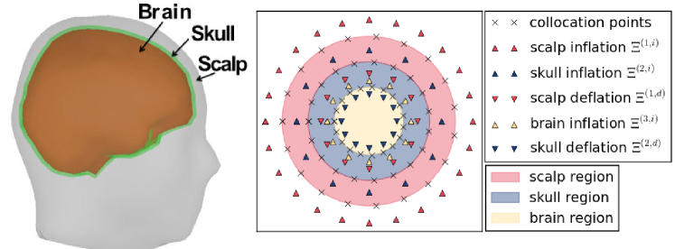
Figure 1: left: Depiction of the components of the reconstruction problem. right: Distribution of MFS points on a more easily readable simplification of the domain.

Following the problem definition in [2], each fictitious boundary is defined with an inflation or deflation parameter, and the size of the set of kernel centers $\Xi$ associated with that fictitious boundary, $|\Xi|$, must also be chosen. Thus, in this formulation, there are as many as 10 free parameters defining the solution to this coupled BVP, two for each fictitious boundary/interface. However, because there is often a desire to balance the number of kernel centers and collocation points, we fix values for the number of centers $|\Xi|$ and instead attempt to only adjust the inflation/deflation of the 5 fictitious boundaries. We hope to use future work to simultaneously select both aspects of the BVP solver.

2 Sequential Kriging Optimization for Tuning MFS EEG Solvers

Sequential kriging optimization [14] as well as related terms and methods such as hyperparameter selection [5], sequential model-based algorithm configuration [15] or the ultimately general Bayesian optimization [27], provide strategies for efficiently optimizing black-box functions. To more clearly state our black-box function, we assume only a single dipole ${\mathbf{p}}^{\prime}$ exists within the brain; this distinction would need to be lifted to apply this method in the full spectrum of possible EEG reconstructions.

The black box function we define here is based on the goal of identifying optimal free parameters for an MFS solution as the forward solver within an inverse solver so as to make the inverse solver as efficient and accurate as possible. We define the quality of a set of parameters ${\boldsymbol{\theta}}$ for a single dipole ${\mathbf{p}}^{\prime}$ as the difference between the MFS and true solutions for that ${\mathbf{p}}^{\prime}$ at a set of test points on the scalp. We compress this difference into a scalar with

$$Q({\boldsymbol{\theta}};{\mathbf{p}}^{\prime})=-\log\left(\sum_{k=1}^{{k_{\text{test}}}}\left|u_{\text{MFS}}^{(1)}({\mathbf{p}}_{k})-u_{\text{true}}^{(1)}({\mathbf{p}}_{k})\right|^{2}\;\Big{/}\;\sum_{k=1}^{{k_{\text{test}}}}\left|u_{\text{true}}^{(1)}({\mathbf{p}}_{k})\right|^{2}\right),$$ (1)

where ${k_{\text{test}}}$ represents the number of ${\mathbf{p}}_{k}$ test points placed on the scalp. The dipole ${\mathbf{p}}^{\prime}$ appears implicitly in the definition of the $c$ terms in the $u_{\text{MFS}}$ solution as well as in the “true” solution.

Dipoles in different brain regions will likely require different inflation/deflation of the fictitious boundary to perform optimally. We propose that, within a given region $\Omega^{\prime}$ of the brain, dipoles be selected with random location and orientation and then we study the mean performance over those dipoles. If we abuse notation slightly and define the uniform sampling of dipole locations and orientations within $\Omega^{\prime}$ as ${\mathbf{p}}^{\prime}\sim\operatorname*{Unif}(\Omega^{\prime})$, we can denote the sample mean over ${n_{\text{avg}}}$ observations as $\bar{Q}({\boldsymbol{\theta}})$; this sample average is the black-box function to be maximized during the SKO. We also use the sample variance in the construction of the kriging model [25].

Algorithm 1 Preemptive EEG Termination

  Input: $\Omega^{\prime},{j_{\text{max}}},{n_{\text{avg}}},{n_{\text{min}}},{j_{\text{init}}}$

  $j\leftarrow 0;\mathcal{R}\leftarrow\{\};$

  while $j<{j_{\text{max}}}$ do

     ${\boldsymbol{\theta}}\leftarrow\text{suggestion\_{}from\_{}SKO}(\mathcal{R})$

     ${\mathbf{v}}\leftarrow\{\}$

     for $n\leftarrow 0$ to ${n_{\text{avg}}}$ do

        ${\mathbf{p}}^{\prime}\sim\operatorname*{Unif}(\Omega^{\prime})$

        ${\mathbf{v}}\leftarrow{\mathbf{v}}\cup Q({\boldsymbol{\theta}};{\mathbf{p}}^{\prime})$

        $j\leftarrow j+1$

        if $n>{n_{\text{min}}}$ and $j>{j_{\text{init}}}$ then

           break if $\operatorname*{Mean}({\mathbf{v}})<\operatorname*{Mean}(\mathcal{R})$

        end if

     end for

     $\mathcal{R}\leftarrow\mathcal{R}\cup\{{\boldsymbol{\theta}},{\mathbf{v}}\}$

  end while

In initial SKO experiments, we recognized that for ${\mathbf{p}}^{\prime}\sim\operatorname*{Unif}(\Omega^{\prime})$ most ${\boldsymbol{\theta}}$ yielded similar distribution shapes of $Q({\boldsymbol{\theta}};{\mathbf{p}}^{\prime})$ values differing primarily by their mean. This led us to believe that, since the impact of ${\boldsymbol{\theta}}$ was primarily a translation of the $\bar{Q}$ distribution, we could predict with fewer than ${n_{\text{avg}}}$ values of ${\mathbf{p}}^{\prime}\sim\operatorname*{Unif}(\Omega^{\prime})$ whether a given ${\boldsymbol{\theta}}$ could perform optimally.

We implemented a heuristic strategy which is on display in Algorithm 1. This algorithm requires choosing preemption parameters: ${j_{\text{max}}}$ is the total number of MFS/true solutions to be computed over the course of the optimization, ${n_{\text{avg}}}$ is the maximum number of ${\mathbf{p}}^{\prime}$ choices to consider before returning $\bar{Q}({\boldsymbol{\theta}})$, ${n_{\text{min}}}$ is the minimum number of ${\mathbf{p}}^{\prime}$ choices to consider before allowing preemptive termination, and ${j_{\text{init}}}$ is the number of initial $Q$ evaluations for which preemption is forbidden so as to form a baseline of $Q$ values. We write $\operatorname*{Mean}(\mathcal{R})$ to denote the mean of the scores of all the ${\mathbf{p}}^{\prime}$ considered thus far when pooled into a single sample, i.e., if $\mathcal{R}=\{\{{\boldsymbol{\theta}}_{1},\{1,2,3\}\},\{{\boldsymbol{\theta}}_{2},\{4,5,6\}\}\}$ then $\operatorname*{Mean}(\mathcal{R})=3.5$. Any partially completed ${\boldsymbol{\theta}}$ values still report their $\bar{Q}$ and sample variance values to the kriging model.

This concept of a variable amount of work depending on the perceived quality of a given suggestion appears under various names in the literature such as freeze-thaw Bayesian optimization [28], hyperband [20], or predictive termination [10]. Similarly to our strategy, the F-Race Algorithm [7] (which has an open source implementation [21]) provides a mechanism for allowing multiple parallel suggestions and a statistical analysis for discarding underperforming suggested ${\boldsymbol{\theta}}$. Similar racing and adaptive capping methods are also available in the open source software ParamILS [16]. The literature on multi-armed or infinitely-armed bandits may also provide a more rigorous mechanism for pausing and revisiting a range of ${\boldsymbol{\theta}}$ suggestions in a regret-based framework, rather than terminating suggestions as described in Algorithm 1 [3]. Of immediate interest to our SKO framework is the use of covariance kernels which contain components modeling the quality of the approximation $\bar{Q}$ as a function of $n$ (and, perhaps, a bootstrap estimate of the variance [11]) which is a topic that has appeared in some uncertainty quantification research [24]. While our heuristic is simple to state and implement, it will be improved upon and augmented in future work using this rich breadth of available ideas present in the optimization and model configuration communities.

3 Numerical Experiments

To simplify initial testing and isolate potential sources of error/uncertainty, these numerical experiments involve a less complicated geometry for which there exists an analytic solution [30]: three concentric spheres (of radii .087, .092 and .1 m with conductivity .33, .0125 and .33 S/m respectively) replace the physical brain/skull/scalp geometry we eventually hope to use. Refer to Figure 1 to see how the source points are distributed in this domain. Future work must involve the more realistic geometries explored in [2].

All dipole moments have magnitude 1 A$\cdot$m. The SKO used an expected improvement acquisition function [17]; any ${\boldsymbol{\theta}}$ values that yielded a collocation matrix without full rank were treated as failures. These experiments used values of ${k_{\text{test}}}=1000$, ${j_{\text{max}}}=800$, ${n_{\text{avg}}}=30$, ${n_{\text{min}}}=5$ and ${j_{\text{init}}}=5{n_{\text{avg}}}$; for these parameters, the maximum number of non-failed ${\boldsymbol{\theta}}$ values which can be considered (which only occurs in the case where they produce increasingly low $\bar{Q}$) is ${j_{\text{init}}}/{n_{\text{max}}}+({j_{\text{max}}}-{j_{\text{init}}})/{n_{\text{min}}}=135$ and the minimum number to be considered (which only occurs for increasingly high $\bar{Q}$) is ${j_{\text{init}}}/{n_{\text{max}}}+({j_{\text{max}}}-{j_{\text{init}}})/{n_{\text{max}}}\approx 27$. The parameter values suggested here are chosen arbitrarily, although ${n_{\text{min}}}=5$ was provide some opportunity to perform before truncation. All point distributions on spheres are created with the spiral method described in [26]. The number of collocation points on each of the three spheres was always fixed at 300, with $|\Xi^{(1,d)}|=|\Xi^{(2,i)}|=|\Xi^{(2,d)}|=|\Xi^{(3,i)}|=90$ and $|\Xi^{(1,i)}|=180$; these choices were made arbitrarily, and future work could include tuning these values along with the inflation/deflation parameters. Test results are presented in Table 1.

Table 1: Median results over 30 tests from specific dipole distributions. Preemptive and standard refer to whether or not ${n_{\text{min}}}<{n_{\text{avg}}}$ or ${n_{\text{min}}}={n_{\text{avg}}}$, respectively. Bonus states the number of extra suggestions enjoyed by the preemptive strategy; for example, a Bonus 10 value states that 10 additional ${\boldsymbol{\theta}}$ parameters were able to be tested because the preemptive truncation allowed for as few as ${n_{\text{min}}}$ MFS solves to be conducted rather than the full ${n_{\text{avg}}}$. Preemptive results in italics indicate a statistically significant difference with $p<.05$ from Standard using a Mann-Whitney $U$ test.

Index	Sequential Kriging Optimiztion			Random Search
	Standard	Preemptive	Bonus	Standard	Preemptive	Bonus
1	3.681	3.845	16	3.631	3.439	27
2	1.494	1.532	15	1.333	1.383	30
3	5.090	5.245	10	4.672	4.905	19
4	0.862	0.978	28	0.778	0.870	34
5	0.219	0.257	21	0.146	0.195	30
6	2.131	2.209	21	1.944	2.058	31

At https://github.com/sigopt/sigopt-examples there is a description of the dipole regions associated with each index. As evidenced by the range of optimal $\bar{Q}$ values found, the tests vary in difficulty; however, in each test there is a benefit to using SKO over basic random search [6], and a benefit to using the preemption strategy outlined in Section 2.

Acknowledgments

We would like to present our thanks to the organizers of this workshop, and especially to Roberto Calandra who has been very helpful and supportive throughout this process. We also would like to thank the anonymous referee whose in depth comments and comprehensive references have greatly improved our presentation and have provided us with numerous future paths for which to improve this research.

References

- [1] G. Ala, G. E. Fasshauer, E. Francomano, S. Ganci, and M. J. McCourt. A meshfree solver for the MEG forward problem. IEEE Transactions on Magnetics, 51(3):5000304, 2015.
- [2] G. Ala, G. E. Fasshauer, E. Francomano, S. Ganci, and M. J. McCourt. The method of fundamental solutions in solving coupled boundary value problems for M/EEG. SIAM Journal on Scientific Computing, 37(4):B570–B590, 2015.
- [3] Peter Auer. Using confidence bounds for exploitation-exploration trade-offs. Journal of Machine Learning Research, 3(Nov):397–422, 2002.
- [4] AH Barnett and Timo Betcke. Stability and convergence of the method of fundamental solutions for Helmholtz problems on analytic domains. Journal of Computational Physics, 227(14):7003–7026, 2008.
- [5] J. S. Bergstra, R. Bardenet, Y. Bengio, and B. Kégl. Algorithms for hyper-parameter optimization. In Advances in Neural Information Processing Systems, pages 2546–2554, 2011.
- [6] James Bergstra and Yoshua Bengio. Random search for hyper-parameter optimization. Journal of Machine Learning Research, 13(Feb):281–305, 2012.
- [7] Mauro Birattari, Zhi Yuan, Prasanna Balaprakash, and Thomas Stützle. F-Race and iterated F-Race: An overview. In Experimental methods for the analysis of optimization algorithms, pages 311–336. Springer, 2010.
- [8] Ching-Shyang Chen, Andreas Karageorghis, and Yiorgos S Smyrlis. The method of fundamental solutions: a meshless method. Dynamic Publishers Atlanta, GA, 2008.
- [9] CS Chen, A Karageorghis, and Yan Li. On choosing the location of the sources in the MFS. Numerical Algorithms, 72(1):107–130, 2016.
- [10] Tobias Domhan, Jost Tobias Springenberg, and Frank Hutter. Speeding up automatic hyperparameter optimization of deep neural networks by extrapolation of learning curves. In Proceedings of the 24th International Joint Conference on Artificial Intelligence (IJCAI), 2015.
- [11] Bradley Efron. Nonparametric estimates of standard error: the jackknife, the bootstrap and other methods. Biometrika, 68(3):589–599, 1981.
- [12] Graeme Fairweather and Andreas Karageorghis. The method of fundamental solutions for elliptic boundary value problems. Advances in Computational Mathematics, 9(1-2):69–95, 1998.
- [13] R. Grech, T. Cassar, J. Muscat, K. Camilleri, S. Fabri, M. Zervakis, P. Xanthopoulos, V. Sakkalis, and B. Vanrumste. Review on solving the inverse problem in EEG source analysis. Journal of NeuroEngineering and Rehabilitation, 5(25), 2008.
- [14] D. Huang, T. T. Allen, W. I. Notz, and N. Zeng. Global optimization of stochastic black-box systems via sequential kriging meta-models. Journal of Global Optimization, 34(3):441–466, 2006.
- [15] Frank Hutter, Holger H Hoos, and Kevin Leyton-Brown. Sequential model-based optimization for general algorithm configuration. In Learning and Intelligent Optimization, pages 507–523. Springer, 2011.
- [16] Frank Hutter, Holger H. Hoos, Kevin Leyton-Brown, and Thomas Stützle. ParamILS: an automatic algorithm configuration framework. Journal of Artificial Intelligence Research, 36:267–306, October 2009.
- [17] D. R. Jones, M. Schonlau, and W. J. Welch. Efficient global optimization of expensive black-box functions. Journal of Global optimization, 13(4):455–492, 1998.
- [18] Masashi Katsurada. Asymptotic error analysis of the charge simulation method in a jordan region with an analytic boundary. J. Fac. Sci. Univ. Tokyo Sect. IA Math, 37(3):635–657, 1990.
- [19] Jan Kybic, Maureen Clerc, Touffic Abboud, Olivier Faugeras, Renaud Keriven, and Théodore Papadopoulo. A common formalism for the integral formulations of the forward EEG problem. IEEE transactions on medical imaging, 24(1):12–28, 2005.
- [20] Lisha Li, Kevin Jamieson, Giulia DeSalvo, Afshin Rostamizadeh, and Ameet Talwalkar. Efficient hyperparameter optimization and infinitely many armed bandits. In ICML 2016 workshop on AutoML (AutoML 2016), 2016.
- [21] Manuel López-Ibáñez, Jérémie Dubois-Lacoste, Leslie Pérez Cáceres, Mauro Birattari, and Thomas Stützle. The irace package: Iterated racing for automatic algorithm configuration. Operations Research Perspectives, 3:43–58, 2016.
- [22] E. Niedermeyer and F.L. da Silva. Electroencephalography: Basic Principles, Clinical Applications, and Related Fields. Lippincott Williams & Wilkins, 2012.
- [23] P.L. Nunez and R. Srinivasan. Electric Fields of the Brain: The Neurophysics of EEG. Oxford University Press, 2006.
- [24] Victor Picheny and David Ginsbourger. A nonstationary space-time Gaussian process model for partially converged simulations. SIAM/ASA Journal on Uncertainty Quantification, 1(1):57–78, 2013.
- [25] C. E. Rasmussen and C. Williams. Gaussian Processes for Machine Learning. MIT Press, Cambridge, MA, 2006.
- [26] Edward B Saff and A BJ Kuijlaars. Distributing many points on a sphere. The mathematical intelligencer, 19(1):5–11, 1997.
- [27] Jasper Snoek, Hugo Larochelle, and Ryan P Adams. Practical bayesian optimization of machine learning algorithms. In Advances in neural information processing systems, pages 2951–2959, 2012.
- [28] Kevin Swersky, Jasper Snoek, and Ryan Prescott Adams. Freeze-thaw bayesian optimization. arXiv preprint arXiv:1406.3896, 2014.
- [29] C.H. Wolters, H. Köstler, C. Möller, J. Härdtlein, L. Grasedyck, and W. Hackbusch. Numerical mathematics of the subtraction method for the modeling of a current dipole in EEG source reconstruction using finite element head models. SIAM Journal on Scientific Computing, 30(1):24–45, 2008.
- [30] Zhi Zhang. A fast method to compute surface potentials generated by dipoles within multilayer anisotropic spheres. Physics in medicine and biology, 40(3):335, 1995.