Experimental detection of nonclassicality of single-mode fields via intensity moments

Abstract

Nonclassicality criteria based on intensity moments and derived from the usual matrix approach are compared to those provided by the majorization theory. The majorization theory is shown to give a greater number of more suitable nonclassicality criteria. Fifteen experimentally useful criteria of the majorization theory containing the intensity moments up to the fifth order are identified. Their performance is experimentally demonstrated on the set of eleven potentially nonclassical states generated from a twin beam by postselection based on detecting a given number of photocounts in one arm by using an iCCD camera.

1 Introduction

The world of quantum states of optical fields was discovered soon after the construction of the first laser that opened the area of nonlinear optics [1] for extensive investigations. The experimental effort has been supported by the fast development of theory [2] that provided soon the crucial coherent states, the Glauber-Sudarshan representation of the statistical operator and quantum generalization of the coherence theory [3, 4]. The Glauber-Sudarshan representation also brought a clear and strict definition of nonclassical optical states [3]: A quantum state of an optical field is nonclassical if and only if the Glauber-Sudarshan representation of its statistical operator fails to be a probability density (it attains negative values or even does not exist as a regular function). Applying this definition, a huge amount of quantum states can be identified. From the point of view of the fundamental physical importance, three distinct kinds of such states have attracted the greatest attention of experimentalists from the very beginning [5]: squeezed states with reduced phase fluctuations, sub-Poissonian states with reduced intensity (or photon-number) fluctuations and anti-bunched light with unusual temporal correlations.

The verification of nonclassicality of an optical state can be done directly from its definition given in the above paragraph, provided that its statistical operator is reconstructed from the measured data. However, this requires in general the application of homodyne tomography [6] or homodyne detection [7], which is experimentally demanding. Qualitative simplification is reached only for optical fields with the uniform distribution of phases for which the measurement of photocount statistics is sufficient to reconstruct the quasi-distribution of integrated intensities [8, 9, 10, 11, 12] that fully characterizes the field. We note that even the full state reconstruction can be reached using only the photocount statistics in some specific cases, e.g., for a two-mode Gaussian field without coherent contributions [13]. Because of the complexity of state reconstruction, alternative approaches for revealing the nonclassicality of a state have been looked for, even considering transformations of the nonclassicality into its different forms [14, 15, 16]. A large number of various inequalities comprising both moments of amplitudes and intensities of different orders have been derived [17, 18, 19, 20, 21] and experimentally tested [22, 23, 24, 25]. A unifying matrix approach for their derivation has been formulated relying on nonnegativity of classical quadratic forms defined above amplitude and intensity powers of different orders [26, 27, 28]. Different inequalities have been compared in [29]. Even more general forms of such inequalities have been reached applying the Bochner theorem [30, 31]. There also exists a completely different approach for the derivation of such inequalities based on the mathematical theory of majorization [32, 33].

Inequalities containing only moments of intensities are frequently used to reveal the nonclassicality of experimentally investigated states, contrary to those written for amplitude moments. This is natural, as the measurement of amplitude moments requires the homodyne scheme [5] whose complexity of implementation is comparable to the homodyne tomography. On the other hand, intensity moments can be obtained with the usual ’quadratic’ optical detectors or, for low intensities, with their modern variants resolving individual photon numbers [34]. In this contribution, we compare the nonclassicality inequalities derived from the matrix approach with those provided by the majorization theory using a set of sub-Poissonian states with increasing mean photon numbers [35]. These states are generated from a twin beam [36] by postselection [37, 38] that is based on the detection of a given photocount number in one arm of the twin beam by an intensified charge-coupled-device (iCCD) camera [39]. The iCCD camera is also used to experimentally analyze the sub-Poissonian states with mean photon numbers ranging from 7 to 14.

The paper is organized as follows. In Sec. 2, systematic approach for the derivation of nonclassicality inequalties is given using both the matrix approach and the majorization theory. Inequalities derived in Sec. 2 are tested on the experimental data in Sec. 3. Sec. 4 brings conclusions.

2 Derivation of nonclassicality inequalities

For the moments of classical integrated intensity $I$ [8], a general nonnegative quadratic form for the classical field is constructed via the function $g(I)$ that is an arbitrary linear superposition of the terms $I^{j}$ for $j=0,1,\ldots$:

$$g(I)=\sum_{j=0}^{N}g_{j}I^{j},$$ (1)

and $N$ is an arbitrary integer number giving the number of terms in the sum. The condition $\int_{0}^{\infty}dI\,P(I)|g(I)|^{2}\geq 0$ for a classical state with non-negative probability function $P$, when transformed into the operator form written for the powers of photon-number operator $\hat{n}$ ($I^{j}\propto$ $:\hat{n}^{j}\!:$), suggests the following nonclassicality condition [26, 27, 28, 29]:

$$\sum_{j,j^{\prime}=0}^{N}g_{j}g_{j^{\prime}}\langle:\!\hat{n}^{j+j^{\prime}}\!:\rangle<0;$$ (2)

symbol $:\>:$ denotes normal ordering of field operators. Inequality (2) can be equivalently expressed as the condition for negativity of a matrix ${M}$ of dimension $(N+1)\times(N+1)$ with the elements $M_{jj^{\prime}}=\langle:\!\hat{n}^{j+j^{\prime}}\!:\rangle$. The Hurwitz criterion then guarantees negativity of the matrix ${M}$ whenever any of its principal minors is negative.

The simplest $2\times 2$ minors of the matrix ${M}$ written as

$${\rm det}\left[\begin{array}[]{cc}\langle:\!\hat{n}^{2k}\!:\rangle&\langle:\!\hat{n}^{k+l}\!:\rangle\cr\langle:\!\hat{n}^{k+l}\!:\rangle&\langle:\!\hat{n}^{2l}\!:\rangle\end{array}\right]$$ (3)

provide the nonclassicality inequalities containing the products of two moments of in general different orders:

$$\langle:\!\hat{n}^{2k}\!:\rangle\langle:\!\hat{n}^{2l}\!:\rangle<\langle:\!\hat{n}^{k+l}\!:\rangle^{2},\hskip 14.22636pt0\leq k\leq l.$$ (4)

The $3\times 3$ minors of matrix ${M}$ parameterized by integer numbers $k$, $l$ and $m$ already give more complex nonclassicality inequalities involving in general 6 terms in the sum, each formed by three moments in the product:

$${\rm det}\left[\begin{array}[]{ccc}\langle:\!\hat{n}^{2k}\!:\rangle&\langle:\!\hat{n}^{k+l}\!:\rangle&\langle:\!\hat{n}^{k+m}\!:\rangle\cr\langle:\!\hat{n}^{k+l}\!:\rangle&\langle:\!\hat{n}^{2l}\!:\rangle&\langle:\!\hat{n}^{l+m}\!:\rangle\cr\langle:\!\hat{n}^{k+m}\!:\rangle&\langle:\!\hat{n}^{l+m}\!:\rangle&\langle:\!\hat{n}^{2m}\!:\rangle\cr\end{array}\right]<0,\hskip 14.22636pt0\leq k\leq l\leq m.$$ (8)

The form of nonclassicality inequalities originating in $k\times k$ minors for $k>3$ is similar to that derived for the $3\times 3$ minors.

On the other hand, the majorization theory [32] gives us the nonclassicality inequalities involving two moments in the product and having the following form [33]:

$$\tilde{R}_{u,v}^{u+m,v-m}\equiv\langle:\!\hat{n}^{u+m}\!:\rangle\langle:\!\hat{n}^{v-m}\!:\rangle-\langle:\!\hat{n}^{u}\!:\rangle\langle:\!\hat{n}^{v}\!:\rangle<0,\hskip 14.22636ptu\geq v\geq 0,\;v\geq m\geq 0.$$ (9)

The inequalities written in Eq. (4) are a subset of those given in Eq. (9) with the mapping $u=v=k+l$ and $m=l-k$.

The following nonclassicality inequalities of the majorization theory represent the counterpart of inequalities in Eq. (9) derived from the $3\times 3$ minors:

$$\tilde{R}_{u,v,w}^{u+k+l,v-k+m,w-l-m} \equiv \langle:\!\hat{n}^{u+k+l}\!:\rangle\langle:\!\hat{n}^{v-k+m}\!:\rangle\langle:\!\hat{n}^{w-l-m}\!:\rangle-\langle:\!\hat{n}^{u}\!:\rangle\langle:\!\hat{n}^{v}\!:\rangle\langle:\!\hat{n}^{w}\!:\rangle<0,$$ (10)

$$\hskip 14.22636ptu\geq v\geq w\geq 0;\hskip 14.22636pt\;k,l,m\geq 0.$$

Inequalities in Eq. (10) formed by two additive terms differ from those of Eq. (8) that contain six additive terms. There does not seem to exist any simple relation between inequalities written in Eqs. (10) and (8).

In general, the majorization theory provides a larger number of nonclassicality inequalities compared to the matrix approach. Moreover these inequalities attain a simpler form [compare Eqs. (8) and (10)]. To get a more detailed comparison of the two methods, we write down explicitly the inequalities involving the moments with the overall power up to five, that are useful for the experimental analysis below. The explicit formulas of Eq. (9) written in their normalized (dimensionless) form are expressed as follows:

$$R_{1,1}^{2,0} \equiv \frac{\langle:\!\hat{n}^{2}\!:\rangle}{\langle:\!\hat{n}\!:\rangle^{2}}-1<0,$$

$$R_{2,1}^{3,0} \equiv \frac{\langle:\!\hat{n}^{3}\!:\rangle}{\langle:\!\hat{n}\!:\rangle^{3}}-\frac{\langle:\!\hat{n}^{2}\!:\rangle}{\langle:\!\hat{n}\!:\rangle^{2}}<0,$$

$$R_{2,2}^{3,1} \equiv \frac{\langle:\!\hat{n}^{3}\!:\rangle}{\langle:\!\hat{n}\!:\rangle^{3}}-\frac{\langle:\!\hat{n}^{2}\!:\rangle^{2}}{\langle:\!\hat{n}\!:\rangle^{4}}<0,$$

$$R_{2,2}^{4,0} \equiv \frac{\langle:\!\hat{n}^{4}\!:\rangle}{\langle:\!\hat{n}\!:\rangle^{4}}-\frac{\langle:\!\hat{n}^{2}\!:\rangle^{2}}{\langle:\!\hat{n}\!:\rangle^{4}}<0,$$

$$R_{3,1}^{4,0} \equiv \frac{\langle:\!\hat{n}^{4}\!:\rangle}{\langle:\!\hat{n}\!:\rangle^{4}}-\frac{\langle:\!\hat{n}^{3}\!:\rangle}{\langle:\!\hat{n}\!:\rangle^{3}}<0,$$

$$R_{4,1}^{5,0} \equiv \frac{\langle:\!\hat{n}^{5}\!:\rangle}{\langle:\!\hat{n}\!:\rangle^{5}}-\frac{\langle:\!\hat{n}^{4}\!:\rangle}{\langle:\!\hat{n}\!:\rangle^{4}}<0,$$

$$R_{3,2}^{4,1} \equiv \frac{\langle:\!\hat{n}^{4}\!:\rangle}{\langle:\!\hat{n}\!:\rangle^{4}}-\frac{\langle:\!\hat{n}^{2}\!:\rangle\langle:\!\hat{n}^{3}\!:\rangle}{\langle:\!\hat{n}\!:\rangle^{5}}<0,$$

$$R_{3,2}^{5,0} \equiv \frac{\langle:\!\hat{n}^{5}\!:\rangle}{\langle:\!\hat{n}\!:\rangle^{5}}-\frac{\langle:\!\hat{n}^{2}\!:\rangle\langle:\!\hat{n}^{3}\!:\rangle}{\langle:\!\hat{n}\!:\rangle^{5}}<0.$$ (11)

Only the first and the fourth inequalities in Eq. (11) stem from the matrix approach providing Eq. (4). Similarly, the general formula in Eq. (10) leaves us with the following four normalized inequalities, which cannot be obtained from the matrix approach:

$$R_{1,1,1}^{3,0,0} \equiv \frac{\langle:\!\hat{n}^{3}\!:\rangle}{\langle:\!\hat{n}\!:\rangle^{3}}-1<0,$$

$$R_{2,1,1}^{4,0,0} \equiv \frac{\langle:\!\hat{n}^{4}\!:\rangle}{\langle:\!\hat{n}\!:\rangle^{4}}-\frac{\langle:\!\hat{n}^{2}\!:\rangle}{\langle:\!\hat{n}\!:\rangle^{2}}<0,$$

$$R_{2,2,1}^{5,0,0} \equiv \frac{\langle:\!\hat{n}^{5}\!:\rangle}{\langle:\!\hat{n}\!:\rangle^{5}}-\frac{\langle:\!\hat{n}^{2}\!:\rangle^{2}}{\langle:\!\hat{n}\!:\rangle^{4}}<0,$$

$$R_{3,1,1}^{5,0,0} \equiv \frac{\langle:\!\hat{n}^{5}\!:\rangle}{\langle:\!\hat{n}\!:\rangle^{5}}-\frac{\langle:\!\hat{n}^{3}\!:\rangle}{\langle:\!\hat{n}\!:\rangle^{3}}<0.$$ (12)

The majorization theory gives us also inequalities containing four (five) moments in the product, which encompass the following two (one) inequalities useful in our experimental analysis:

$$R_{1,1,1,1}^{4,0,0,0} \equiv \frac{\langle:\!\hat{n}^{4}\!:\rangle}{\langle:\!\hat{n}\!:\rangle^{4}}-1<0,$$

$$R_{2,1,1,1}^{5,0,0,0} \equiv \frac{\langle:\!\hat{n}^{5}\!:\rangle}{\langle:\!\hat{n}\!:\rangle^{5}}-\frac{\langle:\!\hat{n}^{2}\!:\rangle}{\langle:\!\hat{n}\!:\rangle^{2}}<0,$$

$$R_{1,1,1,1,1}^{5,0,0,0,0} \equiv \frac{\langle:\!\hat{n}^{5}\!:\rangle}{\langle:\!\hat{n}\!:\rangle^{5}}-1<0.$$ (13)

The above inequalities can be applied both to photon-number distributions as well as to photocount distributions that are directly measured. Whereas the normally-ordered moments of photon number $\hat{n}$ are suitable for characterizing intensity distributions, the usual moments are immediately derived from the experimental photocount distributions. They are mutually related by the following formula [8]:

$$\langle:\!\hat{n}^{k}\!:\rangle=\left\langle\frac{\hat{n}!}{(\hat{n}-k)!}\right\rangle.$$ (14)

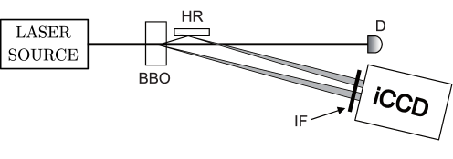
Figure 1: Scheme of the experiment generating sub-Poissonian states. A twin beam is generated in noncollinear geometry in a 5-mm-long type-I barium-borate crystal (BaB₂O₄, BBO) pumped by the third harmonics (280 nm) of a femtosecond cavity dumped Ti:sapphire laser (pulse duration 150 fs, central wavelength 840 nm). The signal field as well as the idler field (after reflection on a highly-reflecting mirror HR) are detected by $N_{\rm s}=6528$ and $N_{\rm i}=6784$ pixels of the photocathode of iCCD camera Andor DH3345-18U-63 with dark-count rate $d=0.04$ ($D_{a}=d/N_{a}$, $a={\rm s,i}$). The nearly-frequency-degenerate signal and idler photons at the wavelength of 560 nm are filtered by a 14-nm-wide bandpass interference filter IF. Intensity of the pump beam that is actively stabilized via a motorized half-wave plate followed by a polarizer is monitored by detector D.

3 Experimental testing of nonclassicality inequalities

The above nonclassicality inequalities have been applied to a set of states with different ’degree’ of sub-Poissonian photon-number statistics that were generated from a twin beam using postselection based on the detection of a given number $c_{\rm s}$ of photocounts in the signal field [35]. For an ideal photon-number-resolving detector, detection of a given number $c_{\rm s}$ of signal photocounts leaves the idler field in the Fock state with $c_{\rm s}$ photons. For a real photon-number-resolving detector, an idler field with reduced photon-number fluctuations and potentially sub-Poissonian photon-number statistics is obtained. As the mean number of idler photons in a postselected field increases with the increasing signal photocount number $c_{\rm s}$, the set of generated states is appealing for testing the power of the nonclassicality inequalities.

In the reported experiment, the twin beam was generated in a nonlinear crystal and both its signal and idler fields were detected by an iCCD camera [11]. Whereas the signal photocounts were used for the postselection process, the histograms of idler photocounts provided the information about the postselected potentially sub-Poissonian idler fields. Experimental details are written in the caption to Fig. 1. The experiment was repeated $1.2\times 10^{6}$ times. The obtained 2D histogram of the signal and idler photocounts was used both to determine the photocount moments occurring in the nonclassicality inequalities and to reconstruct the photon-number distributions of the postselected idler fields by the method of maximum likelihood [40]. In the reconstruction method, the idler-field conditional photon-number distribution $p_{\rm c,i}(n_{\rm i};c_{\rm s})$ left after detecting $c_{\rm s}$ signal photocounts is reached as a steady state found in the following iteration procedure (with iteration index $n$) [11]

$$p_{\rm c,i}^{(n+1)}(n_{\rm i};c_{\rm s})=p_{\rm c,i}^{(n)}(n_{\rm i};c_{\rm s})\sum_{c_{\rm i}}\frac{f_{\rm i}(c_{\rm i};c_{\rm s})T_{\rm i}(c_{\rm i},n_{\rm i})}{\sum_{n^{\prime}_{i}}T_{\rm i}(c_{\rm i},n^{\prime}_{\rm i})p_{\rm c,i}^{(n)}(n^{\prime}_{\rm i};c_{\rm s})}$$ (15)

that uses the normalized idler-field 1D photocount histogram $f_{\rm i}(c_{\rm i};c_{\rm s})\equiv\frac{f(c_{\rm s},c_{\rm i})}{\sum\limits_{c_{\rm i}}f(c_{\rm s},c_{\rm i})}$ built from the detections with $c_{\rm s}$ detected signal photocounts and contained in the joint signal-idler photocount histogram $f(c_{\rm s},c_{\rm i})$. In Eq. (15), the functions $T(c_{\rm i},n_{\rm i})$ give the probabilities of having $c_{\rm i}$ photocounts when detecting a field with $n_{\rm i}$ photons. The folowing formula was derived for an iCCD camera with $N_{a}$ active pixels, detection efficiency $\eta_{a}$ and dark-count rate per pixel $D_{a}$ [11]:

$$T_{a}(c_{a},n_{a}) = \left(\begin{array}[]{c}N_{a}\\ c_{a}\end{array}\right)(1-D_{a})^{N_{a}}(1-\eta_{a})^{n_{a}}(-1)^{c_{a}}\sum_{l=0}^{c_{a}}\left(\begin{array}[]{c}c_{a}\\ l\end{array}\right)\frac{(-1)^{l}}{(1-D_{a})^{l}}$$ (21)

$$\mbox{}\times\left(1+\frac{l}{N_{a}}\frac{\eta_{a}}{1-\eta_{a}}\right)^{n_{a}};\hskip 28.45274pta={\rm s,i}.$$

The 2D histogram $f(c_{\rm s},c_{\rm i})$ with $\langle c_{\rm s}\rangle=2.20$ and $\langle c_{\rm i}\rangle=2.18$ signal and idler mean photocounts, respectively, also allowed to reconstruct the whole original twin beam in the form of multimode Gaussian fields composed of the independent multimode paired, signal and idler parts characterized by mean photon(-pair) numbers $B_{a}$ per mode and numbers $M_{a}$ of independent modes, $a={\rm p,s,i}$ [12]. The photon-nunber distribution $p_{\rm si}(n_{\rm s},n_{\rm i})$ of the whole twin beam was expressed in the form of a two-fold convolution of three Mandel-Rice photon-number distributions [8] in this case [41, 12, 42]:

$$p_{\rm si}(n_{\rm s},n_{\rm i})=\sum_{n=0}^{{\rm min}[n_{\rm s},n_{\rm i}]}p(n_{\rm s}-n;M_{\rm s},B_{\rm s})p(n_{\rm i}-n;M_{\rm i},B_{\rm i})p(n;M_{\rm p},B_{\rm p});$$ (22)

$p(n;M,B)=\Gamma(n+M)/[n!\,\Gamma(M)]b^{n}/(1+B)^{n+M}$ and symbol $\Gamma$ stands for the $\Gamma$-function. This reconstruction revealed the following values of mean photon(-pair) numbers $B_{a}$ and numbers $M_{a}$ of modes: $M_{\rm p}=270$, $B_{\rm p}=0.032$, $M_{\rm s}=0.01$, $B_{\rm s}=7.6$, $M_{\rm i}=0.026$, and $B_{\rm i}=5.3$. The method also provided the signal ($\eta_{\rm s}=0.23$) and idler ($\eta_{\rm i}=0.22$) detection efficiencies and the theoretical prediction for the conditional idler-field photon-number distributions $p_{\rm c,i}^{\rm t}(n_{\rm i};c_{\rm s})$ arising in the postselection process with $c_{\rm s}$ detected signal photounts (for details, see [35]):

$$p_{\rm c,i}^{\rm t}(n_{\rm i};c_{\rm s})=\frac{\sum_{n_{\rm s}}T_{\rm s}(c_{\rm s},n_{\rm s})p_{\rm si}(n_{\rm s},n_{\rm i})}{f_{\rm s}^{\rm t}(c_{\rm s})}$$ (23)

where $f_{\rm s}^{\rm t}(c_{\rm s})\equiv\sum_{n_{\rm s},n_{\rm i}}T_{\rm s}(c_{\rm s},n_{\rm s})p_{\rm si}(n_{\rm s},n_{\rm i})$ is the theoretical prediction for the signal-field photocount distribution.

In the experiment, eleven conditional idler fields generated after detection of a given number $c_{\rm s}$ of signal photocounts in the range $<0,10>$ were analyzed. Their mean photocount numbers $\langle c_{\rm i}\rangle$ and photon numbers $\langle n_{\rm c,i}\rangle$ plotted in Fig. 2(a) show that the conditional idler fields contained from 7 to 14 photons on average.

     

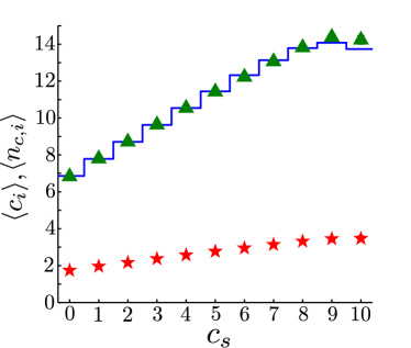
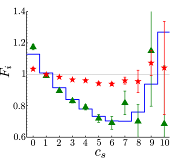
(a)                                                                    (b)

Figure 2: (a) Mean idler photocount number $\langle c_{\rm i}\rangle$ and photon number $\langle n_{\rm c,i}\rangle$ and (b) Fano factor $F_{\rm i}$ [$F_{\rm i}\equiv(\langle\hat{n}_{\rm i}^{2}\rangle-\langle\hat{n}_{\rm i}\rangle^{2})/\langle\hat{n}_{\rm i}\rangle$] as they depend on the signal photocount number $c_{\rm s}$. The values appropriate for the distributions of experimental photocounts are plotted with red asterisks whereas those characterizing the reconstructed photon-number distributions arising from the maximum-likelihood method (from the best fit of the twin beam) are plotted with green triangles (blue solid curves). Error bars in (a) are smaller than the used symbols.

The corresponding Fano factors $F_{\rm i}$ determined from the first- and second-order moments and drawn in Fig. 2(b) identify, within the experimental errors, the conditional fields with $c_{\rm s}\in<2,7>$ as sub-Poissonian. They also suggest that the nonclassicality of the conditional idler fields increases as $c_{\rm s}$ increases from 2 to 6, but then the nonclassicality decreases and it is lost for $c_{\rm s}=9$. This behavior originates in the noise present both in the experimental twin beam and the iCCD camera (that makes the postselection, smaller $c_{\rm s}$) as well as the relatively low detection efficiency of the iCCD camera (greater $c_{\rm s}$) [35].

Fano factors $F_{\rm i}$ for $c_{\rm s}>4$ plotted in Fig. 2(b) are determined with larger errors that increase with the increasing signal photocount number $c_{\rm s}$. This originates in relatively small numbers of measurements appropriate for the mentioned numbers $c_{\rm s}$. Mean numbers of these measurements are described by the signal-field photocount distribution $f_{\rm s}$ plotted in Fig. 3.

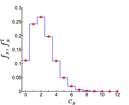
Figure 3: Marginal signal-field photocount distribution $f_{\rm s}(c_{\rm s})=\sum_{c_{\rm i}}f(c_{\rm s},c_{\rm i})$ (red asterisks) and its theoretical prediction $f^{\rm t}_{\rm s}$ defined below Eq. (23) (blue solid curve). Error bars of $f_{\rm s}$ are smaller than the used symbols.

According to this distribution, the probability of detecting the signal photocount numbers $c_{\rm s}$ greater than 7 is less than 1 %. Despite the large number $N=1.2\times 10^{6}$ of experimental repetitions, the determined quantities suffer from relatively large experimental errors in these cases. The experimental errors (for photocounts) are quantified by the mean squared fluctuation $\sigma_{x}$ ($\sigma_{x}=\sqrt{\langle x^{2}\rangle-\langle x\rangle^{2}}$) multiplied by factor $1/\sqrt{N_{\rm r}}$ that depends on the number $N_{\rm r}$ of actual experimental realizations. This approach was also applied to the determination of error bars of the quantities characterizing the photon-number distributions reached by the maximum-likelihood reconstruction. In this method that gives the most-probable photon-number distribution the experimental errors are naturally smoothed [also due to the form of $T_{a}$ given in Eq. (21) that includes $D_{a}$]. We note that the extended approach based on the Fischer information matrix [43] allows to quantify their contribution to the uncertainty characterizing the reconstructed photon-number distribution. The reconstruction based on the best fit of the 2D experimental histogram $f(c_{\rm s},c_{\rm i})$ exploits the whole ensemble of the measured data with $N=1.2\times 10^{6}$ entries and so the corresponding relative errors are negligible.

The nonclassicality identifiers $R$ belonging to the experimental photocounts and plotted in Fig. 4 identify the conditional idler fields with $c_{\rm s}\in<2,7>$ as nonclassical, in agreement with the predictions made by the Fano factors.

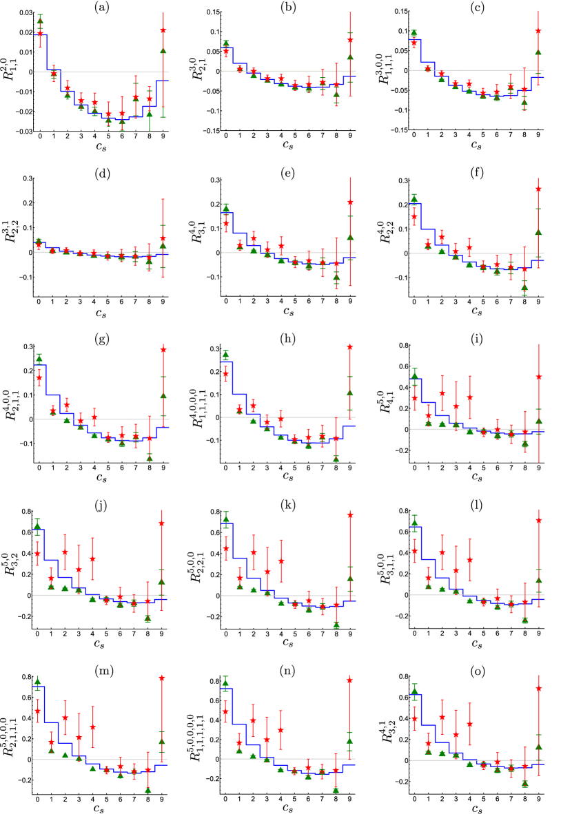
Figure 4: Nonclassicality identifiers $R$ given in Eqs. (11)—(13) and determined for distributions of experimental photocounts (red asterisks with error bars), photon-number distributions reached by the maximum-likelihood reconstruction method (green triangles with error bars) and photon-number distributions derived from the best fit of the twin beam (blue solid curves) as they depend on the signal photocount number $c_{\rm s}$. Some error bars are smaller than the plotted symbols.

According to the graphs in Fig. 4, nonclassical conditional idler fields can be divided into two groups. The conditional idler fields with $c_{\rm s}\in$ $<5,7>$ have all fifteen nonclassicality identifiers $R$ negative, determined both for photocounts and photon numbers. Such fields can thus be considered as firmly nonclassical. This accords with the lowest attained values of the Fano factor $F_{\rm i}(c_{\rm s})$ shown in Fig. 2(b). On the other hand, the conditional idler fields with $c_{\rm s}\in<2,4>$ have negative only the nonclassicality identifiers $R$ of the ’order’, given as the sum of their upper (or equivalently lower) indices, lower than four. The nonclassicality identifiers $R$ of ’order’ four and five are positive for the experimental photocounts. The maximum-likelihood reconstruction, that relies on the whole 1D experimental histograms, additionally provides negative nonclassicality identifiers $R$ of ’order’ four for $c_{\rm s}\in$ $<3,4>$ and five for $c_{\rm s}=4$. This corresponds to the decreasing values of Fano factor $F_{\rm i}(c_{\rm s})$ drawn in Fig. 2(b). Detailed inspection of the graphs in Fig. 4 reveals that the behavior of nonclassicality identifiers $R$ reached by the maximum-likelihood reconstruction qualitatively agrees (up to $c_{\rm s}=7$) with the behavior predicted by the reconstruction based on the best fit of the 2D experimental histogram and quantified by blue solid curves in the graphs of Figs. 2 and 4.

Compared to the Fano factor $F_{\rm i}$, the nonclassicality identifiers $R$ of ’order’ three or higher are endowed with weaker capability to reveal the nonclassicality of the analyzed states obtained by the post-selection method. The greater the ’order’ of nonclassicality identifier $R$ the weaker the capability. On the other hand, if the nonclassicality is observed in the nonclassicality identifiers $R$ of higher ’order’ it can be considered in certain sense as firm. This is the case of the conditional idler fields obtained after postselecting by the detection of 5, 6 and 7 signal photocounts. These fields, containing on average about 12-14 idler photons, exhibit their nonclassicality in all observed nonclassicality identifiers.

4 Conclusions

We have shown that the majorization theory provides a greater number and more suitable nonclassicality identifiers based on intensity moments compared to the commonly used matrix method. Considering the products of moments up to the fifth order, we identified fifteen independent identifiers and tested them on the experimental states with different ’degree’ of sub-Poissonian photon-number statistics. Identifiers based on lower intensity moments were identified as more powerful compared to those containing greater intensity moments. The latter ones have been found useful for identifying states being firmly nonclassical.

Funding

GA ČR (project P205/12/0382); MŠMT ČR (project LO1305); IGA UP Olomouc (project IGA_PrF_2016_002) - I. Arkhipov.

References

- [1] N. Bloembergen, Nonlinear Optics (W. A. Benjamin, 1965).
- [2] R. J. Glauber, Quantum Theory of Optical Coherence: Selected Papers and Lectures (Wiley-VCH, 2007).
- [3] R. J. Glauber, “Coherent and incoherent states of the radiation field,” Phys. Rev. 131, 2766—2788 (1963).
- [4] E. C. G. Sudarshan, “Equivalence of semiclassical and quantum mechanical descriptions of statistical light beams,” Phys. Rev. Lett. 10, 277 (1963).
- [5] L. Mandel and E. Wolf, Optical Coherence and Quantum Optics (Cambridge University, 1995).
- [6] A. I. Lvovsky and M. G. Raymer, “Continuous-variable optical quantum state tomography,” Rev. Mod. Phys. 81, 299 (2009).
- [7] E. Shchukin and W. Vogel, “Universal measurement of quantum correlations of radiation,” Phys. Rev. Lett. 96, 200403 (2006).
- [8] J. Peřina, Quantum Statistics of Linear and Nonlinear Optical Phenomena (Kluwer, 1991).
- [9] O. Haderka, J. Peřina Jr., M. Hamar, and J. Peřina, “Direct measurement and reconstruction of nonclassical features of twin beams generated in spontaneous parametric down-conversion,” Phys. Rev. A 71, 033815 (2005).
- [10] J. Peřina Jr., “Photocount measurements as a tool for investigation of non-classical properties of twin beams,” in “Wave and Quantum Aspects of Contemporary Optics,” vol. 7141 of SPIE Conference proceedings, A. Popiolek-Masajada, E. Jankowska, and W. Urbanczyk, eds. (SPIE, 2008), p. 714104.
- [11] J. Peřina Jr., M. Hamar, V. Michálek, and O. Haderka, “Photon-number distributions of twin beams generated in spontaneous parametric down-conversion and measured by an intensified CCD camera,” Phys. Rev. A 85, 023816 (2012).
- [12] J. Peřina Jr., O. Haderka, V. Michálek, and M. Hamar, “State reconstruction of a multimode twin beam using photodetection,” Phys. Rev. A 87, 022108 (2013).
- [13] I. I. Arkhipov and J. Peřina Jr., “Retrieving the covariance matrix of an unknown two-mode Gaussian state by means of a reference twin beam,” Opt. Commun. 375, 29—33 (2016).
- [14] J. K. Asbóth, J. Calsamiglia, and H. Ritsch, “Squeezing as an irreducible resource,” Phys. Rev. Lett. 94, 173602 (2005).
- [15] I. I. Arkhipov, J. Peřina Jr., J. Svozilík, and A. Miranowicz, “Nonclassicality invariant of general two-mode Gaussian states,” Sci. Rep. 6, 26523 (2016).
- [16] I. I. Arkhipov, J. Peřina Jr., J. Peřina, and A. Miranowicz, “Interplay of nonclassicality and entanglement of two-mode Gaussian fields generated in optical parametric processes,” Phys. Rev. A 94, 013807 (2016).
- [17] C. T. Lee, “Nonclassical photon statistics of two-mode squeezed states,” Phys. Rev. A 42, 1608—1616 (1990).
- [18] C. T. Lee, “General criteria for nonclassical photon statistics in multimode radiations,” Opt. Lett. 15, 1386—1388 (1990).
- [19] A. Verma and A. Pathak, “Generalized structure of higher-order nonclassicality,” Phys. Lett. A 374, 1009 (2010).
- [20] J. Sperling, W. Vogel, and G. S. Agarwal, “Sub-binomial light,” Phys. Rev. Lett. 109, 093601 (2012).
- [21] S. K. Giri, B. Sen, C. H. R. Ooi, and A. Pathak, “Single-mode and intermodal higher-order nonclassicalities in two-mode Bose-Einstein condensates,” Phys. Rev. A 89, 033628 (2014).
- [22] R. Short and L. Mandel, “Observation of sub-Poissonian photon statistics,” Phys. Rev. Lett. 51, 384—387 (1983).
- [23] M. Avenhaus, K. Laiho, M. V. Chekhova, and C. Silberhorn, “Accessing higher-order correlations in quantum optical states by time multiplexing,” Phys. Rev. Lett. 104, 063602 (2010).
- [24] A. Allevi, S. Olivares, and M. Bondani, “Photon-number correlations by photon-number resolving detectors,” Phys. Rev. A 85, 063835 (2012).
- [25] J. Sperling, M. Bohmann, W. Vogel, G. Harder, B. Brecht, V. Ansari, and C. Silberhorn, “Uncovering quantum correlations with time-multiplexed click detection,” Phys. Rev. Lett. 115, 023601 (2015).
- [26] G. Agarwal and K. Tara, “Nonclassical character of states exhibiting no squeezing or sub-Poissonian statistics,” Phys. Rev. A 46, 485—488 (1992).
- [27] E. Shchukin, T. Richter, and W. Vogel, “Nonclassicality criteria in terms of moments,” Phys. Rev. A 71, 011802(R) (2005).
- [28] W. Vogel, “Nonclassical correlation properties of radiation fields,” Phys. Rev. Lett. 100, 013605 (2008).
- [29] A. Miranowicz, M. Bartkowiak, X. Wang, X.-Y. Liu, and F. Nori, “Testing nonclassicality in multimode fields: A unified derivation of classical inequalities,” Phys. Rev. A 82, 013824 (2010).
- [30] T. Richter and W. Vogel, “Nonclassicality of quantum states: A hierarchy of observable conditions,” Phys. Rev. Lett. 89, 283601 (2002).
- [31] S. Ryl, J. Sperling, E. Agudelo, M. Mraz, S. Köhnke, B. Hage, and W. Vogel, “Unified nonclassicality criteria,” Phys. Rev. A 92, 011801(R) (2015).
- [32] A. W. Marshall, I. Olkin, and B. C. Arnold, Inequalities: Theory of Majorization and its Application, 2nd ed. (Springer, 2010).
- [33] C. T. Lee, “Higher-order criteria for nonclassical effects in photon statistics,” Phys. Rev. A 41, 1721—1723 (1990).
- [34] A. Allevi, M. Bondani, and A. Andreoni, “Photon-number correlations by photon-number resolving detectors,” Opt. Lett. 35, 1707–1709 (2010).
- [35] J. Peřina Jr., O. Haderka, and V. Michálek, “Sub-Poissonian-light generation by postselection from twin beams,” Opt. Express 21, 19387—19394 (2013).
- [36] I. I. Arkhipov, J. Peřina Jr., J. Peřina, and A. Miranowicz, “Comparative study of nonclassicality, entanglement, and dimensionality of multimode noisy twin beams,” Phys. Rev. A 91, 033837 (2015).
- [37] J. Laurat, T. Coudreau, N. Treps, A. Maitre, and C. Fabre, “Conditional preparation of a quantum state in the continuous variable regime: Generation of a sub-Poissonian state from twin beams,” Phys. Rev. Lett. 91, 213601 (2003).
- [38] M. Lamperti, A. Allevi, M. Bondani, R. Machulka, V. Michálek, O. Haderka, and J. Peřina Jr., “Optimal sub-Poissonian light generation from twin beams by photon-number resolving detectors,” J. Opt. Soc. Am. B 31, 20–25 (2014).
- [39] M. Hamar, J. Peřina Jr., O. Haderka, and V. Michálek, “Transverse coherence of photon pairs generated in spontaneous parametric down-conversion,” Phys. Rev. A 81, 043827 (2010).
- [40] A. P. Dempster, N. M. Laird, and D. B. Rubin, “Maximum likelihood from incomplete data via the EM algorithm,” J. R. Statist. Soc. B 39, 1—38 (1977).
- [41] J. Peřina Jr., O. Haderka, M. Hamar, and V. Michálek, “Absolute detector calibration using twin beams,” Opt. Lett. 37, 2475—2477 (2012).
- [42] J. Peřina and J. Křepelka, “Multimode description of spontaneous parametric down-conversion,” J. Opt. B: Quant. Semiclass. Opt. 7, 246—252 (2005).
- [43] B. R. Frieden, Science from Fisher Information: A Unification (Cambridge University, 2004).