On the Convergence of Asynchronous Parallel Iteration with Unbounded Delays

Abstract

Recent years have witnessed the surge of asynchronous parallel (async-parallel) iterative algorithms due to problems involving very large-scale data and a large number of decision variables. Because of asynchrony, the iterates are computed with outdated information, and the age of the outdated information, which we call delay, is the number of times it has been updated since its creation. Almost all recent works prove convergence under the assumption of a finite maximum delay and set their stepsize parameters accordingly. However, the maximum delay is practically unknown.

This paper presents convergence analysis of an async-parallel method from a probabilistic viewpoint, and it allows for large unbounded delays. An explicit formula of stepsize that guarantees convergence is given depending on delays’ statistics. With $p+1$ identical processors, we empirically measured that delays closely follow the Poisson distribution with parameter $p$, matching our theoretical model, and thus the stepsize can be set accordingly. Simulations on both convex and nonconvex optimization problems demonstrate the validness of our analysis and also show that the existing maximum-delay induced stepsize is too conservative, often slowing down the convergence of the algorithm.

1 Introduction

In the “big data” era, the size of the dataset and the number of decision variables involved in many areas such as health care, the Internet, economics, and engineering are becoming tremendously large WH2014big . It motivates the development of new computational approaches by efficiently utilizing modern multi-core computers or computing clusters.

In this paper, we consider the block-structured optimization problem

$$\operatorname*{minimize}_{{\mathbf{x}}\in\mathbb{R}^{n}}F({\mathbf{x}})\equiv f({\mathbf{x}}_{1},\ldots,{\mathbf{x}}_{m})+\sum_{i=1}^{m}r_{i}({\mathbf{x}}_{i}),$$ (1)

where ${\mathbf{x}}=({\mathbf{x}}_{1},\ldots,{\mathbf{x}}_{m})$ is partitioned into $m$ disjoint blocks, $f$ has a Lipschitz continuous gradient (possibly nonconvex), and $r_{i}$’s are (possibly nondifferentiable) proper closed convex functions. Note that $r_{i}$’s can be extended-valued, and thus (1) can have block constraints ${\mathbf{x}}_{i}\in X_{i}$ by incorporating the indicator function of $X_{i}$ in $r_{i}$ for all $i$.

Many applications can be formulated in the form of (1), and they include classic machine learning problems: support vector machine (squared hinge loss and its dual formulation) cortes1995-SVM , LASSO tibshirani1996-Lasso , and logistic regression (linear or multilinear) zhou2013tensor-reg , and also subspace learning problems: sparse principal component analysis zou2006sparse-PCA , nonnegative matrix or tensor factorization cichocki2009NMF-NTF , just to name a few.

Toward solutions for these problems with extremely large-scale datasets and many variables, first-order methods and also stochastic methods become particularly popular because of their scalability to the problem size, such as FISTA beck2009FISTA , stochastic approximation nemirovski2009robust , randomized coordinate descent nesterov2012RCD , and their combinations DangLan-SBMD ; XuYin2015_block . Recently, lots of efforts have been made to the parallelization of these methods, and in particular, asynchronous parallel (async-parallel) methods attract more attention (e.g., liu2014asynchronous ; Peng_2015_AROCK ) over their synchronous counterparts partly due to the better speed-up performance.

This paper focuses on the async-parallel block coordinate update (async-BCU) method (see Algorithm 1) for solving (1). To the best of our knowledge, all works on async-BCU before 2013 consider a deterministic selection of blocks with an exception to Strikwerda2002125 , and thus they require strong conditions (like a contraction) for convergence. Recent works, e.g., liu2014asynchronous ; liu2015async-scd ; Peng_2015_AROCK ; hannah2016unbounded , employ randomized block selection and significantly weaken the convergence requirement. However, all of them require bounded delays and/or are restricted to convex problems. The work hannah2016unbounded allows unbounded delays but requires convexity, and davis2016asynchronous ; cannelli2016asynchronous do not assume convexity but require bounded delays. We consider unbounded delays and deal with nonconvex problems.

1.1 Algorithm

We describe the async-BCU method as follows. Assume there are $p+1$ processors, and the data and variable ${\mathbf{x}}$ are accessible to all processors. We let all processors continuously and asynchronously update the variable ${\mathbf{x}}$ in parallel. At each time $k$, one processor reads the variable ${\mathbf{x}}$ as $\hat{{\mathbf{x}}}^{k}$ from the global memory, randomly picks a block $i_{k}\in\{1,2,\cdots,m\}$, and renews ${\mathbf{x}}_{i_{k}}$ by a prox-linear update while keeping all the other blocks unchanged. The pseudocode is summarized in Algorithm 1, where the ${\mathbf{prox}}$ operator is defined in (3).

The algorithm first appeared in liu2014asynchronous , where the age of $\hat{{\mathbf{x}}}^{k}$ relative to ${\mathbf{x}}^{k}$, which we call the delay of iteration $k$, was assumed to be bounded by a certain integer $\tau$. For general convex problems, sublinear convergence was established, and for the strongly convex case, linear convergence was shown. However, its convergence for nonconvex problems and/or with unbounded delays was unknown. In addition, numerically, the stepsize is difficult to tune because it depends on $\tau$, which is unknown before the algorithm completes.

Input : Any point ${\mathbf{x}}^{0}\in\mathbb{R}^{n}$ in the global memory, maximum number of iterations $K$, stepsize $\eta>0$

while $k<K$, each and all processors asynchronously do

       select $i_{k}$ from $[m]$ uniformly at random; 

      $\hat{{\mathbf{x}}}^{k}\leftarrow$ read ${\mathbf{x}}$ from the global memory; 

      for all $i\in[m],$ 

$${\mathbf{x}}^{k+1}_{i}\leftarrow\begin{cases}{\mathbf{prox}}_{\eta r_{i}}\left({\mathbf{x}}_{i}^{k}-\eta\nabla_{i}f(\hat{{\mathbf{x}}}^{k})\right),&\text{ if }i=i_{k},\\ {\mathbf{x}}_{i}^{k},&\text{ otherwise};\end{cases}$$ (2)

increase the global counter $k\leftarrow k+1$; 

end while

Algorithm 1 Async-parallel block coordinate update

1.2 Contributions

We summarize our contributions as follows.

• We analyze the convergence of Algorithm 1 and allow for large unbounded delays following a certain distribution. We require the delays to have certain bounded expected quantities (e.g., expected delay, variance of delay). Our results are more general than those requiring bounded delays such as liu2014asynchronous ; liu2015async-scd .

• Both nonconvex and convex problems are analyzed, and those problems include both smooth and nonsmooth functions. For nonconvex problems, we establish the global convergence in terms of first-order optimality conditions and show that any limit point of the iterates is a critical point almost surely. It appears to be the first result of an async-BCU method for general nonconvex problems and allowing unbounded delays. For weakly convex problems, we establish a sublinear convergence result, and for strongly convex problems, we show the linear convergence.

• We show that if all $p+1$ processors run at the same speed, the delay follows the Poisson distribution with parameter $p$. In this case, all the relevant expected quantities can be explicitly computed and are bounded. By setting appropriate stepsizes, we can reach a near-linear speedup if $p=o(\sqrt{m})$ for smooth cases and $p=o(\sqrt[4]{m})$ for nonsmooth cases.

• When the delay follows the Poisson distribution, we can explicitly set the stepsize based on the delay expectation (which equals $p$). We simulate the async-BCU method on one convex problem: LASSO, and one nonconvex problem: the nonnegative matrix factorization. The results demonstrate that async-BCU performs consistently better with a stepsize set based on the expected delay than on the maximum delay. The number of processors is known while the maximum delay is not. Hence, the setting based on expected delay is practically more useful.

Our algorithm updates one (block) coordinate of ${\mathbf{x}}$ in each step and is sharply different from stochastic gradient methods that sample one function in each step to update all coordinates of ${\mathbf{x}}$. While there are async-parallel algorithms in either classes and how to handle delays is important to both of their convergence, their basic lines of analysis are different with respect to how to absorb the delay-induced errors. The results of the two classes are in general not comparable. That said, for problems with certain proper structures, it is possible to apply both coordinate-wise update and stochastic sampling (e.g., recht2011hogwild ; XuYin2015_block ; MokhtaiKoppelRibeiro2016_class ; davis2016asynchronous ), and our results apply to the coordinate part.

1.3 Notation and assumptions

Throughout the paper, bold lowercase letters ${\mathbf{x}},{\mathbf{y}},\ldots,$ are used for vectors. We denote ${\mathbf{x}}_{i}$ as the $i$-th block of ${\mathbf{x}}$ and $U_{i}$ as the $i$-th sampling matrix, i.e., $U_{i}{\mathbf{x}}$ is a vector with ${\mathbf{x}}_{i}$ as its $i$-th block and $\mathbf{0}$ for the remaining ones. $\mathbb{E}_{i_{k}}$ denotes the expectation with respect to $i_{k}$ conditionally on all previous history, and $[m]=\{1,\ldots,m\}$.

We consider the Euclidean norm denoted by $\|\cdot\|$, but all our results can be directly extended to problems with general primal and dual norms in a Hilbert space.

The projection to a convex set $X$ is defined as

$$\textstyle{\mathcal{P}}_{X}({\mathbf{y}})=\operatorname*{arg\,min}\limits_{{\mathbf{x}}\in X}\|{\mathbf{x}}-{\mathbf{y}}\|^{2},$$

and the proximal mapping of a convex function $h$ is defined as

$$\textstyle{\mathbf{prox}}_{h}({\mathbf{y}})=\operatorname*{arg\,min}\limits_{\mathbf{x}}h({\mathbf{x}})+\tfrac{1}{2}\|{\mathbf{x}}-{\mathbf{y}}\|^{2}.$$ (3)

Definition 1

(Critical point) A point ${\mathbf{x}}^{*}$ is a critical point of (1) if $\mathbf{0}\in\nabla f({\mathbf{x}}^{*})+\partial R({\mathbf{x}}^{*}),$ where $\partial R({\mathbf{x}})$ denotes the subdifferential of $R$ at ${\mathbf{x}}$ and

$$R({\mathbf{x}})=\sum_{i=1}^{m}r_{i}({\mathbf{x}}_{i}).$$ (4)

Throughout our analysis, we make the following three assumptions to problem (1) and Algorithm 1. Other assumed conditions will be specified if needed.

Assumption 1

The function $F$ is lower bounded. The problem (1) has at least one solution, and the solution set is denoted as $X^{*}$.

Assumption 2

$\nabla f({\mathbf{x}})$ is Lipschitz continuous with constant $L_{f}$, namely,

$$\|\nabla f({\mathbf{x}})-\nabla f({\mathbf{y}})\|\leq L_{f}\|{\mathbf{x}}-{\mathbf{y}}\|,\,\forall{\mathbf{x}},~{}{\mathbf{y}}.$$ (5)

In addition, for each $i\in[m]$, fixing all block coordinates but the $i$-th one, $\nabla f({\mathbf{x}})$ and $\nabla_{i}f({\mathbf{x}})$ are Lipschitz continuous about ${\mathbf{x}}_{i}$ with $L_{r}$ and $L_{c}$, respectively, i.e., for any ${\mathbf{x}},~{}{\mathbf{y}}$, and $i$,

$$\|\nabla f({\mathbf{x}})-\nabla f({\mathbf{x}}+U_{i}{\mathbf{y}})\|\leq L_{r}\|{\mathbf{y}}_{i}\|,$$ (6)

$$\|\nabla_{i}f({\mathbf{x}})-\nabla_{i}f({\mathbf{x}}+U_{i}{\mathbf{y}})\|\leq L_{c}\|{\mathbf{y}}_{i}\|.$$ (7)

From (7), we have that for any ${\mathbf{x}},~{}{\mathbf{y}}$, and $i$,

$$f({\mathbf{x}}+U_{i}{\mathbf{y}})\leq f({\mathbf{x}})+\langle\nabla_{i}f({\mathbf{x}}),{\mathbf{y}}_{i}\rangle+\tfrac{L_{c}}{2}\|{\mathbf{y}}_{i}\|^{2}.$$ (8)

We denote $\kappa=\frac{L_{r}}{L_{c}}$ as the condition number.

Assumption 3

For each $k\geq 1$, the reading $\hat{{\mathbf{x}}}^{k}$ is consistent and delayed by $j_{k}$, namely, $\hat{{\mathbf{x}}}^{k}={\mathbf{x}}^{k-j_{k}}$. The delay $j_{k}$ follows an identical distribution as a random variable ${\mathbf{j}}$

$${\mathrm{Prob}}({\mathbf{j}}=t)=q_{t},\,t=0,1,2\ldots,$$ (9)

and is independent of $i_{k}$. We let

$$\textstyle c_{k}:=\sum_{t=k}^{\infty}q_{t},\qquad T:=\mathbb{E}[{\mathbf{j}}],\qquad S:=\mathbb{E}[{\mathbf{j}}^{2}].$$

Remark 1

Although the delay always satisfies $0\leq j_{k}\leq k$, the assumption in (9) is without loss of generality if we make negative iterates and regard ${\mathbf{x}}^{k}={\mathbf{x}}^{0},\,\forall k<0$. For simplicity, we make the identical distribution assumption, which is the same as that in Strikwerda2002125 . Our results can still hold for non-identical distribution; see the analysis for the smooth nonconvex case in the arXiv version of the paper.

2 Related works

We briefly review block coordinate update (BCU) and async-parallel computing methods.

The BCU method is closely related to the Gauss-Seidel method for solving linear equations, which can date back to 1823. In the literature of optimization, BCU method first appeared in Hildreth-57 as the block coordinate descent method, or more precisely, block minimization (BM), for quadratic programming. The convergence of BM was established early for both convex and nonconvex problems, for example luo1992convergence ; Grippo-Sciandrone-00 ; Tseng-01 . However, in general, its convergence rate result was only shown for strongly convex problems (e.g., luo1992convergence ) until the recent work hong2015iteration that shows sublinear convergence for weakly convex cases. tseng2009_CGD proposed a new version of BCU methods, called coordinate gradient descent method, which mimics proximal gradient descent but only updates a block coordinate every time. The block coordinate gradient or block prox-linear update (BPU) becomes popular since nesterov2012RCD proposed to randomly select a block to update. The convergence rate of the randomized BPU is easier to show than the deterministic BPU. It was firstly established for convex smooth problems (both unconstrained and constrained) in nesterov2012RCD and then generalized to nonsmooth cases in richtarik2014iteration ; Lu_Xiao_rbcd_2015 . Recently, DangLan-SBMD ; XuYin2015_block incorporated stochastic approximation into the BPU framework to deal with stochastic programming, and both established sublinear convergence for convex problems and also global convergence for nonconvex problems.

The async-parallel computing method (also called chaotic relaxation) first appeared in rosenfeld1969case to solve linear equations arising in electrical network problems. D-W1969chaotic-relax first systematically analyzed (more general) asynchronous iterative methods for solving linear systems. Assuming bounded delays, it gave a necessary and sufficient condition for convergence. bertsekas1983distributed proposed an asynchronous distributed iterative method for solving more general fixed-point problems and showed its convergence under a contraction assumption. TB1990partially weakened the contraction assumption to pseudo-nonexpansiveness but made more other assumptions. FS2000asyn-review made a thorough review of asynchronous methods before 2000. It summarized convergence results under nested sets and synchronous convergence conditions, which are satisfied by P-contraction mappings and isotone mappings.

Since it was proposed in 1969, the async-parallel method has not attracted much attention until recent years when the size of data is increasing exponentially in many areas. Motivated by “big data” problems, liu2014asynchronous ; liu2015async-scd proposed the async-parallel stochastic coordinate descent method (i.e., Algorithm 1) for solving problems in the form of (1). Their analysis focuses on convex problems and assumes bounded delays. Specifically, they established sublinear convergence for weakly convex problems and linear convergence for strongly convex problems. In addition, near-linear speed up was achieved if $\tau=o(\sqrt{m})$ for unconstrained smooth convex problems and $\tau=o(\sqrt[4]{m})$ for constrained smooth or nonsmooth cases. For nonconvex problems, davis2016asynchronous introduced an async-parallel coordinate descent method, whose convergence was established under iterate boundedness assumptions and appropriate stepsizes.

3 Convergence results for the smooth case

Throughout this section, let $r_{i}=0,\,\forall i$, i.e., we consider the smooth optimization problem

$$\textstyle\operatorname*{minimize}\limits_{{\mathbf{x}}\in\mathbb{R}^{n}}f({\mathbf{x}}).$$ (10)

The general (possibly nonsmooth) case will be analyzed in the next section. The results for nonsmooth problems of course also hold for smooth ones. However, the smooth case requires weaker conditions for convergence than those required by the nonsmooth case, and their analysis techniques are different. Hence, we consider the two cases separately.

3.1 Convergence for the nonconvex case

In this subsection, we establish a subsequence convergence result for the general (possibly nonconvex) case. We begin with some technical lemmas. The first lemma deals with certain infinite sums that will appear later in our analysis.

Lemma 1

For any $k$ and $t\leq k$, let

$$\textstyle\gamma_{k}=\frac{\eta^{2}L_{r}}{2m\sqrt{m}}\sum_{d=1}^{k-1}(c_{k-d}-c_{k})c_{d}+\frac{\eta}{2m}c_{k}+\frac{\eta^{2}L_{c}}{2m}c_{k},$$ (11a)

$$\textstyle\beta_{k}=\left(\frac{\eta}{m}-\frac{\eta^{2}L_{c}}{2m}\right)q_{0}-\frac{\eta}{2m}c_{k}\textnormal{ for }k\geq 1,~{}~{}\left(\textnormal{and }\beta_{0}=0\right),$$ (11b)

$$\textstyle C_{t,k}=\left(\frac{\eta}{m}-\frac{\eta^{2}L_{c}}{2m}\right)q_{t}-\frac{\eta^{2}L_{r}}{2m\sqrt{m}}\left(tq_{t}+\sum_{d=1}^{t}(c_{d}-c_{k})q_{t-d}\right).$$ (11c)

Then

$$\textstyle\sum_{k=0}^{\infty}\gamma_{k}\leq{\tfrac{\eta^{2}L_{r}}{2m\sqrt{m}}}T^{2}+\left(\frac{\eta}{2m}+\frac{\eta^{2}L_{c}}{2m}\right)(1+T),$$ (12)

$$\textstyle\beta_{k}+\sum_{t=k+1}^{\infty}C_{t-k,t}\geq\frac{\eta}{2m}-\frac{\eta^{2}L_{c}}{2m}-\frac{\eta^{2}L_{r}T}{m\sqrt{m}},\,\forall k.$$ (13)

Proof

To bound $\sum_{k=0}^{\infty}\gamma_{k}$, we bound the first term $\sum_{d=1}^{k-1}(c_{k-d}-c_{k})c_{d}$ in (11a). Specifically,

$$\sum_{k=0}^{\infty}\sum_{d=1}^{k-1}(c_{k-d}-c_{k})c_{d}\leq\sum_{k=0}^{\infty}\sum_{d=1}^{k-1}c_{k-d}c_{d}=\sum_{d=1}^{\infty}\sum_{k=d+1}^{\infty}c_{k-d}c_{d}=T^{2},$$

where the last equality holds since $T:=\mathbb{E}[{\mathbf{j}}]=\sum_{t=1}^{\infty}tq_{t}=\sum_{t=1}^{\infty}\sum_{d=1}^{t}q_{t}=\sum_{d=1}^{\infty}\sum_{t=d}^{\infty}q_{t}=\sum_{d=1}^{\infty}c_{d}.$ We obtain (12) by combining these two equations.

To prove (13), we will use

$$\textstyle\sum\limits_{t=1}^{\infty}\sum\limits_{d=1}^{t}(c_{d}-c_{k+t})q_{t-d}\leq\sum\limits_{t=1}^{\infty}\sum\limits_{d=1}^{t}c_{d}q_{t-d}=\sum\limits_{d=1}^{\infty}\sum\limits_{t=d}^{\infty}c_{d}q_{t-d}=\sum\limits_{d=1}^{\infty}c_{d}=T.$$ (14)

The above inequality yields

$$\textstyle\beta_{k}+\sum_{t=k+1}^{\infty}C_{t-k,t}=\beta_{k}+\sum_{t=1}^{\infty}C_{t,t+k}$$

$$= \textstyle\big{(}\frac{\eta}{m}-\frac{\eta^{2}L_{c}}{2m}\big{)}q_{0}-\frac{\eta}{2m}c_{k}$$

$$\textstyle+\sum_{t=1}^{\infty}\Big{(}\big{(}\frac{\eta}{m}-\frac{\eta^{2}L_{c}}{2m}\big{)}q_{t}-\frac{\eta^{2}L_{r}}{2m\sqrt{m}}tq_{t}-\frac{\eta^{2}L_{r}}{2m\sqrt{m}}\sum_{d=1}^{t}(c_{d}-c_{k+t})q_{t-d}\Big{)}$$

$$\stackrel{{\scriptstyle(\ref{ineq-cd})}}{{\geq}} \textstyle\frac{\eta}{m}-\frac{\eta^{2}L_{c}}{2m}-\frac{\eta}{2m}c_{k}-\frac{\eta^{2}L_{r}T}{m\sqrt{m}}\geq\frac{\eta}{2m}-\frac{\eta^{2}L_{c}}{2m}-\frac{\eta^{2}L_{r}T}{m\sqrt{m}},$$

where the last inequality follows from $c_{k}\leq 1$. ∎

The second lemma below bounds the cross term that appears in our analysis.

Lemma 2 (Cross term bound)

For any $k>1$ and $t\leq k$, it holds that

$$\textstyle\sum_{t=1}^{k-1}q_{t}\mathbb{E}\Big{[}-\langle\nabla f({\mathbf{x}}^{k})-\nabla f({\mathbf{x}}^{k-t}),\nabla f({\mathbf{x}}^{k-t})\rangle\Big{]}$$ (15)

$$\leq \textstyle\frac{\eta L_{r}}{2\sqrt{m}}\sum_{t=1}^{k-1}\left(tq_{t}+\sum\limits_{d=1}^{t}(c_{d}-c_{k})q_{t-d}\right)\mathbb{E}\|\nabla f({\mathbf{x}}^{k-t})\|^{2}$$ (16)

$$+\textstyle\frac{\eta L_{r}}{2\sqrt{m}}\sum_{d=1}^{k-1}(c_{k-d}-c_{k})c_{d}\|\nabla f({\mathbf{x}}^{0})\|^{2}.$$

Proof

Define $\Delta^{d}:=\nabla f({\mathbf{x}}^{d})-\nabla f({\mathbf{x}}^{d+1})$. Applying the Cauchy-Schwarz inequality with $\nabla f({\mathbf{x}}^{k-t})-\nabla f({\mathbf{x}}^{k})=\sum_{d=k-t}^{k-1}\Delta^{d}$ yields

$$\textstyle-\langle\nabla f({\mathbf{x}}^{k})-\nabla f({\mathbf{x}}^{k-t}),\nabla f({\mathbf{x}}^{k-t})\rangle\leq\sum_{d=k-t}^{k-1}\|\Delta^{d}\|\cdot\|\nabla f({\mathbf{x}}^{k-t})\|.$$

Since $\|\Delta^{d}\|\leq L_{r}\|{\mathbf{x}}^{d+1}-{\mathbf{x}}^{d}\|=\eta L_{r}\|\nabla_{i_{d}}f({\hat{{\mathbf{x}}}}^{d})\|,$ by applying Young’s inequality, we get

$$-\langle\nabla f({\mathbf{x}}^{k})-\nabla f({\mathbf{x}}^{k-t}),\nabla f({\mathbf{x}}^{k-t})\rangle$$ (17)

$$\leq \textstyle\frac{\eta L_{r}}{2}\sum_{d=k-t}^{k-1}\Big{(}\sqrt{m}\|\nabla_{i_{d}}f({\hat{{\mathbf{x}}}}^{d})\|^{2}+\frac{1}{\sqrt{m}}\|\nabla f({\mathbf{x}}^{k-t})\|^{2}\Big{)}.$$ (18)

By taking expectation, we have

$$\mathbb{E}_{i_{d},j_{d}}\|\nabla_{i_{d}}f({\hat{{\mathbf{x}}}}^{d})\|^{2}= \textstyle\frac{1}{m}\mathbb{E}_{j_{d}}\|\nabla f({\mathbf{x}}^{d-j_{d}})\|^{2}$$

$$= \textstyle\frac{1}{m}\Big{(}\sum_{r=0}^{d-1}q_{r}\|\nabla f({\mathbf{x}}^{d-r})\|^{2}+c_{d}\|\nabla f({\mathbf{x}}^{0})\|^{2}\Big{)}.$$

Now taking expectation on both sides of (17) and using the above equation, we get

$$\mathbb{E}[-\langle\nabla f({\mathbf{x}}^{k})-\nabla f({\mathbf{x}}^{k-t}),\nabla f({\mathbf{x}}^{k-t})\rangle]$$ (19)

$$\leq \textstyle\frac{\eta L_{r}}{2\sqrt{m}}\sum_{d=k-t}^{k-1}\Big{(}\sum_{r=0}^{d-1}q_{r}\mathbb{E}\|\nabla f({\mathbf{x}}^{d-r})\|^{2}+c_{d}\|\nabla f({\mathbf{x}}^{0})\|^{2}\Big{)}$$ (20)

$$+\textstyle\frac{\eta L_{r}}{2\sqrt{m}}\sum_{d=k-t}^{k-1}t\mathbb{E}\|\nabla f({\mathbf{x}}^{k-t})\|^{2}.$$ (21)

Finally, (15) follows from

$$\textstyle\sum_{t=1}^{k-1}q_{t}\sum_{d=k-t}^{k-1}c_{d}\|\nabla f({\mathbf{x}}^{0})\|^{2}\overset{(\ref{seq1})}{=} \textstyle\sum_{d=1}^{k-1}\Big{(}\sum_{t=k-d}^{k-1}q_{t}\Big{)}c_{d}\|\nabla f({\mathbf{x}}^{0})\|^{2}$$

$$= \textstyle\sum_{d=1}^{k-1}(c_{k-d}-c_{k})c_{d}\|\nabla f({\mathbf{x}}^{0})\|^{2},$$

and

$$\textstyle\sum\limits_{t=1}^{k-1}q_{t}\sum\limits_{d=k-t}^{k-1}\sum\limits_{r=0}^{d-1}q_{r}\mathbb{E}\|\nabla f({\mathbf{x}}^{d-r})\|^{2}$$ (22)

$$= \textstyle\sum\limits_{d=1}^{k-1}(c_{k-d}-c_{k})\sum\limits_{r=0}^{d-1}q_{r}\mathbb{E}\|\nabla f({\mathbf{x}}^{d-r})\|^{2}$$ (23)

$$[\text{let }r\leftarrow d-r]~{}= \textstyle\sum\limits_{d=1}^{k-1}(c_{k-d}-c_{k})\sum\limits_{r=1}^{d}q_{d-r}\mathbb{E}\|\nabla f({\mathbf{x}}^{r})\|^{2}$$ (24)

$$\overset{(\ref{seq2})}{=} \textstyle\sum\limits_{r=1}^{k-1}\left(\sum\limits_{d=r}^{k-1}(c_{k-d}-c_{k})q_{d-r}\right)\mathbb{E}\|\nabla f({\mathbf{x}}^{r})\|^{2}$$ (25)

$$[\text{let }t\leftarrow k-r,\ d\leftarrow k-d]~{}= \textstyle\sum\limits_{t=1}^{k-1}\left(\sum\limits_{d=1}^{t}(c_{d}-c_{k})q_{t-d}\right)\mathbb{E}\|\nabla f({\mathbf{x}}^{k-t})\|^{2}.$$ (26)

∎

Using the above lemma, we show a result of running one iteration of the algorithm.

Theorem 3.1 (Fundamental bound)

Set $\gamma_{k},\beta_{k}$ and $C_{t,k}$ as in (11). For any $k>1$, we have

$$\textstyle\mathbb{E}f({\mathbf{x}}^{k+1})\leq \mathbb{E}f({\mathbf{x}}^{k})+\gamma_{k}\|\nabla f({\mathbf{x}}^{0})\|^{2}-\beta_{k}\mathbb{E}\|\nabla f({\mathbf{x}}^{k})\|^{2}$$ (27)

$$\textstyle-\sum_{t=1}^{k-1}C_{t,k}\mathbb{E}\|\nabla f({\mathbf{x}}^{k-t})\|^{2}.$$ (28)

Proof

Since ${\mathbf{x}}^{k+1}={\mathbf{x}}^{k}-\eta U_{i_{k}}\nabla f({\mathbf{x}}^{k-j_{k}})$, we have from (8) that

$$f({\mathbf{x}}^{k+1})\leq f({\mathbf{x}}^{k})-\eta\langle\nabla f({\mathbf{x}}^{k}),U_{i_{k}}\nabla f({\mathbf{x}}^{k-j_{k}})\rangle+\tfrac{L_{c}}{2}\|\eta U_{i_{k}}\nabla f({\mathbf{x}}^{k-j_{k}})\|^{2}.$$

Taking conditional expectation on $(i_{k},j_{k})$ gives

$$\mathbb{E}_{i_{k},j_{k}}f({\mathbf{x}}^{k+1})$$ (29)

$$\leq f({\mathbf{x}}^{k})-\tfrac{\eta}{m}\mathbb{E}_{j_{k}}\langle\nabla f({\mathbf{x}}^{k}),\nabla f({\mathbf{x}}^{k-j_{k}})\rangle+\tfrac{\eta^{2}L_{c}}{2m}\mathbb{E}_{j_{k}}\|\nabla f({\mathbf{x}}^{k-j_{k}})\|^{2}$$ (30)

$$= \textstyle f({\mathbf{x}}^{k})-\tfrac{\eta}{m}\sum_{t=0}^{k-1}q_{t}\langle\nabla f({\mathbf{x}}^{k}),\nabla f({\mathbf{x}}^{k-t})\rangle-\tfrac{\eta}{m}c_{k}\langle\nabla f({\mathbf{x}}^{k}),\nabla f({\mathbf{x}}^{0})\rangle$$ (31)

$$\textstyle+\tfrac{\eta^{2}L_{c}}{2m}\sum_{t=0}^{k-1}q_{t}\|\nabla f({\mathbf{x}}^{k-t})\|^{2}+\tfrac{\eta^{2}L_{c}}{2m}c_{k}\|\nabla f({\mathbf{x}}^{0})\|^{2}.$$ (32)

For the first cross term in (29), we write each summand as

$$\langle\nabla f({\mathbf{x}}^{k}),\nabla f({\mathbf{x}}^{k-t})\rangle=\langle\nabla f({\mathbf{x}}^{k})-\nabla f({\mathbf{x}}^{k-t}),\nabla f({\mathbf{x}}^{k-t})\rangle+\|\nabla f({\mathbf{x}}^{k-t})\|^{2},$$ (33)

and we use Young’s inequality to bound the second cross term by

$$-\tfrac{\eta}{m}c_{k}\langle\nabla f({\mathbf{x}}^{k}),\nabla f({\mathbf{x}}^{0})\rangle\leq\tfrac{\eta c_{k}}{2m}\Big{[}\|\nabla f({\mathbf{x}}^{k})\|^{2}+\|\nabla f({\mathbf{x}}^{0})\|^{2}\Big{]}.$$ (34)

Now taking expectation over both sides of (29), plugging in (33) and (34), and using Lemma 2, we have the desired result. ∎

We are now ready to show the main result in the following theorem.

Theorem 3.2

(Convergence for the nonconvex smooth case) Under Assumptions 1 through 3, let $\{{\mathbf{x}}^{k}\}_{k\geq 1}$ be generated from Algorithm 1. Assume $T<\infty$. Take the stepsize as $0<\eta<\frac{1/L_{c}}{1+2\kappa T/\sqrt{m}}.$ If $q_{0}>0$ or $\nabla f({\mathbf{x}})$ is bounded for all ${\mathbf{x}}$, then

$$\lim_{k\to\infty}\mathbb{E}\|\nabla f({\mathbf{x}}^{k})\|=0,$$ (35)

and any limit point of $\{{\mathbf{x}}^{k}\}_{k\geq 1}$ is almost surely a critical point of (10).

Remark 2

If $T=\mathbb{E}[{\mathbf{j}}]=o(\sqrt{m})$, then $\eta$ only weakly depends on the delay. The conditions $q_{0}>0$ or $\nabla f({\mathbf{x}})$ being bounded can be dropped if $S=\mathbb{E}[{\mathbf{j}}^{2}]$ is bounded; see Theorem 4.1.

Proof

Summing up (28) from $k=0$ through $K$ and using (142), we have

$$\textstyle\mathbb{E}f({\mathbf{x}}^{K+1})\leq \textstyle f({\mathbf{x}}^{0})+\sum_{k=0}^{K}\gamma_{k}\|\nabla f({\mathbf{x}}^{0})\|^{2}$$ (36)

$$\textstyle-\beta_{K}\mathbb{E}\|\nabla f({\mathbf{x}}^{K})\|^{2}-\sum_{k=1}^{K-1}\left(\beta_{k}+\sum_{t=k+1}^{K}C_{t-k,t}\right)\mathbb{E}\|\nabla f({\mathbf{x}}^{k})\|^{2}.$$ (37)

Note that $\beta_{K}\to\big{(}\frac{\eta}{m}-\frac{\eta^{2}L_{c}}{2m}\big{)}q_{0}$ as $K\to\infty$. If $q_{0}>0$ or $\|\nabla f({\mathbf{x}})\|$ is bounded, by letting $K\to\infty$ in (36) and using the lower boundedness of $f$, we have from Lemma 1 that

$$\textstyle\sum_{k=1}^{\infty}\left(\frac{\eta}{2m}-\frac{\eta^{2}L_{c}}{2m}-\frac{\eta^{2}L_{r}T}{m\sqrt{m}}\right)\mathbb{E}\|\nabla f({\mathbf{x}}^{k})\|^{2}<\infty.$$

Since $\eta<\frac{1/L_{c}}{1+2\kappa T/\sqrt{m}}$, we have (35) from the above inequality.

From the Markov inequality, it follows that $\|\nabla f({\mathbf{x}}^{k})\|$ converges to zero with probability one. Let $\bar{{\mathbf{x}}}$ be a limit point of $\{{\mathbf{x}}^{k}\}_{k\geq 1}$, i.e., there is a subsequence $\{{\mathbf{x}}^{k}\}_{k\in{\mathcal{K}}}$ convergent to $\bar{{\mathbf{x}}}$. Hence, $\|\nabla f({\mathbf{x}}^{k})\|\to 0$ almost surely as ${\mathcal{K}}\ni k\to\infty$. By (gut2006probability, , Theorem 3.4, p.212), there is a subsubsequence $\{{\mathbf{x}}^{k}\}_{k\in{\mathcal{K}}^{\prime}}$ such that $\|\nabla f({\mathbf{x}}^{k})\|\to 0$ almost surely as ${\mathcal{K}}^{\prime}\ni k\to\infty$. This completes the proof. ∎

3.2 Convergence rate for the convex case

In this subsection, we assume the convexity of $f$ and establish convergence rate results of Algorithm 1 for solving (10). Besides Assumptions 1 through 3, we make an additional assumption to the delay as follows. It means the delay follows a sub-exponential distribution.

Assumption 4

There is a constant $\sigma>1$ such that

$$M_{\sigma}:=\mathbb{E}[\sigma^{{\mathbf{j}}}]<\infty.$$ (38)

The condition in (38) is stronger than $T<\infty$, and both of them hold if the delay $j_{k}$ is uniformly bounded by some number $\tau$ or follows the Poisson distribution; see the discussions in Section 5. Using this additional assumption and choosing an appropriate stepsize, we are able to control the gradient of $f$ such that it changes not too fast.

Lemma 3

Under Assumptions 2 through 4, for any $1<\rho\leq\sigma$, if the stepsize satisfies

$$0<\eta\leq\tfrac{(\rho-1)\sqrt{m}}{\rho L_{r}(1+M_{\rho})},$$ (39)

with $M_{\rho}$ defined in (38), then for all $k$, it holds that

$$\mathbb{E}\|\nabla f({\mathbf{x}}^{k})\|^{2}\leq\rho\mathbb{E}\|\nabla f({\mathbf{x}}^{k+1})\|^{2}\quad\text{and}\quad\mathbb{E}\|\nabla f({\mathbf{x}}^{k+1})\|^{2}\leq\rho\mathbb{E}\|\nabla f({\mathbf{x}}^{k})\|^{2}.$$ (40)

The proof of Lemma 3 follows an argument similar to liu2014asynchronous . Since it is rather long, it is included in the appendix. Similar to Lemma 2, we can show the following result.

Lemma 4

For any $k$, it holds that

$$\textstyle\sum_{t=0}^{k-1}q_{t}\mathbb{E}[-\langle\nabla f({\mathbf{x}}^{k}),\nabla f({\mathbf{x}}^{k-t})-\nabla f({\mathbf{x}}^{k})\rangle]$$ (41)

$$-c_{k}\mathbb{E}\langle\nabla f({\mathbf{x}}^{k}),\nabla f({\mathbf{x}}^{0})-\nabla f({\mathbf{x}}^{k})\rangle$$ (42)

$$\leq \textstyle\frac{\eta L_{r}}{2\sqrt{m}}\sum\limits_{d=1}^{k}c_{k-d}c_{d}\|\nabla f({\mathbf{x}}^{0})\|^{2}+\frac{\eta L_{r}}{2\sqrt{m}}\sum\limits_{t=1}^{k-1}\sum\limits_{d=1}^{t}c_{d}q_{t-d}\mathbb{E}\|\nabla f({\mathbf{x}}^{k-t})\|^{2}$$

$$\quad\textstyle+\frac{\eta L_{r}}{2\sqrt{m}}\left(\sum_{t=0}^{k-1}tq_{t}+kc_{k}\right)\mathbb{E}\|\nabla f({\mathbf{x}}^{k})\|^{2}.$$ (43)

Proof

Following an argument similar to how (19) is obtained, we can show

$$\textstyle\sum\limits_{t=0}^{k-1}q_{t}\mathbb{E}[-\langle\nabla f({\mathbf{x}}^{k}),\nabla f({\mathbf{x}}^{k-t})-\nabla f({\mathbf{x}}^{k})\rangle]$$

$$\leq \textstyle\frac{\eta L_{r}}{2\sqrt{m}}\sum\limits_{t=0}^{k-1}q_{t}\Big{(}\sum\limits_{d=k-t}^{k-1}(\sum\limits_{r=0}^{d-1}q_{r}\mathbb{E}\|\nabla f({\mathbf{x}}^{d-r})\|^{2}+c_{d}\|\nabla f({\mathbf{x}}^{0})\|^{2})+t\mathbb{E}\|\nabla f({\mathbf{x}}^{k})\|^{2}\Big{)},$$

$$\textstyle-c_{k}\mathbb{E}\langle\nabla f({\mathbf{x}}^{k}),\nabla f({\mathbf{x}}^{0})-\nabla f({\mathbf{x}}^{k})\rangle$$

$$\leq \textstyle\frac{\eta L_{r}}{2\sqrt{m}}c_{k}\Big{(}\sum\limits_{d=0}^{k-1}\Big{(}\sum\limits_{r=0}^{d-1}q_{r}\mathbb{E}\|\nabla f({\mathbf{x}}^{d-r})\|^{2}+c_{d}\|\nabla f({\mathbf{x}}^{0})\|^{2}\Big{)}+k\mathbb{E}\|\nabla f({\mathbf{x}}^{k})\|^{2}\Big{)}.$$

Using the above inequalities, we complete the proof by noting (22),

$$\textstyle\sum_{t=0}^{k-1}q_{t}\sum_{d=k-t}^{k-1}c_{d}+c_{k}\sum_{d=0}^{k-1}c_{d}= \textstyle\sum_{d=1}^{k-1}(c_{k-d}-c_{k})c_{d}+c_{k}\sum_{d=0}^{k-1}c_{d}$$ (44)

$$= \textstyle\sum_{d=1}^{k-1}c_{k-d}c_{d}+c_{k}=\sum_{d=1}^{k}c_{k-d}c_{d},$$ (45)

and $\textstyle c_{k}\sum_{d=0}^{k-1}\sum_{r=0}^{d-1}q_{r}\|\nabla f({\mathbf{x}}^{d-r})\|^{2}=\sum_{t=1}^{k-1}\sum_{d=1}^{t}c_{k}q_{t-d}\|\nabla f({\mathbf{x}}^{k-t})\|^{2}.$ ∎

Using the above two lemmas, we establish sufficient objective decrease.

Theorem 3.3 (Sufficient progress)

Under Assumptions 1 through 4, we let $\{{\mathbf{x}}^{k}\}_{k\geq 1}$ be the sequence generated from Algorithm 1. For a certain $1<\rho<\sigma$, define

$$N_{\rho}:=\mathbb{E}[{\mathbf{j}}\rho^{{\mathbf{j}}}].$$ (46)

Take the stepsize such that (39) is satisfied and also

$$0<\eta<2\Big{(}L_{c}(M_{\rho}+\tfrac{\kappa(2N_{\rho}M_{\rho}+T)}{\sqrt{m}})\Big{)}^{-1}.$$ (47)

Let

$$\textstyle D=\frac{\eta}{2m}\left(2-\tfrac{\eta L_{r}}{\sqrt{m}}(2N_{\rho}M_{\rho}+T)-\eta L_{c}M_{\rho}\right).$$ (48)

Then,

$$\mathbb{E}f({\mathbf{x}}^{k+1})\leq\mathbb{E}f({\mathbf{x}}^{k})-D\mathbb{E}\|\nabla f({\mathbf{x}}^{k})\|^{2}.$$ (49)

Proof

First note that for any $\rho<\sigma$, $t\rho^{t}$ is dominated by $\sigma^{t}$ as $t$ is sufficiently large. Hence, $N_{\rho}<\infty$ from (38), and it is easy to see $T<\infty$. Also note that

$$\textstyle\mathbb{E}[{\mathbf{j}}\rho^{{\mathbf{j}}}]=\sum\limits_{t=1}^{\infty}tq_{t}\rho^{t}=\sum\limits_{t=1}^{\infty}\sum\limits_{d=1}^{t}q_{t}\rho^{t}=\sum\limits_{d=1}^{\infty}\sum\limits_{t=d}^{\infty}q_{t}\rho^{t}\geq\sum\limits_{d=1}^{\infty}\sum\limits_{t=d}^{\infty}q_{t}\rho^{d}=\sum\limits_{d=1}^{\infty}c_{d}\rho^{d}.$$ (50)

We write the cross terms in (29) to

$$\langle\nabla f({\mathbf{x}}^{k}),\nabla f({\mathbf{x}}^{k-t})\rangle=\langle\nabla f({\mathbf{x}}^{k}),\nabla f({\mathbf{x}}^{k-t})-\nabla f({\mathbf{x}}^{k})\rangle+\|\nabla f({\mathbf{x}}^{k})\|^{2}.$$

Taking expectation on both sides of (29) and using (41), we have

$$\mathbb{E}f({\mathbf{x}}^{k+1})\leq \textstyle\mathbb{E}f({\mathbf{x}}^{k})+\frac{\eta^{2}L_{r}}{2m\sqrt{m}}\sum\limits_{d=1}^{k}c_{k-d}c_{d}\|\nabla f({\mathbf{x}}^{0})\|^{2}$$

$$\textstyle+\frac{\eta^{2}L_{r}}{2m\sqrt{m}}\sum\limits_{t=1}^{k-1}\sum\limits_{d=1}^{t}c_{d}q_{t-d}\mathbb{E}\|\nabla f({\mathbf{x}}^{k-t})\|^{2}$$ (51)

$$\textstyle+\frac{\eta^{2}L_{r}}{2m\sqrt{m}}\left(\sum\limits_{t=0}^{k-1}tq_{t}+kc_{k}\right)\mathbb{E}\|\nabla f({\mathbf{x}}^{k})\|^{2}-\frac{\eta}{m}\mathbb{E}\|\nabla f({\mathbf{x}}^{k})\|^{2}$$

$$\textstyle+\frac{\eta^{2}L_{c}}{2m}\sum\limits_{t=0}^{k-1}q_{t}\mathbb{E}\|\nabla f({\mathbf{x}}^{k-t})\|^{2}+\frac{\eta^{2}L_{c}}{2m}c_{k}\|\nabla f({\mathbf{x}}^{0})\|^{2}.$$ (52)

The above inequality together with (40) implies

$$\mathbb{E}f({\mathbf{x}}^{k+1})\leq \textstyle\mathbb{E}f({\mathbf{x}}^{k})+\frac{\eta^{2}L_{r}}{2m\sqrt{m}}\sum_{d=1}^{k}c_{k-d}c_{d}\rho^{k}\mathbb{E}\|\nabla f({\mathbf{x}}^{k})\|^{2}$$

$$\textstyle+\frac{\eta^{2}L_{r}}{2m\sqrt{m}}\sum_{t=1}^{k-1}\sum_{d=1}^{t}c_{d}q_{t-d}\rho^{t}\mathbb{E}\|\nabla f({\mathbf{x}}^{k})\|^{2}$$ (53)

$$\textstyle+\frac{\eta^{2}L_{r}}{2m\sqrt{m}}\left(\sum_{t=0}^{k-1}tq_{t}+kc_{k}\right)\mathbb{E}\|\nabla f({\mathbf{x}}^{k})\|^{2}-\frac{\eta}{m}\mathbb{E}\|\nabla f({\mathbf{x}}^{k})\|^{2}$$

$$\textstyle+\frac{\eta^{2}L_{c}}{2m}\sum_{t=0}^{k-1}q_{t}\rho^{t}\mathbb{E}\|\nabla f({\mathbf{x}}^{k})\|^{2}+\frac{\eta^{2}L_{c}}{2m}c_{k}\rho^{k}\mathbb{E}\|\nabla f({\mathbf{x}}^{k})\|^{2}.$$ (54)

Note that $\sum_{t=1}^{k-1}\sum_{d=1}^{t}c_{d}q_{t-d}\rho^{t}\leq\sum_{t=1}^{\infty}\sum_{d=1}^{t}c_{d}q_{t-d}\rho^{t}$, which by exchanging summations equals $\sum_{d=1}^{\infty}c_{d}\rho^{d}\sum_{t=d}^{\infty}q_{t-d}\rho^{t-d}\overset{(\ref{N-rho2})}{\leq}N_{\rho}M_{\rho}$. Also note that $\sum_{d=1}^{k}c_{k-d}c_{d}\rho^{k}=\sum_{d=1}^{k}c_{d}\rho^{d}c_{k-d}\rho^{k-d}\leq\sum_{d=1}^{k}c_{d}\rho^{d}\left(\sum_{r=0}^{\infty}q_{r}\rho^{r}\right)\leq N_{\rho}M_{\rho}$. From these relations and (3.2), we obtain

$$\mathbb{E}f({\mathbf{x}}^{k+1}) \leq\textstyle\mathbb{E}f({\mathbf{x}}^{k})+\frac{\eta^{2}L_{r}}{m\sqrt{m}}N_{\rho}M_{\rho}\|\nabla f({\mathbf{x}}^{k})\|^{2}$$

$$\textstyle+\frac{\eta^{2}L_{r}}{2m\sqrt{m}}\left(\sum_{t=0}^{k-1}tq_{t}+kc_{k}\right)\mathbb{E}\|\nabla f({\mathbf{x}}^{k})\|^{2}-\frac{\eta}{m}\|\nabla f({\mathbf{x}}^{k})\|^{2}$$

$$\textstyle+\frac{\eta^{2}L_{c}}{2m}\sum_{t=0}^{k-1}q_{t}\rho^{t}\mathbb{E}\|\nabla f({\mathbf{x}}^{k})\|^{2}+\frac{\eta^{2}L_{c}}{2m}c_{k}\rho^{k}\mathbb{E}\|\nabla f({\mathbf{x}}^{k})\|^{2}$$

$$\textstyle\leq\mathbb{E}f({\mathbf{x}}^{k})+\left(\frac{\eta^{2}L_{r}}{2m\sqrt{m}}(2N_{\rho}M_{\rho}+T)+\frac{\eta^{2}L_{c}}{2m}M_{\rho}-{\eta\over m}\right)\mathbb{E}\|\nabla f({\mathbf{x}}^{k})\|^{2},$$

which completes the proof. ∎

Using (49) and the convexity of $f$, we establish the following convergence rate.

Theorem 3.4

(Convergence rate for the convex smooth case) Under the assumptions of Theorem 3.3, we have

1. If $f$ is convex and $\|{\mathbf{x}}^{k}-{\mathcal{P}}_{X^{*}}({\mathbf{x}}^{k})\|\leq B,\,\forall k$ for a certain constant $B$, then

   $$\textstyle\mathbb{E}[f({\mathbf{x}}^{k+1})-f^{*}]\leq\frac{1}{(f({\mathbf{x}}^{0})-f^{*})^{-1}+(k+1)DB^{-2}},$$ (55)

   where $f^{*}$ denotes the minimum value of (10) and $D$ is given in (48).

2. If $f$ is strongly convex with constant $\mu$, then

   $$\mathbb{E}[f({\mathbf{x}}^{k+1})-f^{*}]\leq(1-2\mu D)\mathbb{E}[f({\mathbf{x}}^{k})-f^{*}],$$ (56)

   where $D$ is given in (48).

Remark 3

For the sublinear rate in (55), we assume the boundedness of the iterates. This assumption can be relaxed if we use potentially smaller stepsize; see Theorem 4.2.

For the linear convergence, the assumption on strongly convexity can be weakened to either essential or restrict strong convexity, see LaiYin2013_augmented and liu2014asynchronous .

Proof

If $\|{\mathbf{x}}^{k}-{\mathcal{P}}_{X^{*}}({\mathbf{x}}^{k})\|\leq B$, then from $f({\mathbf{x}}^{k})-f({\mathcal{P}}_{X^{*}}({\mathbf{x}}^{k}))\leq\langle\nabla f({\mathbf{x}}^{k}),{\mathbf{x}}^{k}-{\mathcal{P}}_{X^{*}}({\mathbf{x}}^{k})\rangle$, we have

$$|f({\mathbf{x}}^{k})-f^{*}|\leq\|\nabla f({\mathbf{x}}^{k})\|\cdot\|{\mathbf{x}}^{k}-{\mathcal{P}}_{X^{*}}({\mathbf{x}}^{k})\|\leq B\|\nabla f({\mathbf{x}}^{k})\|,$$

and thus

$$\textstyle\|\nabla f({\mathbf{x}}^{k})\|^{2}\geq\frac{1}{B^{2}}(f({\mathbf{x}}^{k})-f^{*})^{2}.$$ (57)

Substituting (57) into (49) yields

$$\textstyle\mathbb{E}f({\mathbf{x}}^{k+1})\leq\mathbb{E}f({\mathbf{x}}^{k})-\frac{D}{B^{2}}\mathbb{E}(f({\mathbf{x}}^{k})-f^{*})^{2}.$$

Hence,

$$\textstyle~{}\mathbb{E}[f({\mathbf{x}}^{k+1})-f^{*}]\leq\mathbb{E}[f({\mathbf{x}}^{k})-f^{*}]-\frac{D}{B^{2}}\mathbb{E}(f({\mathbf{x}}^{k})-f^{*})^{2}$$

$$\Rightarrow\, \textstyle~{}\frac{1}{\mathbb{E}[f({\mathbf{x}}^{k+1})-f^{*}]}\geq\frac{1}{\mathbb{E}[f({\mathbf{x}}^{k})-f^{*}]}+\frac{D}{B^{2}}\frac{\mathbb{E}[f({\mathbf{x}}^{k})-f^{*}]}{\mathbb{E}[f({\mathbf{x}}^{k+1})-f^{*}]}\geq\frac{1}{\mathbb{E}[f({\mathbf{x}}^{k})-f^{*}]}+\frac{D}{B^{2}}$$

$$\Rightarrow\, \textstyle~{}\frac{1}{\mathbb{E}[f({\mathbf{x}}^{k+1})-f^{*}]}\geq\frac{1}{[f({\mathbf{x}}^{0})-f^{*}]}+\frac{D(k+1)}{B^{2}},$$

and thus (55) holds.

If $f$ is strongly convex with constant $\mu$, then

$$-\tfrac{1}{2\mu}\|\nabla f({\mathbf{x}}^{k})\|^{2}\leq f^{*}-f({\mathbf{x}}^{k}).$$

We immediately have (56) from (49) and the above inequality. This completes the proof. ∎

4 Convergence results for the nonsmooth case

In this section, we analyze the convergence of Algorithm 1 for possibly nonsmooth cases. Throughout this section, we let

$$\bar{{\mathbf{x}}}^{k+1}={\mathbf{prox}}_{\eta R}\left({\mathbf{x}}^{k}-\eta\nabla f({\mathbf{x}}^{k-j_{k}})\right)$$

a virtual full-update iterate, where $R$ is defined in (4), and denote

$${\mathbf{d}}^{k}=\bar{\mathbf{x}}^{k+1}-{\mathbf{x}}^{k}.$$

Due to more generality, we will make stronger assumptions on the delay than those made in the previous section. But all these assumptions are satisfied if the delay is uniformly bounded or follows the Poisson distribution, as shown in Section 5.

4.1 Convergence for the nonconvex case

We first establish the almost sure global convergence for possibly nonconvex cases starting with the following square summable result.

Lemma 5 (Square summability)

Under Assumptions 1 through 3, we let $\{{\mathbf{x}}^{k}\}_{k\geq 1}$ be the sequence generated in Algorithm 1. Assume $S<\infty$, and the stepsize is taken as $0<\eta<\frac{1/L_{c}}{1+\kappa^{2}S/(2m)}.$ Then

$$\sum_{k=0}^{\infty}\mathbb{E}\|{\mathbf{d}}^{k}\|^{2}<\infty.$$ (58)

Proof

By the definition of $\bar{{\mathbf{x}}}^{k+1}$, we have $-\nabla f({\mathbf{x}}^{k-j_{k}})-\tfrac{1}{\eta}{\mathbf{d}}^{k}\in\partial R(\bar{{\mathbf{x}}}^{k+1})$, which together with the convexity of $R$ implies that, for any ${\mathbf{x}}$,

$$R(\bar{{\mathbf{x}}}^{k+1})-R({\mathbf{x}})\leq-\langle\nabla f({\mathbf{x}}^{k-j_{k}})+\tfrac{1}{\eta}{\mathbf{d}}^{k},\bar{{\mathbf{x}}}^{k+1}-{\mathbf{x}}\rangle.$$ (59)

By ${\mathbf{x}}^{k+1}={\mathbf{x}}^{k}+U_{i_{k}}{\mathbf{d}}^{k}$ and (8), we get $F({\mathbf{x}}^{k+1})\leq f({\mathbf{x}}^{k})+\langle\nabla_{i_{k}}f({\mathbf{x}}^{k}),{\mathbf{d}}^{k}_{i_{k}}\rangle+\tfrac{L_{c}}{2}\|{{\mathbf{d}}}^{k}_{i_{k}}\|^{2}+R({\mathbf{x}}^{k+1}).$ To this inequality, take conditional expectation on $i_{k}$:

$$\textstyle\mathbb{E}_{i_{k}}F({\mathbf{x}}^{k+1})\leq F({\mathbf{x}}^{k})+\frac{1}{m}\left(\langle\nabla f({\mathbf{x}}^{k}),{\mathbf{d}}^{k}\rangle+\frac{L_{c}}{2}\|{\mathbf{d}}^{k}\|^{2}+R(\bar{{\mathbf{x}}}^{k+1})-R({\mathbf{x}}^{k})\right).$$

To bound the right-hand side, we split the cross term as

$$\langle\nabla f({\mathbf{x}}^{k}),{\mathbf{d}}^{k}\rangle=\langle\nabla f({\mathbf{x}}^{k-j_{k}}),{\mathbf{d}}^{k}\rangle+\langle\nabla f({\mathbf{x}}^{k})-\nabla f({\mathbf{x}}^{k-j_{k}}),{\mathbf{d}}^{k}\rangle$$

and apply (59) with ${\mathbf{x}}={\mathbf{x}}^{k}$, arriving at

$$\textstyle\mathbb{E}_{i_{k}}F({\mathbf{x}}^{k+1})\leq \textstyle F({\mathbf{x}}^{k})+\frac{1}{m}\big{(}\frac{L_{c}}{2}-\frac{1}{\eta}\big{)}\|{\mathbf{d}}^{k}\|^{2}+\frac{1}{m}\langle\nabla f({\mathbf{x}}^{k})-\nabla f({\mathbf{x}}^{k-j_{k}}),{\mathbf{d}}^{k}\rangle.$$ (60)

Following a similar argument in the proof of Lemma 2 and Young’s inequality, we get

$$\textstyle\langle\nabla f({\mathbf{x}}^{k})-\nabla f({\mathbf{x}}^{k-j_{k}}),{\mathbf{d}}^{k}\rangle\leq \textstyle L_{r}\sum\limits_{d=k-j_{k}}^{k-1}\|{\mathbf{x}}^{d+1}-{\mathbf{x}}^{d}\|\cdot\|{\mathbf{d}}^{k}\|$$

$$\leq \textstyle\frac{L_{r}}{2\kappa}\|{\mathbf{d}}^{k}\|^{2}+\frac{\kappa L_{r}}{2}\Big{(}j_{k}\sum\limits_{d=k-j_{k}}^{k-1}\|{\mathbf{x}}^{d+1}-{\mathbf{x}}^{d}\|^{2}\Big{)}.$$ (61)

Note that

$$\textstyle\mathbb{E}\Big{[}j_{k}\sum\limits_{d=k-j_{k}}^{k-1}\|{\mathbf{x}}^{d+1}-{\mathbf{x}}^{d}\|^{2}\Big{]}$$ (62)

$$= \textstyle\sum\limits_{t=1}^{k-1}q_{t}t\sum\limits_{d=k-t}^{k-1}\mathbb{E}\|{\mathbf{x}}^{d+1}-{\mathbf{x}}^{d}\|^{2}+\sum\limits_{t=k}^{\infty}q_{t}t\sum\limits_{d=0}^{k-1}\mathbb{E}\|{\mathbf{x}}^{d+1}-{\mathbf{x}}^{d}\|^{2}$$ (63)

$$= \textstyle\frac{1}{m}\sum\limits_{t=1}^{k-1}q_{t}t\sum\limits_{d=k-t}^{k-1}\mathbb{E}\|{{\mathbf{d}}}^{d}\|^{2}+\frac{1}{m}\sum\limits_{t=k}^{\infty}q_{t}t\sum\limits_{d=0}^{k-1}\mathbb{E}\|{\mathbf{d}}^{d}\|^{2}.$$ (64)

Hence, taking expectation yields

$$\mathbb{E}\langle\nabla f({\mathbf{x}}^{k})-\nabla f({\mathbf{x}}^{k-j_{k}}),{\mathbf{d}}^{k}\rangle$$ (65)

$$\leq\textstyle\frac{L_{r}}{2}\Big{[}\frac{1}{\kappa}\mathbb{E}\|{\mathbf{d}}^{k}\|^{2}+\frac{\kappa}{m}\Big{(}\sum\limits_{t=1}^{k-1}q_{t}t\sum\limits_{d=k-t}^{k-1}\mathbb{E}\|{\mathbf{d}}^{d}\|^{2}+\sum\limits_{t=k}^{\infty}q_{t}t\sum\limits_{d=0}^{k-1}\mathbb{E}\|{\mathbf{d}}^{d}\|^{2}\Big{)}\Big{]}.$$ (66)

Taking expectation on both sides of (60) and substituting (65) yield

$$\textstyle\mathbb{E}[F({\mathbf{x}}^{k+1})-F({\mathbf{x}}^{k})]+\frac{1}{m}\left(\frac{1}{\eta}-L_{c}\right)\mathbb{E}\|{\mathbf{d}}^{k}\|^{2}$$ (67)

$$\leq \textstyle\frac{\kappa L_{r}}{2m^{2}}\Big{(}\sum\limits_{t=1}^{k-1}q_{t}t\sum\limits_{d=k-t}^{k-1}\mathbb{E}\|{\mathbf{d}}^{d}\|^{2}+\sum\limits_{t=k}^{\infty}q_{t}t\sum\limits_{d=0}^{k-1}\mathbb{E}\|{\mathbf{d}}^{d}\|^{2}\Big{)}.$$ (68)

From Lemma 12, we have that for any $K\geq 0$,

$$\textstyle\sum\limits_{k=0}^{K}\sum\limits_{t=1}^{k-1}q_{t}t\sum\limits_{d=k-t}^{k-1}\mathbb{E}\|{\mathbf{d}}^{d}\|^{2}\overset{(\ref{seq1})}{=} \textstyle\sum\limits_{k=0}^{K}\sum\limits_{d=1}^{k-1}\Big{(}\sum\limits_{t=k-d}^{k-1}q_{t}t\Big{)}\mathbb{E}\|{\mathbf{d}}^{d}\|^{2}$$ (69)

$$\overset{(\ref{seq2})}{=} \textstyle\sum\limits_{d=1}^{K-1}\sum\limits_{k=d+1}^{K}\Big{(}\sum\limits_{t=k-d}^{k-1}q_{t}t\Big{)}\mathbb{E}\|{\mathbf{d}}^{d}\|^{2}$$ (70)

$$[k\leftrightarrow d]\quad= \textstyle\sum\limits_{k=1}^{K-1}\Big{(}\sum\limits_{d=k+1}^{K}\sum\limits_{t=d-k}^{d-1}q_{t}t\Big{)}\mathbb{E}\|{\mathbf{d}}^{k}\|^{2},$$ (71)

$$\text{and}\qquad\textstyle\sum\limits_{k=0}^{K}\sum\limits_{t=k}^{\infty}q_{t}t\sum\limits_{d=0}^{k-1}\mathbb{E}\|{\mathbf{d}}^{d}\|^{2}= \textstyle\sum\limits_{k=1}^{K}\sum\limits_{d=0}^{k-1}\Big{(}\sum\limits_{t=k}^{\infty}q_{t}t\Big{)}\mathbb{E}\|{\mathbf{d}}^{k}\|^{2}$$ (72)

$$\overset{(\ref{seq2})}{=} \textstyle\sum\limits_{d=0}^{K-1}\sum\limits_{k=d+1}^{K}\Big{(}\sum\limits_{t=k}^{\infty}q_{t}t\Big{)}\mathbb{E}\|{\mathbf{d}}^{d}\|^{2}$$ (73)

$$[k\leftrightarrow d]\quad= \textstyle\sum\limits_{k=0}^{K-1}\Big{(}\sum\limits_{d=k+1}^{K}\sum\limits_{t=d}^{\infty}q_{t}t\Big{)}\mathbb{E}\|{\mathbf{d}}^{k}\|^{2}.$$ (74)

Summing up (67) from $k=0$ through $K$ and substituting (69) and (74), we have

$$\textstyle\mathbb{E}[F({\mathbf{x}}^{K+1})-F({\mathbf{x}}^{0})]+\frac{1}{m}\big{(}\frac{1}{\eta}-{L_{c}}\big{)}\sum\limits_{k=0}^{K}\mathbb{E}\|{\mathbf{d}}^{k}\|^{2}$$ (75)

$$\leq \textstyle\frac{\kappa L_{r}}{2m^{2}}\sum\limits_{k=0}^{K-1}\Big{(}\sum\limits_{d=k+1}^{K}\sum\limits_{t=d-k}^{\infty}q_{t}t\Big{)}\mathbb{E}\|{\mathbf{d}}^{k}\|^{2}.$$ (76)

Note that

$$\textstyle\sum\limits_{d=k+1}^{K}\sum\limits_{t=d-k}^{\infty}q_{t}t=\sum\limits_{d=1}^{K-k}\sum\limits_{t=d}^{\infty}q_{t}t\leq\sum\limits_{d=1}^{\infty}\sum\limits_{t=d}^{\infty}q_{t}t=\sum\limits_{t=1}^{\infty}t^{2}q_{t}=S.$$

Since $F$ is lower bounded, we have (58) from (75) by letting $K\to\infty$. ∎

Since $\big{(}\mathbb{E}[{\mathbf{j}}]\big{)}^{2}\leq\mathbb{E}[{\mathbf{j}}^{2}]$, the condition $S<\infty$ implies $T<\infty$. Equation (58) indicates that $\mathbb{E}\|{\mathbf{d}}^{k}\|\to 0$ as $k\to\infty$. Together with $S<\infty$, we are able to show $\mathbb{E}\|{\mathbf{x}}^{k}-{\mathbf{x}}^{k-j_{k}}\|$ also approaches zero, as summarized in the following.

Lemma 6

Under the assumptions of Lemma 5, we have

$$\lim_{k\to\infty}\mathbb{E}\|{\mathbf{x}}^{k}-{\mathbf{x}}^{k-j_{k}}\|=0.$$

Proof

Pick any $\epsilon>0$. From (58), there must exist an integer $J>0$ such that

$$\textstyle\sum\limits_{d=J}^{\infty}\mathbb{E}\|{\mathbf{d}}^{d}\|^{2}\leq m\epsilon\Big{(}3\sum\limits_{t=1}^{\infty}q_{t}t\Big{)}^{-1}.$$ (77)

For the above $J$, there must exist an integer $K>J$ such that, for any $k\geq K$,

$$\textstyle\sum\limits_{t=k-J}^{\infty}q_{t}t\leq{m\epsilon}{\Big{(}3\sum\limits_{d=0}^{\infty}\mathbb{E}\|{\mathbf{d}}^{d}\|^{2}\Big{)}^{-1}}.$$ (78)

From Young’s inequality, it follows that $\|{\mathbf{x}}^{k}-{\mathbf{x}}^{k-j_{k}}\|^{2}\leq j_{k}\sum_{d=k-j_{k}}^{k-1}\|{\mathbf{x}}^{d+1}-{\mathbf{x}}^{d}\|^{2}.$ Hence, for any $k\geq K$, using (62) and (140), we have

$$\mathbb{E}\|{\mathbf{x}}^{k}-{\mathbf{x}}^{k-j_{k}}\|^{2}\leq \textstyle\frac{1}{m}\Big{[}\sum\limits_{d=1}^{k-1}\Big{(}\sum\limits_{t=k-d}^{k-1}q_{t}t\Big{)}\mathbb{E}\|{\mathbf{d}}^{d}\|^{2}+\sum\limits_{d=0}^{k-1}\Big{(}\sum\limits_{t=k}^{\infty}q_{t}t\Big{)}\mathbb{E}\|{\mathbf{d}}^{d}\|^{2}\Big{]}$$

$$= \textstyle\frac{1}{m}\sum\limits_{d=1}^{J}\Big{(}\sum\limits_{t=k-d}^{k-1}q_{t}t\Big{)}\mathbb{E}\|{\mathbf{d}}^{d}\|^{2}$$

$$\textstyle+\frac{1}{m}\Big{[}\sum\limits_{d=J+1}^{k-1}\Big{(}\sum\limits_{t=k-d}^{k-1}q_{t}t\Big{)}\mathbb{E}\|{\mathbf{d}}^{d}\|^{2}+\sum\limits_{d=0}^{k-1}\Big{(}\sum\limits_{t=k}^{\infty}q_{t}t\Big{)}\mathbb{E}\|{\mathbf{d}}^{d}\|^{2}\Big{]}$$

$$\leq \textstyle\frac{1}{m}\sum\limits_{d=1}^{J}\Big{(}\sum\limits_{t=k-J}^{\infty}q_{t}t\Big{)}\mathbb{E}\|{\mathbf{d}}^{d}\|^{2}$$

$$\textstyle+\frac{1}{m}\Big{[}\sum\limits_{d=J+1}^{k-1}\Big{(}\sum\limits_{t=1}^{\infty}q_{t}t\Big{)}\mathbb{E}\|{\mathbf{d}}^{d}\|^{2}+\sum\limits_{d=0}^{k-1}\Big{(}\sum\limits_{t=k-J}^{\infty}q_{t}t\Big{)}\mathbb{E}\|{\mathbf{d}}^{d}\|^{2}\Big{]},$$

which implies $\mathbb{E}\|{\mathbf{x}}^{k}-{\mathbf{x}}^{k-j_{k}}\|^{2}\leq\epsilon$ under (77) and (78). We have $\lim_{k\to\infty}\mathbb{E}\|{\mathbf{x}}^{k}-{\mathbf{x}}^{k-j_{k}}\|^{2}=0$ as $\epsilon$ is arbitrary. Now note $\mathbb{E}\|{\mathbf{x}}^{k}-{\mathbf{x}}^{k-j_{k}}\|\leq\sqrt{\mathbb{E}\|{\mathbf{x}}^{k}-{\mathbf{x}}^{k-j_{k}}\|^{2}}$ to complete the proof. ∎

Using Lemmas 5 and 6, we establish the almost sure global convergence of Algorithm 1.

Theorem 4.1

Under the assumptions of Lemma 5, any limit point ${\mathbf{x}}^{*}$ of $\{{\mathbf{x}}^{k}\}$ is a critical point of (1) almost surely.

Before proving this theorem, we make two remarks as follows.

Remark 4

From the theorem, we see that if $S=\mathbb{E}[{\mathbf{j}}^{2}]=o(m)$, then the stepsize required for convergence only weakly depends on the delay.

Remark 5 (Comparison of stepsize)

The works davis2016asynchronous consider asynchronous coordinate descent for nonconvex problems. To have convergence to critical points, they assume delays bounded by a number $\tau$. Also, they require the boundedness of iterates and the stepsize less than $\frac{1/L_{c}}{1+2\kappa\tau/\sqrt{m}}$. Note that our stepsize in Theorem 4.1 is larger if $\kappa^{2}S\leq 16m$, where $S=\mathbb{E}[{\mathbf{j}}^{2}]<\tau^{2}$, and that can lead to faster convergence.

Proof

Let $\{{\mathbf{x}}^{k}\}_{k\in{\mathcal{K}}}$ be a subsequence that converges to ${\mathbf{x}}^{*}$. Since $\mathbb{E}\|{\mathbf{d}}^{k}\|\to 0$ as ${\mathcal{K}}\ni k\to\infty$, from the Markov inequality, $\|{\mathbf{d}}^{k}\|$ converges to zero in probability as ${\mathcal{K}}\ni k\to\infty$. By (gut2006probability, , Theorem 3.4, pp.212), there is a subsubsequence $\{{\mathbf{x}}^{k}\}_{k\in{\mathcal{K}}^{\prime}}$ such that $\|{\mathbf{d}}^{k}\|$ almost surely converges to zero as ${\mathcal{K}}^{\prime}\ni k\to\infty$. Hence, $\bar{{\mathbf{x}}}^{k+1}$ almost surely converges to ${\mathbf{x}}^{*}$ as ${\mathcal{K}}^{\prime}\ni k\to\infty$.

Since $-\nabla f({\mathbf{x}}^{k-j_{k}})-\frac{1}{\eta}{\mathbf{d}}^{k}\in\partial R(\bar{{\mathbf{x}}}^{k+1})$, we have

$$\text{dist}\big{(}\mathbf{0},\partial F(\bar{{\mathbf{x}}}^{k+1})\big{)}\leq\|\nabla f(\bar{{\mathbf{x}}}^{k+1})-\nabla f({\mathbf{x}}^{k-j_{k}})-\tfrac{1}{\eta}{\mathbf{d}}^{k}\|.$$

Using triangle inequality and the Lipschitz continuity of $\nabla f$, and taking expectation give

$$\mathbb{E}\text{dist}\big{(}\mathbf{0},\partial F(\bar{{\mathbf{x}}}^{k+1})\big{)}\leq L_{f}\mathbb{E}\|{\mathbf{d}}^{k}\|+L_{f}\mathbb{E}\|{\mathbf{x}}^{k}-{\mathbf{x}}^{k-j_{k}}\|+\tfrac{1}{\eta}\mathbb{E}\|{\mathbf{d}}^{k}\|.$$

From Lemmas 5 and 6, it follows that the right-hand side approaches to zero as $k\to\infty$. Hence, $\mathbb{E}\text{dist}\big{(}\mathbf{0},\partial F(\bar{{\mathbf{x}}}^{k+1})\big{)}\to 0$ as $k\to\infty$. If necessary, passing to another subsequence, we use Markov inequality and (gut2006probability, , Theorem 3.4, pp.212) again to have $\text{dist}\big{(}\mathbf{0},\partial F(\bar{{\mathbf{x}}}^{k+1})\big{)}$ almost surely converges to zero as ${\mathcal{K}}^{\prime}\ni k\to\infty$. Now use the outer semicontinuity rockafellar2009variational of $\text{dist}\big{(}\mathbf{0},\partial F({\mathbf{x}})\big{)}$ to obtain the desired result. ∎

4.2 Convergence rate for the convex case

In this subsection, we establish convergence rates of Algorithm 1 for nonsmooth convex cases. Similar to (40), we first show that choosing an appropriate stepsize, the iterate difference does not change too fast.

Lemma 7 (Fundamental bounds)

Assume Assumptions 2 through 4. Then for any $1<\rho<\sigma$, it holds that

$$\gamma_{\rho,1}:=\sum_{t=1}^{\infty}q_{t}\tfrac{\rho^{t/2}-1}{\rho^{1/2}-1}<\infty\quad\text{and}\quad\gamma_{\rho,2}:=\Big{(}\sum_{t=1}^{\infty}q_{t}t\tfrac{\rho^{t}-1}{1-\rho^{-1}}\Big{)}^{1/2}<\infty.$$ (79)

In addition, if the stepsize is taken such that

$$\textstyle 0<\eta\leq\frac{(1-\rho^{-1})\sqrt{m}-4}{2L_{r}(1+\gamma_{\rho,1}+\gamma_{\rho,2})},$$ (80)

then, for all $k\geq 1$,

$$\mathbb{E}\|{\mathbf{d}}^{k-1}\|^{2}\leq\rho\mathbb{E}\|{\mathbf{d}}^{k}\|^{2}.$$ (81)

Proof

It is easy to show (79) by noting that $t\rho^{t}$ is dominated by $\sigma^{t}$ as $t$ is sufficiently large. Next we show (81) by induction.

Using the inequality $\|{\mathbf{u}}\|^{2}-\|{\mathbf{v}}\|^{2}\leq 2\|{\mathbf{u}}\|\cdot\|{\mathbf{v}}-{\mathbf{u}}\|$, we have

$$\|{\mathbf{d}}^{k-1}\|^{2}-\|{\mathbf{d}}^{k}\|^{2}\leq 2\|{\mathbf{d}}^{k-1}\|\cdot\|{\mathbf{d}}^{k}-{\mathbf{d}}^{k-1}\|,\,\forall k.$$ (82)

In addition, for all $k$,

$$\mathbb{E}\|{\mathbf{x}}^{k-1}-{\mathbf{x}}^{k}\|\|{\mathbf{d}}^{k-1}\|\leq \tfrac{1}{2}\mathbb{E}\left[\sqrt{m}\|{\mathbf{x}}^{k-1}-{\mathbf{x}}^{k}\|^{2}+\tfrac{1}{\sqrt{m}}\|{\mathbf{d}}^{k-1}\|^{2}\right]$$ (83)

$$= \tfrac{1}{\sqrt{m}}\mathbb{E}\|{\mathbf{d}}^{k-1}\|^{2}.$$ (84)

Furthermore, from ${\mathbf{d}}^{k}-{\mathbf{d}}^{k-1}={\mathbf{x}}^{k}-{\mathbf{prox}}_{\eta R}\big{(}{\mathbf{x}}^{k}-\eta\nabla f({\mathbf{x}}^{k-j_{k}})\big{)}-{\mathbf{x}}^{k-1}+{\mathbf{prox}}_{\eta R}\big{(}{\mathbf{x}}^{k-1}-\eta\nabla f({\mathbf{x}}^{k-1-j_{k-1}})\big{)}$, the nonexpansiveness of ${\mathbf{prox}}_{\eta R}$, and the triangle inequality, we have

$$\|{\mathbf{d}}^{k}-{\mathbf{d}}^{k-1}\|\,$$ (85)

$$\leq \|{\mathbf{x}}^{k}-{\mathbf{x}}^{k-1}\|+\|{\mathbf{x}}^{k}-\eta\nabla f({\mathbf{x}}^{k-j_{k}})-{\mathbf{x}}^{k-1}+\eta\nabla f({\mathbf{x}}^{k-1-j_{k-1}})\|$$

$$\leq 2\|{\mathbf{x}}^{k}-{\mathbf{x}}^{k-1}\|+\eta\|\nabla f({\mathbf{x}}^{k-j_{k}})-\nabla f({\mathbf{x}}^{k-1-j_{k-1}})\|$$ (86)

$$\leq 2\|{\mathbf{x}}^{k}-{\mathbf{x}}^{k-1}\|+\eta\|\nabla f({\mathbf{x}}^{k-j_{k}})-\nabla f({\mathbf{x}}^{k})\|$$ (87)

$$+\eta\|\nabla f({\mathbf{x}}^{k})-\nabla f({\mathbf{x}}^{k-1-j_{k-1}})\|.$$ (88)

When $k=1$, we have $j_{0}=0$ and $j_{1}\in\{0,1\}$ because $j_{k}\leq k,\,\forall k$. Hence, from (86),

$$\|{\mathbf{d}}^{1}-{\mathbf{d}}^{0}\|\leq 2\|{\mathbf{x}}^{1}-{\mathbf{x}}^{0}\|+\eta\|\nabla f({\mathbf{x}}^{1})-\nabla f({\mathbf{x}}^{0})\|\leq(2+\eta L_{r})\|{\mathbf{x}}^{1}-{\mathbf{x}}^{0}\|,$$

which together with (82) and (83) implies

$$\textstyle\mathbb{E}\big{[}\|{\mathbf{d}}^{0}\|^{2}-\|{\mathbf{d}}^{1}\|^{2}\big{]}\leq(4+2\eta L_{r})\mathbb{E}\big{[}\|{\mathbf{d}}^{0}\|\cdot\|{\mathbf{x}}^{0}-{\mathbf{x}}^{1}\|\big{]}\leq\frac{4+2\eta L_{r}}{\sqrt{m}}\mathbb{E}\|{\mathbf{d}}^{0}\|^{2}.$$

Hence,

$$\textstyle\mathbb{E}\|{\mathbf{d}}^{0}\|^{2}\leq\big{(}1-\frac{4+2\eta L_{r}}{\sqrt{m}}\big{)}^{-1}\mathbb{E}\|{\mathbf{d}}^{1}\|^{2}\overset{(\ref{ns-rate-eta})}{\leq}\rho\mathbb{E}\|{\mathbf{d}}^{1}\|^{2}.$$

Assume (81) holds for all $k\leq K-1$. We show it holds for $k=K$. First, for any $d\leq K-1$,

$$\mathbb{E}\|{\mathbf{d}}^{K-1}\|\cdot\|{\mathbf{x}}^{d}-{\mathbf{x}}^{d+1}\|\leq \textstyle\frac{1}{2}\mathbb{E}\Big{[}\frac{\rho^{\frac{K-1-d}{2}}}{\sqrt{m}}\|{\mathbf{d}}^{K-1}\|^{2}+\frac{\sqrt{m}}{\rho^{\frac{K-1-d}{2}}}\|{\mathbf{x}}^{d}-{\mathbf{x}}^{d+1}\|^{2}\big{]}$$ (89)

$$= \textstyle\frac{1}{2}\mathbb{E}\Big{[}\frac{\rho^{\frac{K-1-d}{2}}}{\sqrt{m}}\|{\mathbf{d}}^{K-1}\|^{2}+\frac{1}{\sqrt{m}\rho^{\frac{K-1-d}{2}}}\|{\mathbf{d}}^{d}\|^{2}\Big{]}$$ (90)

$$\leq \textstyle\frac{1}{2}\mathbb{E}\Big{[}\frac{\rho^{\frac{K-1-d}{2}}}{\sqrt{m}}\|{\mathbf{d}}^{K-1}\|^{2}+\frac{\rho^{K-1-d}}{\sqrt{m}\rho^{\frac{K-1-d}{2}}}\|{\mathbf{d}}^{K-1}\|^{2}\Big{]}$$ (91)

$$= \textstyle\frac{\rho^{\frac{K-1-d}{2}}}{\sqrt{m}}\mathbb{E}\|{\mathbf{d}}^{K-1}\|^{2}.$$ (92)

Secondly, we have

$$\textstyle\mathbb{E}\big{[}\|{\mathbf{d}}^{K-1}\|^{2}-\|{\mathbf{d}}^{K}\|^{2}\big{]}\overset{(\ref{ineq1-dx})}{\leq}2\mathbb{E}\|{\mathbf{d}}^{K-1}\|\|{\mathbf{d}}^{K}-{\mathbf{d}}^{K-1}\|$$ (93)

$$\overset{(\ref{ineq4-dx})}{\leq} 4\mathbb{E}\|{\mathbf{d}}^{K-1}\|\|{\mathbf{x}}^{K}-{\mathbf{x}}^{K-1}\|+2\eta\mathbb{E}\|{\mathbf{d}}^{K-1}\|\|\nabla f({\mathbf{x}}^{K})-\nabla f({\mathbf{x}}^{K-1})\|$$ (94)

$$+2\eta\mathbb{E}\|{\mathbf{d}}^{K-1}\|\|\nabla f({\mathbf{x}}^{K-j_{K}})-\nabla f({\mathbf{x}}^{K})\|$$ (95)

$$+2\eta\mathbb{E}\|{\mathbf{d}}^{K-1}\|\|\nabla f({\mathbf{x}}^{K-1})-\nabla f({\mathbf{x}}^{K-1-j_{K-1}})\|$$ (96)

$$\overset{(\ref{ineq2-dx})}{\leq} \tfrac{4+2\eta L_{r}}{\sqrt{m}}\mathbb{E}\|{\mathbf{d}}^{K-1}\|^{2}+2\eta\mathbb{E}\|{\mathbf{d}}^{K-1}\|\|\nabla f({\mathbf{x}}^{K-j_{K}})-\nabla f({\mathbf{x}}^{K})\|$$ (97)

$$+2\eta\mathbb{E}\|{\mathbf{d}}^{K-1}\|\|\nabla f({\mathbf{x}}^{K-1})-\nabla f({\mathbf{x}}^{K-1-j_{K-1}})\|.$$ (98)

Note that

$$\textstyle\mathbb{E}_{j_{K}}\|\nabla f({\mathbf{x}}^{K-j_{K}})-\nabla f({\mathbf{x}}^{K})\|= \textstyle\sum\limits_{t=1}^{K-1}q_{t}\|\nabla f({\mathbf{x}}^{K-t})-\nabla f({\mathbf{x}}^{K})\|$$

$$+c_{K}\|\nabla f({\mathbf{x}}^{0})-\nabla f({\mathbf{x}}^{K})\|.$$

By the triangle inequality and the Lipschitz of $\nabla f$, it follows that, for any $1\leq t\leq K$,

$$\textstyle\|\nabla f({\mathbf{x}}^{K-t})-\nabla f({\mathbf{x}}^{K})\|\leq \textstyle\sum_{d=K-t}^{K-1}\|\nabla f({\mathbf{x}}^{d})-\nabla f({\mathbf{x}}^{d+1})\|$$ (99)

$$\leq \textstyle L_{r}\sum_{d=K-t}^{K-1}\|{\mathbf{x}}^{d}-{\mathbf{x}}^{d+1}\|.$$ (100)

Since $\|{\mathbf{d}}^{K-1}\|$ is independent of $j_{K}$, we have from the above two equations that

$$\mathbb{E}\|{\mathbf{d}}^{K-1}\|\cdot\|\nabla f({\mathbf{x}}^{K-j_{K}})-\nabla f({\mathbf{x}}^{K})\|$$

$$\leq \textstyle L_{r}\sum\limits_{t=1}^{K-1}q_{t}\mathbb{E}\|{\mathbf{d}}^{K-1}\|\sum\limits_{d=K-t}^{K-1}\|{\mathbf{x}}^{d}-{\mathbf{x}}^{d+1}\|+L_{r}c_{K}\mathbb{E}\|{\mathbf{d}}^{K-1}\|\sum\limits_{d=0}^{K-1}\|{\mathbf{x}}^{d}-{\mathbf{x}}^{d+1}\|.$$

Using (89), the definition of $\gamma_{\rho,1}$ in (79) and $\textstyle\sum_{d=K-t}^{K-1}\rho^{\frac{K-1-d}{2}}=\frac{\rho^{t/2}-1}{\rho^{1/2}-1},\,\forall 1\leq t\leq K,$ we have

$$\mathbb{E}\|{\mathbf{d}}^{K-1}\|\|\nabla f({\mathbf{x}}^{K-j_{K}})-\nabla f({\mathbf{x}}^{K})\|\leq\tfrac{L_{r}}{\sqrt{m}}\gamma_{\rho,1}\mathbb{E}\|{\mathbf{d}}^{K-1}\|^{2}.$$ (101)

Also, using Young’s inequality and (99) with $K$ replaced by $K-1$ and $t=j_{K-1}$, we have, for any $\beta>0$,

$$\mathbb{E}\|{\mathbf{d}}^{K-1}\|\|\nabla f({\mathbf{x}}^{K-1})-\nabla f({\mathbf{x}}^{K-1-j_{K-1}})\|$$ (102)

$$\leq\textstyle\frac{L_{r}}{2\beta}\mathbb{E}\|{\mathbf{d}}^{K-1}\|^{2}+\frac{L_{r}\beta}{2}\mathbb{E}\Big{[}\sum\limits_{d=K-1-j_{K-1}}^{K-2}\|{\mathbf{x}}^{d}-{\mathbf{x}}^{d+1}\|\Big{]}^{2}.$$ (103)

Note that

$$\textstyle\mathbb{E}\Big{[}\sum\limits_{d=K-1-j_{K-1}}^{K-2}\|{\mathbf{x}}^{d}-{\mathbf{x}}^{d+1}\|\Big{]}^{2}$$

$$= \textstyle\sum\limits_{t=1}^{K-2}q_{t}\mathbb{E}\Big{[}\sum\limits_{d=K-1-t}^{K-2}\|{\mathbf{x}}^{d}-{\mathbf{x}}^{d+1}\|\Big{]}^{2}+c_{K-1}\mathbb{E}\Big{[}\sum\limits_{d=0}^{K-2}\|{\mathbf{x}}^{d}-{\mathbf{x}}^{d+1}\|\Big{]}^{2}$$

$$\leq \textstyle\sum\limits_{t=1}^{K-2}q_{t}t\sum\limits_{d=K-1-t}^{K-2}\mathbb{E}\|{\mathbf{x}}^{d}-{\mathbf{x}}^{d+1}\|^{2}+c_{K-1}(K-1)\sum\limits_{d=0}^{K-2}\mathbb{E}\|{\mathbf{x}}^{d}-{\mathbf{x}}^{d+1}\|^{2}.$$

Substituting this inequality into (102), noting $\mathbb{E}\|{\mathbf{x}}^{d}-{\mathbf{x}}^{d+1}\|^{2}=\frac{1}{m}\mathbb{E}\|{\mathbf{d}}^{d}\|^{2}$, and applying (81) for all $k\leq K-1$, we have

$$\mathbb{E}\|{\mathbf{d}}^{K-1}\|\|\nabla f({\mathbf{x}}^{K-1})-\nabla f({\mathbf{x}}^{K-1-j_{K-1}})\|\leq C\mathbb{E}\|{\mathbf{d}}^{K-1}\|^{2}$$

where $C=\frac{L_{r}}{2\beta}+\frac{L_{r}\beta}{2m}\sum\limits_{t=1}^{K-2}q_{t}t\sum\limits_{d=K-1-t}^{K-2}\rho^{K-1-d}+\frac{L_{r}\beta}{2m}c_{K-1}(K-1)\sum\limits_{d=0}^{K-2}\rho^{K-1-d}$. Now let $\beta={\sqrt{m}}{\big{(}\sum_{t=1}^{K-2}q_{t}t\frac{\rho^{t}-1}{1-\rho^{-1}}+c_{K-1}(K-1)\frac{\rho^{K-1}-1}{1-\rho^{-1}}\big{)}^{-1/2}}$ and recall the definition of $\gamma_{\rho,2}$ in (79). From the above inequality, we have

$$\textstyle\mathbb{E}\|{\mathbf{d}}^{K-1}\|\|\nabla f({\mathbf{x}}^{K-1})-\nabla f({\mathbf{x}}^{K-1-j_{K-1}})\|\leq\frac{L_{r}\gamma_{\rho,2}}{\sqrt{m}}\mathbb{E}\|{\mathbf{d}}^{K-1}\|^{2}.$$ (104)

Substituting (101) and (104) into (93) gives

$$\textstyle\mathbb{E}\big{[}\|{\mathbf{d}}^{K-1}\|^{2}-\|{\mathbf{d}}^{K}\|^{2}\big{]}\leq\frac{4+2\eta L_{r}(1+\gamma_{\rho,1}+\gamma_{\rho,2})}{\sqrt{m}}\mathbb{E}\|{\mathbf{d}}^{K-1}\|^{2},$$

and thus

$$\textstyle\mathbb{E}\|{\mathbf{d}}^{K-1}\|^{2}\leq\left(1-\frac{4+2\eta L_{r}(1+\gamma_{\rho,1}+\gamma_{\rho,2})}{\sqrt{m}}\right)^{-1}\mathbb{E}\|{\mathbf{d}}^{K}\|^{2}\overset{(\ref{ns-rate-eta})}{\leq}\rho\mathbb{E}\|{\mathbf{d}}^{K}\|^{2}.$$

Therefore, by induction, it follows that (81) holds for all $k$, and we complete the proof.∎

By this lemma, we are able to establish the convergence rate result of Algorithm 1 for solving (1) if the problem is convex.

Theorem 4.2

(Convergence rate for the nonsmooth convex case) Under Assumptions 1 through 4, let $\{{\mathbf{x}}^{k}\}_{k\geq 1}$ be the sequence generated from Algorithm 1 with stepsize satisfying (80) and also

$$\textstyle\eta\leq\Big{(}L_{c}+\frac{2L_{f}\gamma^{2}_{\rho,2}}{m}+\frac{2L_{r}\gamma_{\rho,2}}{\sqrt{m}}\Big{)}^{-1},$$ (105)

where $\gamma_{\rho,1}$ and $\gamma_{\rho,2}$ are defined in (79). We have

1. If the function $F$ is convex, then

   $$\textstyle\mathbb{E}[F({\mathbf{x}}^{k})-F^{*}]\leq\frac{m\Phi({\mathbf{x}}^{0})}{2\eta(m+k)},$$ (106)

   where

   $$\textstyle\Phi({\mathbf{x}}^{k})=\mathbb{E}\left\|{\mathbf{x}}^{k}-{\mathcal{P}}_{X^{*}}({\mathbf{x}}^{k})\right\|^{2}+2\eta\mathbb{E}[F({\mathbf{x}}^{k})-F^{*}].$$

2. If $F$ is strongly convex with constant $\mu$, then

   $$\textstyle\Phi({\mathbf{x}}^{k})\leq\textstyle\left(1-\frac{\eta\mu}{m(1+\eta\mu)}\right)^{k}\Phi({\mathbf{x}}^{0}).$$ (107)

Before proving this theorem, we make two remarks and present a few lemmas below.

Remark 6

Similar to (56), for the linear convergence result (107), the strong convexity assumption can be weakened to optimal strong convexity. The latter one is strictly weaker than the former one; see liu2015async-scd for more discussions.

Remark 7 (Comparison of stepsize)

For the special case that the delay is bounded by $\tau=o(\sqrt[4]{m})$, choosing $\rho=O(1+\frac{1}{\tau})$, we have both $\gamma_{\rho,1}$ and $\gamma_{\rho,2}$ are $O(\tau)$. Thus we can take stepsize almost $\frac{1}{L_{c}}$, which is larger than the stepsize $\frac{1}{2L_{c}}$ given in liu2015async-scd .

Lemma 8

Let $\gamma_{\rho,2}$ be defined in (79). We have

$$\mathbb{E}\langle\nabla_{i_{k}}f({\mathbf{x}}^{k-j_{k}})-\nabla_{i_{k}}f({\mathbf{x}}^{k}),{\mathbf{x}}_{i_{k}}^{k}-{\mathbf{x}}_{i_{k}}^{k+1}\rangle\leq\textstyle\frac{L_{r}\gamma_{\rho,2}}{m\sqrt{m}}\mathbb{E}\|{\mathbf{d}}^{k}\|^{2}.$$ (108)

Proof

It is proved via the Cauchy-Schwarz inequality, the bound (104), and $\mathbb{E}\langle\nabla_{i_{k}}f({\mathbf{x}}^{k-j_{k}})-\nabla_{i_{k}}f({\mathbf{x}}^{k}),{\mathbf{x}}_{i_{k}}^{k}-{\mathbf{x}}_{i_{k}}^{k+1}\rangle=\tfrac{1}{m}\mathbb{E}\langle\nabla f({\mathbf{x}}^{k-j_{k}})-\nabla f({\mathbf{x}}^{k}),{\mathbf{d}}^{k}\rangle$. ∎

Lemma 9

It holds that

$$\mathbb{E}\left[f({\mathbf{x}}^{k})-f({\mathbf{x}}^{k+1})+r_{i_{k}}(({\mathcal{P}}_{X^{*}}({\mathbf{x}}^{k}))_{i_{k}})-r_{i_{k}}({\mathbf{x}}_{i_{k}}^{k+1})\right]$$ (109)

$$=\, \mathbb{E}[F({\mathbf{x}}^{k})-F({\mathbf{x}}^{k+1})]+\tfrac{1}{m}\mathbb{E}[R({\mathcal{P}}_{X^{*}}({\mathbf{x}}^{k}))-R({\mathbf{x}}^{k})].$$ (110)

Proof

Equation (109) is a direct consequence of $r_{i_{k}}(({\mathcal{P}}_{X^{*}}({\mathbf{x}}^{k}))_{i_{k}})-r_{i_{k}}({\mathbf{x}}_{i_{k}}^{k+1})=r_{i_{k}}(({\mathcal{P}}_{X^{*}}({\mathbf{x}}^{k}))_{i_{k}})-r_{i_{k}}({\mathbf{x}}_{i_{k}}^{k})+R({\mathbf{x}}^{k})-R({\mathbf{x}}^{k+1}).$ ∎

Lemma 10

Let $\gamma_{\rho,2}$ be defined in (79). It holds that

$$\mathbb{E}\langle\nabla_{i_{k}}f({\mathbf{x}}^{k-j_{k}}),({\mathcal{P}}_{X^{*}}({\mathbf{x}}^{k}))_{i_{k}}-{\mathbf{x}}_{i_{k}}^{k}\rangle\leq \tfrac{1}{m}\mathbb{E}\big{[}f({\mathcal{P}}_{X^{*}}({\mathbf{x}}^{k}))-f({\mathbf{x}}^{k})\big{]}$$ (111)

$$+\tfrac{L_{f}\gamma_{\rho,2}^{2}}{m^{2}}\mathbb{E}\|{\mathbf{d}}^{k}\|^{2}.$$ (112)

Proof

Since $i_{k}$ is uniformly distributed and independent of $j_{k}$, we have

$$\mathbb{E}_{i_{k}}\langle\nabla_{i_{k}}f({\mathbf{x}}^{k-j_{k}}),({\mathcal{P}}_{X^{*}}({\mathbf{x}}^{k}))_{i_{k}}-{\mathbf{x}}_{i_{k}}^{k}\rangle=\tfrac{1}{m}\langle\nabla f({\mathbf{x}}^{k-j_{k}}),{\mathcal{P}}_{X^{*}}({\mathbf{x}}^{k})-{\mathbf{x}}^{k}\rangle.$$ (113)

We split the term and apply the convexity of $f$ and Lipschitz continuity of $\nabla f$ to get

$$\langle\nabla f({\mathbf{x}}^{k-j_{k}}),{\mathcal{P}}_{X^{*}}({\mathbf{x}}^{k})-{\mathbf{x}}^{k}\rangle$$ (114)

$$= \langle\nabla f({\mathbf{x}}^{k-j_{k}}),{\mathcal{P}}_{X^{*}}({\mathbf{x}}^{k})-{\mathbf{x}}^{k-j_{k}}\rangle$$ (115)

$$+\langle\nabla f({\mathbf{x}}^{k})+\nabla f({\mathbf{x}}^{k-j_{k}})-\nabla f({\mathbf{x}}^{k}),{\mathbf{x}}^{k-j_{k}}-{\mathbf{x}}^{k}\rangle$$ (116)

$$\leq \big{[}f({\mathcal{P}}_{X^{*}}({\mathbf{x}}^{k}))-f({\mathbf{x}}^{k-j_{k}})+f({\mathbf{x}}^{k-j_{k}})-f({\mathbf{x}}^{k})\big{]}$$ (117)

$$+\langle\nabla f({\mathbf{x}}^{k-j_{k}})-\nabla f({\mathbf{x}}^{k}),{\mathbf{x}}^{k-j_{k}}-{\mathbf{x}}^{k}\rangle$$ (118)

$$\leq \big{[}f({\mathcal{P}}_{X^{*}}({\mathbf{x}}^{k}))-f({\mathbf{x}}^{k})\big{]}+L_{f}\|{\mathbf{x}}^{k-j_{k}}-{\mathbf{x}}^{k}\|^{2}.$$ (119)

Substituting (114) into (113) and taking expectation yield

$$\mathbb{E}\langle\nabla_{i_{k}}f({\mathbf{x}}^{k-j_{k}}),({\mathcal{P}}_{X^{*}}({\mathbf{x}}^{k}))_{i_{k}}-{\mathbf{x}}_{i_{k}}^{k}\rangle$$

$$\leq \tfrac{1}{m}\mathbb{E}\big{[}f({\mathcal{P}}_{X^{*}}({\mathbf{x}}^{k}))-f({\mathbf{x}}^{k})\big{]}+\tfrac{L_{f}}{m}\mathbb{E}\|{\mathbf{x}}^{k-j_{k}}-{\mathbf{x}}^{k}\|^{2}.$$

Noting $\|{\mathbf{x}}^{k}-{\mathbf{x}}^{k-j_{k}}\|^{2}\leq j_{k}\sum_{d=k-j_{k}}^{k-1}\|{\mathbf{x}}^{d+1}-{\mathbf{x}}^{d}\|^{2}$, applying (62) and (81) and using the definition of $\gamma_{\rho,2}$, we complete the proof of (111). ∎

Lemma 11

Under the assumptions of Theorem 4.2, we have $\mathbb{E}[F({\mathbf{x}}^{k+1})]\leq\mathbb{E}[F({\mathbf{x}}^{k})],\,\forall k$.

Proof

Taking expectation on both side of (60) and using (108) yield

$$\mathbb{E}[F({\mathbf{x}}^{k+1})]\leq \textstyle\mathbb{E}[F({\mathbf{x}}^{k})]+\frac{1}{m}\left(\frac{L_{c}}{2}-\frac{1}{\eta}+{L_{r}\gamma_{\rho,2}\over\sqrt{m}}\right)\mathbb{E}\|{\mathbf{d}}^{k}\|^{2},$$

which implies $\mathbb{E}[F({\mathbf{x}}^{k+1})]\leq\mathbb{E}[F({\mathbf{x}}^{k})]$ from the condition on $\eta$ in (105). ∎

Now we are ready to prove Theorem 4.2.

Proof (of Theorem 4.2)

From the update of ${\mathbf{x}}^{k+1}$, we have

$$\mathbf{0}\in\nabla_{i_{k}}f({\mathbf{x}}^{k-j_{k}})+\tfrac{1}{\eta}({\mathbf{x}}_{i_{k}}^{k+1}-{\mathbf{x}}_{i_{k}}^{k})+\partial r_{i_{k}}({\mathbf{x}}_{i_{k}}^{k+1}),$$

and thus for any ${\mathbf{x}}_{i_{k}}$, it holds from the convexity of $r_{i_{k}}$ that

$$r_{i_{k}}({\mathbf{x}}_{i_{k}})\geq r_{i_{k}}({\mathbf{x}}_{i_{k}}^{k+1})-\big{\langle}\nabla_{i_{k}}f({\mathbf{x}}^{k-j_{k}})+\tfrac{1}{\eta}({\mathbf{x}}_{i_{k}}^{k+1}-{\mathbf{x}}_{i_{k}}^{k}),{\mathbf{x}}_{i_{k}}-{\mathbf{x}}_{i_{k}}^{k+1}\big{\rangle}.$$ (120)

Since ${\mathbf{x}}^{k+1}={\mathbf{x}}^{k}+U_{i_{k}}({\mathbf{x}}^{k+1}-{\mathbf{x}}^{k})$, we have

$$\big{\|}{\mathbf{x}}^{k+1}-{\mathcal{P}}_{X^{*}}({\mathbf{x}}^{k})\big{\|}^{2}= \big{\|}{\mathbf{x}}^{k}-{\mathcal{P}}_{X^{*}}({\mathbf{x}}^{k})\big{\|}^{2}-\|{\mathbf{x}}_{i_{k}}^{k+1}-{\mathbf{x}}_{i_{k}}^{k}\|^{2}$$ (121)

$$+2\langle{\mathbf{x}}_{i_{k}}^{k+1}-({\mathcal{P}}_{X^{*}}({\mathbf{x}}^{k}))_{i_{k}},{\mathbf{x}}_{i_{k}}^{k+1}-{\mathbf{x}}_{i_{k}}^{k}\rangle.$$ (122)

From the definition of ${\mathcal{P}}_{X^{*}}$, it follows that $\|{\mathbf{x}}^{k+1}-{\mathcal{P}}_{X^{*}}({\mathbf{x}}^{k+1})\|^{2}\leq\|{\mathbf{x}}^{k+1}-{\mathcal{P}}_{X^{*}}({\mathbf{x}}^{k})\|^{2}$. Then using (120) and (121), we have

$$\|{\mathbf{x}}^{k+1}-{\mathcal{P}}_{X^{*}}({\mathbf{x}}^{k+1})\|^{2}\leq \|{\mathbf{x}}^{k}-{\mathcal{P}}_{X^{*}}({\mathbf{x}}^{k})\|^{2}-\|{\mathbf{x}}_{i_{k}}^{k+1}-{\mathbf{x}}_{i_{k}}^{k}\|^{2}$$ (123)

$$+2\eta\left(r_{i_{k}}(({\mathcal{P}}_{X^{*}}({\mathbf{x}}^{k}))_{i_{k}})-r_{i_{k}}({\mathbf{x}}_{i_{k}}^{k+1})\right)$$ (124)

$$+\langle\nabla_{i_{k}}f({\mathbf{x}}^{k-j_{k}}),({\mathcal{P}}_{X^{*}}({\mathbf{x}}^{k}))_{i_{k}}-{\mathbf{x}}_{i_{k}}^{k+1}\rangle.$$ (125)

We split the cross term to have

$$\langle\nabla_{i_{k}}f({\mathbf{x}}^{k-j_{k}}),({\mathcal{P}}_{X^{*}}({\mathbf{x}}^{k}))_{i_{k}}-{\mathbf{x}}_{i_{k}}^{k+1}\rangle=\langle\nabla_{i_{k}}f({\mathbf{x}}^{k-j_{k}}),({\mathcal{P}}_{X^{*}}({\mathbf{x}}^{k}))_{i_{k}}-{\mathbf{x}}_{i_{k}}^{k}\rangle$$

$$\qquad+\langle\nabla_{i_{k}}f({\mathbf{x}}^{k}),{\mathbf{x}}_{i_{k}}^{k}-{\mathbf{x}}_{i_{k}}^{k+1}\rangle+\langle\nabla_{i_{k}}f({\mathbf{x}}^{k-j_{k}})-\nabla_{i_{k}}f({\mathbf{x}}^{k}),{\mathbf{x}}_{i_{k}}^{k}-{\mathbf{x}}_{i_{k}}^{k+1}\rangle.$$

From (8), it follows that

$$\langle\nabla_{i_{k}}f({\mathbf{x}}^{k}),{\mathbf{x}}_{i_{k}}^{k}-{\mathbf{x}}_{i_{k}}^{k+1}\rangle\leq f({\mathbf{x}}^{k})-f({\mathbf{x}}^{k+1})+\tfrac{L_{c}}{2}\|{\mathbf{x}}_{i_{k}}^{k}-{\mathbf{x}}_{i_{k}}^{k+1}\|^{2}.$$

Plugging the above two equations into (123) gives

$$\textstyle\left\|{\mathbf{x}}^{k+1}-{\mathcal{P}}_{X^{*}}({\mathbf{x}}^{k+1})\right\|^{2}$$ (126)

$$\leq \left\|{\mathbf{x}}^{k}-{\mathcal{P}}_{X^{*}}({\mathbf{x}}^{k})\right\|^{2}-(1-\eta L_{c})\|{\mathbf{x}}_{i_{k}}^{k+1}-{\mathbf{x}}_{i_{k}}^{k}\|^{2}$$ (127)

$$+2\eta\langle\nabla_{i_{k}}f({\mathbf{x}}^{k-j_{k}}),({\mathcal{P}}_{X^{*}}({\mathbf{x}}^{k}))_{i_{k}}-{\mathbf{x}}_{i_{k}}^{k}\rangle$$ (128)

$$+2\eta\langle\nabla_{i_{k}}f({\mathbf{x}}^{k-j_{k}})-\nabla_{i_{k}}f({\mathbf{x}}^{k}),{\mathbf{x}}_{i_{k}}^{k}-{\mathbf{x}}_{i_{k}}^{k+1}\rangle$$ (129)

$$+2\eta\left[f({\mathbf{x}}^{k})-f({\mathbf{x}}^{k+1})+r_{i_{k}}(({\mathcal{P}}_{X^{*}}({\mathbf{x}}^{k}))_{i_{k}})-r_{i_{k}}({\mathbf{x}}_{i_{k}}^{k+1})\right].$$ (130)

Substituting (108) through (111) into (126) and rearranging terms yield

$$\textstyle\mathbb{E}\left\|{\mathbf{x}}^{k+1}-{\mathcal{P}}_{X^{*}}({\mathbf{x}}^{k+1})\right\|^{2}$$

$$\leq \textstyle\mathbb{E}\left\|{\mathbf{x}}^{k}-{\mathcal{P}}_{X^{*}}({\mathbf{x}}^{k})\right\|^{2}-\frac{1}{m}\left[1-\eta L_{c}-\frac{2\eta L_{f}\gamma_{\rho,2}^{2}}{m}-\frac{2\eta L_{r}\gamma_{\rho,2}}{\sqrt{m}}\right]\mathbb{E}\|{\mathbf{d}}^{k}\|^{2}$$

$$\textstyle+\tfrac{2\eta}{m}\mathbb{E}[F^{*}-F({\mathbf{x}}^{k})]+2\eta\mathbb{E}[F({\mathbf{x}}^{k})-F({\mathbf{x}}^{k+1})]$$

The above inequality together with (105) implies

$$\mathbb{E}\|{\mathbf{x}}^{k+1}-{\mathcal{P}}_{X^{*}}({\mathbf{x}}^{k+1})\|^{2}$$

$$\leq \mathbb{E}\|{\mathbf{x}}^{k}-{\mathcal{P}}_{X^{*}}({\mathbf{x}}^{k})\|^{2}+\tfrac{2\eta}{m}\mathbb{E}[F^{*}-F({\mathbf{x}}^{k})]+2\eta\mathbb{E}[F({\mathbf{x}}^{k})-F({\mathbf{x}}^{k+1})]$$

and thus, with the monotonicity of $\mathbb{E}[F({\mathbf{x}}^{k})]$ in Lemma 11,

$$\textstyle\mathbb{E}\left\|{\mathbf{x}}^{k+1}-{\mathcal{P}}_{X^{*}}({\mathbf{x}}^{k+1})\right\|^{2}+2\eta\mathbb{E}[F({\mathbf{x}}^{k+1})-F^{*}]$$ (131)

$$\leq \textstyle\mathbb{E}\left\|{\mathbf{x}}^{k}-{\mathcal{P}}_{X^{*}}({\mathbf{x}}^{k})\right\|^{2}+2\eta\mathbb{E}[F({\mathbf{x}}^{k})-F^{*}]-\tfrac{2\eta}{m}\mathbb{E}[F({\mathbf{x}}^{k})-F^{*}]$$ (132)

$$\leq \textstyle\left\|{\mathbf{x}}^{0}-{\mathcal{P}}_{X^{*}}({\mathbf{x}}^{0})\right\|^{2}+2\eta\mathbb{E}[F({\mathbf{x}}^{0})-F^{*}]-\tfrac{2\eta}{m}\sum_{t=0}^{k}\mathbb{E}[F({\mathbf{x}}^{t})-F^{*}]$$ (133)

$$\leq \textstyle\left\|{\mathbf{x}}^{0}-{\mathcal{P}}_{X^{*}}({\mathbf{x}}^{0})\right\|^{2}+2\eta\mathbb{E}[F({\mathbf{x}}^{0})-F^{*}]-\tfrac{2\eta}{m}(k+1)\mathbb{E}[F({\mathbf{x}}^{k+1})-F^{*}].$$ (134)

Hence, (106) follows.

When $F$ is strongly convex with constant $\mu$, we have

$$F({\mathbf{x}}^{k})-F^{*}\geq\tfrac{\mu}{2}\|{\mathbf{x}}^{k}-{\mathcal{P}}_{X^{*}}({\mathbf{x}}^{k})\|^{2},$$

and thus from (132), it follows that

$$\textstyle\mathbb{E}\left\|{\mathbf{x}}^{k+1}-{\mathcal{P}}_{X^{*}}({\mathbf{x}}^{k+1})\right\|^{2}+2\eta\mathbb{E}[F({\mathbf{x}}^{k+1})-F^{*}]$$

$$\leq \textstyle\mathbb{E}\left\|{\mathbf{x}}^{k}-{\mathcal{P}}_{X^{*}}({\mathbf{x}}^{k})\right\|^{2}+\left(2\eta-\frac{2\eta^{2}\mu}{m(1+\eta\mu)}\right)\mathbb{E}[F({\mathbf{x}}^{k})-F^{*}]$$

$$\textstyle-\left(\frac{2\eta}{m}-\frac{2\eta^{2}\mu}{m(1+\eta\mu)}\right)\frac{\mu}{2}\mathbb{E}\|{\mathbf{x}}^{k}-{\mathcal{P}}_{X^{*}}({\mathbf{x}}^{k})\|^{2}$$

$$= \textstyle\left(1-\frac{\eta\mu}{m(1+\eta\mu)}\right)\left(\mathbb{E}\left\|{\mathbf{x}}^{k}-{\mathcal{P}}_{X^{*}}({\mathbf{x}}^{k})\right\|^{2}+2\eta\mathbb{E}[F({\mathbf{x}}^{k})-F^{*}]\right).$$

Therefore, (107) follows, and we complete the proof. ∎

5 Poisson distribution

We can treat the asynchronous reading and writing as a queueing system. Assume the $p+1$ processors have the same computing power (i.e., the same speed of reading and writing). At any time $k$, suppose the update to ${\mathbf{x}}_{i_{k}}$ is performed by the $p_{k}$-th processor, which can be treated as the server with speed (or service rate) one of reading and writing. All the other $p$ processors can be treated as customers, each with speed (or arrival rate) one, where any update to ${\mathbf{x}}$ from the $p$ processors can be regarded as one customer’s arrival. Under this setting, from the $p_{k}$-th processor starts reading ${\mathbf{x}}$ until it finishes updating ${\mathbf{x}}_{i_{k}}$, there would be $p$ customers in the queue in average, namely, the delay $j_{k}$ follows the Poisson distribution with parameter $p$. Summarizing the above discussion, we have the following result.

Claim

Suppose Algorithm 1 runs on a system with $p+1$ processors, which have the same speed of reading and writing during the iterations. Then the delay $j_{k}$ follows the Poisson distribution with parameter $p$, i.e., for all $k$,

$${\mathrm{Prob}}(j_{k}=t)=\frac{p^{t}e^{-p}}{t!},\,t=0,1,\ldots,$$ (135)

which implies no delay if $p=0$.

In general, if the processors have different computing power, $j_{k}$ would follow Poisson distribution with a parameter being the speed ratio of the other $p$ processors to the $p_{k}$-th one. However, in a multi-core workstation with shared memory, the processors are usually of the same style and can have the same computing ability. In the following, we assume the distribution in (9) to be Poisson distribution with parameter $p$ and discuss the convergence results we obtained in the previous sections. First we give the values of the expected quantities we used before.

Proposition 1

Suppose there are $p+1$ processors and (135) holds. Then for any $\rho>1$, we have that for all $k$,

$$T=\mathbb{E}[{\mathbf{j}}]=p, S=\mathbb{E}[{\mathbf{j}}^{2}]=p(p+1),$$

$$M_{\rho}=\mathbb{E}[\rho^{{\mathbf{j}}}]=e^{p(\rho-1)}, N_{\rho}=\mathbb{E}[{\mathbf{j}}\rho^{{\mathbf{j}}}]=\rho pe^{p(\rho-1)},$$ (136)

$$\gamma_{\rho,1}=\tfrac{e^{p(\sqrt{\rho}-1)}-1}{\sqrt{\rho}-1}, \gamma_{\rho,2}=\Big{(}\tfrac{\rho pe^{p(\rho-1)}-p}{1-\rho^{-1}}\Big{)}^{-1}.$$

where $\gamma_{\rho,1}$ and $\gamma_{\rho,2}$ are defined in (79).

The proof of this proposition is standard. From the quantities in (1) and the theorems we established in the previous sections, we make the following observations:

1. If $p=o(\sqrt{m})$, we can guarantee the convergence of Algorithm 1 for both smooth and nonsmooth problems by setting $\eta\lessapprox\frac{1}{L_{c}}$ (see Theorems 3.2 and 4.1), where $\lessapprox$ means “less than but close to”;

2. If $2e^{2}(p+1)+p=o(\sqrt{m})$, then choosing $\rho=1+\frac{1}{p}$, we have the convergence rate of Algorithm 1 obtained in Theorem 3.4 by setting $\eta\lessapprox\frac{2}{eL_{c}}$. Then $D\approx\frac{\eta}{m}$ in (48), and thus near-linear speedup is achieved for solving convex smooth problems;

3. If $p=o(\sqrt[4]{m})$, we can guarantee the convergence rate of Algorithm 1 in Theorem 4.2 by setting $\eta\lessapprox\frac{1}{L_{c}}$ and thus a near-linear speedup for convex nonsmooth problems.

6 Numerical experiments

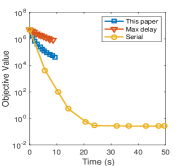
In this section, we evaluate the numerical performance of Algorithm 1 on solving two problems: the LASSO problem and the nonnegative matrix factorization (NMF). The tests were carried out on a machine with 64GB of memory and two Intel Xeon E5-2690 v2 processors (20 cores, 40 threads). All of the experiments were coded in C++ and its threading library was used for parallelization. We use the Eigen library for numerical linear algebra operations. To measure the delay, we use an atomic variable to track the number of iterations as defined in the paper. The atomic variable will be incremented by one for each update. For each thread, the delay is calculated based on the difference of the iteration counters before and after the update. For LASSO, two different settings were used. The first one sets the stepsize by the expected delay according to the analysis of this paper, and the other one used the maximum delay from liu2014asynchronous ; liu2015async-scd and is dubbed as AsySCD. We compared the async-BCU to the serial BCU, which can be regarded as a special case of Algorithm 1 with the delay $j_{k}\equiv 0,\,\forall k$. For NMF, we set the stepszie by the expected delay and test its convergence behavior with different numbers of threads.

6.1 Parameter settings

According to Theorem 4.1, the following two stepsizes were used:

$$\mbox{This paper}:\ \eta=\tfrac{1/L_{c}}{1+\kappa^{2}p^{2}/(2m)},$$ (137a)

$$\mbox{Max delay}:\ \eta=\tfrac{1/L_{c}}{1+\kappa^{2}\tau^{2}/(2m)},$$ (137b)

where $\tau$ equals the maximum number of the generated sequence of delays.

6.2 LASSO

We measure the performance of Algorithm 1 on the LASSO problem tibshirani1996-Lasso

$$\operatorname*{minimize}_{{\mathbf{x}}\in\mathbb{R}^{n}}\tfrac{1}{2}\|{\mathbf{A}}{\mathbf{x}}-{\mathbf{b}}\|_{2}^{2}+\lambda\|{\mathbf{x}}\|_{1},$$ (138)

where ${\mathbf{A}}\in\mathbb{R}^{N\times n}$, ${\mathbf{b}}\in\mathbb{R}^{N}$, and $\lambda$ is a parameter balancing the fitting term and the regularization term. We randomly generated ${\mathbf{A}}$ and ${\mathbf{b}}$ following the standard normal distribution. The size was fixed to $n=2N$ and $N=10,000$, and $\lambda=\frac{1}{N}$ was used. The Lipschitz constant $L_{c}=\max\{\|({\mathbf{A}}_{i}^{T}{\mathbf{A}}_{i})\|^{2},~{}\forall i\}$, where ${\mathbf{A}}_{i}$ represents the $i$th column block of ${\mathbf{A}}$.

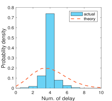
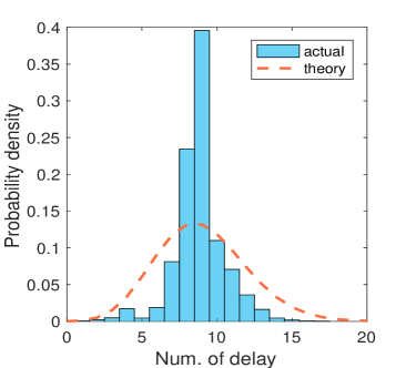
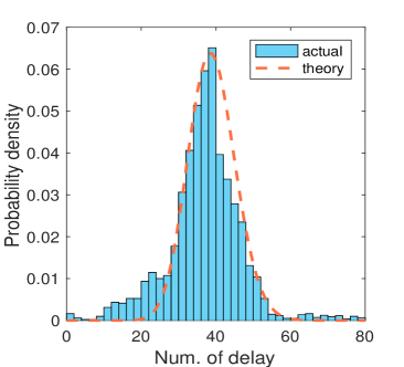
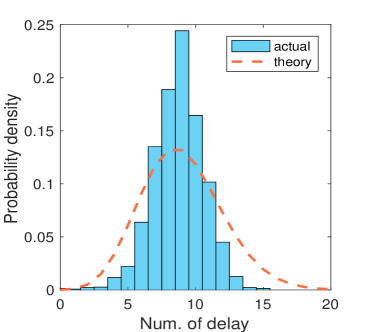
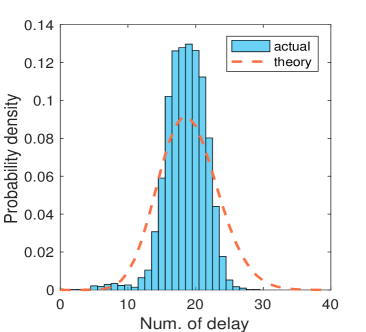
Figure 1 shows the delay distribution of Algorithm 1 with different numbers of threads. The blue bars are the normalized histogram so that the bar heights add to 1. Orange curve is the probability density function of Poisson distribution. By using 5 and 10 threads, we observe that the number of delays is concentrated on 4, and 9 respectively. When the number of threads is relatively large, the actual delay distribution closely matches with the theoretical distribution as we discussed in Section 5. For 20 threads, an interesting observation is that, the actual probability density is higher than the theoretical probability density when the number of delays is around 9. We think this is due to the architecture of the testing environment, i.e., the average delay within a CPU is smaller than the average delay across two different CPUs. We observe a similar behavior when 40 threads are used.

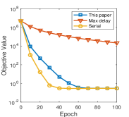
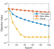
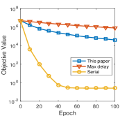
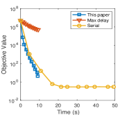
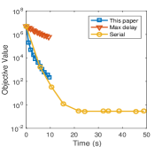
Figure 2 plots the convergence behavior of Algorithm 1 running on 40 threads with different block sizes. We partition ${\mathbf{x}}$ into $m$ equal-sized blocks with block sizes varying among $\{10,~{}50,~{}100,~{}500\}$. The results of the serial randomized coordinate descent method is also plotted for comparison. Here, one epoch is equivalent to updating all coordinates once. Comparing to the serial method, we observe that the delay does affect the convergence speed, and the affect becomes weaker as $m$ increases. Hence, Algorithm 1 can have nearly linear speed-up when the number of blocks is large. In addition, we note that the stepsize setting of AsySCD is too conservative, and Algorithm 1 with stepsize set by the expected delay converges significantly faster. However, we observed that, in general, we could not take larger stepsize than that in (137a). Some divergence behaviors are observed when using stepsizes larger than that in (137a).

5 threads	10 threads
20 threads	40 threads

Figure 1: Delay distribution behaviors of Algorithm 1 for solving LASSO (138). The tested problem has $20,000$ coordinates, and it was running with 5, 10, 20, and 40 threads.

2,000 blocks	400 blocks	200 blocks	40 blocks

Figure 2: Convergence behaviors of Algorithm 1 for solving the LASSO problem (138) with the stepsize given in (137), and also the serial randomized coordinate descent method. The tested problem has $10,000$ samples and $20,000$ coordinates that are evenly partitioned into $m$ blocks. It was simulated as running with 40 threads. We run 100 epochs for each experiments.

6.3 Nonnegative matrix factorization (NMF)

This section presents the numerical results of applying Algorithm 1 for solving the NMF problem paatero1994-NMF

$$\begin{array}[]{l}\operatorname*{minimize}\limits_{{\mathbf{X}},{\mathbf{Y}}}\ \frac{1}{2}\|{\mathbf{X}}{\mathbf{Y}}^{\top}-{\mathbf{Z}}\|_{F}^{2},\\[5.69046pt] \mbox{ s.t. }{\mathbf{X}}\in\mathbb{R}^{M\times m}_{+},{\mathbf{Y}}\in\mathbb{R}^{N\times m}_{+},\end{array}$$ (139)

where ${\mathbf{Z}}\in\mathbb{R}^{M\times N}_{+}$ is a given nonnegative matrix. We generated ${\mathbf{Z}}={\mathbf{Z}}_{L}{\mathbf{Z}}_{R}^{\top}$ with the elements of ${\mathbf{Z}}_{L}$ and ${\mathbf{Z}}_{R}$ first drawn from the standard normal distribution and then projected into the nonnegative orthant. The size was fixed to $M=N=10,000$ and $m=100$.

We treated one column of ${\mathbf{X}}$ or ${\mathbf{Y}}$ as one block coordinate, and during the iterations, every column of ${\mathbf{X}}$ was kept with unit norm. Therefore, the partial gradient Lipschitz constant equals one if one column of ${\mathbf{Y}}$ is selected to update and $\|{\mathbf{y}}_{i_{k}}^{k}\|_{2}^{2}$ if the $i_{k}$-th column of ${\mathbf{X}}$ is selected. Since $\|{\mathbf{y}}_{i_{k}}^{k}\|_{2}^{2}$ could approach to zero, we set the Lipschitz constant to $\max(0.001,\|{\mathbf{y}}_{i_{k}}^{k}\|_{2}^{2})$. This modification can guarantee the whole sequence convergence of the coordinate descent method xu2014-ecyc . Due to nonconvexity, global optimality cannot be guaranteed. Thus, we set the starting point close to ${\mathbf{Z}}_{L}$ and ${\mathbf{Z}}_{R}$. Specifically, we let ${\mathbf{X}}^{0}={\mathbf{Z}}_{L}+0.5\boldsymbol{\Xi}_{L}$ and ${\mathbf{Y}}^{0}={\mathbf{Z}}_{R}+0.5\boldsymbol{\Xi}_{R}$ with the elements of $\boldsymbol{\Xi}_{L}$ and $\boldsymbol{\Xi}_{R}$ following the standard normal distribution. All methods used the same starting point.

Figure 3 shows the delay distribution behavior of Algorithm 1 for solving NMF. The observation is similar to Figure 1. Figure 4 plots the convergence results of Algorithm 1 running with $1,~{}5,~{}10,~{}20$ and $40$ threads. From the results, we observe that Algorithm 1 scales up to 10 threads for the tested problem. Degenerated convergence is observed with 20 and 40 threads. This is mostly due to the following three reasons: (1) since the number of blocks is relatively small ($m=200$), as shown in (137a), using more threads leads to smaller stepsize, hence, slower convergence; (2) the gradient used for the current update is more staled when a relative large number of threads are used, which also leads to slow convergence; (3) high cache miss rates and false sharing also downgrade the speedup performance.

5 threads	10 threads
20 threads	40 threads

Figure 3: Delay distribution behaviors of Algorithm 1 for solving NMF (139). It was running with 5, 10, 20, and 40 threads.

Figure 4: Convergence behaviors of Algorithm 1 for solving the NMF problem (139) with the stepsize set based on the expected delay. The size of the tested problem is $M=N=10,000$ and $m=100$, i.e., 200 block coordinates, and the algorithm was tested with 1, 5, 10, 20, and 40 threads.

7 Conclusions

We have analyzed the convergence of the async-BCU method for solving both convex and nonconvex problems in a probabilistic way. We showed that the algorithm is guaranteed to converge for smooth problems if the expected delay is finite and for nonsmooth problems if the variance of the delay is also finite. In addition, we established sublinear convergence of the method for weakly convex problems and linear convergence for strongly convex ones. The stepsize we obtained depends on certain expected quantities. Assuming the given $p+1$ processors perform identically, we showed that the delay follows a Poisson distribution with parameter $p$ and thus fully determined the stepsize. We have simulated the performance of the algorithm with our determined stepsize on solving LASSO and the nonnegative matrix factorization, and the numerical results validated our analysis.

Appendix A Proofs of lemmas

The following lemma is used in other proofs several times, and it is easy to verify.

Lemma 12

For any scalar sequences $\{a_{i,j}\}$ and $\{b_{i}\}$, it holds that

$$\sum_{t=1}^{k-1}\sum_{d=k-t}^{k-1}a_{d,t} =\sum_{d=1}^{k-1}\sum_{t=k-d}^{k-1}a_{d,t},\,\forall k\geq 0,$$ (140)

$$\sum_{t=1}^{k}\sum_{d=0}^{t-1}a_{d,t} =\sum_{d=0}^{k-1}\sum_{t=d+1}^{k}a_{d,t},\,\forall k\geq 0.$$ (141)

$$\sum_{t=1}^{k}\sum_{d=1}^{t-1}a_{d,t}b_{t-d} =\sum_{t=1}^{k-1}\Big{(}\sum_{d=t+1}^{k}a_{d-t,d}\Big{)}b_{t},\,\forall k\geq 0.$$ (142)

A.1 Proof of Lemma 3

Proof

Following the proof of Theorem 1 in liu2014asynchronous , we have

$$\mathbb{E}\big{[}\|\nabla f({\mathbf{x}}^{t})\|^{2}-\|\nabla f({\mathbf{x}}^{t+1})\|^{2}\big{]}$$ (143)

$$\leq 2\mathbb{E}\big{[}\|\nabla f({\mathbf{x}}^{t})\|\cdot\|\nabla f({\mathbf{x}}^{t})-\nabla f({\mathbf{x}}^{t+1})\|\big{]}\quad(\text{from }\|{\mathbf{u}}\|^{2}-\|{\mathbf{v}}\|^{2}\leq 2\|{\mathbf{u}}\|\cdot\|{\mathbf{u}}-{\mathbf{v}}\|)$$ (144)

$$\leq 2L_{r}\mathbb{E}\big{[}\|\nabla f({\mathbf{x}}^{t})\|\cdot\|{\mathbf{x}}^{t}-{\mathbf{x}}^{t+1}\|\big{]}=2\eta L_{r}\mathbb{E}\big{[}\|\nabla f({\mathbf{x}}^{t})\|\cdot\|U_{i_{t}}\nabla f({\mathbf{x}}^{t-j_{t}})\|\big{]}$$ (145)

$$\leq \eta L_{r}\left(\frac{1}{\sqrt{m}}\mathbb{E}\|\nabla f({\mathbf{x}}^{t})\|^{2}+\sqrt{m}\mathbb{E}\|U_{i_{t}}\nabla f({\mathbf{x}}^{t-j_{t}})\|^{2}\right)$$ (146)

$$= \frac{\eta L_{r}}{\sqrt{m}}\left(\mathbb{E}\|\nabla f({\mathbf{x}}^{t})\|^{2}+\mathbb{E}\|\nabla f({\mathbf{x}}^{t-j_{t}})\|^{2}\right)$$ (147)

$$= \frac{\eta L_{r}}{\sqrt{m}}\Big{(}\mathbb{E}\|\nabla f({\mathbf{x}}^{t})\|^{2}+\sum\limits_{r=0}^{t-1}q_{r}\mathbb{E}\|\nabla f({\mathbf{x}}^{t-r})\|^{2}+c_{t}\|\nabla f({\mathbf{x}}^{0})\|^{2}\Big{)}$$ (148)

and

$$\mathbb{E}\big{[}\|\nabla f({\mathbf{x}}^{t+1})\|^{2}-\|\nabla f({\mathbf{x}}^{t})\|^{2}\big{]}$$ (149)

$$\leq \mathbb{E}\big{[}\|\nabla f({\mathbf{x}}^{t+1})+\nabla f({\mathbf{x}}^{t})\|\cdot\|\nabla f({\mathbf{x}}^{t+1})-\nabla f({\mathbf{x}}^{t})\|\big{]}$$ (150)

$$\leq L_{r}\mathbb{E}\left[\big{(}2\|\nabla f({\mathbf{x}}^{t})\|+\|\nabla f({\mathbf{x}}^{t+1})-\nabla f({\mathbf{x}}^{t})\|\big{)}\|{\mathbf{x}}^{t+1}-{\mathbf{x}}^{t}\|\right]$$ (151)

$$\leq L_{r}\mathbb{E}\left[2\|\nabla f({\mathbf{x}}^{t})\|\cdot\|{\mathbf{x}}^{t+1}-{\mathbf{x}}^{t}\|+L_{r}\|{\mathbf{x}}^{t+1}-{\mathbf{x}}^{t}\|^{2}\right]$$ (152)

$$= L_{r}\mathbb{E}\left[2\eta\|\nabla f({\mathbf{x}}^{t})\|\cdot\|U_{i_{t}}\nabla f({\mathbf{x}}^{t-j_{t}})\|+\eta^{2}L_{r}\|U_{i_{t}}\nabla f({\mathbf{x}}^{t-j_{t}})\|^{2}\right]$$ (153)

$$\leq L_{r}\mathbb{E}\left[\frac{\eta}{\sqrt{m}}\|\nabla f({\mathbf{x}}^{t})\|^{2}+\eta\sqrt{m}\|U_{i_{t}}\nabla f({\mathbf{x}}^{t-j_{t}})\|^{2}+\eta^{2}L_{r}\|U_{i_{t}}\nabla f({\mathbf{x}}^{t-j_{t}})\|^{2}\right]$$ (154)

$$= \frac{\eta L_{r}}{\sqrt{m}}\mathbb{E}\|\nabla f({\mathbf{x}}^{t})\|^{2}+\left(\frac{\eta L_{r}}{\sqrt{m}}+\frac{\eta^{2}L_{r}^{2}}{m}\right)\mathbb{E}\|\nabla f({\mathbf{x}}^{t-j_{t}})\|^{2}$$ (155)

$$= \frac{\eta L_{r}}{\sqrt{m}}\mathbb{E}\|\nabla f({\mathbf{x}}^{t})\|^{2}+\left(\frac{\eta L_{r}}{\sqrt{m}}+\frac{\eta^{2}L_{r}^{2}}{m}\right)\left(\sum\limits_{r=0}^{t-1}q_{r}\mathbb{E}\|\nabla f({\mathbf{x}}^{t-r})\|^{2}+c_{t}\|\nabla f({\mathbf{x}}^{0})\|^{2}\right).$$ (156)

We first show the first inequality in (40). Note that (39) gives us

$$\textstyle\frac{1}{1-(1+M_{\rho})\frac{\eta L_{r}}{\sqrt{m}}}\leq\rho.$$ (157)

When $t=0$, we have from (143) that $\textstyle\|\nabla f({\mathbf{x}}^{0})\|^{2}-\mathbb{E}\|\nabla f({\mathbf{x}}^{1})\|^{2}\leq\frac{2\eta L_{r}}{\sqrt{m}}\|\nabla f({\mathbf{x}}^{0})\|^{2}\leq(1+M_{\rho})\frac{\eta L_{r}}{\sqrt{m}}\|\nabla f({\mathbf{x}}^{0})\|^{2}.$ Hence, $\|\nabla f({\mathbf{x}}^{0})\|^{2}\leq\rho\mathbb{E}\|\nabla f({\mathbf{x}}^{1})\|^{2}$ from (157). Now we assume that $\mathbb{E}\|\nabla f({\mathbf{x}}^{t})\|^{2}\leq\rho\mathbb{E}\|\nabla f({\mathbf{x}}^{t+1})\|^{2}$ for all $t\leq k-1$. For $t=k$, it holds from (143) and the induction assumption that

$$\mathbb{E}\|\nabla f({\mathbf{x}}^{k})\|^{2}-\mathbb{E}\|\nabla f({\mathbf{x}}^{k+1})\|^{2}$$

$$\leq \frac{\eta L_{r}}{\sqrt{m}}\left(\mathbb{E}\|\nabla f({\mathbf{x}}^{k})\|^{2}+\sum\limits_{t=0}^{k-1}q_{t}\rho^{t}\mathbb{E}\|\nabla f({\mathbf{x}}^{k})\|^{2}+c_{k}\rho^{k}\mathbb{E}\|\nabla f({\mathbf{x}}^{k})\|^{2}\right)$$

$$= \frac{\eta L_{r}}{\sqrt{m}}\left(1+\sum\limits_{t=0}^{k-1}q_{t}\rho^{t}+c_{k}\rho^{k}\right)\mathbb{E}\|\nabla f({\mathbf{x}}^{k})\|^{2}\leq\frac{\eta L_{r}}{\sqrt{m}}(1+M_{\rho})\cdot\mathbb{E}\|\nabla f({\mathbf{x}}^{k})\|^{2}.$$

Hence, we have $\mathbb{E}\|\nabla f({\mathbf{x}}^{k})\|^{2}\leq\rho\mathbb{E}\|\nabla f({\mathbf{x}}^{k+1})\|^{2}$ from (157). Therefore, we finish the induction step, and thus the first inequality of (40) holds.

Next we show the second inequality of (40). Since (39) implies $\textstyle\eta\leq\frac{\rho-1}{\frac{L_{r}}{\sqrt{m}}\left(1+M_{\rho}+\frac{(\rho-1)M_{\rho}}{\rho(1+M_{\rho})}\right)}$,

$$1+\frac{\eta L_{r}}{\sqrt{m}}+\left(\frac{\eta L_{r}}{\sqrt{m}}+\frac{\eta^{2}L_{r}^{2}}{m}\right)M_{\rho}\overset{(\ref{sm-eta-rate})}{\leq} 1+\frac{\eta L_{r}}{\sqrt{m}}(1+M_{\rho})+M_{\rho}\frac{\eta L_{r}^{2}}{m}\frac{(\rho-1)\sqrt{m}}{\rho L_{r}(1+M_{\rho})}$$ (158)

$$= 1+\frac{\eta L_{r}}{\sqrt{m}}\left(1+M_{\rho}+\frac{(\rho-1)M_{\rho}}{\rho(1+M_{\rho})}\right)\leq\rho.$$ (159)

When $t=0$, we have from (149) that

$$\mathbb{E}\|\nabla f({\mathbf{x}}^{1})\|^{2}-\|\nabla f({\mathbf{x}}^{0})\|^{2}\leq \big{(}\frac{2\eta L_{r}}{\sqrt{m}}+\frac{\eta^{2}L_{r}^{2}}{m}\big{)}\|\nabla f({\mathbf{x}}^{0})\|^{2}$$

$$\leq \left((1+M_{\rho})\frac{\eta L_{r}}{\sqrt{m}}+\frac{\eta^{2}L_{r}^{2}}{m}\right)\|\nabla f({\mathbf{x}}^{0})\|^{2}.$$

Hence, $\mathbb{E}\|\nabla f({\mathbf{x}}^{1})\|^{2}\leq\rho\|\nabla f({\mathbf{x}}^{0})\|^{2}$ holds from (158). Assume $\mathbb{E}\|\nabla f({\mathbf{x}}^{t+1})\|^{2}\leq\rho\mathbb{E}\|\nabla f({\mathbf{x}}^{t})\|^{2}$ for all $t\leq k-1$. It follows from (149) and the induction assumption that

$$\mathbb{E}\|\nabla f({\mathbf{x}}^{k+1})\|^{2}-\mathbb{E}\|\nabla f({\mathbf{x}}^{k})\|^{2}$$

$$\leq \frac{\eta L_{r}}{\sqrt{m}}\mathbb{E}\|\nabla f({\mathbf{x}}^{k})\|^{2}+\left(\frac{\eta L_{r}}{\sqrt{m}}+\frac{\eta^{2}L_{r}^{2}}{m}\right)\left(\sum\limits_{t=0}^{k-1}q_{t}\rho^{t}\mathbb{E}\|\nabla f({\mathbf{x}}^{k})\|^{2}+c_{k}\rho^{k}\mathbb{E}\|\nabla f({\mathbf{x}}^{k})\|^{2}\right)$$

$$= \left(\frac{\eta L_{r}}{\sqrt{m}}+\left(\frac{\eta L_{r}}{\sqrt{m}}+\frac{\eta^{2}L_{r}^{2}}{m}\right)\left(\sum\limits_{t=0}^{k-1}q_{t}\rho^{t}+c_{k}\rho^{k}\right)\right)\mathbb{E}\|\nabla f({\mathbf{x}}^{k})\|^{2}$$

$$\leq \left(\frac{\eta L_{r}}{\sqrt{m}}+\left(\frac{\eta L_{r}}{\sqrt{m}}+\frac{\eta^{2}L_{r}^{2}}{m}\right)M_{\rho}\right)\mathbb{E}\|\nabla f({\mathbf{x}}^{k})\|^{2}.$$

Hence, from (158), $\mathbb{E}\|\nabla f({\mathbf{x}}^{k+1})\|^{2}\leq\rho\mathbb{E}\|\nabla f({\mathbf{x}}^{k})\|^{2}$ holds, and we complete the proof. ∎

References

- (1) Beck, A., Teboulle, M.: A fast iterative shrinkage-thresholding algorithm for linear inverse problems. SIAM Journal on Imaging Sciences 2(1), 183–202 (2009)
- (2) Bertsekas, D.P.: Distributed asynchronous computation of fixed points. Mathematical Programming 27(1), 107–120 (1983)
- (3) Cannelli, L., Facchinei, F., Kungurtsev, V., Scutari, G.: Asynchronous parallel algorithms for nonconvex big-data optimization: Model and convergence. arXiv preprint arXiv:1607.04818 (2016)
- (4) Chazan, D., Miranker, W.: Chaotic relaxation. Linear Algebra and its Applications 2(2), 199–222 (1969)
- (5) Cichocki, A., Zdunek, R., Phan, A.H., Amari, S.i.: Nonnegative matrix and tensor factorizations: applications to exploratory multi-way data analysis and blind source separation. John Wiley & Sons (2009)
- (6) Cortes, C., Vapnik, V.: Support-vector networks. Machine Learning 20(3), 273–297 (1995)
- (7) Dang, C.D., Lan, G.: Stochastic block mirror descent methods for nonsmooth and stochastic optimization. SIAM Journal on Optimization 25(2), 856–881 (2015)
- (8) Davis, D.: The asynchronous PALM algorithm for nonsmooth nonconvex problems. arXiv preprint arXiv:1604.00526 (2016)
- (9) Frommer, A., Szyld, D.B.: On asynchronous iterations. Journal of Computational and Applied Mathematics 123(1), 201–216 (2000)
- (10) Grippo, L., Sciandrone, M.: On the convergence of the block nonlinear Gauss-Seidel method under convex constraints. Operations Research Letters 26(3), 127–136 (2000)
- (11) Gut, A.: Probability: A Graduate Course: A Graduate Course. Springer Science & Business Media (2006)
- (12) Hannah, R., Yin, W.: On unbounded delays in asynchronous parallel fixed-point algorithms. arXiv preprint arXiv:1609.04746 (2016)
- (13) Hildreth, C.: A quadratic programming procedure. Naval Research Logistics Quarterly 4(1), 79–85 (1957)
- (14) Hong, M., Wang, X., Razaviyayn, M., Luo, Z.Q.: Iteration complexity analysis of block coordinate descent methods. Mathematical Programming 163(1-2), 85–114 (2017)
- (15) Lai, M.J., Yin, W.: Augmented and nuclear-norm models with a globally linearly convergent algorithm. SIAM Journal on Imaging Sciences 6(2), 1059–1091 (2013)
- (16) Liu, J., Wright, S., Re, C., Bittorf, V., Sridhar, S.: An asynchronous parallel stochastic coordinate descent algorithm. In: Proceedings of the 31st International Conference on Machine Learning (ICML-14), pp. 469–477 (2014)
- (17) Liu, J., Wright, S.J.: Asynchronous stochastic coordinate descent: Parallelism and convergence properties. SIAM Journal on Optimization 25(1), 351–376 (2015)
- (18) Lu, Z., Xiao, L.: On the complexity analysis of randomized block-coordinate descent methods. Mathematical Programming 152(1-2), 615–642 (2015)
- (19) Luo, Z.Q., Tseng, P.: On the convergence of the coordinate descent method for convex differentiable minimization. Journal of Optimization Theory and Applications 72(1), 7–35 (1992)
- (20) Mokhtai, A., Koppel, A., Ribeiro, A.: A class of parallel doubly stochastic algorithms for large-scale learning. arXiv preprint arXiv:1606.04991 (2016)
- (21) Nemirovski, A., Juditsky, A., Lan, G., Shapiro, A.: Robust stochastic approximation approach to stochastic programming. SIAM Journal on Optimization 19(4), 1574–1609 (2009)
- (22) Nesterov, Y.: Efficiency of coordinate descent methods on huge-scale optimization problems. SIAM Journal on Optimization 22(2), 341–362 (2012)
- (23) Paatero, P., Tapper, U.: Positive matrix factorization: A non-negative factor model with optimal utilization of error estimates of data values. Environmetrics 5(2), 111–126 (1994)
- (24) Peng, Z., Xu, Y., Yan, M., Yin, W.: Arock: An algorithmic framework for asynchronous parallel coordinate updates. SIAM Journal on Scientific Computing 38(5), A2851–A2879 (2016)
- (25) Recht, B., Re, C., Wright, S., Niu, F.: Hogwild: A lock-free approach to parallelizing stochastic gradient descent. In: Advances in Neural Information Processing Systems, pp. 693–701 (2011)
- (26) Richtárik, P., Takáč, M.: Iteration complexity of randomized block-coordinate descent methods for minimizing a composite function. Mathematical Programming 144(1-2), 1–38 (2014)
- (27) Rockafellar, R.T., Wets, R.J.B.: Variational Analysis, vol. 317. Springer Science & Business Media (2009)
- (28) Rosenfeld, J.L.: A case study in programming for parallel-processors. Communications of the ACM 12(12), 645–655 (1969)
- (29) Strikwerda, J.C.: A probabilistic analysis of asynchronous iteration. Linear Algebra and its Applications 349(1–3), 125 – 154 (2002)
- (30) Tibshirani, R.: Regression shrinkage and selection via the lasso. Journal of the Royal Statistical Society. Series B (Methodological) pp. 267–288 (1996)
- (31) Tseng, P.: Convergence of a block coordinate descent method for nondifferentiable minimization. Journal of Optimization Theory and Applications 109(3), 475–494 (2001)
- (32) Tseng, P., Bertsekas, D.P., Tsitsiklis, J.N.: Partially asynchronous, parallel algorithms for network flow and other problems. SIAM Journal on Control and Optimization 28(3), 678–710 (1990)
- (33) Tseng, P., Yun, S.: A coordinate gradient descent method for nonsmooth separable minimization. Mathematical Programming 117(1-2), 387–423 (2009)
- (34) WhiteHouse: Big Data: Seizing Opportunities Preserving Values (2014)
- (35) Xu, Y., Yin, W.: Block stochastic gradient iteration for convex and nonconvex optimization. SIAM Journal on Optimization 25(3), 1686–1716 (2015)
- (36) Xu, Y., Yin, W.: A globally convergent algorithm for nonconvex optimization based on block coordinate update. Journal of Scientific Computing 72(2), 700–734 (2017)
- (37) Zhou, H., Li, L., Zhu, H.: Tensor regression with applications in neuroimaging data analysis. Journal of the American Statistical Association 108(502), 540–552 (2013)
- (38) Zou, H., Hastie, T., Tibshirani, R.: Sparse principal component analysis. Journal of Computational and Graphical Statistics 15(2), 265–286 (2006)