LoPub: High-Dimensional Crowdsourced Data Publication with Local Differential Privacy

Abstract

High-dimensional crowdsourced data collected from a large number of users produces rich knowledge for our society. However, it also brings unprecedented privacy threats to participants. Local privacy, a variant of differential privacy, is proposed as a means to eliminate the privacy concern. Unfortunately, achieving local privacy on high-dimensional crowdsourced data raises great challenges on both efficiency and effectiveness. Here, based on EM and Lasso regression, we propose efficient multi-dimensional joint distribution estimation algorithms with local privacy. Then, we develop a Locally privacy-preserving high-dimensional data Publication algorithm, LoPub, by taking advantage of our distribution estimation techniques. In particular, both correlations and joint distribution among multiple attributes can be identified to reduce the dimension of crowdsourced data, thus achieving both efficiency and effectiveness in locally private high-dimensional data publication. Extensive experiments on real-world datasets demonstrated that the efficiency of our multivariate distribution estimation scheme and confirm the effectiveness of our LoPub scheme in generating approximate datasets with local privacy.

I Introduction

Nowadays, with the development of various integrated sensors and crowd sensing systems, the crowdsourced information from all aspects can be collected and analyzed among various data attributes to better produce rich knowledge about the group [47, 19], thus benefiting everyone in the crowdsourced system [24]. Particularly, with high-dimensional crowdsourced data (data with multiple attributes), a lot of potential information and rules behind the data can be mined or extracted to provide accurate dynamics and reliable prediction for both group and individuals [27]. For example, both individual electricity usage and community-wide electricity usage should be captured to achieve the real-time community-aware pricing in the smart grid, which integrates the distributed energy generation as well as consumption [29, 36]. People’s historical medical records and genetic information [4, 32] can be collected and mined to help hospital staff better diagnose and monitor patients’ health status. Various environment monitoring data collected from smart phone users can make urban planning more efficient and people’s daily life more convenient [23].

However, the privacy of participants can be easily inferred or identified due to the publication of crowdsourced data [17, 43, 33], especially high-dimensional data, even though some existing privacy-preserving schemes are used. The reasons for the privacy leak are two-fold:

• Non-local Privacy. Most existing work for privacy protection focus on centralized datasets under the assumption that the server is trustable. However, in crowdsourced scenarios, direct data aggregation from distributed users can give adversaries (such as curious server and misbehaved insiders) the opportunity to identify individual privacy, even if end-to-end encryption is used. Despite the privacy protection against difference and inference attacks from aggregate queries, individual’s data may still suffer from privacy leakage before aggregation because of no guaranteed privacy on the user side (i.e., local privacy [21, 9, 20, 6]).

• Curse of High-dimensionality. In crowdsourced systems, high-dimensional data is ubiquitous. With the increase of data dimension, some existing privacy-preserving techniques like differential privacy [10] (a de-facto standard privacy paradigm), if straightforwardly applied to multiple attributes with high correlations, will become vulnerable, thereby increasing the success ratio of many reference attacks like cross-checking. According to the combination theorem [31], differential privacy degrades exponentially when multiple correlated queries are processed. From the aspect of utility, baseline differential privacy algorithms can hardly achieve reasonable scalability and desirable data accuracy due to the dimensional correlations [48].

In addition to the privacy vulnerability, a large scale of various data records collected from distributed users can imply the inefficiency of data processing. Especially in IoT applications, the ubiquitous but resource-constrained sensors and infrastructures require extremely high efficiency and low overhead. For example, privacy-preserving real-time pricing mechanism requires not only effective privacy guarantee for individuals’ electricity usages but also fast response to the dynamic changes of the demands and supplies in the smart grid [29]. Thus, it is important to provide an efficient privacy-preserving method to publish the crowdsourced high-dimensional data.

In addressing the above issues, various existing schemes demonstrated their effectiveness in terms of different perspectives. One is to provide local privacy for distributed users [14], while some recent work [40][16] have been proposed to provide a local privacy guarantee for individuals in data aggregations. However, these schemes are either inefficient or not applicable for high-dimensional data [46] because of the high computation complexity and great utility loss. The other is to privately release high dimensional data [8][46][7]. For example, Chen et al. [7] proposed to achieve differential privacy on compacted attribute clusters after dimension reduction according to the attribute correlations. However, these schemes mainly deal with the centralized dataset without local privacy guarantee for distributed data contributors. To overcome the compatibility problem between those schemes, we propose a novel scheme to publish high-dimensional crowdsourced data while guaranteeing local privacy.

I-A Contribution

Our major contributions are summarized as follows.

• In this paper, we propose a locally privacy-preserving scheme for crowdsensing systems to collect and build high dimensional data from the distributed users. Particularly, we propose an efficient algorithm for multivariate joint distribution estimation and a combined algorithm to improve the existing estimation algorithms in order to achieve both high efficiency and accuracy.

• Based on the distribution and correlation information, the dimensionality and sparsity in the original dataset can be reduced by splitting the dataset into many compacted clusters.

• After learning the marginal distribution in these compacted clusters, the server can draw a new dataset from these compacted clusters, thus achieving an approximation of the whole original crowd data while guaranteeing local privacy for individuals.

• We implement and evaluate our schemes on different real-world datasets, experimental results show that our scheme is both efficient and effective in marginal estimation as well as high-dimensional data releasing.

I-B Organization

The paper is organized as follows: In Section III, we introduce the system model in our paper. In Section IV, we present preliminaries of our approach. Then, Section V presents our proposed schemes in detail. In Section VI, we present the experiment results to validate the efficiency and effectiveness of our schemes. Last, we concludes this paper in Section VII.

II Related Work

II-A High-dimensional data

To solve the privacy issue in data releasing, differential privacy [10] was proposed to lay a mathematical privacy foundation by adding proper randomness. Examples of the use of differential privacy include the privacy-preserving data aggregation operations, where differential privacy of individuals can be guaranteed by injecting carefully-calibrated Laplacian noise [15, 22, 46, 7, 26, 37, 45]. The techniques for non-interactive differential privacy [11, 12] suffer from ”curse of dimensionality” [46, 7]. Particularly, the combination theorems [31] have pointed out that differential privacy degrades when multiple related queries are processed [35]. To deal with the correlations in high-dimensional data, different schemes have been proposed [30, 42, 46, 7, 22, 8, 48].

For example, Liu et al. [30] proposed the notion of dependent differential privacy (DDP) and dependent perturbation mechanism (DPM) to both measure and preserve the privacy with consideration of the dependence and correlations. Another solution to mitigate correlation problem is to group the correlated records into clusters and then achieve privacy on each low-dimensional cluster. Based on the data structure of dimensions, these solutions can be categorized into two classes: homogeneous and heterogeneous.

1. Homogeneous data means the data structure of all dimensions is the same. For example, in the massive text document, each dimension represents the frequency histogram of a text on the distinct words. Since the data structure is the same, basic distance metrics can be simply used to cluster the similar dimensions. For example, Kellaris et al. [22] proposed to group the data attributes with similar sensitivities together to reduce the overall sensitivity. Based on the similar idea, Wang et al. [42] proposed to group the data streams with the similar trend to achieve efficient privacy on data streams. However, both value and trend similarities cannot truly reflect the correlations in heterogeneous data.

2. Heterogeneous data refers to the high-dimensional data with different dimensions, i.e., different attribute domains. For example, personal profiles may include various attributes like gender, age, education status. Intuitive distance metrics cannot measure the correlations among heterogeneous. Therefore, Zhang et al. [46] proposed to calculate the mutual information of attribute-parent pairs and then model the correlations via a Bayesian network. Li et al. [25] proposed to use copula functions to model joint distribution for high-dimensional data. However, Copula functions cannot handle attributes with small domains, which limits its application. Chen et al. [7] proposed to directly calculate the mutual information between pairwise dimensions and build a dependency graph and junction tree to model the correlations.

However, in existing schemes [7, 46] as depicted by Figure 1, the original dataset are plainly accessed twice to learn the correlations among attributes and generate the distributions for clusters. Although calibrated noises are added separately (the $4$th and $7$th step) on the aggregation results, individual’s privacy can only be protected against the third parties from the aggregation but still be threatened by the server, who collects and aggregates the data. In addition, the two accesses are computed separately without a consistent privacy guarantee. That is, two differential privacy budgets were allocated separately but it is not clear about how to allocate the privacy budget to achieve both sufficient privacy guarantee and utility maximization. Besides, although the entire high dimensional data can be reduced into several low-dimensional clusters. The sparsity caused by combinations in each cluster still exists and may lead to lower utility. In contrast to the totally centralized setting in [7], Su et al. [39] proposed a distributed multi-party setting to publish new dataset from multiple data curators. However, their multi-party computation can only protect the privacy between data servers. Instead, individual’s local privacy in a data server cannot be guaranteed.

Also, for high-dimensional data, to show the crowd statistics and draw the correlations between attributes (variables), both privacy-preserving histogram (univariate distribution) [3] and contingency table (multivariate joint distribution) [34] are widely investigated. However, these work can not provide local privacy guarantee, thus being unable to apply to crowdsourced systems.

II-B Local privacy

However, the schemes mentioned above mainly deal with the centralized dataset. There could be scenarios, where distributed users contribute to the aggregate statistics. Despite the privacy protection against difference and inference attacks from aggregate queries, individual’s data may also suffer from privacy leakage before aggregation. Hence, the notion of local privacy has been proposed to provide local privacy guarantee for distributed users. In addition, local privacy from the end user can ensure the consistency of the privacy guarantee when there are multiple access to users’ data. Instead, non-local privacy schemes like [46] and [7] have to split and assign proper privacy budgets to different steps while accessing to the original data.

Local privacy schemes mainly focus on achieving differentially private noise via combining the data from distributed source. Many different distributed differential privacy techniques were proposed [13]. However, the local noise may be too small to cover the original data. Recently, local privacy aims to learn particular aggregation features from distributed users with some public knowledge [17, 14, 16, 40]. Sun et al. [40] proposed a percentile aggregation scheme for monitoring distributed stream. In this scheme, the possible range information is public known. For example, Groatet al. [17] proposed the technique negative surveys, which is based on randomized response techniques [44, 18], to identify the true distributions from noisy participants’ data. Similarly, Erlingsson et al. [14] proposed RAPPOR to estimate the frequencies of different strings in a candidate set. Their subsequent research [16] proposed to learn the correlations between dimensions via EM based learning algorithm. However, when the dimension is high, sparsity of data will lead to great utility loss, and moreover, the EM algorithm will have a exponentially higher complexity.

Different from these work, we propose a novel mechanism to publish high-dimensional crowdsourced data with local privacy for individuals. We compare our work with three similar existing work in the Table I. In terms of privacy model, our method is local privacy while JTree [7] is not. Our method supports high dimensional data better than RAPPOR [14] and EM [16]. Also, our method has relatively lower communication cost, time and storage complexity.

Figure 1: Main procedures of high-dimensional data publishing without local privacy

TABLE I: Comparison of LoPub with existing methods

Comparison	LoPub (Our method)	RAPPOR [14]	EM [16]	JTree [7]
Local privacy	Y	Y	Y	N
High Dimension	Y	N	N	Y
Communication	$O(\sum\nolimits_{j}|\Omega_{j}|)$	$O(\prod\nolimits_{j}|\Omega_{j}|)$	$O(\sum\nolimits_{j}|\Omega_{j}|)$	-
Time Complexity	Low	Low	Large	-
Space Complexity	Low	Large	Large	-

III System Model

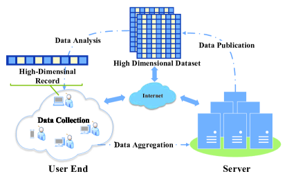
Figure 2: An architecture of distributed high dimensional private data collecting and publishing

The system model is depicted in Figure 2, where a lot of users and a central server are interconnected, constituting a crowdsourcing system. The users first collect high-dimensional data records from multiple attributes at the same time, and then send these data to the central server. The server gathers all the data and estimates high-dimensional crowdsourced data distribution with local privacy, aiming to release a privacy-preserving dataset to third-parties for conducting data analysis. In this paper, we mainly focus on data privacy, thus the detailed network model is not emphasised.

Problem Statement. Given a collection of data records with $d$ attributes from different users, our goal is to help the central server publish a synthetic dataset that has the approximate joint distribution of $d$ attributes with local privacy. Formally, let $N$ be the total number of users (i.e., data records) and sufficiently large. Let $X=\{X^{1},X^{2},\dots,X^{N}\}$ be the crowdsourced dataset, where $X^{i}$ denotes the data record from the $i$th user. We assume that there are $d$ attributes $A=\{A_{1},A_{2},\dots,A_{d}\}$ in $X$. Then each data record $X^{i}$ can be represented as $X^{i}=\{x^{i}_{1},x^{i}_{2},\dots,x^{i}_{d}\}$, where $x^{i}_{j}$ denotes the $j$th element of the $i$th user record. For each attribute $A_{j}~{}(j=1,2,\dots,d)$, we denote $\Omega_{j}=\{\omega_{j}^{1},\omega_{j}^{2},\dots,\omega_{j}^{|\Omega_{j}|}\}$ as the domain of $A_{j}$, where $\omega_{j}^{i}$ is the $i$th attribute value of $\Omega_{j}$ and $|\Omega_{j}|$ is the cardinality of $\Omega_{j}$.

With the above notations, our problem can be formulated as follows: Given a dataset $X$, we aim to release a locally privacy-preserving dataset $X^{\star}$ with the same attributes $A$ and number $N$ of users in $X$ such that

$$P_{X^{\star}}(A_{1}\dots A_{d}) \approx P_{X}(A_{1}\dots A_{d})$$ (1)

and

$$P_{X}(A_{1}\dots A_{d})\triangleq P_{X}(x^{i}_{1}=\omega_{1},\dots,x^{i}_{d}=\omega_{d})$$ (2)

$$\text{for}~{}i=1,\dots,N,\text{and}~{}~{}\omega_{1},\dots,\omega_{d}\in\Omega_{d}$$

where $P_{X}(x^{i}_{1}=\omega_{1},\dots,x^{i}_{d}=\omega_{d})$ is defined as the $d$-dimensional (multivariate) joint distribution on $X$.

To focus our research on data privacy, we assume that the central server and users are all honest-but-curious in the sense that they will honestly follow the protocols in the system without maliciously manipulating their received data. However, they may be curious about others’ data privacy and even collide to infer others’ data. In addition, the central server and users share the same public information, such as the privacy-preserving protocols (including the hash functions used) and the domain $\Omega_{j}$ for each attribute $A_{j}$ ($j=1,2,\dots,d$).

IV Preliminaries

IV-A Differential Privacy

Differential privacy is the de-facto standard for privacy guarantee on . It limits the adversaries’ ability of inferring the participation or absence of any user in a data set via adding carefully calibrated noise to the query results on the data set. The definition of $\epsilon$-differential privacy can be found in [10]. $\epsilon$ is the privacy budget (or privacy parameter) to specify the level of privacy protection and smaller $\epsilon$ means better privacy. According to the combination theorem [35], extra privacy budget will be required when multiple differential privacy mechanisms are applied on related queries. Once $\epsilon$ is run out, no more differential privacy can be guaranteed.

If a mechanism $M$ is $\epsilon$-differential privacy on dataset $D$ and a new dataset $D^{\prime}$ sampled from $D$ with uniformly sampling rate $\beta$. Then, querying $M$ on $D^{\prime}$ can guarantee a $\ln(1+\beta(e^{\epsilon}-1))-$differential privacy for dataset $D$ [28].

IV-B Local Differential Privacy

Generally, differential privacy focuses on centralized database and implicitly assumes data aggregation is trustworthy. Aiming to eliminate this assumption, local privacy was proposed for crowdsourced systems to provide a stringent privacy guarantee that data contributors trust no one [21, 9]. A formal definition of local differential privacy is given below.

Definition 1

For any user $i$, a mechanism $\mathcal{M}$ satisfies $\epsilon$-local differential privacy (or simply local privacy) if for any two data records $X^{i},Y^{i}\in\Omega_{1}\times\dots\times\Omega_{d}$, and for any possible privacy-preserving outputs $\tilde{X}^{i}\in Range(\mathcal{M})$,

$$P\left(\mathcal{M}(X^{i})=\tilde{X}^{i}\right)\leq e^{\epsilon}\cdot P\left(\mathcal{M}(Y^{i})=\tilde{X}^{i}\right),$$ (3)

where the probability is taken over $\mathcal{M}^{\prime}s$ randomness and $\epsilon$ has similar impact on privacy as in the ordinary differential privacy.

Local privacy has many applications. A typical example is the randomized response technique [44], which is widely used in the survey of people’s “yes or no” opinions about a private issue. Participants of the survey are required to give their true answers with a certain probability or random answers with the remaining probability. Due to the randomness, the surveyor cannot determine the true answers of participants individually (i.e., local privacy is guaranteed) while can predict the true proportions of alternative answers.

IV-C RAPPOR based Local Privacy

Recently, RAPPOR (Randomized Aggregatable Privacy-Preserving Ordinal Response) has been proposed for statistics aggregation [14]. RAPPOR is only applicable to one or two dimensional crowdsourced data for estimating data distribution with local privacy. The basic idea of RAPPOR is the extension of the randomized response technique. In the randomized response technique, the candidate set of the domain $\Omega$ is only a binary input $\{0,1\}$ denoting “yes or no”, whereas RAPPOR generalizes the candidate set of $\Omega$ to multiple inputs such that a sufficiently long $\{0,1\}$ bit string can be applied to the domain $\Omega$.

On users, RAPPOR consists of two phases:

1. Feature Assignment. In this phase, the dataset $X$ has only one attribute with the domain $\Omega$. For each candidate value $\omega\in\Omega$, several hash functions are used to transform $\omega$ into a $m$-bit $\{0,1\}$ string $S$ (a.k.a. a Bloom filter). Once $m$ and the number of hash functions are well chosen, this transformation can maximize the uniqueness of a bit string $S$ to represent any attribute value $\omega\in\Omega$.As suggested by [38], $m$ is proportional to the domain size $|\Omega|$, i.e., $m\propto|\Omega|$.

2. Feature Cloaking. After the Bloom filter $S$ is obtained, each bit in $S$ will be randomized to $0$ or $1$ with a certain probability, or remains unchanged with the remaining probability. This randomness is important as it endows the privacy on the original data. The more randomness, the better privacy.

On the central server, RAPPOR first gathers randomized Bloom filters from different users, and then estimates the univariate distribution as follows:

1. Aggregation. Once gathered by the central server, all the bit strings will be summed up bitwise. Then the true count of each bit can be estimated based on the randomness of the bit strings.

2. Feature Rebuilding. The hash functions used on the user side are replayed on the server side to reconstruct the Bloom filters for each $\omega\in\Omega$.

3. Distribution Estimation. Taking the Bloom filters as the feature variables, the server can estimate the univariate distribution of the single attribute via linear regression.

It is important to note that RAPPOR is only efficient in low dimensional data because when the dimension $k$ is high, the length $m_{RAPPOR}$ of Bloom filters over the multi-attribute domain $\Omega_{1}\times\Omega_{2}\times\dots\times\Omega_{k}$ will become

$$m_{RAPPOR}\propto|\Omega_{1}\times\Omega_{2}\times\dots\times\Omega_{k}|=\prod\limits_{j=1}^{k}|\Omega_{j}|,$$ (4)

which requires exponential storage space in terms of $k$.

To address this problem, Fanti et al. [16] proposed an EM (Expectation Maximization) based association learning scheme, which extends the $1$-dimensional RAPPOR to estimate the $2$-dimensional joint distribution. First, a bivariate joint distribution is initialized uniformly. Then, for each record, the conditional probability distribution of the true $2$-dimensional Bloom filters given the observed noisy record is calculated according to the Bayes’ theorem. Finally, the bivariate joint distribution is updated as the expectation of the conditional probability distributions over all records. By iterating the above steps several rounds, an estimation of the bivariate joint distribution can be obtained. However, repeating scanning all the collected RAPPOR strings in each round of EM algorithm incurs considerable computational complexity.

Some notations used in this paper are listed in Table II.

TABLE II: Notation

$N$	number of users (data records) in the system
$X$	entire crowdsourced dataset on the server side
$X^{i}$	data record from the $i$th user
$x^{i}_{j}$	$j$th element of $X^{i}$
$d$	number of attributes in $X$
$\mathbb{R}$	set of all attribute clusters
$A_{j}:$	$j$th attribute of $X$
$\Omega_{j}$	domain of $A_{j}$
$\omega_{j}$	candidate attribute value in $\Omega_{j}$
$\mathcal{H}_{j}(x)$	hash functions for $A_{j}$ that map $x$ into a Bloom filter
$s^{i}_{j}$	Bloom filter of $x^{i}_{j}$ ($S^{i}_{j}=\mathcal{H}_{j}(x^{i}_{j})$)
$s^{i}_{j}[b]$	$b$th bit of $s^{i}_{j}$
$\hat{s}^{i}_{j}$	randomized Bloom filter of $s^{i}_{j}$
$\hat{s}^{i}_{j}[b]$	$b$th bit of $\hat{s}^{i}_{j}$
$m_{j}$	length of $s^{i}_{j}$
$f$	probability of randomly flipping a bit of a Bloom filter

V LoPub: High-dimensional Data Publication with Local Privacy

We propose LoPub, a novel solution to achieve high-dimensional crowdsourced data publication with local privacy. In this section, we first introduce the basic idea behind LoPub and then elaborate the algorithmic procedures in more details.

V-A Basic idea

Privacy-preserving high-dimensional crowdsourced data publication aims at releasing an approximate dataset with similar statistical information (i.e., statistical distribution defined in Equation (1)) while guaranteeing the local privacy. This problem can be considered in four aspects:

First, to achieve local privacy, some local transformation should be designed on the user side to cloak individuals’ original data record. Then, the central server needs to obtain the statistical information, a.k.a, the distribution of original data. There are two plausible solutions. One is to obtain the $1$-dimensional distribution on each attribute independently. Unfortunately, the lack of consideration of correlations between dimensions will lose the utility of original dataset. Another is to consider all attributes as one and compute the $d$-dimensional joint distribution. However, due to combinations, the possible domain will increase exponentially with the number of dimensions, thus leading to both low scalability and the signal-noise-ratio problems [46]. Particularly, with fixed local privacy guarantee, the statistical accuracy of distribution estimation will degrade significantly with the increase of the possible domain and dimensionality. Therefore, next crucial problem is to find a solution for reducing the dimensionality while keeping the necessary correlations. Finally, with the statistical distribution information on low-dimensional data, how to synthesize a new dataset is the remaining problem.

To this end, we present LoPub, a locally privacy-preserving data publication scheme for high-dimensional crowdsourced data. Figure 3 shows the overview of LoPub, which mainly consists of four mechanisms: local privacy protection, multi-dimensional distribution estimation, dimensionality reduction, and data synthesizing.

1. Local Privacy Protection. We first propose the local transformation process that adopts randomized response technique to cloak the original multi-dimensional data records on distributed users to provide local privacy for all individuals in the crowdsourced systems. Particularly, we locally transform each attribute value to a random bit string. Then, the locally privacy-preserved data is sent to and aggregated at the central server.

2. Multi-dimensional Distribution Estimation. We then propose multi-dimensional joint distribution estimation schemes to obtain both the joint and marginal probability distribution on multi-dimensional data. Inspired by [16], we present an EM-based approach for high-dimensional estimation. Moreover, we present Lasso-based approach for fast estimation at the cost of slight accuracy degradation. Finally, we propose a hybrid approach striking the balance between the accuracy and efficiency.

3. Dimensionality Reduction. Based on the multi-dimensional distribution information, we then propose to reduce the dimensionality by identifying mutual-correlated attributes among all dimensions and split the high-dimensional attributes into several compact low-dimensional attribute clusters. In this paper, considering the heterogeneous attributes, we adopt mutual information and undirected dependency graph to measure and model the correlations of attributes, respectively. In addition, we also propose a heuristic pruning scheme to further boost the process of correlation identification.

4. Synthesizing New Dataset. Finally, we propose to sample each low-dimensional dataset according to the estimated joint or conditional distribution on each attribute cluster, thus synthesizing a new privacy-preserving dataset.

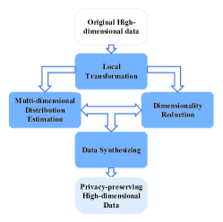
Figure 3: An overview of LoPub

V-B Local Transformation

V-B1 Design Rationale

A common framework of locally private distribution estimation is that each individual user applies a local transformation on the data for privacy protection and then sends the transformed data to the server. The server estimates the joint distribution according to the transformed data. Local transformation in our design includes two key steps: one is mapping into Bloom filters and the other is adding randomness. Particularly, Bloom filter over $\Omega$ with multiple hash functions can hash all the variables in the domain into a pre-defined space. Thus, the unique bit strings are the representative features of the original report. Then, after privacy protection by randomized responses, a large number of samples with various levels of noise are generated by individual users. After aggregation, the central server obtain a large sample space with random noises. As a result, one may estimate the distribution from the noised sample space by taking advantage of machine learning techniques such as EM algorithm and regression analysis.

Under the above framework, a key observation can be made: if features are mutual-independent, one can easily conclude that the combinations of features from different candidate sets are also mutual-independent. Therefore, when Bloom filters of each attribute are mutual-independent (i.e., no collisions for all bits), then the Cartesian product of Bloom filters of different attributes are mutual-independent. In this sense, with mutual-independent features of Bloom filters, existing machine learning techniques like EM and Lasso regression are effective for the multivariate distribution estimation. Some notations used in this paper are listed in Table II.

V-B2 Algorithmic Procedures of Local Transformation

Before describing the distribution estimation, we present that details about the local transformation. In essence, local transformation consists of three steps:

1. On each $i$th user, suppose we have an original data record $X^{i}=\{x_{1}^{i},x_{2}^{i},\dots,x_{d}^{i}\}$ with $d$ attributes. For each attribute $A_{j}\ (j=1,\dots,d)$ , we employ hash functions ${\cal H}_{j}(\cdot)$ to map $x_{j}^{i}$ to a length-$m_{j}$ bit string $s_{j}^{i}$ (called a Bloom filter). That is,

   $$s_{j}^{i}={\cal H}_{j}(x_{j}^{i})\quad(\forall j=1,\dots,d)$$

2. Each bit $s_{j}^{i}[b]~{}(b=1,2,\dots,m_{j})$ in $s_{j}^{i}$ is randomly flipped into $0$ or $1$ according to the following rule:

   $$\hat{s}_{j}^{i}[b]=\begin{cases}s_{j}^{i}[b],~{}~{}&\text{with probability of}~{}1-f\\ 1,~{}~{}&\text{with probability of}~{}f/2\\ 0,~{}~{}&\text{with probability of}~{}f/2\\ \end{cases}$$ (5)

   where $f\in(0,1)$ is a user-controlled flipping probability that quantifies the level of randomness for local privacy.

3. Having flipped each bit string $s_{j}^{i}$ bit by bit into randomized Bloom filter $\hat{s}_{j}^{i}\ (j=1,\dots,d)$, we concatenates $\hat{s}_{1}^{i},\dots,\hat{s}_{d}^{i}$ to obtain a stochastic $(d\cdot m_{j})$-bit vector:

   $$\big{[}\hat{s}_{1}^{i}[1],\dots,\hat{s}_{1}^{i}[m_{1}]~{}\vline~{}\hat{s}_{2}^{i}[1],\dots,\hat{s}_{2}^{i}[m_{2}]~{}\vline~{}\dots~{}\vline~{}\hat{s}_{d}^{i}[1],\dots,\hat{s}_{d}^{i}[m_{d}]\big{]}$$

   and send it to the server with guaranteed local privacy.

Example 1

TABLE III: An example of census data $X$ of college alumni

	Age	Gender	Education	Income Level
$u_{1}$	29	M	college	working
$u_{2}$	35	F	master	low-middle
$u_{3}$	45	F	college	working
$\dots$	…	…	…	…
$u_{N}$	49	M	phd	up-middle

TABLE IV: Attribute domain information of dataset $X$

j	$A_{j}$	$\Omega_{j}$	$|\Omega_{j}|$
1	Age	$[25,60]$	35
2	Gender	$\{\text{M},\text{F}\}$	2
3	Education	$\{\text{college},\text{master},\text{phd}\}$	3
4	Income	$\{\text{working},\text{low-middle},\text{up-middle},\text{affluent}\}$	4

TABLE V: Bloom strings of attribute domain ${\cal H}_{j}(\Omega_{j})$

j	$A_{j}$	${\cal H}_{j}(\Omega_{j})$	$|{\cal H}_{j}(\Omega_{j})|$
1	Age	$\{100100111,\dots,01010110\}$	35
2	Gender	$\{01,10\}$	2
3	Education	$\{0101,0110,1100\}$	3
4	Income	$\{0110,0011,1001,1100\}$	4

TABLE VI: Privacy-preserving bit strings of $X$

	Age	Gender	Education	Income Level
$u_{1}$	10010111	10	0111	0100
$u_{2}$	01110001	00	1110	0111
$u_{3}$	01011100	10	0100	0010
$\dots$	…	…	…	…
$u_{N}$	11010100	00	0110	1111

Tabel III shows a simplified example of original census dataset $X$ with 4 attributes {“Age”,“Gender”, “Education”, ”Income Level”}, where each record is contributed by user $u_{i}$, $1\leq i\leq N$. Consider data record $X^{2}=\{\emph{\text{35}, \text{F}, \text{Master}, \text{Low-middle}}\}$ on $2$nd user. To guarantee local privacy, we first use hash functions ${\cal H}_{j}(\cdot)$ to map $j$th element of $X^{2}$ into a bit string. Next, having been randomly flipped bit by bit, these bit strings become

$$\begin{array}[]{lllll}{\cal H}_{1}(\textrm{35})&=&\{01011001\}&\Rightarrow&\{10\underline{0}101\underline{1}1\}\\ {\cal H}_{2}(\textrm{F})&=&\{10\}&\Rightarrow&\{\underline{0}0\}\\ {\cal H}_{3}(\textrm{master})&=&\{0110\}&\Rightarrow&\{\underline{1}110\}\\ {\cal H}_{4}(\textrm{low-middle})&=&\{0011\}&\Rightarrow&\{0\underline{1}11\}\\ \end{array}$$

where underlined bits have been changed according to Equation (5). Finally, the concatenation of these randomized bit strings for each attribute yields a privacy-preserving bit string for the entire record $X^{2}$

$$[10\underline{0}101\underline{1}1\underline{1}011\ \vline\ \underline{0}0\ \vline\ \underline{1}110\ \vline\ 0\underline{1}11],$$

which will be sent to the central server under local privacy. Similarly, other users should transform their data in a same way. Table VI shows the example of transformed privacy-preserving report strings received by the server. $\blacksquare$

Parameters Setup: According to the characteristic of Bloom filter [38], given the false positive probability $p$ and the number $|\Omega_{i}|$ of elements to be inserted, the optimal length $m_{j}$ of Bloom filter can be calculated as

$$m_{j}=\frac{\ln(1/p)}{(\ln 2)^{2}}|\Omega_{j}|.$$ (6)

Furthermore, the optimal number $h_{j}$ of hash functions is

$$h_{j}=\frac{m_{j}}{|\Omega_{j}|}\ln 2=\frac{\ln(1/p)}{(\ln 2)}.$$ (7)

So, the optimal $h=\frac{\ln(1/p)}{(\ln 2)}$ for all dimensions.

Privacy Analysis: Because local transformation is performed by the individual user, no one can obtain the original record $X^{i}$, local privacy can be easily achieved and we only have to analyze the privacy guarantee on the user side. According to the conclusion in [14], differential privacy obtained for each attribute on the user side is $2h\ln\left((2-f)/f\right)$, where $h$ is the number of hash functions in the Bloom filter and $f$ is the probability that a bit vector was flipped.

Since both hash operations and randomized response on all attributes are independent, then as pointed by the composition theorem [31], the overall differential privacy achieved on the user side should be

$$\epsilon=2dh\ln\left((2-f)/f\right),$$ (8)

where $d$ is the number of dimensions.

Overall, since the same transformation is done by all users independently, this $\epsilon$-local privacy guarantee is equivalent for all distributed users. In the rest of our paper, we will focus on how to achieve a better utility-privacy tradeoff from users’ privacy-preserving high-dimensional data with this privacy guarantee $\epsilon$.

Communication Overhead:

Theorem 1

The minimal communication cost $C$ after the local transformation is

$$C=\sum_{j=1}^{d}m_{j}=\frac{\ln(1/p)}{(\ln 2)^{2}}\sum_{j=1}^{d}|\Omega_{j}|.$$ (9)

Proof If we assume that the domain of each attribute is publicly known by both users and the server, then the communication cost of non-private collection is basically $\sum_{j=1}^{d}\ln|\Omega_{j}|$, which is related to the domain size. Nevertrheless, in our method with local privacy, the communication cost is $\sum_{j=1}^{d}m_{j}$, which is related to the length of Bloom filters because only randomly flipped bit strings (not original data record) are sent. $\blacksquare$

For comparison, under the same condition, when RAPPOR [14] is directly applied to the $k$-dimensional data, all $\Omega_{1}\times\dots\times\Omega_{k}$ candidate value will be regarded as $1$-dimensional data, then the cost is

$$C_{RAPPOR}=\frac{\ln(1/p)}{(\ln 2)^{2}}\prod_{j=1}^{k}|\Omega_{j}|,$$ (10)

where $\prod_{j=1}^{k}|\Omega_{j}|$ is due to the size of the candidate set $\Omega_{1}\times\dots\times\Omega_{k}$. Difference between Equation 9 and LABEL:comcost:rappor is because our LoPub, compared with straightforward RAPPOR, considers the mutual independency between multiple attributes. It should be noted that the Bloom filter length $m_{j}$ as well as communication cost $C_{LoPub}$ (or $C_{RAPPOR}$) is independent from the privacy level achieved.

V-C Multivariate Distribution Estimation with Local Privacy

V-C1 EM-based Distribution Estimation

After receiving randomized bit strings, the central server can aggregate them and estimate their joint distribution. However, the existing EM-based estimation [16] for joint distribution estimation is restricted to $2$ dimensions, which is impractical to many real-world datasets with high dimensions. Here, we propose an alternative EM-based estimation that can applies to $k$-dimensional dataset ($2\leq k\leq d$) with provable complexity analysis.

Before illustrating our algorithm, we first introduce the following notations. Without loss of generality, we consider $k$ specified attributes as $A_{1}$, $A_{2}$, $\dots$, $A_{k}$ and their index collection $\mathcal{C}=\{1,2,...,k\}$. For simplicity, the event $A_{j}=\omega_{j}$ or $x_{j}=\omega_{j}$ is abbreviated as $\omega_{j}$. For example, the prior probability $P(x_{1}=\omega_{1},x_{2}=\omega_{2},\dots,x_{k}=\omega_{k})$ can be simplified into $P(\omega_{1}\omega_{2}\dots\omega_{k})$ or $P(\omega_{\mathcal{C}})$.

Algorithm 1 depicts our EM-based approach for estimating $k$-dimensional joint distribution. More specifically, it consists of the following five main steps.

Algorithm 1 EM-based $k$-dimensional Joint Distribution

0:  

$\mathcal{C}$	: attribute indexes cluster, i.e., $\mathcal{C}=\{1,2,...,k\}$
$A_{j}$	: $k$-dimensional attributes $(1\leq j\leq k)$,
$\Omega_{j}$	: domain of $A_{j}$ $(1\leq j\leq k)$,
$\hat{s}_{j}^{i}$	: observed Bloom filters $(1\leq i\leq N)$ $(1\leq j\leq k)$,
$f$	: flipping probability,
$\delta$	: convergence accuracy.

0:  $P(A_{\mathcal{C}})$: joint distribution of $k$ attributes specified by $\mathcal{C}$.

1:  initialize $P_{0}(\omega_{\mathcal{C}})=1/(\prod\limits_{j\in\mathcal{C}}|\Omega_{j}|)$.

2:  for each $i=1,\dots,N$ do

3:     for each $j\in\mathcal{C}$ do

4:        compute $P(\hat{s}^{i}_{j}|\omega_{j})=\prod\nolimits_{b=1}^{m_{j}}(\frac{f}{2})^{\hat{s}_{j}^{i}[b]}(1-\frac{f}{2})^{1-\hat{s}_{j}^{i}[b]}$.

5:     end for

6:     compute $P(\hat{s}^{i}_{\mathcal{C}}|\omega_{\mathcal{C}})=\prod\limits_{j\in\mathcal{C}}P(\hat{s}^{i}_{j}|\omega_{j})$.

7:  end for

8:  initialize $t=0$                         /* number of iterations */

9:  repeat

10:     for each $i=1,\dots,N$ do

11:        for each $(\omega_{\mathcal{C}})\in\Omega_{1}\times\Omega_{2}\times\dots\times\Omega_{k}$ do

12:           compute $P_{t}(\omega_{\mathcal{C}}|\hat{s}^{i}_{\mathcal{C}})=\frac{P_{t}(\omega_{\mathcal{C}})\cdot P(\hat{s}_{\mathcal{C}}^{i}|\omega_{\mathcal{C}})}{\sum\limits_{\omega_{\mathcal{C}}}P_{t}(\omega_{\mathcal{C}})P(\hat{s}^{i}_{\mathcal{C}}|\omega_{\mathcal{C}})}$

13:        end for

14:     end for

15:     set $P_{t+1}(\omega_{\mathcal{C}})=\frac{1}{N}\sum_{i=1}^{N}P_{t}(\omega_{\mathcal{C}}|\hat{s}^{i}_{\mathcal{C}})$

16:     update $t=t+1$

17:  until $\max\limits_{\omega_{\mathcal{C}}}P_{t}(\omega_{\mathcal{C}})-\max\limits_{\omega_{\mathcal{C}}}P_{t-1}(\omega_{\mathcal{C}})\leq\delta$.

18:  return  $P(A_{\mathcal{C}})=P_{t}(\omega_{\mathcal{C}})$

1. Before executing EM procedures, we set an uniform distribution $P(\omega_{1}\omega_{2}\dots\omega_{k})=1/(\prod\limits_{j=1}^{k}|\Omega_{j}|)$ as the initial prior probability.

   Example 2

   For simplicity, we consider the joint distribution on attributes $A_{2}A_{3}$ (a.k.a. “Gender” and “Education”). First, we initialize the probability on each combination as $P(A_{2}A_{3})=1/(|\Omega_{2}|\times|\Omega_{3}|)=1/6$.

2. According to Equation (5), each bit $s_{j}^{i}[b]$ will be changed with probability $\frac{f}{2}$ and remains unchanged with probability $1-\frac{f}{2}$. By comparing the bits $\mathcal{H}_{j}(\omega_{j})$ with the randomized bits, the conditional probability $P(\hat{s}^{i}_{j}|\omega_{j})$ can be computed (see line 4 of Algorithm 1).

   Example 3

   We calculate the conditional probability $P(\hat{s}^{i}_{j}|\omega_{j})$ of each attribute $A_{j}~{}(j=2,3)$. For example, on attribute $A_{3}$ (or Education), in the case of privacy parameter $f=1/2$, we have

   $$P(\hat{s}^{1}_{3}|A_{3}=\text{college})$$ (11)

   $$= P(\hat{s}^{1}_{3}=0111|{\cal H}_{3}=0101)$$

   $$= P(\hat{s}^{1}_{3}[1]=0|{\cal H}_{3}[1]=0)\times$$

   $$P(\hat{s}^{1}_{3}[2]=1|{\cal H}_{3}[2]=1)\times$$

   $$P(\hat{s}^{1}_{3}[3]=1|{\cal H}_{3}[3]=0)\times$$

   $$P(\hat{s}^{1}_{3}[4]=1|{\cal H}_{3}[4]=1)$$

   $$= (1-\frac{f}{2})(1-\frac{f}{2})(\frac{f}{2})(1-\frac{f}{2})=\frac{27}{256}$$

   Similarly, the conditional probabilities on other combinations can also be obtained.

3. Due to the independence between attributes (and their Bloom filters), the joint conditional probability can be easily calculated by combining each individual attribute, so $P(\hat{s}^{i}_{1}\hat{s}^{i}_{2}\dots\hat{s}^{i}_{k}|\omega_{1}\omega_{2}\dots\omega_{k})=\prod\nolimits_{j=1}^{k}P(\hat{s}^{i}_{j}|\omega_{j})$.

   Example 4

   The joint conditional probability $P(\hat{s}^{1}_{2}\hat{s}^{1}_{3}|A_{2}A_{3})$ of attributes $A_{2}A_{3}$ can be enumerated. For example, the probability that $u_{1}$ is “a female (Gender=F) alumni with phd degree and low-middle income” can be computed as

   $$P(\hat{s}^{1}_{2}\hat{s}^{1}_{3}|A_{2}=\text{F},A_{3}=\text{phd})$$ (12)

   $$= P(\hat{s}^{1}_{2}|A_{2}=\text{F})\times P(\hat{s}^{1}_{3}|A_{3}=\text{phd})$$

   Similarly, the conditional probability $P(\hat{s}^{1}_{2}\hat{s}^{1}_{3}|A_{2}A_{3})$ on other $5$ candidate combinations of $A_{2}A_{3}$ can be obtained.

4. Given all the conditional distributions of one particular combination of bit strings, their corresponding posterior probability can be computed by the Bayes’ Theorem,

   $$P_{t}(\omega_{1}\omega_{2}\dots\omega_{k}|\hat{s}^{i}_{1}\hat{s}^{i}_{2}\dots\hat{s}^{i}_{k})$$ (13)

   $$= \frac{P_{t}(\omega_{1}\omega_{2}\dots\omega_{k})\cdot P(\hat{s}_{1}^{i}\hat{s}_{2}^{i}\dots\hat{s}_{k}^{i}|\omega_{1}\omega_{2}\dots\omega_{k})}{\sum\limits_{\omega_{1}}\sum\limits_{\omega_{2}}\dots\sum\limits_{\omega_{k}}P_{t}(\omega_{1}\omega_{2}\dots\omega_{k})P(\hat{s}^{i}_{1}\hat{s}^{i}_{2}\dots\hat{s}^{i}_{k}|\omega_{1},\omega_{2}\dots\omega_{k})}.$$

   Where $P_{t}(\omega_{1}\omega_{2}\dots\omega_{k})$ is the $k-$dimensional joint probability at the $t$th iteration.

   Example 5

   Given the privacy-preserving bit string $\hat{s}^{1}_{2}\hat{s}^{1}_{3}$, the posterior probability $P(A_{2}A_{3}|\hat{s}^{1}_{2}\hat{s}^{1}_{3})$ at the first iteration can be computed such as

   $$P(A_{2}=\text{F},A_{3}=\text{phd}|\hat{s}^{1}_{2}\hat{s}^{1}_{3})$$ (14)

   $$= \frac{P_{1}(A_{2}=\text{F},A_{3}=\text{phd})\cdot P(\hat{s}^{1}_{2}\hat{s}^{1}_{3}|A_{2}=\text{F},A_{3}=\text{phd})}{\sum\limits_{\omega_{2}\in\Omega_{2}}\sum\limits_{\omega_{3}\in\Omega_{3}}P_{1}(\omega_{2}\omega_{3})\cdot P(\hat{s}^{1}_{2}\hat{s}^{1}_{3}|\omega_{2}\omega_{3})}$$

   Similarly, after observing the privacy-preserving bit string $10~{}0111~{}0100$ ($\hat{S}^{1}$), all posterior probabilities of different combinations of $A_{2}A_{3}$ can be obtained.

5. After identifying posterior probability for each user, we calculate the mean of the posterior probability from a large number of users to update the prior probability. The prior probability is used in another iteration to compute the posterior probability in the next iteration. The above EM-like procedures are executed iteratively until convergence, i.e., the maximum difference between two estimations is smaller than the specified threshold $\max P_{t}(\omega_{1}\omega_{2}\dots\omega_{k})-\max P_{t-1}(\omega_{1}\omega_{2}\dots\omega_{k})\geq\delta$.

   Example 6

   For each observed privacy-preserving bit string $\hat{S}^{i}~{}(i=1,2,\dots,N)$, the posterior probability $P(A_{2}=\text{F},A_{3}=\text{phd}|\hat{S}^{i})$ for each combination can be obtained by the above procedures, Then, the prior probability $P(A_{2}=\text{F},A_{3}=\text{phd})$ is updated by the mean value of $N$ (here we take the $4$ records $u_{1},u_{2},u_{3},\text{and}~{}u_{N}$ in the table) posterior probabilities as

   $$P_{1}(A_{2}=\text{F},A_{3}=\text{phd})$$ (15)

   $$= \frac{1}{N}\sum_{i=1}^{N}P(A_{2}=\text{F},A_{3}=\text{phd},|\hat{S}^{i})$$

   So, instead of initial probability $P_{0}(A_{2}=\text{F},A_{3}=\text{phd})=1/6=0.1667$, the updated prior probabilities $P_{1}(A_{2}=\text{F},A_{3}=\text{phd})$ (should be about $0.1564$ in our example) will be used in the next iteration. Similarly, the initial probabilities of other $5$ combinations will be updated for the next iteration.

The above algorithm can converge to a good estimation when the initial value is well chosen. EM-based $k$-dimensional joint distribution estimation will also fail when converging to local optimum. Especially when $k$ increases, there will be many local optimum to prevent good convergence because sample space of all combinations in $\Omega_{j_{1}}\times\Omega_{j_{2}}\times\dots\times\Omega_{j_{k}}$ explodes exponentially.

Complexity: Before the analysis of complexity, we should note that number of user records $N$ needs to be sufficiently large according to the analysis in [14], i.e., $N\gg v^{k}$, where $v$ denotes the average size of $|\Omega_{j}|$, otherwise it is difficult to estimate reliably from a small sample space with low signal-noise-ratio.

Theorem 2

Suppose that the average length of $m_{j}$ is $m$ and the average $|\Omega_{j}|$ is $v$. Then, the time complexity of Algorithm 1 is

$$O\big{(}Nkmv^{k}+tNv^{2k}\big{)}.$$ (16)

Proof EM-based estimation will scan all $N$ users’ bit strings with the length of $km$ one by one to compute the conditional probability for $v^{k}$ different combinations, the time complexity basically can be estimated as $O(N(km)(v^{k}))$. Also, in the $t$th iteration, computing the posterior probability of each combination when observing each bit string will incur the time complexity of $O(tN(v^{k})^{2})$. As a consequence, the overall time complexity is $O\big{(}tNv^{2k}+Nkmv^{k}\big{)}$. $\blacksquare$

Theorem 3

The space complexity of Algorithm 1 is

$$O\big{(}Nkm+2Nv^{k}\big{)}.$$ (17)

Proof In Algorithm 1, the necessary storage includes $N$ users’ bit strings with the length of $km$, so it is $O(Nkm)$. The prior probabilities on $k$ dimensions is $O(v^{k})$. The conditional probabilities and posterior probabilities on $v^{k}$ candidates for all bit strings is $O(2Nv^{k})$. So, the overall complexity is $O\big{(}Nkm+2Nv^{k}+v^{k}\big{)}=O\big{(}Nkm+2Nv^{k}\big{)}$ since $N$ is the dominant variable. $\blacksquare$

According to Theorem 2, the space overhead could be daunting when either $N$ or $k$ is large. This makes the performance of EM-based $k$-dimensional distribution estimation degrade dramatically and not applicable to high dimensional data.

V-D Lasso-based Multivariate Distribution Estimation

To improve the efficiency of the $k$-dimensional joint distribution estimation, we present a Lasso regression-based algorithm here. As mentioned in Section V-B1, the bit strings are the representative features of the original report. After randomized responses and flipping, a large number of samples with various levels of noise will be generated by individual users. So, one may consider that the central server receives a large number of samples from specific distribution, however, with random noise. In this sense, one may estimate the distribution from the noised sample space by taking advantage of linear regression $\vec{\mathbf{y}}=\mathbf{M}\beta$, where $\mathbf{M}$ is predictor variables and $\vec{\mathbf{y}}$ is response variable, and $\beta$ is the regression coefficient vector. The determinism of Bloom filter can guarantee that the features (predictor variables $\mathbf{M}$) re-extracted at the server side are the same as the user side. Moreover, response variable $\vec{\mathbf{y}}$ can be estimated from the randomized bit strings according to the statistic characters of known $f$. Therefore, the only problem is to find a good solution to the linear regression $\vec{\mathbf{y}}=\mathbf{M}\beta$. Obviously, $k$-dimensional data may incur a output domain $\Omega_{1}\times...\times\Omega_{k}$ with the size of $|\Omega_{1}|\times...\times|\Omega_{k}|$, which increases exponentially with $k$. With fixed $N$ entries in the dataset $X$, the frequencies of many combination $\omega_{1}\omega_{2}...\omega_{k}\in\Omega_{1}\times...\times\Omega_{k}$ are rather small or even zero. So, $\mathbf{M}$ is actually sparse and only part of the sparse but effective predictor variables need to be chosen. Otherwise, the general linear regression techniques will lead to overfitting problem. Fortunately, Lasso regression [41] is effective to solve the sparse linear regression by choosing predictor variables.

Algorithm 2 Lasso-based $k$-dimensional Joint Distribution

0:    

$\mathcal{C}$	: attribute indexes cluster i.e., $\{1,2,...,k\}$,
$A_{j}$	: $k$-dimensional attributes $(1\leq j\leq k)$,
$\Omega_{j}$	: domain of $A_{j}$ $(1\leq j\leq k)$,
$\hat{s}_{j}^{i}$	: observed Bloom filters $(1\leq i\leq N)$ $(1\leq j\leq k)$,
$f$	: flipping probability.

0:     $P(A_{\mathcal{C}})$: joint distribution of $k$ attributes specified by $\mathcal{C}$ .

1:  for each $j\in\mathcal{C}$ do

2:     for each $b=1,2,\dots,m_{j}$ do

3:        compute $\hat{y}_{j}[b]=\sum\nolimits_{i=1}^{N}\hat{s}_{j}^{i}[b]$

4:        compute $y_{j}[b]=(\hat{y}_{j}[b]-fN/2)/(1-f)$

5:     end for

6:     set $\mathcal{H}_{j}(\Omega_{j})=\{\mathcal{H}_{j}(\omega)~{}\vline~{}\forall\omega\in\Omega_{j}\}$

7:  end for

8:  set $\vec{\mathbf{y}}=\big{[}y_{1}[1],\dots,y_{1}[m_{1}]~{}\vline~{}y_{2}[1],\dots,y_{2}[m_{2}]~{}\vline~{}\dots~{}\vline~{}y_{k}[1],\dots,y_{k}[m_{k}]\big{]}$

9:  set $\mathbf{M}=\big{[}\mathcal{H}_{1}(\Omega_{1})\times\mathcal{H}_{2}(\Omega_{2})\times\dots\times\mathcal{H}_{k}(\Omega_{k})\big{]}$

10:  compute $\vec{\bm{\beta}}=\textsf{Lasso\_regression}(\mathbf{M},\vec{\mathbf{y}})$

11:  return  $P(A_{\mathcal{C}})=\vec{\bm{\beta}}/N$

Our Lasso-based estimation is described in Algorithm 2 and consists of the following four major steps.

1. After receiving all randomized Bloom filters from $N$ nodes, for each bit $b$ in each attribute $j$, the central server counts the number of $1^{\prime}s$ as $\hat{y}_{j}[b]=\sum\nolimits_{i=1}^{N}\hat{s}_{j}^{i}[b]$.

   Example 7

   In Table VI, each bit is counted to obtain the sum. With current $4$ records, the count vector is $(2,0\ \vline\ 1,4,3,1)$.

2. The true count sum of each bit $y_{j}[b]$ can be estimated as $y_{j}[b]=(\hat{y}_{j}[b]-fN/2)/(1-f)$ according to the randomized response applied to the true count. These count sums of all bits form a vector $\vec{\mathbf{y}}$ with the length of $\sum\nolimits_{j=1}^{k}m_{j}$.

   Example 8

   With the count vector $(2,0\ \vline\ 1,4,3,1)$, the true counts on each bit can be estimated as $(2-0.5*4/2)/(0.5)=2$, $(0-0.5*4/2)/0.5=-2$, $(1-0.5*4/2)/0.5=0$, $(4-0.5*4/2)/0.5=6$, and $(3-0.5*4/2)/0.5=4$. Therefore, the true count vector is $(2,-2\ \vline\ 0,6,4,0)$.

3. To construct the features of the overall candidate set of attribute $\omega_{1}\dots\omega_{k}$, the Bloom filters on each dimension $\Omega_{j}$ is re-implemented by the server with the same hash functions $\mathcal{H}_{j}()$ on the user end. Suppose all distinct Bloom filters on $\Omega_{j}$ are $\mathcal{H}_{j}(\Omega_{j})=\{\mathcal{H}_{j}(\omega)~{}\vline~{}\forall\omega\in\Omega_{j}\}$, where they are orthogonal with each other. The candidate set of Bloom filters is then $\mathbf{M}=\big{[}\mathcal{H}_{1}(\Omega_{1})\times\mathcal{H}_{2}(\Omega_{2})\times\dots\times\mathcal{H}_{k}(\Omega_{k})\big{]}$ and the members in $\mathbf{M}$ are still mutual orthogonal.

   Example 9

   By Cartesian product of multiple Bloom filters of different individual attributes, the Bloom filters of all candidate attribute combinations can be reconstructed. For example, the case that “a male alumni with master degree and high-middle income” can be represented by the concatenated Bloom filter ${\cal{H}}_{2}(\text{M}){\cal{H}}_{3}(\text{master})=010110$. Similarly, all $|\Omega_{2}|\times|\Omega_{3}|=2*3=6$ candidate combinations can reconstruct their corresponding Bloom filters as $010101$, $010110$, $011100$, $100101$, $100110$, $101100$. Therefore, the candidate matrix $\mathbf{M}$ can be represented as

   $$\mathbf{M}=\left[\begin{matrix}0&1&0&1&0&1\\ 0&1&0&1&1&0\\ 0&1&1&1&0&0\\ 1&0&0&1&0&1\\ 1&0&0&1&1&0\\ 1&0&1&1&0&0\end{matrix}\right]$$ (18)

   Similar demonstration is also shown in Figure 4.

4. Fit a Lasso regression model to the counter vector $\vec{\mathbf{y}}$ and the candidate matrix $\mathbf{M}$, and then choose the non-zero coefficients as the corresponding frequencies of each candidate string. By reshaping the coefficient vector into a $k$-dimensional matrix by natural order and dividing with $N$, we can get the $k$-dimensional joint distribution estimation $P(A_{1}A_{2}\dots A_{k})$. For example, in Figure. 4, we fit a linear regression to $\mathbf{y}_{12}$ and the candidate matrix $\mathbf{M}$ to estimate the joint distribution $P_{A_{1}A_{2}}$.

   Example 10

   Suppose $\vec{\mathbf{\beta}}=[p_{11},p_{12},p_{13},p_{21},p_{22},p_{23}]$ represents the frequency of $6$ combinations of $A_{2}$ and $A_{3}$. Then, without noises caused by random flipping, there should be the only $\vec{\mathbf{\beta}}$ satisfying the linear equations

   $$\vec{\mathbf{\beta}}\cdot\mathbf{M}=\vec{\mathbf{y}},$$ (19)

   However, since $\vec{\mathbf{y}}$ is an estimated vector with noises, $\vec{\mathbf{\beta}}$ cannot be directly solved. Therefore, linear regression techniques can be used to capture the best $\vec{\mathbf{\beta}}$, which includes the frequency entries for possible combinations of $A_{2}$ and $A_{3}$. So $\vec{\mathbf{\beta}}/N$ is the ratio of frequencies and the estimated probability of $P(A_{2}A_{3})$.

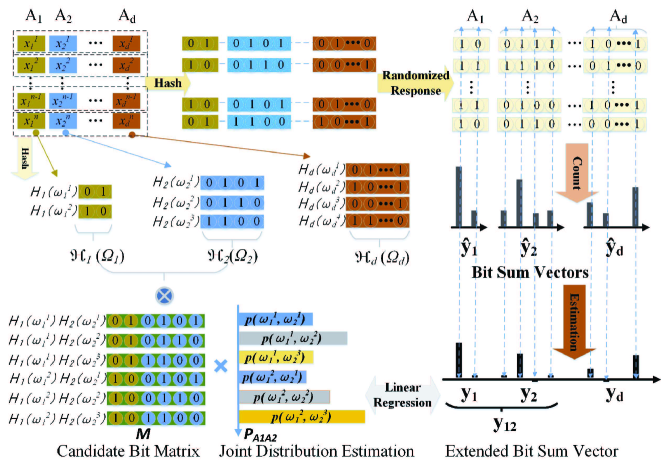
Figure 4: Illustration of Lasso-based Multivariate Joint Distribution Estimation

Generally, the regression operation, the core of the estimation, will lose accuracy only when there are many collisions between Bloom filter strings. However, as mentioned in Section V-B1, if there is no collision in the bit strings of each single dimension, then there is no collision in conjuncted bit strings of different dimensions. In fact, the probability of collision in conjuncted bit strings will not increase with dimensions. For example, suppose the collision rate of Bloom filter in one dimension is $p$, then the collision rate will decrease to $p^{k}$ when we connect bit strings of $k$ dimensions together. Therefore, we only need to choose proper $m$ and $h$ according to Equation (6) and (7) to lower the collision probability for each dimension and then we are guaranteed to have a proper estimation for multiple dimensions.

Complexity: Compared with Algorithm 1, our Lasso-based estimation can effectively reduce the time and space complexity.

Theorem 4

The time complexity of Algorithm 2 is

$$O\big{(}v^{3k}+kmv^{2k}+Nkm\big{)}.$$ (20)

Proof Algorithm 2 involves two parts: to compute the bit counter vector, $N$ bit strings with each length of $km$ will be summed up and this operation at most incurs the complexity of $O(Nkm)$; and Lasso regression with $v^{k}$ candidates (total domain size) and $km$ samples (the length of the bit counter vector is $km$) has the complexity of $O\big{(}(v^{k})^{3}+(v^{k})^{2}(km)\big{)}$. $\blacksquare$

Based on the general assumption that $N$ dominates Equation (20), then we can see the complexity in Equation (20) is much less than Equation (16) in Theorem 2.

Theorem 5

The space complexity of Algorithm 2 is

$$O\big{(}Nkm+v^{k}km\big{)}.$$ (21)

Proof In Algorithm 2, the storage overhead consists of three parts: users’ bit strings $O(Nkm)$, a count vector with size $O(km)$, and the candidate bit matrix $\mathbf{M}$ with size $O(kmv^{k})$. Therefore, the overall space complexity of our proposed Lasso based estimation algorithm is $O\big{(}Nkm+km+v^{k}km\big{)}=O\big{(}Nkm+v^{k}km\big{)}$, which is also smaller than Equation (17) as $N$ is dominant. $\blacksquare$

The empirical results are shown in Section VI. The efficiency comes from the fact that the $N$ bit strings of length $m$ will be scanned to count sum only once and then one-time Lasso regression is fitted to estimate the distribution. In addition, Lasso regression could extract the important (i.e., frequent) features with high probability, which fits well with the sparsity of high-dimensional data.

V-D1 Hybrid Algorithm

Recall that, with sufficient samples, EM-based estimation could have good convergence but also high complexity. Instead, Lasso-based estimation can be very efficient with some estimation deviation compared with EM-based algorithm. The high complexity of EM algorithm stems from two parts: Firstly, it iteratively scans user’s reports and builds a prior likely distribution table, which has the size of $N\cdot\prod|\Omega_{j}|$. And for each record of table, the computation has to compare $\sum m_{j}$ bits. However, when the dimension is high, the combination of $\Omega_{j}$ will be very sparse and has lots of zero items. Secondly, Without prior knowledge, the initial value of the random assignment (i.e., uniform distribution) will lead to too many iterations for final convergence to occur.

To achieve a balance between the EM-based estimation and Lasso-based estimation, we also propose a hybrid algorithm Lasso+EM in Algorithm 3 that first eliminates the redundant candidates and estimates the initial value with Lasso based algorithm 2 and then refines the convergence using EM-based algorithm 1. The hybrid algorithm has two advantages:

1. The sparse candidates will be selected out by the Lasso based estimation algorithm, as shown in Steps 1,2,7,8 of Algorithm 3. So the EM algorithm can just compute the conditional probability on these sparse candidates instead of all candidates, which can greatly reduce both time and space complexity.

2. Lasso-based algorithm can give a good initial estimation of the joint distribution. Compared with using initial values with random assignments, using the initial value estimated with the Lasso-based algorithm can further boost the convergence of the EM algorithm, which is sensitive to the initial value especially when the candidate space is sparse.

Theorem 6

The time complexity of Algorithm 3 is

$$O\big{(}(v^{3k}+kmv^{2k}+Nkm)+(tN(v^{\prime})^{2}+Nkm(v^{\prime}))\big{)},$$ (22)

where $v^{\prime}$ is the average size of sparse items in $\Omega_{1}\times...\times\Omega_{k}$, and $v^{\prime}<v^{k}$.

Proof See Theorem 2 and Theorem 4, the only difference is that after the Lasso based estimation, only sparse items in $\Omega_{1}\times...\times\Omega_{k}$ are selected. $\blacksquare$

Theorem 7

The space complexity of Algorithm 3 is

$$O\big{(}Nkm+v^{k}km+2Nv^{\prime}\big{)}.$$ (23)

Proof See Theorem 3 and Theorem 5. $\blacksquare$

Algorithm 3 Lasso+EM $k$-dimensional Joint Distribution (Lasso+EM_JD)

0:  

$A_{j}$	: $k$-dimensional attributes $(1\leq j\leq k)$,
$\Omega_{j}$	: domain of $A_{j}$ $(1\leq j\leq k)$,
$\hat{s}_{j}^{i}$	: observed Bloom filters $(1\leq i\leq N)$ $(1\leq j\leq k)$,
$f$	: flipping probability.

0:  $P(A_{1}A_{2}\dots A_{k})$: $k$-dimensional joint distribution.

1:  compute $P_{0}(\omega_{1}\omega_{2}\dots\omega_{k})=\textsf{Lasso\_JD}(A_{j},\Omega_{j},\{\hat{s}_{j}^{i}\}_{i=1}^{N},f)$

2:  set $\mathcal{C}^{\prime}=\{x|x\in\mathcal{C},P_{0}(x)=0\}$.

3:  for each $i=1,...,N$ do

4:     for each $j=1,...,k$ do

5:        compute $P(\hat{s}^{i}_{j}|\omega_{j})=\prod\nolimits_{b=1}^{m_{j}}(\frac{f}{2})^{\hat{s}_{j}^{i}[b]}(1-\frac{f}{2})^{1-\hat{s}_{j}^{i}[b]}$.

6:     end for

7:     if  $\omega_{1}\omega_{2}\dots\omega_{k}\in\mathcal{C}^{\prime}$  then

8:        $P(\hat{s}^{i}_{1}\hat{s}^{i}_{2}\dots\hat{s}^{i}_{k}|\omega_{1}\omega_{2}\dots\omega_{k})=0$

9:     else

10:        compute $P(\hat{s}^{i}_{1}\hat{s}^{i}_{2}\dots\hat{s}^{i}_{k}|\omega_{1}\omega_{2}\dots\omega_{k})=\prod\nolimits_{j=1}^{k}P(\hat{s}^{i}_{j}|\omega_{j})$.

11:     end if

12:  end for

13:  initialize $t=0$                         /* number of iterations */

14:  repeat

15:     … …

16:     /* (similar to Algorithm 1) */

17:     … …

18:  until $P_{t}(\omega_{1}\omega_{2}\dots\omega_{k})$ converges.

19:  return  $P(A_{1}A_{2}\dots A_{k})=P_{t}(\omega_{1}\omega_{2}\dots\omega_{k})$

V-E Dimension Reduction with Local Privacy

V-E1 Dimension Reduction via $2$-dimensional Joint Distribution Estimation

The key to reducing dimensionality in high-dimensional dataset is to find the compact clusters, within which all attributes are tightly correlated to or dependent on each other. Inspired by [46, 7] but without extra privacy budget on dimension reduction, our dimension reduction based on locally once-for-all privacy-preserved data records consists of the following three steps:

Algorithm 4 Dimension reduction with local privacy

0:    

$A_{j}$	: $k$-dimensional attributes $(1\leq j\leq k)$,
$\Omega_{j}$	: domain of $A_{j}$ $(1\leq j\leq k)$,
$\hat{s}_{j}^{i}$	: observed Bloom filters $(1\leq i\leq N)$ $(1\leq j\leq k)$,
$f$	: flipping probability,
$\phi$	: dependency degree

0:     $\mathcal{C}_{1},\mathcal{C}_{2},...,\mathcal{C}_{l}$: attribute indexes clusters

1:  initialize $\mathbf{G}_{d\times d}=\mathbf{0}$.

2:  for each $j=1,2,\dots,d$ do

3:     estimate $P(A_{j})$ by Lasso based Algorithm 2

4:  end for

5:  for each attribute $m=1,2,\dots,d$ do

6:     for each attribute $n=m+1,m+2,\dots,d$ do

7:        estimate $P(A_{m}A_{n})$ by Lasso based Algorithm 2

8:        compute $I_{m,n}=\sum_{i\in\Omega_{m}}\sum_{i\in\Omega_{n}}p_{ij}\ln{\frac{p_{ij}}{p_{i\cdot}p_{\cdot j}}}$

9:        compute $\tau_{m,n}=\min(|\Omega_{m}|-1,|\Omega_{n}|-1)*\phi^{2}/2$

10:        if $I(m,n)\geq\tau_{mn}$ then

11:           set $G_{m,n}=G_{n,m}=1,~{}~{}G\in\mathbf{G}_{d\times d}$

12:        end if

13:     end for

14:  end for

15:  build dependency graph with $\mathbf{G}_{d\times d}$

16:  triangulate the dependency graph into a junction tree

17:  split the junction tree into several cliques $\mathcal{C}_{1},\mathcal{C}_{2},...,\mathcal{C}_{l}$ with elimination algorithm.

18:  return  $\mathbb{C}=\{\mathcal{C}_{1},\mathcal{C}_{2},...,\mathcal{C}_{l}\}$

1. Pairwise Correlation Computation. We use mutual information to measure pairwise correlations between attributes. The mutual information is calculated as

   $$I_{m,n}=\sum_{i\in\Omega_{m}}\sum_{j\in\Omega_{n}}p_{ij}\ln{\frac{p_{ij}}{p_{i\cdot}p_{\cdot j}}}$$ (24)

   where, $\Omega_{m}$ and $\Omega_{n}$ are the domains of attributes $A_{m}$ and $A_{n}$, respectively. $p_{i\cdot}$ and $p_{\cdot j}$ represent the probability that $A_{m}$ is the $i$th value in $\Omega_{m}$ and the probability that $A_{n}$ is the $j$th value in $\Omega_{n}$, respectively. Then, $p_{ij}$ is their joint probability. Particulary, both $p_{i\cdot}$ and $p_{\cdot j}$ can be learned from the direct RAPPOR scheme with Lasso regression [14]. Their joint distribution $p_{ij}$ then can be efficiently obtained with our proposed multi-dimensional marginal estimation algorithm in Section V-D.

   Example 11

   A $4\times 4$ correlation matrix $\mathbf{I}$ can be built for the example dataset of Table III to record the mutual information measure.

   $$\begin{matrix}\mathbf{I}=\left[\begin{matrix}1.00&0.05&0.03&0.16\\ 0.05&1.00&0.02&0.04\\ 0.03&0.02&1.00&0.15\\ 0.16&0.04&0.15&1.00\end{matrix}\right]\end{matrix}$$ (25)

   where $\mathbf{I}_{m,n}$ is the mutual information between $A_{m}$ and $A_{n}$, e.g., $\mathbf{I}_{2,3}=0.02$ means the mutual information between $A_{2}$ and $A_{3}$ is $0.02$.

   It should be noted that the correlations need to be learnt between all attributes pairs in heterogeneous multi-attribute data. That is to say the basic complexity is $O(d^{2})$, where $d$ is the number. And in each learning process, the complexity is decided by the distribution estimation algorithm. So, the overall complexity is quite high if the distribution estimation has large complexity. Therefore, the joint distribution estimation algorithm must be light and efficient. In addition, to further overcome the high complexity of pairwise correlation learning when $d$ is large, we also proposed a heuristic pruning scheme, which can be referred to Section V-E2

2. Dependency Graph Construction. Based on mutual information, the dependency graph between attributes can be constructed as follows. First, an adjacent matrix $\mathbf{G}_{d\times d}$ is initialized with all $0$. Then, all the attribute pairs $(A_{m},A_{n})$ are chosen to compare their mutual information with an threshold $\tau_{m,n}$, which is defined as

   $$\tau_{m,n}=\min(|\Omega_{m}|-1,|\Omega_{n}|-1)*\phi^{2}/2$$ (26)

   and $\phi~{}(0\leq\phi\leq 1)$ is a flexible parameter determining the desired correlation level. $G_{m,n}$ and $G_{n,m}$ are both set to be $1$ if and only if $I_{m,n}>\tau_{m,n}$.

   Example 12

   By comparing the correlation matrix $I$ with the dependency threshold $\tau_{m,n}$, a dependency graph represented by the adjacent matrix $\mathbf{G}$ can be built.

   $$\begin{matrix}\mathbf{G}_{4\times 4}=\left[\begin{matrix}1&0&0&1\\ 0&1&0&0\\ 0&0&1&1\\ 1&0&1&1\end{matrix}\right]\end{matrix}$$ (27)

3. Compact Clusters Building. By triangulation, the dependency graph $\mathbf{G}_{d\times d}$ can be transformed to a junction tree, in which each node represents an attribute $A_{j}$. Then, based on the junction tree algorithm, several clusters $\mathcal{C}_{1},\mathcal{C}_{2},\dots,\mathcal{C}_{l}$ can be obtained as the compact clusters of attributes, in which attributes are mutually correlated. Hence, the whole attributes set can be divided into several compact attribute clusters and the number of dimensions can be effectively reduced.

   Example 13

   By triangulation, the dependency graph can be transformed to a junction tree, in which nodes are split into different clusters. Figure 5 demonstrates an example of the junction tree built from the dependency graph. The attribute set $\{A_{1},A_{2},A_{3},A_{4},A_{5},A_{6}\}$ is split into $4$ clusters $A_{1}A_{2}$, $A_{2}A_{3}A_{5}$, $A_{2}A_{4}A_{5}$ and $A_{6}$, where $A_{2}$ and $A_{2}A_{5}$ is the separators and clusters $A_{1}A_{2}$, $A_{2}A_{3}A_{5}$, and $A_{2}A_{4}A_{5}$ are also called cliques.

   

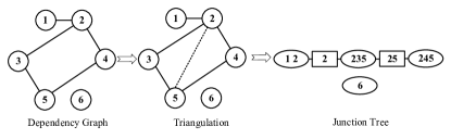
   Figure 5: Build junction tree from dependency graph

Complexity:

Theorem 8

The time complexity of Algorithm 4 is

$$O(d^{2}(v^{6}+2mv^{4}+2Nm+tN(v^{\prime})^{2}+2Nm(v^{\prime}))).$$ (28)

Proof The core of the dimension reduction process is the $d\choose 2$ times of $2$-dimensional joint distribution estimation. The complexity of each $2$-dimensional joint distribution estimation can be derived from Equation (22) when adopting the hybrid algorithm (Algorithm 3). The complexity of building junction tree on $d\times d$ dependency graph is negligible when compared with the joint distribution estimation. $\blacksquare$

Theorem 9

The space complexity of Algorithm 4 is

$$O(2Nm+2v^{2}m+2Nv^{\prime}).$$ (29)

Proof When we compute the mutual correlations between any pairs, a $2$-dimensional joint distribution estimation algorithm will be triggered with the space complexity of $O(2Nm+2mv^{2}+2Nv^{\prime})$, since $k=2$ is substituted into Equation (23). This maximum complexity dominates Algorithm 4. The space complexity of building junction tree on $d\times d$ dependency graph is negligible when compared with the joint distribution estimation. $\blacksquare$

V-E2 Entropy based Pruning Scheme

In existing work [22, 42] on homogeneous data, the correlations can be simply captured by distance metrics. However, in our work, mutual information is used to measure general correlations since heterogenous attributes (a.k.a., attributes with different domains) are also considered.

As shown in Equation (24), to calculate the mutual information of variables $X$ and $Y$, the joint probability on the joint combination is inevitable, thus making the pairwise computation of dependency necessary. Although mutual information is already simple than Kendall rank coefficients in the similar work [25], here, we still propose a pruning-based heuristic to boost this pairwise correlation learning process.

Intuitively, there are different situations in Algorithm 4: 1. When $\phi=0$ or $\phi=1$, all attributes will be considered mutually correlated or independent. Thus, there is no need to compute pairwise correlation. 2. With the increase of $\phi$ ($0<\phi<1$), less dependencies will be included in the adjacent matrix $\mathbf{G}_{d\times d}$ of dependency graph, which will become sparser. This also means that we may selectively neglect some pairs. Inspired by the relationship between mutual information and information entropy, we first heuristically filter out some portion of attributes $A_{x}$ with least relative information entropy $RH(A_{x})=H(A_{x})/|\Omega_{x}|$, and then verify the mutual information among the remaining attributes, thus reducing the pairwise computations.

Furthermore, the adjacent matrix $\mathbf{G}_{d\times d}$ of dependency graph varies in different datasets. For example, the adjacent matrix $\mathbf{G}_{d\times d}$ is rarely sparse in binary datasets but very sparse in non-binary datasets. Based on this observation, we can further simplify the calculation by finding the independency in binary datasets or finding the dependency in non-binary datasets. For example, we first set all entries of $\mathbf{G}_{d\times d}$ for a binary datasets as $1$’s and start from the attributes with least relative information entropy $RH(A_{x})=H(A_{x})/|\Omega_{x}|$ to find the uncorrelated attributes. While for non-binary datasets, we first set $\mathbf{G}_{d\times d}$ as $0$’s and then start from the attributes with largest average entropy to find the correlated attributes.

Algorithm 5 Entropy based Pruning Scheme

0:    

$A_{j}$	: $k$-dimensional attributes $(1\leq j\leq k)$,
$\Omega_{j}$	: domain of $A_{j}$ $(1\leq j\leq k)$,
$\hat{s}_{j}^{i}$	: observed Bloom filters $(1\leq i\leq N)$ $(1\leq j\leq k)$,
$f$	: flipping probability,
$\phi$	: dependency degree

0:     $\mathbf{G}_{d\times d}$: adjacent matrix $\mathbf{G}_{d\times d}$ of dependency graph of attributes $A_{j}~{}(j=1,2,...,d)$

1:  initialize $\mathbf{G}_{d\times d}=0$

2:  for each $j=1,2,\dots,k$ do

3:     compute $P(A_{j})=\textsf{JD}(A_{j},\Omega_{j},\{\hat{s}_{j}^{i}\}_{i=1}^{N},f)$

4:     compute $RH(A_{j})=-\frac{1}{|\Omega_{j}|}\sum\limits_{p\in P(A_{j})}p\log p$

5:  end for

6:  sort $list_{A}=\{A_{1},A_{2},...,A_{j}\}$ according to entropy $H(A_{j})$

7:  pick up the previous $\lfloor length(list_{A})*(1-\phi)\rfloor$ items from $list_{A}$ as a new list $list_{A^{\prime}}$

8:  …

9:  compute pairwise mutual information among $list_{A^{\prime}}$ and set dependency graph $\mathbf{G}_{d\times d}$ as in Algorithm 4.

10:  return  $\mathbf{G}_{d\times d}$

V-F Synthesizing New Dataset

For brevity, we first define $A_{C}=\{A_{j}|j\in C\}$ and $\hat{X}_{C}=\{x_{j}|j\in C\}$. Then the process of synthesizing the new dataset via sampling is shown in the following Algorithm 6.

Algorithm 6 New Dataset Synthesizing

0:    

$\mathbb{C}$	: a collection of attribute index clusters $\mathcal{C}_{1},...\mathcal{C}_{l}$,
$A_{j}$	: $k$-dimensional attributes $(1\leq j\leq k)$,
$\Omega_{j}$	: domain of $A_{j}$ $(1\leq j\leq k)$,
$\hat{s}_{j}^{i}$	: observed Bloom filters $(1\leq i\leq N)$ $(1\leq j\leq k)$,
$f$	: flipping probability,

0:     $\hat{X}$: Synthetic Dataset of $X$

1:  initialize $R=\varnothing$

2:  repeat

3:     randomly choose an attribute index cluster $C\in\mathbb{C}$

4:     estimate joint distribution $P(A_{C})$ by JD

5:     sample $\hat{X}_{C}$ according to $P(A_{C})$

6:     $\mathbb{C}=\mathbb{C}-C$, $R=R\cup C$, $\mathbb{D}=\{D\in\mathbb{C}|D\cap R\neq\varnothing\}$

7:     for each $D\in\mathbb{D}$ do

8:        estimate joint distribution $P(A_{D})$ by JD

9:        obtain conditional distribution $P(A_{D-R}|A_{D\cap R})$ from $P(A_{D})$

10:        sample $\hat{X}_{D-R}$ according to $P(A_{D-R}|A_{D\cap R})$ and $\hat{X}_{D\cap R}$

11:        $\mathbb{C}=\mathbb{C}-D$, $R=R\cup D$, $\mathbb{D}=\{D\in\mathbb{C}|D\cap R\neq\varnothing\}$

12:     end for

13:  until $\mathbb{C}=\varnothing$

14:  return  $\hat{X}$

We first initialize a set $R$ to keep the sampled attribute indexes. Then, we randomly choose an attribute index cluster $C$ to estimate the joint distribution and sample new data $\hat{X}$ in the attributes $A_{j},\forall j\in C$. Next, we remove $C$ from the cluster collection $\mathbb{C}$ into $R$, and find the connected component $\mathbb{D}$ of $C$. In the connected component, each cluster $D$ is traversed and sampled as follows. first estimate the joint distribution on the attributes $A_{D}$ by our proposed distribution estimations and obtain the conditional distribution $P(A_{D-R}|A_{D\cap R})$. Then, sample $\hat{X}_{D-R}$ according to this conditional distribution and the sampled data $\hat{X}_{D\cap R}$. After the traverse of $\mathbb{D}$, the attributes in the first connected components are sampled. Then randomly choose cluster in the remaining $\mathbb{C}$ to sample the attributes in the second connected components, until all clusters are sampled. Finally, a new synthetic dataset $\hat{X}$ is generated according to the estimated correlations and distributions in origin dataset $X$.

Theorem 10

The time complexity of Algorithm 6 is

$$O(l(v^{3k}+kmv^{2k}+Nkm+tN(v^{\prime})^{2}+Nkm(v^{\prime}))),$$ (30)

where $l$ is the number of clusters after dimension reduction and $k$ here refers to average number of dimensions in these clusters.

Proof The core of the dataset synthesizing is actually multiple ($l$ times) $k$-dimensional joint distribution estimation. $\blacksquare$

Theorem 11

The space complexity of Algorithm 6 is

$$O(Nkm+v^{k}km+2Nv^{\prime}+Nd).$$ (31)

Proof Every time, a $k$-dimensional joint distribution estimation algorithm (with space complexity of $O(Nkm+v^{k}km+2Nv^{\prime})$) is processed to draw a new dataset. A new dataset with the size $O(Nd)$ is maintained while synthesizing. $\blacksquare$

The overall process of LoPub can also be summarized as in Figure 6. Clearly, all the processed are conducted on the locally privacy-preserved data. Therefore, local privacy is guaranteed on all the crowdsourced users.

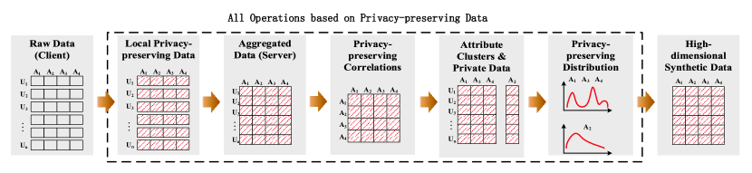
Figure 6: Main procedures of high-dimensional data publishing with local privacy

VI Evaluation

In this section, we conducted extensive experiments on real datasets to demonstrate the efficiency of our algorithms in terms of computation time and accuracy.

We used three real-world datasets: Retail [1], Adult [5], and TPC-E [2]. Retail is part of a retail market basket dataset. Each record contains distinct items purchased in a shopping visit. Adult is extracted from the 1994 US Census. This dataset contains personal information, such as gender, salary, and education level. TPC-E contains trade records of “Trade type”, “Security”, “Security status” tables in the TPC-E benchmark. It should be noted that some continuous domain were binned in the pre-process for simplicity.

Datasets	Type	#. Records ($N$)	#. Attributes ($d$)	Domain Size
Retail	Binary	27,522	16	$2^{16}$
Adult	Integer	45,222	15	$2^{52}$
TPC-E	Mixed	40,000	24	$2^{77}$

All the experiments were run on a machine with Intel Core i5-5200U CPU 2.20GHz and 8GB RAM, using Windows 7. We simulated the crowdsourced environment as follows. First, users read each data record individually and locally transform it into privacy-preserving bit strings. Then, the crowdsourced bit strings are gathered by the central server for synthesizing and publishing the high-dimensional dataset.

LoPub can be realized by combining distribution estimations and data synthesizing techniques. Thus, we implemented different LoPub realizations using Python 2.7 with the following three strategies.

1. EM_JD, the generalized EM-based multivariate joint distribution estimation algorithm.

2. Lasso_JD, our proposed Lasso-based multivariate joint distribution estimation algorithm.

3. Lasso+EM_JD, our proposed hybrid estimation algorithm that uses the Lasso_JD to filter out some candidates to reduce the complexity and replace the initial value to boost the convergence of EM_JD.

It is worth mentioning that we compared only the above algorithms since our algorithm adopts a novel local privacy paradigm on high-dimensional data. Other competitors are either for non-local privacy or on low-dimension data.

For fair comparison, we randomly chose 100 combinations of $k$ attributes from $d$ dimensional data. For simplicity, we sampled $50\%$ data from dataset Retail and $10\%$ data from datasets Adult and TPC-E, respectively. The efficiency of our algorithms is measured by computation time and accuracy. The computation time includes CPU time and IO cost. Each set of experiments is run 100 times, and the average running time is reported. To measure accuracy, we used the distance metrics AVD (average variant distance) on the three datasets, as suggested in [7], to quantify the closeness between the estimated joint distribution $P(\omega)$ and the origin joint distribution $Q(\omega)$. The AVD error is defined as

$$Dist_{\text{AVD}}(P,Q)=\frac{1}{2}\sum\limits_{\omega\in\Omega}|P(\omega)-Q(\omega)|.$$ (32)

The default parameters are described as follows. In the binary dataset Retail, the maximum number of bits and the number of hash functions used in the bloom filter are $m=32$ and $h=4$, respectively. In the non-binary datasets Adult and TPC-E, the maximum number of bits and the number of hash functions used in bloom filter are $m=128$ and $h=4$, respectively. The convergence gap is set as $0.001$ for fast convergence.

VI-A Multivariate Distribution Estimation

Here, we show the performance of our proposed distribution estimations in terms of both efficiency and effectiveness. The efficiency is measured by computation time, and the effectiveness is measured by estimation accuracy.

VI-A1 Computation Time

We first evaluate the computation time of EM_JD, Lasso_JD, and Lasso+EM_JD for the $k$-dimensional joint distribution estimation on three real datasets.

Figures 10 and 10 compare the computation time on the binary dataset Retail with both $k=3$ and $k=5$. It can be noticed that, for each dimension $k$, Lasso_JD is consistently much faster than EM_JD and Lasso+EM_JD, especially when $k$ is large. This is because EM_JD has to repeatedly scan each user’s bit string. Particularly, the time consumption of EM_JD increases with $f$ because there will be more iterations for the fixed convergence gap. In contrast, Lasso_JD uses the regression to estimate the joint distribution more efficiently. Furthermore, the complexity of Lasso+EM_JD is much less than EM_JD as the initial estimation of Lasso_JD can greatly reduce the candidate attribute space and the number of iterations needed. When $k$ is growing, the computation time of Lasso_JD increases slowly, unlike EM_JD that has a dramatic increase. This is because the time complexity of Lasso_JD is mainly subject to the number of users.

Figures 10, 10, 14, and 14 depict the computation time on non-binary datasets (Adult and TPC-E) when $k=2$ and $k=3$. As we can see, EM_JD runs with acceptable complexity on low dimension $k=2$. When $k=3$, the time complexity of EM_JD increases sharply by several times. When $k$ further increases, it does not return any result within an unacceptable time during our experiment. However, Lasso_JD takes less than a few seconds. This discrepancy is consistent with our complexity analysis, where we envision that the exponential growth of the candidate set will have a significant impact on EM_JD. So, with the initial estimation of Lasso_JD, the combined estimation Lasso+EM_JD can run relatively faster than EM_JD with limited candidate set. The computation time of EM_JD and Lasso_JD on TPC-E dataset with different $k=2$ and $k=3$ exhibits a similar tendency, as shown in Figures 14 and 14. We omitted the detailed report here due to the space constraint. It should be noted that the general time complexity on TPC-E is larger than Adult since the average candidate domain of TPC-E is larger.

VI-A2 Accuracy

Next, we compare the estimation accuracy of EM_JD,Lasso_JD, and Lasso+EM_JD on real datasets.

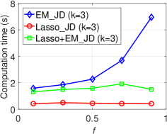
Figure 7: Estimation Time (Retail, $k=3$)

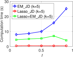
Figure 8: Estimation Time (Retail, $k=5$)

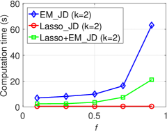
Figure 9: Estimation Time (Adult, $k=2$)

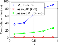
Figure 10: Estimation Time (Adult, $k=3$)

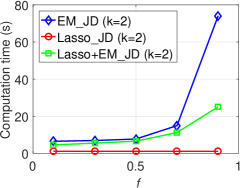
Figure 11: Estimation Time (TPC-E, $k=2$)

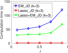
Figure 12: Estimation Time (TPC-E, $k=3$)

Figure 13: Estimation Accuracy (Retail, $k=3$)

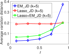
Figure 14: Estimation Accuracy (Retail, $k=5$)

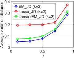
Figure 15: Estimation Accuracy (Adult, $k=2$)

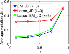
Figure 16: Estimation Accuracy (Adult, $k=3$)

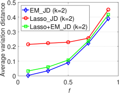
Figure 17: Estimation Accuracy (TPC-E, $k=2$)

Figure 18: Estimation Accuracy (TPC-E, $k=3$)

Figures 14 and 14 report the AVD error of EM_JD,Lasso_JD, and Lasso+EM_JD on binary dataset Retail with different dimensions $k=3$ and $k=5$. The AVD error of EM_JD is very small when $f$ is small, but when $f$ grows, it will sharply increase to as high as $0.28$. In contrast, Lasso_JD retains the error around $0.1$ even when $f=0.9$. However, in practice, when $f$ is small, i.e., $f=0.5$, the differential privacy an individual can achieve is $\epsilon=8.79$ for each dimension, which is insufficient in general. So, when $f$ is large, the AVD error of Lasso_JD is comparable to or even better than that of EM_JD. This is because Lasso regression is insensitive to $f$ when estimating the coefficients from the aggregated bit sum vectors. Nonetheless, EM_JD is sensitive to $f$ and prone to some local optimal value because it scans each record of bit strings. In comparison, Lasso+EM_JD achieves a better tradeoff between Lasso_JD and EM_JD. For example, it has less AVD error than Lasso_JD when $f$ is small and outperforms EM_JD when $f$ is large. We can also see that, the AVD error of all estimation algorithms increases with $k$, since the average frequency on $k-$dimensional combined attributes is $N/v^{k}$ and its statistical significance decreases with $k$ exponentially.

Figures 18, 18, 18 and 18 also compare the AVD error of EM_JD,Lasso_JD, and Lasso+EM_JD on the non-binary datasets Adult and TPC-E with $k=2$ and $k=3$. As can be seen, when $k=2$, the AVD error of Lasso_JD does not change with $f$ as the aggregated bit sum vector is insensitive to small $f$. While EM_JD increases with $f$ gradually due to the scan of each individual bit string. Similar to the conclusion in the binary dataset, when $f$ is large, the trend of Lasso_JD is very close to EM_JD. Besides, Lasso+EM_JD shows very similar performance to EM_JD and incurs relatively small bias. Therefore, Lasso+EM_JD achieves a good balance between utility and efficiency as it runs much faster than the baseline EM_JD. In addition, when $k$ increases $(k=3)$, the estimation error increases as well. However, Lasso+EM_D can further balance between Lasso_JD and EM_JD because the candidate set is much more sparse when $k$ is larger and Lasso+EM_JD can effectively reduce the redundant of candidate set and iterations. Similar conclusion can be made from the dataset TPC-E. Nonetheless, because of larger candidate domain, the AVD error on TPC-E is generally larger than that on Adult.

VI-B Correlation Identification

In this section, we present correlations between the multiple attributes that we can learn from locally privacy-preserved user data. Particularly, we evaluated loss ratio of dependency relationship of attributes in three datasets. The parameters used in the simulation are set as follows. The dependency threshold $0.25$ for Retail, and $0.4$ for Adult and TPC-E. The number of bits and the number of hash functions in the bloom filter are $32$ and $4$ for Retail, and $128$ and $4$ for Adult and TPC-E. The sample rate is $1$ for Retail and $0.1$ for Adult and TPC-E.

VI-B1 Accuracy

Figures 22, 22, and 22 show both the ratio of correct identification (accuracy), added (false positive) and lost (true negative) correlated pairs after estimation, respectively. From these figures, we can see all these estimation algorithms can have a relatively accurate identification among the attributes, especially EM_JD and Lasso+EM_JD algorithms. Nevertheless, generally, the accurate rate decreases with $f$ (i.e., privacy level). In Figure 22, the general accuracy identified rate is about $85\%$ when the privacy is small ($f$ is less than $0.9$). While in Figures 22 and 22, the accuracy rate is as high as $95\%$ because the dependency threshold is relatively loose as $0.4$. High accurate identification guarantees the basic correlations among attributes.

However, the incorrect identification is considered separately with false positive rate and true negative, which reflect the efficiency and effectiveness of dimension reduction. Since false positive identification just adds the correlations that were not exists, this kind of misidentification only incurs no errors but redundant correlations and extra distribution learning. Instead, true negative identification implies the loss of some correlations among attributes, thus causing information loss in our dimension reduction. For false positive identification, we can see that EM_JD algorithm and Lasso+EM_JD are less than Lasso. That is because Lasso estimation will choose the sparse probabilities and the mutual information estimated is generally high due to the concentrated probability distribution. Especially in non-binary datasets Adult and TPC-E, the sparsity is much higher, so the estimated probability distribution is more concentrated and the false positive identification rate is high.

The true negative identification in both Adult and TPC-E is small because the true correlations are not very high itself because all attributes have a large domain. Instead, the true correlations in Retail are high and almost any two attributes are dependent. Therefore, the true negative identification is comparatively higher.

VI-B2 Effectiveness of Pruning Scheme

We also validated the pruning scheme proposed in Section V-E2 with simulations on the three datasets. We first defined the dependency loss ratio as the ratio between the dependency loss after pruning with the original number of dependencies in the adjacent matrix $\mathbf{G}_{d\times d}$ of dependency graph. The complexity reduction ratio is defined as the ratio of reduced pairwise comparisons.

TABLE VII: Dependency Loss Ratio and Complexity Reduction Ratio (Adult)

$\phi$	$0.1$	$0.2$	$0.3$	$0.4$	$0.5$
$\#$. Dep (Pruning)	$88$	$38$	$22$	$12$	$6$
$\#$. Dep	$102$	$42$	$24$	$14$	$8$
Loss Ratio	$0.137$	$0.095$	$0.083$	$0.143$	$0.250$
$\#$. Pairs (Pruning)	$91$	$66$	$55$	$36$	$28$
$\#$. Pairs	$105$	$105$	$105$	$105$	$105$
Reduction Ratio	$0.133$	$0.371$	$0.476$	$0.657$	$0.733$

TABLE VIII: Dependency Loss Ratio and Complexity Reduction Ratio (TPC-E)

$\phi$	$0.1$	$0.2$	$0.3$	$0.4$	$0.5$
$\#$. Dep (Pruning)	$44$	$16$	$16$	$8$	$8$
$\#$. Dep	$46$	$24$	$20$	$10$	$10$
Loss Ratio	$0.043$	$0.333$	$0.200$	$0.200$	$0.200$
$\#$. Pairs (Pruning)	$231$	$171$	$136$	$66$	$45$
$\#$. Pairs	$276$	$276$	$276$	$276$	$276$
Reduction Ratio	$0.163$	$0.380$	$0.507$	$0.761$	$0.837$

TABLE IX: Dependency Loss Ratio and Complexity Reduction Ratio (Retail)

$\phi$	$0.1$	$0.15$	$0.2$	$0.25$	$0.3$
$\#$. Dep (Pruning)	$256$	$256$	$256$	$250$	$244$
$\#$. Dep	$240$	$240$	$238$	$220$	$200$
Loss Ratio	$-0.067$	$-0.067$	$-0.076$	$-0.136$	$-0.220$
$\#$. Pairs (Pruning)	$91$	$91$	$78$	$66$	$55$
$\#$. Pairs	$120$	$120$	$120$	$120$	$120$
Reduction Ratio	$0.242$	$0.242$	$0.350$	$0.450$	$0.512$

Tables VII, VIII, and IX illustrate the effectiveness of our proposed heuristic pruning scheme. Particularly, as shown in Tables VII and VIII, with the increase of $\phi$, which shows the strength of correlations, the number of original dependencies in dataset Adult decreases dramatically. Also, the dependencies after the heuristic pruning decrease accordingly and their number is quite close to the original. However, when $\phi$ increases, the number of pairwise comparison becomes less compared to the full pairwise comparison. So, it shows that the heuristic pruning scheme can effectively reduce the complexity with fairly small sacrifice of dependency accuracy. Similar conclusion can be found in Table VIII on non-binary dataset TPC-E. On the binary dataset Retail, due to the prior knowledge that binary datasets normally have strong mutual dependency, we changed the pruning scheme a little. Particularly, we assume all the attributes are dependent with each other and our pruning scheme aims at finding the non-dependency from that attributes $A_{j}$ with less entropy $H(A_{j})$. According to Table IX, the number of dependencies after pruning decreases slowly and the minus symbol in the dependency loss ratio means that there is no loss of dependencies but there are redundant dependencies that should not exist in original datasets. It should be noted that redundant dependencies cover all the original dependencies. Therefore, the redundancy will not cause the degrade of data utility since more correlations are kept. However, the efficiency of dimension reduction, which should cut off as many unnecessary correlations as possible, is hindered. So, according to Table IX, we can also say that the heuristic pruning scheme can achieve up to $50\%$ complexity reduction without loss of dependencies.

VI-C SVM and Random Forest Classifications

To show the overall performance of LoPub, we evaluated both the SVM and random forest classification error rate in the new datasets synthesized by different versions of LoPub. We first sampled from the three original datasets Retail, Adult, and TPC-E to get both the training sets and test sets. Then, we generated the privacy-preserving synthetic datasets from the training data. Next, we trained three different SVM classifiers and three random forest classifiers on the synthetic datasets. Lastly, we evaluated the classification rate on the original sampled test sets. Particularly, the average random forest classification rate is computed on all the original attributes and the average SVM classification rate is computed on all the original binary-state attributes in each dataset, for example, all attributes in binary dataset Retail, the $10$th (gender) and $15$th (marital) attribute in Adult, and the $2$nd, $10$th, $23$rd, and $24$th attribute in TPC-E. For comparison, we also trained the corresponding SVM and random forest classifiers on each sampled training set and measured their classification rate each time.

Figures 22, 26, and 26 show the average accurate SVM classification rate on three datasets Retail, Adult and TPC-E. In all figures, the average SVM classification rate decreases with $f$, which reflects the privacy level. Generally, when $f$ is small $f<0.9$, the classification rate drops slowly. Nevertheless, when $f=0.9$, there will be a large gap. This is because the differential privacy level changes as shown in Equation (8). For SVM, the classification rate is relatively close to the that of non-privacy case. This is because SVM classification only considers binary-state attributes and the distribution estimation on binary-state attributes can be more accurate than non-binary attributes, which have sparser distribution. In all figures, we can see that Lasso based estimation has generally smaller classification rate because its biased estimation. EM-based estimation generally outperforms others but still showed performance degradation when $f$ is large, while Lasso+EM_JD could find a better balance between alternative methods.

However, in Figures 26, 26, and 30, due to the high sparsity in the distribution of non-binary attributes, the joint distribution estimation on non-binary attributes may be biased and that is why the random forest classification on our synthetic datasets is not as good as SVM classification. Nonetheless, the synthetic data still keeps sufficient information of original crowdsourced datasets. For example, the worst random forest classification rate in the three datasets is $67\%$, $42\%$, and $26\%$, which are much larger than the average random guess rate of $50\%$, $15\%$, and $13\%$, respectively. In detail, EM-based estimation worked relatively well to generate the synthetic datasets and Lasso estimation caused larger bias in the random forest classification. However, with the initial estimation of Lasso estimation, Lasso+EM_JD works also well and degrades slowly with $f$.

For reference, the overall computational time for synthesizing new datasets are also presented in Figures 30, 30, and 30. Despite the worst utility, Lasso-based algorithm is the most efficient solution, which achieves approximately three orders of magnitudes faster than the EM-based method. As mentioned before, that is because it can estimate the joint distribution regardless of the number of bit strings. With the initial estimation of Lasso_JD, the EM_JD can then be effectively simplified from two aspects: the sparse candidates can be limited and the initial value is well set. Instead, the baseline EM_JD not only needs to build prior probability distribution for all candidates but also begins the convergence with a randomness value.

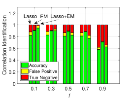
Figure 19: Correlation Identification Rate (Retail)

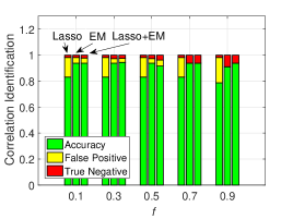
Figure 20: Correlation Identification Rate(Adult)

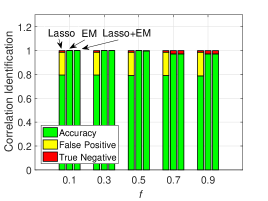
Figure 21: Correlation Identification Rate (TPC-E)

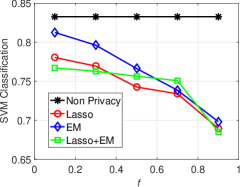
Figure 22: SVM Classification Rate (Retail)

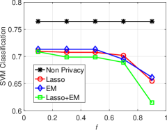
Figure 23: SVM Classification Rate (Adult)

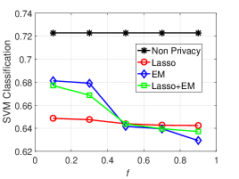
Figure 24: SVM Classification Rate (TPC-E)

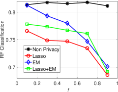
Figure 25: Random Forest Classification Rate (Retail)

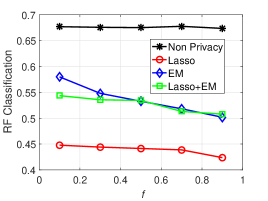
Figure 26: Random Forest Classification Rate (Adult)

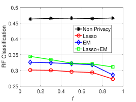
Figure 27: Random Forest Classification Rate (TPC-E)

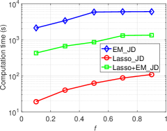
Figure 28: Overall Time of LoPub (Retail)

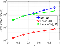
Figure 29: Overall Time of LoPub (Adult)

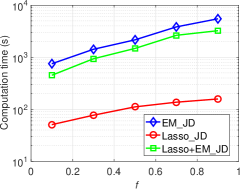
Figure 30: Overall Time of LoPub (TPC-E)

VII Conclusion

In this paper, we propose a novel solution, LoPub, to achieve the high-dimensional data release with local privacy in crowdsourced systems. Specifically, LoPub learns from the distributed data records to build the correlations and joint distribution of attributes, synthesizing an approximate dataset for privacy protection. To realise the effective multi-variate distribution estimation, we proposed EM-based and Lasso-based joint distribution estimation algorithms. The experiment results on the real datasets show that LoPub is an efficient and effective mechanism to release a high-dimensional dataset while providing sufficient local privacy guarantee for crowdsourced users.

References

- [1] Frequent itemset mining dataset. http://fimi.ua.ac.be/data/.
- [2] Trans. processing performance council. http://www.tpc.org/.
- [3] G. Acs, C. Castelluccia, and R. Chen. Differentially private histogram publishing through lossy compression. In Proc. of IEEE ICDM, pages 1–10, 2012.
- [4] M. Akg n, A. O. Bayrak, B. Ozer, and M. a. Sa??ro?lu. Privacy preserving processing of genomic data: A survey. Journal of Biomedical Informatics, 56:103–111, 2015.
- [5] K. Bache and M. Lichman. Uci machine learning repository. https://archive.ics.uci.edu/ml/datasets.html/, 2013.
- [6] R. Chen, H. Li, A. K. Qin, S. P. Kasiviswanathan, and H. Jin. Private spatial data aggregation in the local setting. In Proc. IEEE ICDE, pages 289–300, 2016.
- [7] R. Chen, Q. Xiao, Y. Zhang, and J. Xu. Differentially private high-dimensional data publication via sampling-based inference. In Proc. of ACM KDD, pages 129–138, 2015.
- [8] W. Day and N. Li. Differentially private publishing of high-dimensional data using sensitivity control. In Proc. of the ASIACCS, pages 451–462. ACM, 2015.
- [9] J. C. Duchi, M. I. Jordan, and M. J. Wainwright. Local privacy and statistical minimax rates. In Proc. of IEEE FOCS, pages 429–438, 2013.
- [10] C. Dwork. Differential privacy. In Proc. of ICALP, pages 1–12. 2006.
- [11] C. Dwork. Differential privacy: A survey of results. In Proc. Springer TAMC, pages 1–19. 2008.
- [12] C. Dwork, F. McSherry, K. Nissim, and A. Smith. Calibrating noise to sensitivity in private data analysis. Proc. of TCC, pages 265–284, 2006.
- [13] F. Eigner, A. Kate, M. Maffei, F. Pampaloni, and I. Pryvalov. Differentially private data aggregation with optimal utility. In Proceedings of the 30th Annual Computer Security Applications Conference, pages 316–325. ACM, 2014.
- [14] U. Erlingsson, V. Pihur, and A. Korolova. Rappor: Randomized aggregatable privacy-preserving ordinal response. In Proc. of ACM CCS, 2014.
- [15] L. Fan and L. Xiong. An adaptive approach to real-time aggregate monitoring with differential privacy. IEEE Trans. Knowl. Data Eng., 26(9):2094 – 2106, 2014.
- [16] G. Fanti, V. Pihur, and Ú. Erlingsson. Building a rappor with the unknown: Privacy-preserving learning of associations and data dictionaries. Proceedings on Privacy Enhancing Technologies, 2016(3):41–61, 2016.
- [17] M. M. Groat, B. Edwards, J. Horey, W. He, and S. Forrest. Enhancing privacy in participatory sensing applications with multidimensional data. In Proc. of IEEE PerCom, pages 144–152. IEEE, 2012.
- [18] N. Holohan, D. J. Leith, and O. Mason. Optimal differentially private mechanisms for randomised response. IEEE Trans. Inf. Forensics Security, 12(11):2726–2735, Nov 2017.
- [19] J. Hua, A. Tang, Y. Fang, Z. Shen, and S. Zhong. Privacy-preserving utility verification of the data published by non-interactive differentially private mechanisms. IEEE Trans. Inf. Forensics Security, 11(10):2298–2311, Oct 2016.
- [20] P. Kairouz, K. Bonawitz, and D. Ramage. Discrete distribution estimation under local privacy. arXiv preprint: 1602.07387, 2016.
- [21] P. Kairouz, S. Oh, and P. Viswanath. Extremal mechanisms for local differential privacy. In Proc. of NIPS, pages 2879–2887, 2014.
- [22] G. Kellaris and S. Papadopoulos. Practical differential privacy via grouping and smoothing. VLDB, 6(5):301–312, 2013.
- [23] W. Z. Khan, Y. Xiang, M. Y. Aalsalem, and Q. Arshad. Mobile phone sensing systems: A survey. IEEE Commun. Surveys Tuts., 15(1):402–427, 2013.
- [24] G. Li, J. Wang, Y. Zheng, and M. J. Franklin. Crowdsourced data management: A survey. IEEE Trans. Knowl. Data Eng., 28(9):2296–2319, 2016.
- [25] H. Li, L. Xiong, and X. Jiang. Differentially private synthesization of multi-dimensional data using copula functions. In Proc. EDBT, pages 475–486, 2014.
- [26] H. Li, L. Xiong, X. Jiang, and J. Liu. Differentially private histogram publication for dynamic datasets: an adaptive sampling approach. In Proc. of ACM CIKM, pages 1001–1010. ACM, 2015.
- [27] L. Li, R. Lu, K. K. R. Choo, A. Datta, and J. Shao. Privacy-preserving-outsourced association rule mining on vertically partitioned databases. IEEE Trans. Inf. Forensics Security, 11(8):1847–1861, Aug 2016.
- [28] N. Li, W. Qardaji, and D. Su. On sampling, anonymization, and differential privacy or, k-anonymization meets differential privacy. In Proc. of ACM ASIACCS, pages 32–33, 2012.
- [29] X. Liang, X. Li, R. Lu, X. Lin, and X. Shen. Udp: Usage-based dynamic pricing with privacy preservation for smart grid. IEEE Trans. Smart Grid, 4(1):141–150, 2013.
- [30] C. Liu, S. Chakraborty, and P. Mittal. Dependence makes you vulnerable: Differential privacy under dependent tuples. In Proc. of NDSS, 2016.
- [31] F. D. McSherry. Privacy integrated queries: an extensible platform for privacy-preserving data analysis. In Proc. of ACM SIGMOD, 2009.
- [32] M. Naveed, E. Ayday, E. W. Clayton, J. Fellay, C. A. Gunter, J. Hubaux, B. A. Malin, and X. Wang. Privacy in the genomic era. ACM Comput. Surv., 48(1):6, 2015.
- [33] N. Pham, R. K. Ganti, Y. S. Uddin, S. Nath, and T. Abdelzaher. Privacy-preserving reconstruction of multidimensional data maps in vehicular participatory sensing. In European Conference on Wireless Sensor Networks, pages 114–130. Springer, 2010.
- [34] W. Qardaji, W. Yang, and N. Li. Priview: practical differentially private release of marginal contingency tables. In Proc. of ACM SIGMOD, pages 1435–1446, 2014.
- [35] R. Sarathy and K. Muralidhar. Evaluating laplace noise addition to satisfy differential privacy for numeric data. Transactions on Data Privacy, 4(1):1–17, 2011.
- [36] H. Shen, M. Zhang, and J. Shen. Efficient privacy-preserving cube-data aggregation scheme for smart grids. IEEE Trans. Inf. Forensics Security, 12(6):1369–1381, 2017.
- [37] J. Soria-Comas, J. Domingo-Ferrer, D. S nchez, and D. Meg as. Individual differential privacy: A utility-preserving formulation of differential privacy guarantees. IEEE Trans. Inf. Forensics Security, 12(6):1418–1429, June 2017.
- [38] D. Starobinski, A. Trachtenberg, and S. Agarwal. Efficient pda synchronization. IEEE Trans. Mobile Comput., 2(1):40–51, 2003.
- [39] S. Su, P. Tang, X. Cheng, R. Chen, and Z. Wu. Differentially private multi-party high-dimensional data publishing. In Proc. of IEEE ICDE, pages 205–216, 2016.
- [40] J. Sun, R. Zhang, J. Zhang, and Y. Zhang. Pristream: Privacy-preserving distributed stream monitoring of thresholded percentile statistics. In Proc. of IEEE INFOCOM, pages 1–9, 2016.
- [41] R. Tibshirani. Regression shrinkage and selection via the lasso. Journal of the Royal Statistical Society. Series B (Methodological), pages 267–288, 1996.
- [42] Q. Wang, Y. Zhang, X. Lu, Z. Wang, Z. Qin, and K. Ren. Rescuedp: Real-time spatio-temporal crowd-sourced data publishing with differential privacy. In Proc. of IEEE INFOCOM, pages 1–9, 2016.
- [43] W. Wang and Q. Zhang. Privacy-preserving collaborative spectrum sensing with multiple service providers. IEEE Trans. Wireless Commun., 14(2):1011–1019, 2015.
- [44] S. L. Warner. Randomized Response: A Survey Technique for Eliminating Evasive Answer Bias. J. Am. Stat. Assoc., 60:63–69, 1965.
- [45] X. Yang, T. Wang, X. Ren, and W. Yu. Survey on improving data utility in differentially private sequential data publishing. IEEE Transactions on Big Data, PP(99):1–1, 2017.
- [46] J. Zhang, G. Cormode, C. M. Procopiuc, D. Srivastava, and X. Xiao. Privbayes: Private data release via bayesian networks. In Proc. of ACM SIGMOD, pages 1423–1434, 2014.
- [47] Y. Zhang, Q. Chen, and S. Zhong. Privacy-preserving data aggregation in mobile phone sensing. IEEE Trans. Inf. Forensics Security, 11(5):980–992, May 2016.
- [48] T. Zhu, P. Xiong, G. Li, and W. Zhou. Correlated differential privacy: Hiding information in non-iid data set. IEEE Trans. Inf. Forensics Security, 10(2):229–242, 2015.