Building Large Machine Reading-Comprehension Datasets using Paragraph Vectors

Abstract

We present a dual contribution to the task of machine reading-comprehension: a technique for creating large-sized machine-comprehension (MC) datasets using paragraph-vector models; and a novel, hybrid neural-network architecture that combines the representation power of recurrent neural networks with the discriminative power of fully-connected multi-layered networks. We use the MC-dataset generation technique to build a dataset of around 2 million examples, for which we empirically determine the high-ceiling of human performance (around 91% accuracy), as well as the performance of a variety of computer models. Among all the models we have experimented with, our hybrid neural-network architecture achieves the highest performance (83.2% accuracy). The remaining gap to the human-performance ceiling provides enough room for future model improvements.

1 Introduction

The ability to have computer models that can achieve genuine understanding of natural language text is a long-standing goal of Artificial Intelligence [Norvig, 1978]. The problem can be formulated in a relatively straight-forward manner, by borrowing the same techniques that are used for measuring reading comprehension in human students: given a text passage, measure how well they can answer questions related to the information being presented in that passage.

Previous attempts towards achieving this goal have ranged from hand-engineered grammars [Riloff and Thelen, 2000], to predicate-argument extraction and querying [Poon et al., 2010], to exploiting recently-proposed reading-comprehension datasets [Richardson et al., 2013, Berant et al., 2014, Hermann et al., 2015, Rajpurkar et al., 2016] using various machine learning approaches [Wang et al., 2015, Yin et al., 2016, Chen et al., 2016, Sordoni et al., 2016]. To better understand the current state of affairs in this field, let us take a look at two publicly-available reading-comprehension datasets and recap the current state-of-the-art (SOTA) results.

The MCTest [Richardson et al., 2013] contains about 500 stories associated with 2000 questions (4 questions per story), and 4 choices per question (only one correct); the stories and questions are written at the reading-level of elementary-school students (e.g., “James the Turtle was always getting in trouble.”). The human-level performance on this dataset is estimated to be in the high 90% range. The SOTA on this dataset is about 70% accuracy [Wang et al., 2015], obtained using a model that combines both traditional and more recent language-understanding tools, such as syntax, frame semantics, co-reference, and word embeddings. It’s worth noting here that models using various neural-network architectures achieve only about 53% accuracy [Yin et al., 2016], presumably because the small data size does not allow for optimal parameter estimation.

At the other end of the spectrum is the CNN/DailyMail dataset [Hermann et al., 2015], which is based on news articles from CNN and DailyMail; the number of examples are in the hundreds of thousands, and the reading-level of these text is high-school/college level; the ’questions’ are created from the bullet-point summaries that accompany these articles, and a clever entity-anonimization technique is used to ensure that only the information from the current passage is used to provide the answer (e.g., “According to the sci-fi website @entity9 , the upcoming novel @entity11 will feature a capable but flawed @entity13 official …”). On these datasets, the human-level performance is estimated to be around 75% accuracy [Chen et al., 2016], while the SOTA is currently at 76.1 on CNN [Sordoni et al., 2016], and 75.8 on DailyMail [Chen et al., 2016].

Consistent with the last research findings in a variety of natural-language tasks for which enough supervised training data is available, the SOTA results are achieved using neural-network models. For instance, the results in [Chen et al., 2016] are achieved using a neural-network architecture based on the AttentiveReader model originally proposed by [Hermann et al., 2015], together with some modifications that prove effective for the task. But since SOTA and human accuracy are so close for the CNN/DailyMail dataset, we conclude that it has fulfilled its mission and is now headed towards retirement (at least in the current form as a machine-comprehension dataset; see [Nallapati et al., 2016] for a useful reincarnation in the context of abstractive summarization).

In this context, we present a dual contribution to the field of Machine Comprehension of text. First, we present a technique via which one can obtain machine-comprehension datasets based on widely-available news data (e.g., the English Gigaword [Graff and Cieri, 2003]); we use this technique to generate a datasets of around 2 million examples, on which we estimate that the human-level accuracy is in the 90% range (in a 5-way multi-choice setup; for comparison, a random-guess approach has 20% accuracy). Second, we present a novel neural-network architecture that combines the representation power of recurrent neural networks with the discriminative power of fully-connected multi-layered networks, and achieves the best results we could obtain on our dataset: 83.2% accuracy.

These contributions open the doors for building interesting challenges for the Machine Comprehension task, along the following dimensions: we build such datasets over text that uses rich language constructs on both the input side (hence a requirement for understanding the context) and the output side (hence a need for understanding the answers), thus capturing a large spectrum of natural language understanding challenges; the large size of such datasets allows for exploring the performance of machine-learning models in a supervised-learning setting, including data-hungry models such as deep neural-network architectures; last but not least, we can use the difference between the human-performance ceiling on these datasets and the current SOTA to assess the progress made in the field of Machine Comprehension of text. We release the machine-comprehension dataset used in this paper to the research community, in order to facilitate direct comparisons against the results reported in this paper, as well as boost the influx of new contributions to the field.

2 Building a Paragraph-Vector–based MC Dataset

In this section, we describe an algorithm for the creation of Machine Comprehension datasets, based on exploiting Paragraph Vector [Le and Mikolov, 2014] models. The data requirement is that of a large set $C$ of $\langle\mbox{\it title},\mbox{\it article}\rangle$ pairs, of the type that can be extracted from a variety of publicly-available corpora, for instance the English Gigaword [Graff and Cieri, 2003].

2.1 The MC-Create Algorithm

The pseudo-code for the creation of the dataset is presented below:

Result: Dataset MC_C

Train paragraph-vector model $\textsf{PV}_{C}$

MC_C$\leftarrow\emptyset$

$nr\_decoys=4$

for $\langle\operatorname{\mathbf{t}},\operatorname{\mathbf{a}}\rangle\in C$ do

       $A\leftarrow[]$

       $T_{t}\leftarrow\mbox{\it PV}_{C}(\operatorname{\mathbf{t}})[1..N]$

       for $\operatorname{\mathbf{t}^{\prime}}\in T_{t}$ do

             $score\leftarrow Score(\operatorname{\mathbf{t}^{\prime}},\langle\operatorname{\mathbf{t}},\operatorname{\mathbf{a}}\rangle)$

             if $score>0$ then

                   $A.\mbox{\bf append}(\langle score,\operatorname{\mathbf{t}^{\prime}}\rangle)$

             end if

            

       end for

      if $|A|\geq nr\_decoys$ then

             MC_C$\leftarrow$ MC_C$\cup\{(\langle\operatorname{\mathbf{t}},\operatorname{\mathbf{a}}\rangle,\mbox{\bf true})\}$

             $R\leftarrow\mbox{\bf descending-sort}(A)$

             for $i\in[1..nr\_decoys]$ do

                   $\langle score,\operatorname{\mathbf{t}^{\prime}}\rangle\leftarrow R[i]$

                   MC_C$\leftarrow$ MC_C$\cup\{(\langle\operatorname{\mathbf{t}^{\prime}},\operatorname{\mathbf{a}}\rangle,\mbox{\bf false})\}$

                  

             end for

            

       end if

      

end for

Algorithm 1 MC-Create($C$, $N$, Score)

Algorithm MC-Create takes three main parameters: a dataset $C=\{\langle\operatorname{\mathbf{t}}_{i},\operatorname{\mathbf{a}}_{i}\rangle|1\leq i\leq m\}$; an integer $N$ that controls the paragraph-vector neighborhood size; and a function Score, used to score the $N$ entries for each such neighborhood.

The first step of the algorithm involves training a paragraph-vector model using the title entries in dataset $C$. For a given title $\operatorname{\mathbf{t}}$ in $C$, its $N$ closest neighbors in $PV_{C}$ are denoted $T_{t}$. Each title entry $\operatorname{\mathbf{t}^{\prime}}$ in $T_{t}$ is scored against the $\langle\operatorname{\mathbf{t}},\operatorname{\mathbf{a}}\rangle$ pair according to the Score function. In what follows, we are using the following Score function definition:

$$\textsf{Score}(\operatorname{\mathbf{t}^{\prime}},\langle\operatorname{\mathbf{t}},\operatorname{\mathbf{a}}\rangle)=\left\{\begin{array}[]{rl}0,&{\scriptstyle\mbox{if}\,\textsf{sim}_{\textsc{surf}}(\operatorname{\mathbf{t}^{\prime}},\operatorname{\mathbf{t}})\geq L}\\ \lambda_{e}\textsf{sim}_{\textsc{PV}}(\operatorname{\mathbf{t}^{\prime}},\operatorname{\mathbf{t}})&\\ +\lambda_{s}\textsf{sim}_{\textsc{surf}}(\operatorname{\mathbf{t}^{\prime}},\operatorname{\mathbf{t}})&{\scriptstyle\mbox{otherwise}}\\ +(1-\lambda_{s})\textsf{sim}_{\textsc{surf}}(\operatorname{\mathbf{t}^{\prime}},\operatorname{\mathbf{a}}))&\\ \end{array}\right.$$ (1)

This function uses the notation $\textsf{sim}_{\textsc{surf}}(\operatorname{\mathbf{t}^{\prime}},\operatorname{\mathbf{t}})$ to indicate a similarity score based on the surface of the strings $\operatorname{\mathbf{t}^{\prime}}$ and $\operatorname{\mathbf{t}}$, and $\textsf{sim}_{\textsc{PV}}(\operatorname{\mathbf{t}^{\prime}},\operatorname{\mathbf{t}})$ to indicate a similarity score based on the paragraph-vector representations of $\operatorname{\mathbf{t}^{\prime}}$ and $\operatorname{\mathbf{t}}$.

The Score function first verifies if the surface-based similarity for pair $\langle\operatorname{\mathbf{t}^{\prime}},\operatorname{\mathbf{t}}\rangle$ exceeds some threshold $L$. In that case, the function returns 0, as a guard against considering pairs that are too surface-similar; otherwise, it computes a weighted linear combination (using weights $\lambda_{e}$ and $\lambda_{s}$) between the embedding-based similarity $\textsf{sim}_{\textsc{PV}}(\operatorname{\mathbf{t}^{\prime}},\operatorname{\mathbf{t}})$ and the surface-based similarities $\textsf{sim}_{\textsc{surf}}$ for both $\langle\operatorname{\mathbf{t}^{\prime}},\operatorname{\mathbf{t}}\rangle$ and $\langle\operatorname{\mathbf{t}^{\prime}},\operatorname{\mathbf{a}}\rangle$. Intuitively, the higher this value is, the more likely it is that $\operatorname{\mathbf{t}^{\prime}}$ is a good decoy for $\operatorname{\mathbf{t}}$ with respect to article $\operatorname{\mathbf{a}}$.

For the dataset released with this paper and the experiments contained here, we used the following hyper-parameters: $\textsf{sim}_{\textsc{surf}}(\operatorname{\mathbf{t}^{\prime}},\operatorname{\mathbf{t}})$ is computed using BLEU [Papineni et al., 2002] (with brevity-penalty=1); $\textsf{sim}_{\textsc{PV}}(\operatorname{\mathbf{t}^{\prime}},\operatorname{\mathbf{t}})$ is computed as the cosine between the embedding representations PV$(\operatorname{\mathbf{t}^{\prime}})$ and PV$(\operatorname{\mathbf{t}})$; $\lambda_{e}$ = 1; $\lambda_{s}$ = 0.5; $L=0.5$; the paragraph-vector model PV_C is trained using the PV-DBOW model [Le and Mikolov, 2014] using softmax sampling, for 5 epochs with a token minimum count of 5, and an embedding size of 256.

Stats	Train	Dev	Test
#Instances	1,727,423	7,602	7,593
Avg. tokens/article	93.7	96.4	96.8
Avg. tokens/answer	9.6	9.9	9.9

Table 1: Statistics over the dataset created by MC-Create over the AFP portion of the Gigaword.

Article	Options
Two elite Australian air-force pilots were suspended for	1. Australian pilots suspended over landing gear miss: officials
going out drinking the night before they were were due to	2. Cambodian PM’s nephew cleared over fatal shootings, released
fly Prime Minister Julia Gillard, the defence department	3. Britain to hand over Basra in two weeks: PM’s office
said on Friday. The two members of the Royal Australian	4. Aussie PM’s pilots suspended over drinking spree
Air Force’s 34 Squadron were temporarily suspended but	5. Foreign media in a tangle over Spanish PM’s name
not disciplined further after the incident, the department
said.
Israeli Foreign Minister Avigdor Lieberman’s UN General	1. Climate czar’s departure will not impact talks: UN official
Assembly speech, which outlined controversial proposals	2. Iraq ”doesn’t understand” UN demands: Powell
for an Israeli-Palestinian agreement, did not reflect the	3. Israeli FM to hold talks with Rice, UN chief Annan on trip to US
official Israeli position, the premier’s office said Tuesday.	4. Lieberman UN speech doesn’t reflect Israel view on talks: PM
Prime Minister Benjamin Netanyahu appeared to be distan-	5. Syria ”not pessimistic” on peace with Israel: Assad
cing himself from Lieberman’s more controversial proposals.
The United States is pushing for peace talks between	1. Israel, Syria not ready for peace talks: US envoy
Israel, Syria and Lebanon, US envoy George Mitchell	2. Israel, Syria to resume stalled peace talks: US
said Tuesday, as the Israelis prepared to resume	3. Israel, Syria want to resume peace talks: US
direct negotiations with the Palestinians.	4. Lebanon, Syria discuss peace talks with Israel
	5. US seeks Israeli peace talks with Syria, Lebanon: envoy

Table 2: Examples of MC instances created by MC-Create over the AFP portion of the Gigaword.

	Dev dataset (sample)
	Difficulty			Accuracy
Method	Easy	Medium	Hard	Easy	Medium	Hard	Overall
Human	81%	14%	5%	93.6	86.4	57.1	90.9
BLEU (brev-penalty=1)				55.9	38.2	38.9	51.0
Paragraph-Vectors				16.8	14.7	5.6	15.0
Random				19.6	20.6	16.7	19.5

Table 3: Performance range for human and baseline methods on the AFP machine comprehension task.

2.2 Examples and Performance Range

We use the procedure described in Section 2.1 to generate a machine-comprehension dataset, using as $C$ the portion of the Gigaword corpus [Graff and Cieri, 2003] restricted to articles published by AFP (Agence France-Presse). The reason we restrict to one publisher has to do with information overlap: for a given news event, multiple publishers write headline & article pairs on that event, often to the extent that a headline from publisher A can fit perfectly an article from publisher B. Since this effect would muddle the one-correct-answer assumption for our dataset, we therefore recommend restricting the news corpus used to one publisher. The same effect can exist, to a smaller extent, even for a one-publisher corpus; we mitigate against it at a surface level, using threshold $L$ in the Score function (Equation 1) used by the MC-Create algorithm. We also note here that the size of set $C$ plays an important role in the creation of a challenging dataset; in our experience, it needs to be on the order of a few million examples, with smaller set sizes resulting in less challenging datasets.

The performance metric for such a dataset is straightforward: we compute accuracy by comparing the extent to which, when presented with an entry $E=\{\langle\operatorname{\mathbf{t}}_{i}^{j},\operatorname{\mathbf{a}}_{i}\rangle|1\leq j\leq 5\}$, the choice for index $j^{*}$, $1\leq j^{*}\leq 5$, coincides with having $(\langle\operatorname{\mathbf{t}}_{i}^{j^{*}},\operatorname{\mathbf{a}}_{i}\rangle,\mbox{\bf true})$ in MC_C.

We denote the MC dataset resulted from restricting to the AFP portion of the Gigaword as the MC${}_{\textsc{AFP}}\;$set. This dataset, including the train/dev/test splits used in the experiments reported in Section 4, is available online. (Note that you still need to have access to LDC’s English Gigaword Fifth Edition corpus [Graff and Cieri, 2003], in order to be able to generate the MC${}_{\textsc{AFP}}\;$dataset.) In Table 1 we present some statistics over the train/dev/test splits for the MC${}_{\textsc{AFP}}\;$set. Table 2 contains examples extracted from this dataset.

When considering the examples in Table 2, we note that the ’Article’ and ’Options’ columns illustrate a large spectrum of natural language understanding challenges: from simple lexical matching (e.g., ’PM’ and ’Prime Minister’), to complex lexicon usage (e.g., ’drinking spree’), to who-did-what-to-whom type of relationship determination. Our conjecture is that solving the challenge posed by such a dataset requires sophisticated language-understanding mechanisms.

To that end, we evaluate the performance of human annotators, as well as baseline algorithms, on a sample of size 200 extracted from this dataset, see Table 3. The human evaluators were asked, in addition to providing their best guess for the correct choice, to subjectively assess whether they perceived each example as ’Easy’, ’Medium’, or ’Hard’. For instance, the first example in Table 2 was annotated as ’Easy’, the second example ’Medium’, and the last example ’Hard’. It is interesting to note that the human accuracy scores accurately reflect this subjective difficulty assessment (first row in Table 3), with ’Easy’ examples averaging 93.6% accuracy, ’Medium’ at 86.4%, and ’Hard’ at 57.1%, for an overall performance of the human evaluator at 90.9% accuracy.

The surface-based baseline BLEU (brevity-penalty=1) chooses the maximum-scoring option using the BLEU [Papineni et al., 2002] metric. Its overall accuracy on this sample is 51.0%. This metric’s accuracy when considering the human-created labels of ’Easy’, ’Medium’, and ’Hard’ also reflects the fact that perceived difficulty correlates with surface string matching, with ’Easy’ examples averaging 55.9% accuracy, while ’Medium’ and ’Hard’ ones averaging around 38% accuracy.

The other non-trivial metric, Paragraph-Vectors, chooses the maximum-scoring option as the maximum cosine score between the article and each option. Because of its high correlation with how Algorithm MC-Create computes the decoy options, its performance at 15% accuracy is actually below that of random guessing (19.5% on this sample, expected to be 20% due to the 5 choices involved).

3 Neural Network–based MC Models

In this section, we present several neural-network–based models that we use to tackle the challenge presented by MC${}_{\textsc{AFP}}\;$. We use the following notations to describe these models: each training instance pair is a tuple $\langle\operatorname{\mathbf{t}}_{i},\operatorname{\mathbf{a}}_{i}^{j}\rangle$, where $\operatorname{\mathbf{a}}_{i}$ denotes the article, and $\operatorname{\mathbf{t}}_{i}^{j}$ denotes the title option; in addition, we use a binary variable $y_{ijk}\in\{0,1\}$ to denote whether the $j$-th title of instance $i$ is labeled as $k$, and $\sum_{k}y_{ijk}=1$.

3.1 Feedforward Neural Network Models

We experiment with the ability of standard feedforward neural-network models to solve the MC${}_{\textsc{AFP}}\;$task.

We consider two types of classifiers. A 2-class–classifier (1 for ’yes’, this is a correct answer; 0 for ’no’, this is an incorrect answer) applied independently on all $\langle\operatorname{\mathbf{t}}_{i},\operatorname{\mathbf{a}}_{i}^{j}\rangle$ pairs; the final prediction is the title with the highest ’yes’ probability among all instance pairs belonging to instance $i$.

For each instance pair $\langle\operatorname{\mathbf{t}}_{i},\operatorname{\mathbf{a}}_{i}^{j}\rangle$, the input to the neural network is an embedding tuple $\langle\text{Emb}(\operatorname{\mathbf{a}}_{i};\Omega),\text{Emb}(\operatorname{\mathbf{t}}_{i}^{j};\Omega)\rangle$, where $\Omega$ is the embedding matrix, and $\text{Emb}(.)$ denotes the mapping from a list of word IDs to a list of embedding vectors using $\Omega$.

Using these notations, the loss function for an FFNN can be written as:

$$L(\Omega,\operatorname{\mathbf{u}})=\sum_{i,j,k}y_{ijk}\log\;\text{FN}_{k}(\text{Emb}(\operatorname{\mathbf{a}}_{i};\Omega),\text{Emb}(\operatorname{\mathbf{t}}_{i}^{j};\Omega);\operatorname{\mathbf{u}})$$ (2)

where $\text{FN}_{k}$ denotes the $k$-th output of a feedforward neural network, and $\sum_{k}\text{FN}_{k}(.)=1$. Our architecture uses a two hidden-layer fully connected network with Rectified Linear hidden units, and a softmax layer on top.

In addition, we also consider a multi-class classifier, where each class $k$ corresponds to the index of the answer choice. In this case, we slightly modify Eq. 2 by

$$L(\Omega,\operatorname{\mathbf{u}})=\sum_{i,k}y_{ik}\log\;\text{FN}_{k}(\text{Emb}(\operatorname{\mathbf{a}}_{i};\Omega),\text{Emb}(\operatorname{\mathbf{t}}_{i}^{:};\Omega);\operatorname{\mathbf{u}})$$

where $\operatorname{\mathbf{t}}_{i}^{:}=\left\{\operatorname{\mathbf{t}}_{i}^{1},\ldots,\operatorname{\mathbf{t}}_{i}^{5}\right\}$ is a concatenation of all 5 candidate titles of instance $i$.

3.2 Seq2seq + Feedforward Models

We describe here a novel, hybrid neural-network model that combines a recurrent neural-network with a feedforward one. We note that both strings in a tuple $\langle\operatorname{\mathbf{t}}_{i},\operatorname{\mathbf{a}}_{i}^{j}\rangle$ can be modeled as the encoding and decoding sequences of a sequence-to-sequence (Seq2seq) model [Sutskever et al., 2014, Bahdanau et al., 2015]. The output of each unit cell of a Seq2seq model (both on the encoding side and the decoding side) can be fed into an FFNN architecture for binary classification. See Figure 1 for an illustration of the Seq2seq + FFNN model architecture.

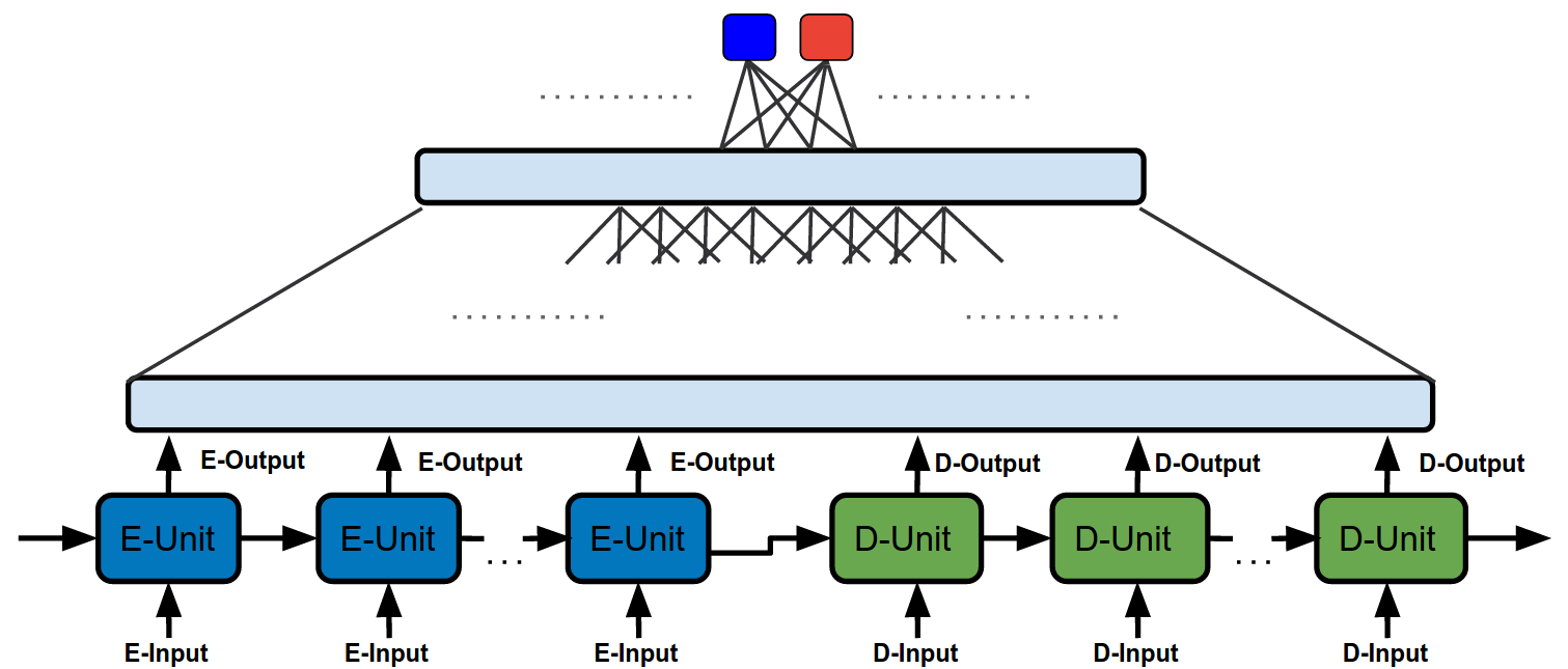
Figure 1: Seq2seq + FFNN model architecture.

In addition to the classification loss (Equation 2), we also include a loss for generating an output sequence $\operatorname{\mathbf{t}}_{i}^{j}$ based on an input $\operatorname{\mathbf{a}}_{i}$ sequence. We define a binary variable $z_{ijlv}\in\{0,1\}$ to indicate whether the $l$th word of $\operatorname{\mathbf{t}}_{i}^{j}$ is equal to word $v$. $\operatorname{\mathbf{O}}^{d}_{ijl}$ denotes the $l$-th output of the decoder of $\langle\operatorname{\mathbf{t}}_{i},\operatorname{\mathbf{a}}_{i}^{j}\rangle$, $\operatorname{\mathbf{O}}^{e}_{ij:}$ denotes the concatenation of all the output of the encoder of $\langle\operatorname{\mathbf{t}}_{i},\operatorname{\mathbf{a}}_{i}^{j}\rangle$, and $\operatorname{\mathbf{O}}^{d}_{ij:}$ denotes the concatenation of decoder outputs of $\langle\operatorname{\mathbf{t}}_{i},\operatorname{\mathbf{a}}_{i}^{j}\rangle$.

With these definitions, the loss function for the Seq2seq + FFNN model is:

$$L(\operatorname{\mathbf{\Theta}},\operatorname{\mathbf{w}},\operatorname{\mathbf{u}})=\sum_{i,j,k}y_{ijk}\log\;\text{FN}_{k}(\operatorname{\mathbf{O}}^{e}_{ij:}(\operatorname{\mathbf{a}}_{i},\operatorname{\mathbf{t}}_{i}^{j};\operatorname{\mathbf{\Theta}}),\operatorname{\mathbf{O}}^{d}_{ij:}(\operatorname{\mathbf{a}}_{i},\operatorname{\mathbf{t}}_{i}^{j};\operatorname{\mathbf{\Theta}});\operatorname{\mathbf{u}})+\lambda_{gen}\sum_{i,j,l,v}y_{ij1}z_{ijlv}\log\;\text{softmax}_{v}(\operatorname{\mathbf{O}}^{d}_{ijl}(\operatorname{\mathbf{a}}_{i},\operatorname{\mathbf{t}}_{i}^{j};\operatorname{\mathbf{\Theta}});\operatorname{\mathbf{w}})$$ (3)

where $\sum_{v}\text{softmax}_{v}(.)=1$; $\operatorname{\mathbf{\Theta}}$ are the parameters of the Seq2seq model, which include the parameters within each unit cell, as well as the elements in the embedding matrices for source and target sequences; $\operatorname{\mathbf{w}}$ are the output projection parameters that transform the output space of the decoder to the vocabulary space for abstract generation; $\operatorname{\mathbf{u}}$ are the parameters of the FFNN model (Equation 2); $\lambda_{gen}$ is the weight assigned to the sequence-to-sequence generation loss. Only the true target candidates (the ones with $y_{ij1}=1$) are included in this loss, as we do not want the decoy target options to affect this computation.

The Seq2seq model we use here is the attention-enhanced models proposed in [Bahdanau et al., 2015, Chen et al., 2016]. We apply Gated Recurrent Unit (GRU) as the unit cell [Cho et al., 2014]. For comparison purposes, the attention probabilistic mask $\alpha$ is instantiated using either the tanh layer as in [Bahdanau et al., 2015], or the bilinear term as in [Chen et al., 2016]. We also perform ablation tests to measure the impact on performance of the $\lambda_{gen}$ parameter in Section 4.3.1, and ablation tests to compare the performance of tied/untied embedding matrix for encoding and decoding sequences in Section 4.3.2.

4 Experiments

4.1 Experimental Setup

The experiments with neural network models are done using the Tensorflow package [Abadi et al., 2015]. The hyper-parameter choices are decided using the hold-out development portion of the MC${}_{\textsc{AFP}}\;$set. For modeling the input tokens, we use a vocabulary size of 100,000 types (selected as the most frequent tokens over the titles of the AFP portion of the English Gigaword corpus [Graff and Cieri, 2003]), with an embedding size of 512. The models are optimized using ADAGRAD with a learning rate of 0.01, and clipped gradients (maximum norm 4). We run the training procedure for 1M steps, with a mini-batch size of 200. We use 40 workers for computing the updates, and 10 parameter servers for model storing and (asynchronous and distributed) updating.

We use the following notations to refer to the neural network models: FFNN${}_{\mbox{5-class}}\;$refers to a feedforward neural network architecture with a 5-class–classifier, each class corresponding to an answer choice; we also refer to this model as FFNN5. FFNN${}_{\mbox{2-class}}^{\mbox{argmax 1..5}}\;$refers to a feedforward neural network architecture with a 2-class–classifier (’yes’ or ’no’ for answer correctness), over which an argmax function computes a 5-way decision (i.e., the choice with the highest ’yes’ probability); we henceforth refer to this model simply as FFNN. Both models use a two-hidden–layer architecture with sizes 1024 and 256.

The Seq2seq+FFNN refers to the hybrid model described in Section 3.2, in which the Seq2seq model is combined with the FFNN${}_{\mbox{2-class}}^{\mbox{argmax 1..5}}\;$model. The RNN part of the model uses a two-hidden–layer GRU unit-cell configuration, while the FFNN part uses a two-hidden–layer architecture with sizes 64 and 16. (We note here that for the hybrid model we also tried a larger FFNN setup with hidden layers of sizes 1024 and 256, but did not see improvements.)

The $\lambda_{gen}$ hyper-parameter from the loss-function $L(\operatorname{\mathbf{\Theta}},\operatorname{\mathbf{w}},\operatorname{\mathbf{u}})$ (Equation 3) is by default set to 0.01 (except for Section 4.3.1 where we directly measure its effect on performance). The embedding matrices for encoding and decoding sequences are tied together, and the attention mask $\alpha$ is computed using a bilinear term [Chen et al., 2016]. More extensive comparisons regarding the hyper-parameter choices are presented in Section 4.3.

4.2 Experimental Results

We first report the results of the main neural-network models we consider, against random-choice and surface-based baselines, see Table 4.

For a given hyper-parameter configuration, the neural-network model starts from a random parameter initialization, and updates its parameters using the training set for a maximum of 1 million steps. We monitor the classification accuracies on the dev set and select the checkpoint with the optimal performance on the dev set. The selected checkpoint is then evaluated on the test set. The reported error bars on the test set are estimated based on the standard deviation of the posterior distribution of the balanced accuracy [Brodersen et al., 2010].

Method	Dev	Test
Random-choice	19.5	20.2
BLEU (brev-penalty=1)	41.9	42.2
Paragraph-Vectors	16.1	17.4
FFNN5	57.8	58.1 $\pm$ 0.5
FFNN	72.8	72.5 $\pm$ 0.4
Seq2seq+FFNN	83.5	83.2 $\pm$ 0.4

Table 4: Classification accuracy on the MC${}_{\textsc{AFP}}\;$task for baselines and NN models.

The results clearly indicate the superiority of the neural-network models over the baselines. In addition, the 5-way direct classification done by FFNN5 is inferior to a 2-way classification approach followed by an argmax operation, a result somewhat surprising considering that the FFNN5 model has the benefit of more information available at both train- and run-time.

The Seq2seq+FFNN model obtains the best results, with accuracies of 83.5% (dev) and 83.2% (test); this performance indicates that this architecture is superior to any of the non-recurrent ones, and establishes a high-bar for a computer model performance on the MC${}_{\textsc{AFP}}\;$task. According to the results from Table 3, this level of performance is still below the  90% accuracy achievable by humans, which makes MC${}_{\textsc{AFP}}\;$an interesting challenge for future Machine Comprehension models.

In Table 9, we provide examples of instances that span the spectrum from easy to hard, according to the accuracy obtained by increasingly more competitive learning approaches. Next, we show the impact on performance of some of the decisions that we made regarding the models and the training procedure.

4.2.1 Order of training examples

We compare the results between training our NN models on the organized training set of MC${}_{\textsc{AFP}}\;$(e.g., with data fed to the model in the ’normal’ order $\langle\operatorname{\mathbf{t}}_{i}^{1},\operatorname{\mathbf{a}}_{i}\rangle,\langle\operatorname{\mathbf{t}}_{i}^{2},\operatorname{\mathbf{a}}_{i}\rangle,\ldots,\langle\operatorname{\mathbf{t}}_{h}^{1},\operatorname{\mathbf{a}}_{h}\rangle,\langle\operatorname{\mathbf{t}}_{h}^{2},\operatorname{\mathbf{a}}_{h}\rangle,\ldots$), compared to a dataset with the tuples randomly shuffled (e.g., with data of the form $\langle\operatorname{\mathbf{t}}_{i}^{1},\operatorname{\mathbf{a}}_{i}\rangle,\ldots,\langle\operatorname{\mathbf{t}}_{h}^{2},\operatorname{\mathbf{a}}_{h}\rangle,\ldots,\langle\operatorname{\mathbf{t}}_{i}^{2},\operatorname{\mathbf{a}}_{i}\rangle,\ldots,\langle\operatorname{\mathbf{t}}_{h}^{1},\operatorname{\mathbf{a}}_{h}\rangle,\ldots$). Results for this comparison are shown in Table 5.

Method	Shuffled	Dev	Test
FFNN	no	70.5	70.2 $\pm$ 0.4
FFNN	yes	72.8	72.5 $\pm$ 0.4
Seq2seq+FFNN	no	80.4	79.4 $\pm$ 0.4
Seq2seq+FFNN	yes	83.5	83.2 $\pm$ 0.4

Table 5: The impact of dataset-shuffling on MC${}_{\textsc{AFP}}\;$accuracy.

We see that for both models, the randomly-shuffled dataset performs better than the organized dataset. The results seem to indicate that our models have their parameters tuned better when the training signal is not presented in contiguous chunks (five binary decisions about a given $\operatorname{\mathbf{a}}_{i}$), and instead is presented as independent binary decisions for various $\operatorname{\mathbf{a}}_{i}$ and $\operatorname{\mathbf{a}}_{h}$s.

4.2.2 Difficulty of training examples

We also wanted to understand the extent to which the difficulty of the decoy answers influences the model’s ability to solve the MC${}_{\textsc{AFP}}\;$task. More precisely, we want to answer these two questions: is using ’difficult’ decoy answers always the best strategy when training such an MC model? would a model trained on both ’easy’ and ’difficult’ decoys converge to a better optimum?

To that end, we also created an additional dataset where the decoy targets are easier: the four decoy targets for a specific source $\operatorname{\mathbf{a}}_{i}$ are chosen randomly from the candidate targets for all sources. Let us denote this version of the dataset as MC${}_{\textsc{AFP}}^{\mbox{Rnd}}\;$. We keep constant the dev and test splits for MC${}_{\textsc{AFP}}\;$, and allow the training dataset to be produced as MC${}_{\textsc{AFP}}\;$, MC${}_{\textsc{AFP}}^{\mbox{Rnd}}\;$, as well as a combination of both (with one true and eight decoy answers). The results of using these setups are shown in Table 6.

Method	Train	Dev	Test
FFNN	MC${}_{\textsc{AFP}}\;$	72.8	72.5 $\pm$ 0.4
FFNN	MC${}_{\textsc{AFP}}^{\mbox{Rnd}}\;$	62.0	61.0 $\pm$ 0.5
FFNN	MC${}_{\textsc{AFP}}\;$+ MC${}_{\textsc{AFP}}^{\mbox{Rnd}}\;$	75.5	75.8 $\pm$ 0.4
Seq2seq+FFNN	MC${}_{\textsc{AFP}}\;$	83.5	83.2 $\pm$ 0.4
Seq2seq+FFNN	MC${}_{\textsc{AFP}}^{\mbox{Rnd}}\;$	73.1	73.3 $\pm$ 0.4
Seq2seq+FFNN	MC${}_{\textsc{AFP}}\;$+ MC${}_{\textsc{AFP}}^{\mbox{Rnd}}\;$	81.8	81.4 $\pm$ 0.4

Table 6: The impact of training-example–difficulty on MC${}_{\textsc{AFP}}\;$accuracy.

The results indicate that indeed, for certain NN architectures such as FFNN, the models can get significantly better by learning from both ’easy’ and ’difficult’ examples (75.8 on test, versus 72.5 on the same test set but using only ’difficult’ examples in training). Since we keep fixed the dev and test datasets to the ones from MC${}_{\textsc{AFP}}\;$, it is interesting to see the FFNN model benefit from being trained on a dataset with a different distribution than the one on which is being tested.

This effect, however, is not observed for the Seq2seq+FFNN model. This model does not benefit from training on ’easy’ examples, and the model resulting from training on MC${}_{\textsc{AFP}}\;$+ MC${}_{\textsc{AFP}}^{\mbox{Rnd}}\;$has an accuracy level of 81.4 (test) that is statistically-significant lower than the best result of 83.2 (test).

4.3 Hyper-parameters for Seq2seq+FFNN 

In this section, we investigate the effect of various hyper-parameter settings on the performance of the Seq2seq+FFNN model.

4.3.1 Effect of $\lambda_{gen}$

We compare models with different values of $\lambda_{gen}$, affecting the loss-function $L(\operatorname{\mathbf{\Theta}},\operatorname{\mathbf{w}},\operatorname{\mathbf{u}})$ defined in Equation 3. As we can see from Table 7, lower $\lambda_{gen}$ values lead to higher MC accuracy scores. This observation agrees with the intuition that training the model using a loss $L(\operatorname{\mathbf{\Theta}},\operatorname{\mathbf{w}},\operatorname{\mathbf{u}})$ with larger $\lambda_{gen}$ means the MC loss (the first term of the loss) may get overwhelmed by the word-generation loss (the second term). On the other hand, higher $\lambda_{gen}$ values trigger an increase in performance associated with the generation task, as measured by the ROUGE-L [Lin and Och, 2004] score between the generated answer and the ground-truth answer (last column in Table 7).

$\lambda_{gen}$	Dev	Test	ROUGE-L
0.0	83.2	82.7 $\pm$ 0.4	0.1
0.01	83.5	83.2 $\pm$ 0.4	0.7
0.1	82.8	83.0 $\pm$ 0.4	11.4
0.5	82.8	82.3 $\pm$ 0.4	27.7
1.0	76.9	76.4 $\pm$ 0.4	27.9
2.0	78.1	77.3 $\pm$ 0.4	33.2
5.0	79.3	78.7 $\pm$ 0.4	34.5
10.0	75.0	74.2 $\pm$ 0.4	35.1

Table 7: The impact of $\lambda_{gen}$ on MC${}_{\textsc{AFP}}\;$accuracy (as well as generation accuracy).

The conclusion we derive from the results in Table 7 is that the Seq2seq+FFNN model is capable of tuning both its encoding and decoding mechanisms according to the loss, which directly translates into the corresponding level of MC accuracy. For $\lambda_{gen}=0.01$, the loss favors directly the classification task, resulting on high accuracy on both dev (83.5) and test (83.2). On the other hand, a setting like $\lambda_{gen}=5.0$ gives a reasonable MC accuracy (78.7 on test, significantly higher than the best obtained by any FFNN model), while also producing high-scoring abstractive answers (34.5 ROUGE-L score). This is akin to a situation in which a student makes a multiple-choice decision by also producing, in addition to an answer choice 1-5, their own original answer. For instance, for the last example in Table 2, this model generates from the ’Article’ entry the following abstractive answer: ’US envoy says Israel-Syria peace talks to resume.’

4.3.2 Effect of tied-embeddings and bilinear-attention

We also compare the impact on the MC accuracy for the Seq2seq+FFNN model of several choices regarding the embedding matrices, as well as the implementation of the attention model. The results are shown in Table 8 (using a fixed $\lambda_{gen}=0.01$).

Tied-Embeddings	Bilinear-Attn	Dev	Test
no	no	70.7	70.2 $\pm$ 0.4
yes	no	75.7	74.6 $\pm$ 0.4
no	yes	77.9	77.1 $\pm$ 0.4
yes	yes	83.5	83.2 $\pm$ 0.4

Table 8: The impact of tied-embeddings and bilinear attention on the Seq2seq+FFNN model.

The results indicate that tied embeddings have a net positive effect: it reduces the number of model parameters by nearly half, while also contributing between 4 and 6 absolute points in accuracy. The mechanism of bilinear attention [Chen et al., 2016] is also superior to the one using only a tanh layer [Bahdanau et al., 2015], by influencing the decoder outputs such that the loss favoring classification accuracy ($\lambda_{gen}=0.01$) is minimized. It contributes about 5 absolute accuracy-points, in a manner that is orthogonal with the contribution of the tied-embeddings, for a high-water–mark of 83.2% accuracy on the MC${}_{\textsc{AFP}}\;$test set.

5 Conclusion

The task of making machine truly comprehend written text is far from solved. To make meaningful progress, we need to attack the problem on two different fronts: build high-quality, high-volume datasets for training and testing machine-comprehension models; and, given the full complexity of natural language [Winograd, 1972], invent comprehension models that can be trained to perform well on this task.

This paper presents contributions on each of these fronts. The algorithm presented in Section 2.1, MC-Create, can be used to create datasets that are both high quality and high volume, starting from data that appears naturally in today’s world (e.g., news). Since the method presented is language-agnostic, it can also be used to create MC datasets in languages other than English, a promising prospect. Regarding models of comprehension, the proposed hybrid Seq2seq+FFNN model not only performs at a high-level on the MC${}_{\textsc{AFP}}\;$dataset, but has the potential to tackle a lot of other tasks that present both a generation and a discrimination component. Such advances in the machine-comprehension task have the potential to move the field forward in the pursuit of genuine understanding of natural language by computers.

Correct	Incorrect
BLEU (brev-penalty=1)
The vice-mayor of Beijing in charge of traffic management	Somali pirates on Saturday captured a Thai bulk carrier with
has resigned and been sent to the far-western region of	its 27 crew members in the Arabian Sea, a maritime official
Xinjiang as officials take drastic steps to ease chronic gridlock	said. The Thor Nexus was seized in the early hours while on
in the Chinese capital. Huang Wei’s resignation and	its way to Bangladesh from the United Arab Emirates. All its
appointment as vice-chairman of Xinjiang were approved	crew members are Thai, said Andrew Mwangura of the East
Thursday, the official Xinhua news agency said – the same day	African Seafarers Assistance Programme.
Beijing announced plans to slash the number of new cars in
the city next year.
1. Argentine official resigns amid economic crisis	1. Somali pirates seize Panama freighter: official
2. Beijing traffic official resigns amid gridlock woes	2. Somali pirates seize Spanish fishing boat: maritime official
3. Italian PM Berlusconi’s party in crisis as top official resigns	3. Somali pirates seize Thai fishing vessels, 77 crew: EU force
4. Sri Lanka budget raises fears of inflation, top official	4. Somali pirates seize Thai vessel, 27 crewmen: official
resigns	5. Somali pirates seize two more cargo vessels: official
5. Top Dhaka University official resigns amid fresh campus
violence
Seq2seq+FFNN
Yemen has deployed new anti-terrorism forces in the country’s	As almost round-the-clock night descends on their country in
restive south, the ministry of interior announced Saturday, as	December, Swedes turn to an informal celebration of light,
Washington urged Sanaa to step up its fight against	in keeping with long-running traditions and an effort to cope
Al-Qaeda. The announcement follows a spate of deadly attacks	with the darkest time of the year. Candles appear in the
on government and military targets in the south, the latest	windows of homes, shops, offices and cafes throughout Sweden
on Friday when according to a security official a suspected	from the start of Advent, on the fourth Sunday before
Al-Qaeda militant shot dead a soldier who ferried him on his	Christmas, to the end of December, when dusk can start
motorbike taxi in Zinjibar , capital of Abyan province.	creeping over Stockholm as early as 2:00pm.
1. Five nations to form anti-terrorism network	1. At the darkest time of year, Swedes make their own light
2. Iraq, Sudan, Libya join Arab anti-terrorism conference	2. Gebrselaisse runs best 1,500m time of year
3. Pakistani police to install 100 anti-terrorism surveillance	3. Making light work: The 50-year odyssey of the laser
cameras	4. RugbyU : Highlanders record their second win of the year
4. Yemen says US did not ask to participate in al-Qaeda hunt	5. Six-month-old girl, three-year-old boy tie the knot in Nepal
5. Yemen says anti-terrorism forces sent to south
Human Annotator
Organisers of South Korea’s first Formula One event say they	Pope Benedict XVI has stepped up his displays of contrition
are confident they can complete the brand-new circuit before	towards victims of paedophile priests on his state visit to
a final inspection from the sport’s world governing body.	Britain, but he still has far to go to win back public opinion,
India’s Karun Chandhok on Saturday became the first F1 driver	observers said. Benedict met five British abuse victims and
to test out the 5.6-kilometre (3.5-mile)track, which boasts Asia’s	expressed ”deep sorrow” during mass on Saturday, in the
longest straight stretch, and declared it basically in good shape.	latest of several attempts to tackle an issue that is
[…]	rocking the Catholic Church […].
1. Formula One: SKorea to build Asia’s longest track	1. Brazil’s indigenous people still victims of abuse: report
2. Formula One: India to hold F1 race in 2009	2. Pope’s Australia sex abuse apology not enough: critics
3. Formula One: Builders race to finish first S.Korea F1 track	3. Pope’s abuse scandal apologies still not enough: experts
4. Formula One: India to hold F1 race in 2010	4. Pope’s sex abuse apology not enough, some victims say
5. Formula One: S.Korea’s F1 track to be ready in late August	5. Vatican’s toughening of abuse rules is only a start: experts

Table 9: Examples from the dev set of the MC${}_{\textsc{AFP}}\;$dataset. The options in bold are the groundtruth answers, whereas the options in italics are the selected answers (by the respective methods). The left-side column shows cases where the respective methods got the correct answers, while the right-side column shows cases where the answers were incorrect.

References

- [Abadi et al., 2015] M. Abadi, A. Agarwal, P. Barham, E. Brevdo, Z. Chen, C. Citro, G. Corrado, A. Davis, J. Dean, M. Devin, S. Ghemawat, I. Goodfellow, A. Harp, G. Irving, M. Isard, Y. Jia, R. Jozefowicz, L. Kaiser, M. Kudlur, J. Levenberg, D. Mané, R. Monga, S. Moore, D. Murray, C. Olah, M. Schuster, J. Shlens, B. Steiner, I. Sutskever, K. Talwar, P. Tucker, V. Vanhoucke, V. Vasudevan, F. Viégas, O. Vinyals, P. Warden, M. Wattenberg, M. Wicke, Y. Yu, and X. Zheng. 2015. TensorFlow: Large-scale machine learning on heterogeneous systems. Software available from tensorflow.org.
- [Bahdanau et al., 2015] Dzmitry Bahdanau, Kyunghyun Cho, and Yoshua Bengio. 2015. Neural machine translation by jointly learning to align and translate. In Proceedings of ICLR.
- [Berant et al., 2014] Jonathan Berant, Vivek Srikumar, Pei-Chun Chen, Abby Vander Linden, Brittany Harding, Brad Huang, Peter Clark, and Christopher D. Manning. 2014. Modeling biological processes for reading comprehension. In Proceedings of EMNLP.
- [Brodersen et al., 2010] Kay Henning Brodersen, Cheng Soon Ong, Klaas Enno Stephan, and Joachim M. Buhmann. 2010. The balanced accuracy and its posterior distribution. In Proceedings of the 2010 20th International Conference on Pattern Recognition, pages 3121–3124.
- [Chen et al., 2016] Danqi Chen, Jason Bolton, and Christopher D. Manning. 2016. A Thorough Examination of the CNN/Daily Mail Reading Comprehension Task. In Proceedings of ACL.
- [Cho et al., 2014] Kyunghyun Cho, Bart van Merrienboer, Çaglar Gülçehre, Dzmitry Bahdanau, Fethi Bougares, Holger Schwenk, and Yoshua Bengio. 2014. Learning phrase representations using RNN encoder-decoder for statistical machine translation. In Proceedings of EMNLP, October 25-29, 2014, Doha, Qatar, pages 1724–1734.
- [Graff and Cieri, 2003] David Graff and Christopher Cieri. 2003. English gigaword fifth edition ldc2003t05. In Linguistic Data Consortium, Philadelphia.
- [Hermann et al., 2015] Karl Moritz Hermann, Tomáš Kočiský, Edward Grefenstette, Lasse Espeholt, Will Kay, Mustafa Suleyman, and Phil Blunsom. 2015. Teaching machines to read and comprehend. In Proceedings of NIPS.
- [Le and Mikolov, 2014] Quoc Le and Tomas Mikolov. 2014. Distributed representations of sentences and documents. In Proceedings of the 31st International Conference on Machine Learning, Beijing, China.
- [Lin and Och, 2004] Chin-Yew Lin and Franz Josef Och. 2004. Automatic evaluation of machine translation quality using longest common subsequence and skip-bigram statistics. In Proceedings of ACL.
- [Nallapati et al., 2016] R. Nallapati, B. Xiang, and B. Zhou. 2016. Sequence-to-sequence RNNs for text summarization. CoRR, abs/1602.06023.
- [Norvig, 1978] Peter Norvig. 1978. A Unified Theory of Inference for Text Understanding. Ph.D. thesis, University of California, Berkeley.
- [Papineni et al., 2002] Kishore Papineni, Salim Roukos, Todd Ward, and Wei-Jing Zhu. 2002. Bleu: A method for automatic evaluation of machine translation. In Proceedings of ACL, pages 311–318.
- [Poon et al., 2010] H. Poon, J. Christensen, P. Domingos, O. Etzioni, R. Hoffmann, C. Kiddon, T. Lin, X.o Ling, Mausam, A. Ritter, S. Schoenmackers, S. Soderland, D. Weld, F. Wu, and C. Zhang. 2010. Machine reading at the University of Washington. In Proceedings of the NAACL/HLT First International Workshop on Formalisms and Methodology for Learning by Reading.
- [Rajpurkar et al., 2016] Pranav Rajpurkar, Jian Zhang, Konstantin Lopyrev, and Percy Liang. 2016. Squad: 100,000+ questions for machine comprehension of text. In Proceedings of EMNLP.
- [Richardson et al., 2013] Matthew Richardson, Christopher J.C. Burges, and Erin Renshaw. 2013. MCTest: A challenge dataset for the open-domain machine comprehension of text. In Proceedings of EMNLP, pages 193––203, Seattle, Washington, USA.
- [Riloff and Thelen, 2000] Ellen Riloff and Michael Thelen. 2000. A rule-based question answering system for reading comprehension tests. In Proceedings of ANLP/NAACL-2000 Workshop on Reading Comprehension Tests as Evaluation for Computer-Based Language Understanding System.
- [Sordoni et al., 2016] Alessandro Sordoni, Phillip Bachman, and Yoshua Bengio. 2016. Iterative alternating neural attention for machine reading. CoRR, abs/1606.02245.
- [Sutskever et al., 2014] Ilya Sutskever, Oriol Vinyals, and Quoc V. V Le. 2014. Sequence to sequence learning with neural networks. In Advances in Neural Information Processing Systems 27, pages 3104–3112. Curran Associates, Inc.
- [Wang et al., 2015] Hai Wang, Mohit Bansal, Kevin Gimpel, and David McAllester. 2015. Machine comprehension with syntax, frames, and semantics. In Proceedings of ACL.
- [Winograd, 1972] Terry Winograd. 1972. Understanding Natural Language. Academic Press Inc., Orlando, FL, USA.
- [Yin et al., 2016] Wenpeng Yin, Sebastian Ebert, and Hinrich Schutze. 2016. Attention-based convolutional neural network for machine comprehension. In Proceedings of NAACL Human-Computer Question Answering Workshop.