A Qualitative and Quantitative Evaluation of
8 Clear Sky Models

Abstract

We provide a qualitative and quantitative evaluation of 8 clear sky models used in Computer Graphics. We compare the models with each other as well as with measurements and with a reference model from the physics community. After a short summary of the physics of the problem, we present the measurements and the reference model, and how we ”invert” it to get the model parameters. We then give an overview of each CG model, and detail its scope, its algorithmic complexity, and its results using the same parameters as in the reference model. We also compare the models with a perceptual study. Our quantitative results confirm that the less simplifications and approximations are used to solve the physical equations, the more accurate are the results. We conclude with a discussion of the advantages and drawbacks of each model, and how to further improve their accuracy.

1 Introduction

The sky is a key element in outdoor scenes, and also the primary light source for many indoor scenes, and thus an important topic in Computer Graphics. The physical equations that explain the sky color are well understood, but they are computationally expensive to solve. This motivated the design of efficient and accurate clear sky rendering algorithms in the Computer Graphics community.

In this paper we evaluate qualitatively and quantitatively 8 of these models, namely the Nishita93[1], Nishita96[2], Preetham[3], O’Neal[4], Haber[5], Bruneton[6], Elek[7] and Hosek[8] models. Our quantitative evaluation is based on ground-truth measurements of a real clear sky made by Kider et al.[9]. We also compare the Computer Graphics models with libRadtran[10], a well known, thoroughly tested model used in hundreds of publications in atmospheric sciences. For this:

• we estimate the model parameters, such as the density of the aerosols and their properties, by finding the values yielding the best fit of the ground-truth measurements by the libRadtran results,

• we use these parameters as input to the models to evaluate, and compare their results with the measurements and with the libRadtran results. We also compare these results with a perceptual study.

The rest of this paper is organized as follows: after some related work in Section 2, we present the reference measurements and the reference model in Section 3. We continue with our comparison framework in Section 4 and our comparison results for each model in Sections 5 to 12. Section 13 presents our perceptual study. We conclude with a discussion of the advantages and drawbacks of each model, and of possible methods to improve their accuracy, in Section 14.

2 Related work

Very few papers have been published on the evaluation and comparison of the clear sky models in Computer Graphics. Sloup[11] provides a survey with some qualitative comparisons, but this work does not include some of the more recent models and does not contain quantitative comparisons. A more recent survey can be found in[12]. It provides a few more qualitative comparisons (including a comparison of the rendering results) and a comparison of the frame rate obtained with each model. The closest paper to our work is the paper from Kider et al.[9], which provides ground-truth measurements and a quantitative comparison of six clear sky models.

Our work is based on the ground truth measurements from Kider et al., and extends their clear sky model comparisons with:

• two more Computer Graphics models: O’Neal[4] and Elek[7],

• a reference model from the physics community: libRadtran[10] (version 2.0.1),

• a comparison of the absolute and relative luminance of the models, and of their chromaticity,

• a comparison of the time and memory complexity of each model,

• a comparison of the scope and limitations of each model (e.g. supported viewpoints and sun angles, support of aerial perspective or not, etc),

• a perceptual study of the rendering results of each model,

• the full source code of our implementation of these models.

3 Reference measurements and model

This section presents the reference measurements and model used to quantitatively evaluate the 8 Computer Graphics models in the next sections. We first present the measurements, then the model, and finally the model parameters.

3.1 Measurements

In order to compare the models against the ground truth, we use the measurements provided in Kider et al.[9]. These measurements consist of 81 samples over the sky dome, for 17 daytimes between 9h30 and 13h30. Each sample is a radiance spectrum covering all the wavelengths from 350 to 2500 $nm$, in steps of 1 $nm$. The dataset also includes irradiance measurements and HDR photos. See[9] for more details about the acquisition of this data.

3.2 Physical model

The sky color results from the scattering and absorption of the sun light by the air molecules and the aerosol particles. A full presentation and discussion of the underlying physical equations can be found in[11] and in the papers corresponding to the 8 models evaluated here. In this section we only provide a brief overview.

The scattering of light by air molecules is described by the Rayleigh theory. It is proportional to $\lambda^{-4}$, where $\lambda$ is the wavelength, which explains the blue color of the sky. The scattering phase function, which describes the directional dependence of the scattering, is smooth and independent of the wavelength. The scattering is also proportional to the density of the molecules, which does not vary much with the weather conditions and is approximately exponentially decreasing with the altitude. Finally, the air molecules also absorb some light (e.g. ozone), but mostly outside the visible spectrum (in the 360-830 $nm$ range air molecules absorb only 1.5% of the light).

In contrast, aerosols scatter and absorb light in a much more complex and highly variable way. The scattering is described by the Mie theory, and depends on the probability distribution function of the particle sizes. The resulting phase function is strongly anisotropic, usually with a strong forward peak, and can depend on wavelength and on altitude. The aerosols also absorb a non-negligible amount of light in the visible range, and this absorption depends on the wavelength. Finally the density of the aerosol particles and its height dependence are highly variable, from clean to polluted conditions.

The ground also plays a role in the sky color[8]. Its albedo and BRDF can vary a lot, e.g. between ocean, forests, sand or snow conditions.

3.3 Reference solver

libRadtran[10] is widely used in atmospheric science, and cited in hundreds of papers. It provides a unified way to specify the atmospheric conditions, which can then be solved to get the sky radiance (amongst other quantities), using a variety of solvers. The default solver is DISORT[13], based on the discrete ordinates algorithm.

The input parameters are specified by layers. Any number of layers can be used, and for each layer the pressure, temperature, density of air molecules and absorption by air molecules can be specified. For aerosols, each layer can specify wavelength-dependent scattering and absorption coefficients, as well as a wavelength-dependent phase function. It is also possible to specify water or ice clouds. Finally, the extraterrestrial sun radiance spectrum and the ground spectral albedo and BRDF can be freely specified. Sophisticated BRDF models for vegetation and for the ocean (depending for instance on wind speed) are provided.

Once a solver is chosen (different options are available, such a plane-parallel, pseudo-spherical or fully spherical geometry, support of polarization or not, etc), the sky radiance can be obtained for any number of view directions and any number of wavelengths or wavelength bands.

3.4 Model parameters

In order to compare the Computer Graphics models with the ground truth, we need values for all the above parameters (e.g. the scattering and extinction coefficients, density profiles, Mie phase function and ground BRDF).

Ideally we would use direct measurements for these parameters, but we don’t have such data. Column integrated values (as opposed to per layer values) could be inferred by model inversion from dense radiance measurements in the solar aureole region[14]. But we don’t have this data either. Some inversion results are provided by the AERONET project[15], for about 1000 ground stations over the world, since 1993. However, the nearest data corresponding to the Kider measurements, made at the Cornell University, is from a ground station near Toronto.

Thus, due to the lack of direct or indirect measurements of the model parameters, we decided to compute them by ”inverting” the libRadtran model. For this we computed the parameter values that minimize the root mean square error (RMSE) between the libRadtran results and the measurements (summed over all the radiance measurement samples). Note that this method does not bias our results, since we don’t use the CG models we want to evaluate to compute their parameters (and since we don’t evaluate libRadtran here).

Inversion method

To reduce the complexity of this nonlinear optimization problem, we first eliminated as many parameters as possible. For this:

• we used the parameter space of the CG models, smaller than the full parameter space. Indeed, there is no point in computing parameters that are ignored by these models. We thus assumed that air molecules do not absorb light, that the aerosols phase function does not depend on wavelength, that the ground has a Lambertian BRDF, etc.

• we chose typical values for the air molecules parameters, which as discussed above do not vary much: scattering coefficient at sea level from[16] at $15\,^{\circ}{\mathrm{C}}$, with an exponentially decreasing value using a scale height of $8\,km$.

• we fixed the ground albedo to the grass spectral albedo from[17] (measurements were made in the New-York state in May which, at this time of the year, is mostly covered by vegetation).

• we fixed the scale height for the aerosol particles to $1.2\,km$, a value commonly used, and their single scattering albedo (ratio of scattering to extinction coefficient) to $0.8$, independent of wavelength.

Thanks to these simplifications, the only remaining free parameters are the optical depth and the phase function of the aerosols. Assuming an aerosol optical depth of the form $\beta\lambda^{-\alpha}$ (i.e. using the Ångström turbidity formula[18], with $\lambda$ in $\mu m$) and a Cornette-Shanks[19] phase function depending on a single asymmetry parameter $g$, this translates to 3 free dimensionless parameters: $\alpha$, $\beta$ and $g$.

Inversion result

Using $11\times 10\times 5$ uniformly distributed samples in the $[0,2]_{\alpha}\times[0.02,0.2]_{\beta}\times[0.5,0.9]_{g}$ parameter space (which covers a wide range of aerosol properties, from very clear to hazy conditions), we found a minimum RMSE at $0.8,0.04,0.7$: $11.48\ mW/(m^{2}.sr.nm)$. This result can be refined with NLopt[20] to $0.816,0.0384,0.704$ ($\mathrm{RMSE}=11.45$). However, due to the approximations made above when eliminating some parameters, and because the RMSE is nearly constant in a large ellipsoid in the $[0.6,0.9]\times[0.038,0.042]\times[0.68,0.73]$ region (see the supplemental material), this refinement does not really give any additional significant digits. Thus, in the following, we used $\alpha=0.8$, $\beta=0.04$ and $g=0.7$.

Turbidity

In addition to the above parameters, we also need the value of the turbidity $T$, for the Preetham and Hosek models. For this we used the turbidity that minimizes the RMSE between the measurements of the zenith luminance $L_{z}$ and the empirical relation $L_{z}=(1.376T-1.81)\cot\theta_{sun}+0.38\,kcd/m^{2}$[21], namely $T=2.53$. This only gives a coarse estimate of the turbidity, but our qualitative results and models ranking stay unchanged for any value of $T$ between $2$ and $3$ (see the supplemental material), and in particular for the values that minimizes the RMSE between the Preetham (resp. Hosek) model and the measurements ($T=2.33$, RMSE${}_{\mathrm{min}}=86$ - resp. $T=2.62$, RMSE${}_{\mathrm{min}}=41.45$).

4 Comparison framework

Before evaluating the Computer Graphics models with the measurements and with the reference model, in the next sections, we present here how we evaluate them qualitatively and quantitatively.

4.1 Qualitative evaluations

Our qualitative evaluations include a scope and algorithmic complexity analysis. The scope is defined by the viewpoints and sun directions supported by the model. Some models support only views from the ground level, while others support any viewpoint from ground to space. Some models can only compute the sky color, while others support aerial perspective, required to render realistic terrains. Finally, some models are limited to sun directions above the horizon, while others support any sun direction.

The algorithmic complexity is given by the time and memory complexity of the precomputation and rendering phases. All the models have a polynomial complexity and, to facilitate comparisons, we give it in terms of a single abstract parameter $n$. A complexity $O(n^{k})$ means that if one uses 2 times more samples in each single numeric integration and along each array dimension, the complexity increases by a factor $2^{k}$. All the models also have a linear complexity in the number of wavelengths $n_{\lambda}$, which is omitted in the following – i.e. $O(n^{k})$ is a shortcut for $O(n_{\lambda}n^{k})$.

4.2 Quantitative evaluations

In order to compare the models with each other in a sound way we use the same atmospheric parameters for each model, when applicable. These parameters include the extraterrestrial solar spectrum, the ground albedo and the Rayleigh and Mie scattering and absorption coefficients, phase functions, density profiles, etc.

Likewise, and to facilitate comparisons with the results from Kider et al., we run each model spectrally, using the same 40 wavelengths between $360\,nm$ and $830\,nm$ as in[9] (although the models originally use between 3 and 15 wavelengths – we discuss the impact of the number of wavelengths used in Section 14.3). We then plot the results obtained with each model in different forms:

• a rendering of the skydome, in Fig. 1,

• the absolute luminance, in Fig. 2,

• the relative luminance, in Fig. 3,

• the chromaticity, in Fig. 4,

• the relative error with the measurements, in Fig. 5,

• the spectral radiance for 4 samples, in Fig. 6,

• the luminance in a fixed vertical plane, in Fig. 7,

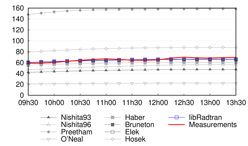
Figure 8: Sky irradiance. The sky irradiance in $W.m^{-2}$ as a function of the time of day (spectral irradiance integrated over the 360-720 $nm$ range).

• the sky irradiance as a function of time, in Fig. 8.

The next sections present the 8 Computer Graphics models we want to evaluate, in chronological order. Each section gives a short overview of the model, some important implementation details if applicable, and then our qualitative and quantitative results.

5 Nishita93 Model

5.1 Overview

The Nishita93 model[1] is one of the first realistic sky rendering algorithms in Computer Graphics. It is based on a numerical integration of the single scattering equation (and thus neglects multiple scattering). For each pixel, an integral along the corresponding view ray is computed numerically. The integrand includes two transmittance terms: one from the viewer to the current sample along the view ray, and one from this sample to the sun. Both terms require a numerical integration. To avoid having to compute a double integral at each pixel, Nishita et al. compute the first term incrementally, while evaluating the outer integral, and precompute the second term in a 2D array.

	Nishita93	Nishita96	Preetham	O’Neal	Haber	Bruneton	Elek	Hosek	libRadtran	Measurements
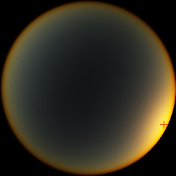
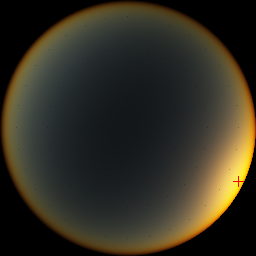
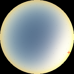
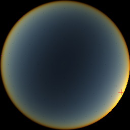
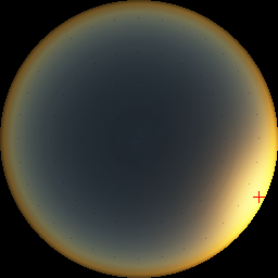
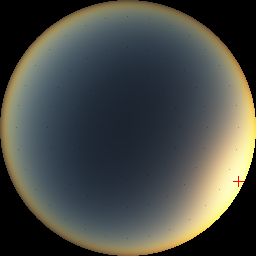
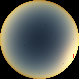
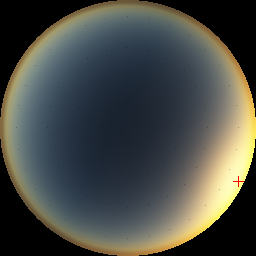
06h00 / 87 °										n/a
10h15 / 41 °
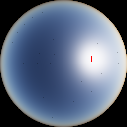
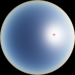
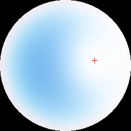
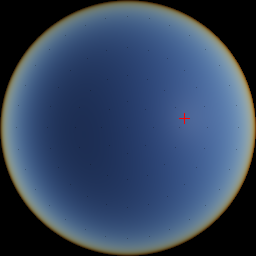
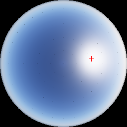
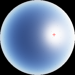
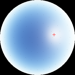
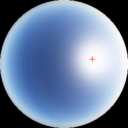
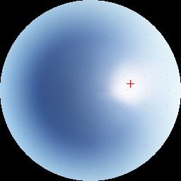
11h15 / 31 °
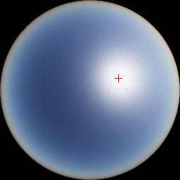
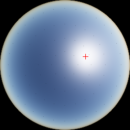
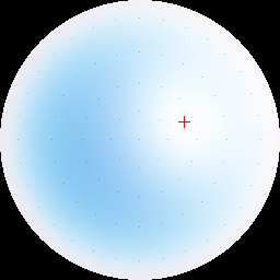
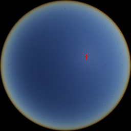
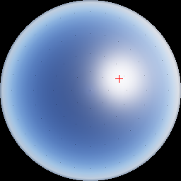
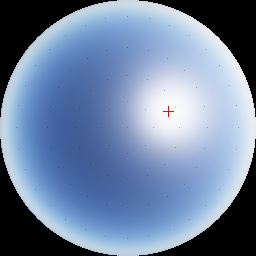
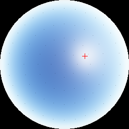
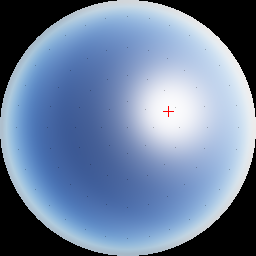
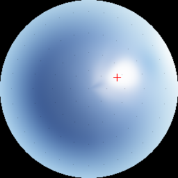
13h15 / 21 °

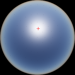
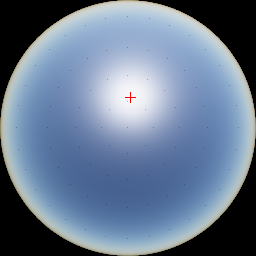
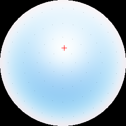
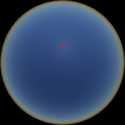
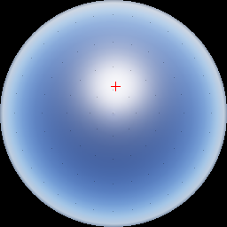
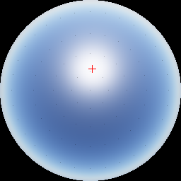
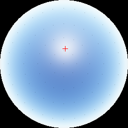
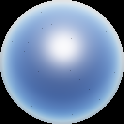
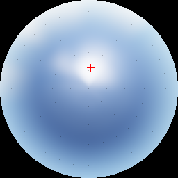
Figure 1: Rendering. Fisheye skydome rendering of the spectral radiance obtained with each model, convolved with the CIE color matching functions, converted from XYZ to linear sRGB, and tone mapped with $1-e^{-kL}$, for several time of day / sun zenith angle values (the red cross indicates the sun direction). The measurements are interpolated using bicubic spherical interpolation before rendering. Compare with Fig. 13 in[9].

5.2 Our Implementation

The Nishita93 model discretizes the atmosphere in concentric layers of constant optical depths (for better precision compared to layers of constant heights), and uses the intersections of these spherical layers with concentric cylinders oriented towards the sun as sampling points for the precomputed 2D array of transmittances. The number of layers and cylinders is not specified in[1]. In our implementation, we use $n_{s}=64$ spheres (i.e. 63 layers) and $n_{c}=64$ cylinders (doubling $n_{s}$ and $n_{c}$ decreases the RMSE by less than 2%).

5.3 Qualitative evaluation

Although this model uses some precomputed data, this data does not depend on the viewer position nor on the sun direction. The model therefore supports all viewpoints from ground to space, aerial perspective (simply by integrating single scattering between the viewer and the terrain), and sun directions below the horizon.

The precomputation phase evaluates a single integral with $O(n_{s})$ samples for all elements of a $n_{s}\times n_{c}$ array, and therefore has $O(n_{s}^{2}n_{c})$ and $O(n_{s}n_{c})$ time and memory complexity, respectively. Thanks to this precomputed table, rendering a pixel has $O(n_{s})$ time complexity (instead of $O(n_{s}^{2})$ without).

5.4 Quantitative evaluation

Our quantitative results, in Figs. 1, 2, 3, 4, 5, 7, 6 and 8, show that this model almost always underestimates the measured values. For instance, computed irradiances (Fig. 8) are about one third less than the measured values. This seems logical since multiple scattering is ignored in this model. This also indicates that, in the measured values, multiple scattering is responsible for one third of the sky irradiance, which seems consistent with[22] (especially the values from Table 1, for a turbidity $T=2$). The RMSE between the Nishita93 model and the measurements, summed over the 17 daytimes, 81 direction samples, and the wavelengths between $360$ and $720\,nm$, is $26.6\ mW/(m^{2}.sr.nm)$.

The relative luminance (Fig. 3) is quite similar to the measurements, but the chromaticity (Fig. 4) shows some differences with the libRadtran results near the horizon and for sunrise and sunset (not measured).

6 Nishita96 Model

6.1 Overview

The Nishita96 model[2] adds (approximate) multiple scattering to the Nishita93 model. The model supports any scattering order, but the authors compute only double scattering. Computing double scattering involves the computation of an integral over all directions, at each sample point along the view ray, with an integrand equal to the single scattering integral. In other words, it requires an additional triple integral at each sample along the view ray. To optimize this computation, Nishita et al. propose to:

• reduce the integral over all directions to a sum over 8 specific directions, called sampling directions, in the plane containing the vertical and sun vectors.

• for each of these 8 directions, precompute the single scattering at the vertices of a $n_{x}\times n_{y}\times n_{z}$ 3D grid having one axis parallel to this direction. Single scattering is computed incrementally, from one vertex to the next along this axis.

Then, at rendering time, 8 trilinearly interpolated lookups into these 8 precomputed tables, at each sample point along the view ray, are sufficient to compute the contribution from double scattering.

	Nishita93	Nishita96	Preetham	O’Neal	Haber	Bruneton	Elek	Hosek	libRadtran	Measurements
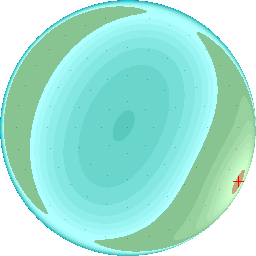
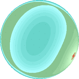
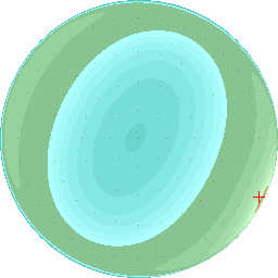
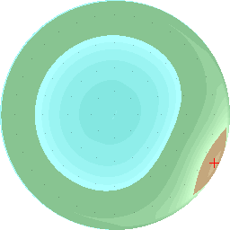
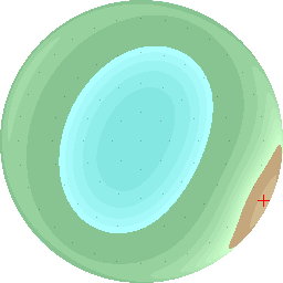
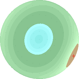
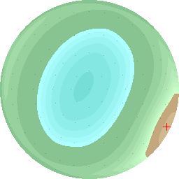
06h00 / 87 °										n/a
10h15 / 41 °
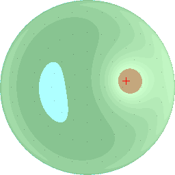
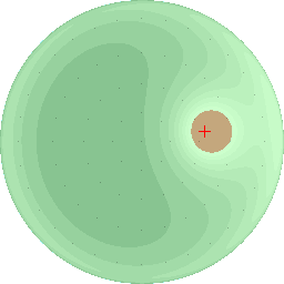
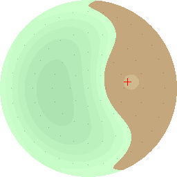
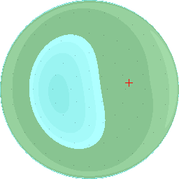
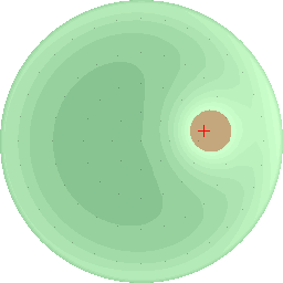
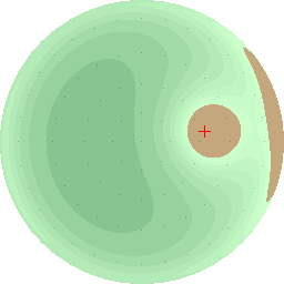
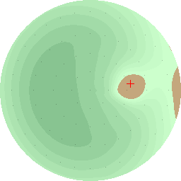
11h15 / 31 °
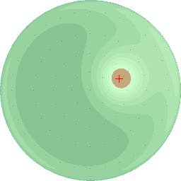
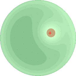
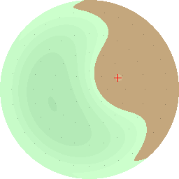
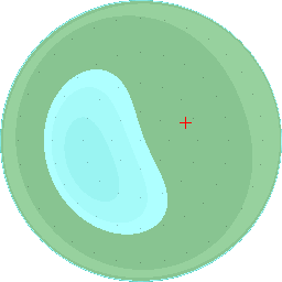
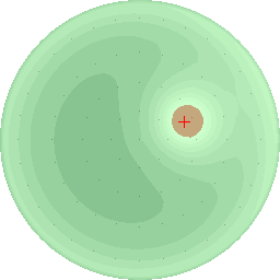
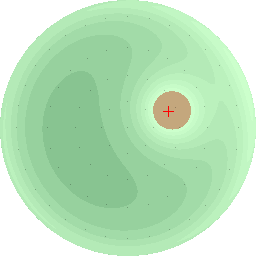
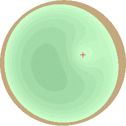
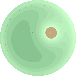
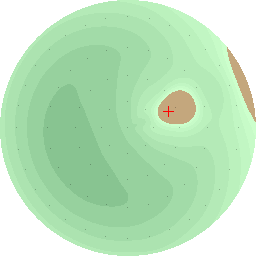
13h15 / 21 °

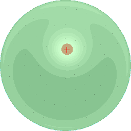
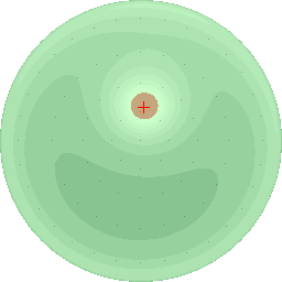
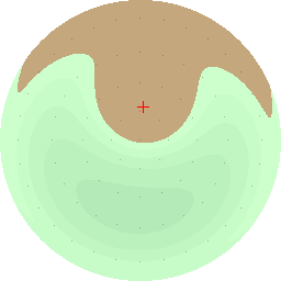
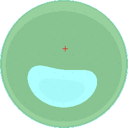
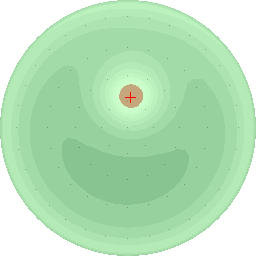
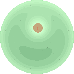
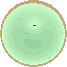
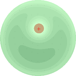
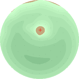
Figure 2: Absolute luminance. The absolute luminance in $cd.m^{-2}$ obtained with each model, using the same color scale as in Fig. 7 in [23]. The measurements are interpolated using bicubic spherical interpolation before being converted to luminance values.

6.2 Our Implementation

In our implementation we use $32^{3}$ voxels for each of the 8 precomputed tables for single scattering. The voxels cover the whole sky dome (i.e. about $1700\times 1700\times 60$ $km$) using 2 orthogonal horizontal axes and a third axis aligned with the sampling direction (or the vertical if the sampling direction is horizontal). We also ignored the third and higher orders of scattering, as in[2], but we did not use Eq. (5) of[2] to compute double scattering. Indeed, this equation seems incorrect to us (one parenthesis is missing, and we couldn’t find a way to get a homogeneous equation by adding it back). Instead, we used the following equation (using the notations from[2] and omitting $\lambda$ parameters):

$$I_{v}=I_{s}\int_{P_{v}}^{P_{a}}e^{-t(s)}\Big{[}R(s,\theta)e^{-t(s^{\prime})}+\int_{4\pi}R(s,\theta_{w})$$

$$\int_{P}^{P_{w}}R(s_{w},\theta^{\prime}_{w})e^{-t(s_{w})-t(s^{\prime}_{w})}\mathrm{d}s_{w}\mathrm{d}w\Big{]}\mathrm{d}s$$

We validated it by comparing its single and double scattering terms with those of the Haber and Bruneton models, which yield similar results (see the supplemental material).

6.3 Qualitative evaluation

The 8 sampling directions are the zenith, the sun direction, the opposites, and the orthogonal, in the same plane, to these four directions. Hence, 4 precomputed tables must be recomputed for each new sun direction. This prevents this model to be used for viewpoints in space, where points with different local sun zenith angles can be viewed simultaneously. On the other hand, aerial perspective and arbitrary sun directions are supported, as in Nishita93.

The algorithmic complexity is dominated by the multiple scattering computations. Assuming we keep 8 sampling directions in all cases, precomputing the single scattering 3D tables has a $O(n_{x}n_{y}n_{z})$ complexity both in time and memory (the time complexity would be $O(n_{x}n_{y}n_{z}^{2})$ without the incremental computation). Rendering a pixel has the same $O(n_{z})$ time complexity as Nishita93, but with a larger constant factor ($n_{z}$ is equivalent to $n_{s}$, and $n_{x}$ and $n_{y}$ to $n_{c}$).

6.4 Quantitative evaluation

Our quantitative results show that the addition of double scattering improves the accuracy of the model, compared to Nishita93. In particular, the RMSE decreases from 26.6  for Nishita93 to 18.3  for Nishita96. However, this model still underestimates the measured values. This is probably due to both the approximate double scattering evaluation (using only 8 directions in a single plane instead of many directions over the whole unit sphere), and the fact that third and higher orders of scattering are not taken into account (since, as we show in the next sections, the models that do not use these approximations are more accurate).

The relative luminance is a bit closer to the measurements, compared to Nishita93, but the chromaticity remains quite different from the libRadtran results near the horizon and for sunrise and sunset (not measured).

7 Preetham Model

7.1 Overview

The Preetham model[3] is an analytical model allowing the computation of the sky color or spectral radiance with a simple mathematical formula. It was obtained by computing sky radiances for many view directions, sun directions, and turbidity values, using the Nishita96 model, and then by fitting the results with an analytical function from Perez et al.[24], using non-linear least square fitting. The resulting model has only one parameter, namely the turbidity. This model is completed with an independent equation for aerial perspective, derived using a flat Earth hypothesis, and with a model for the Sun radiance.

	Nishita93	Nishita96	Preetham	O’Neal	Haber	Bruneton	Elek	Hosek	libRadtran	Measurements
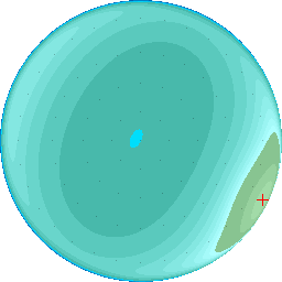
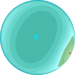
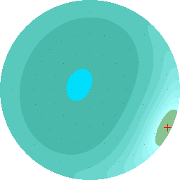
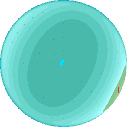
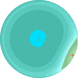
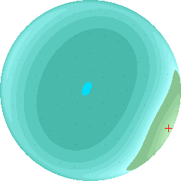
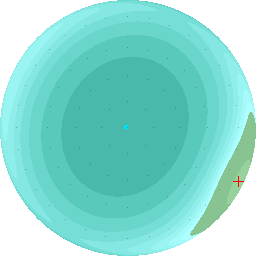
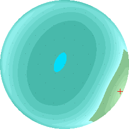
06h00 / 87 °										n/a
10h15 / 41 °
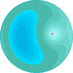
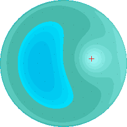
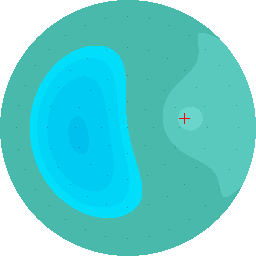
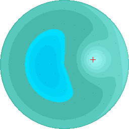
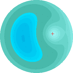
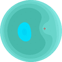
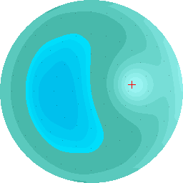
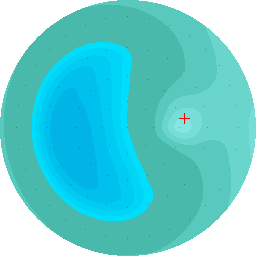
11h15 / 31 °
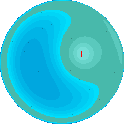
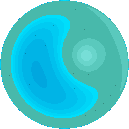
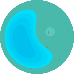
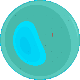
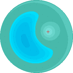
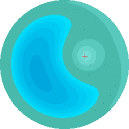
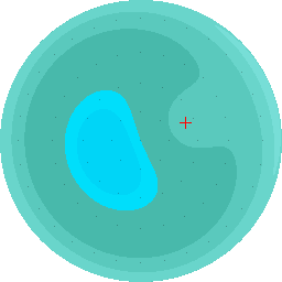
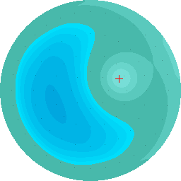
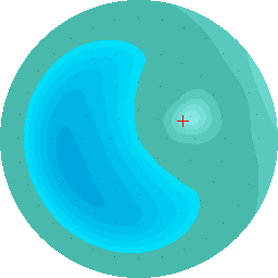
13h15 / 21 °

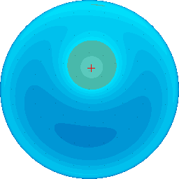
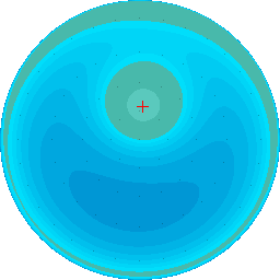
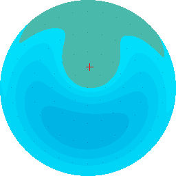
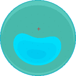
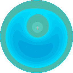
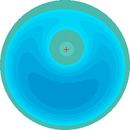
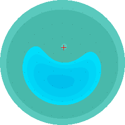
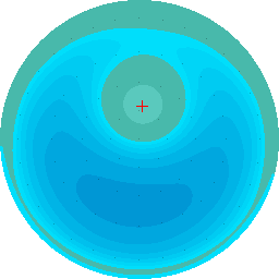
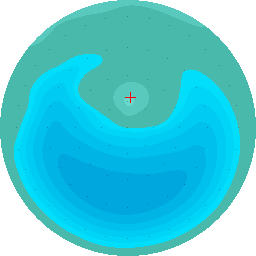
Figure 3: Relative luminance. The luminance obtained with each model, in percentage of the zenith luminance, and using the same color scale as in Fig. 6 in [23]. The measurements are interpolated using bicubic spherical interpolation before being converted to luminance values.

7.2 Our implementation

Our implementation is a straightforward implementation of the equations from[3]. Since the Preetham model has no input parameters for the extraterrestrial solar spectrum, the ground albedo, the phase functions, etc (all already included in the model), we simply ignored these parameters when running the Preetham model.

7.3 Qualitative evaluation

The Preetham model is limited to views from the ground, both because the analytical functions were fitted for an observer at the ground level, and because the separate aerial perspective model assumes a flat Earth hypothesis. It is also limited to sun directions above the horizon. It supports aerial perspective, but with a separate model from the sky model, which could give visual inconsistencies between the two (near the horizon).

The time and memory complexity to render a pixel is simply $O(1)$. There is no precomputation phase at all, if one simply wants to use the model as is. However, if one wants to change some atmospheric parameter, or the ground albedo, it is necessary to recompute the sky radiance for many view directions and sun directions, and perform a new non linear fitting. Using the Nishita96 model, the time and memory complexity of this precomputation would be at least $O(n_{x}n_{y}n_{z}n)$ (for $n$ sun directions).

7.4 Quantitative evaluation

Our quantitative results, which confirm those of Zotti et al. (compare Fig. 2 with Fig. 7 in[23] for $T=2.5$), show that the Preetham model overestimates the measured values, by a large factor (about 2; the RMSE is 88.1 ). The relative luminance and the chromaticity are also quite different from the measured ones and from Nishita96 or libRadtran (especially near the Sun or the horizon).

This is surprising, since this model was fitted using results from the Nishita96 model, which slightly underestimates the measured values. In any case, we believe that the family of analytical functions used by Preetham, fitted directly to the measurements, or to results from libRadtran or another reference model, could produce a much better fit of the measured values (cf the Hosek model in Section 12, which uses very similar analytical functions and gets much better results).

8 O’Neal Model

	Nishita93	Nishita96	Preetham	O’Neal	Haber	Bruneton	Elek	Hosek	libRadtran	Measurements
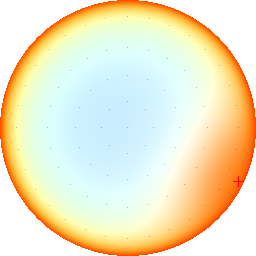
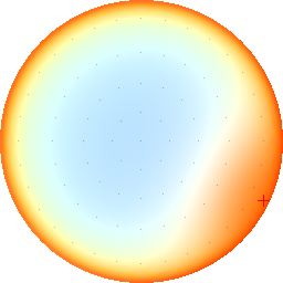
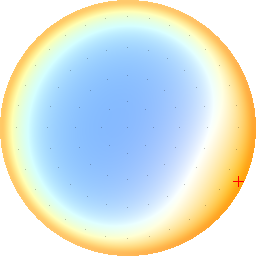
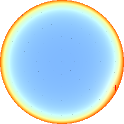
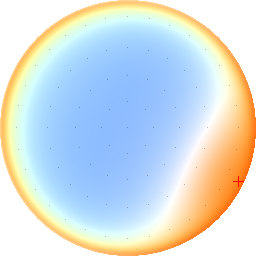
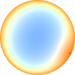
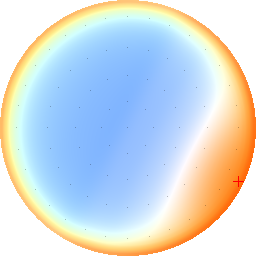
06h00 / 87 °										n/a
10h15 / 41 °
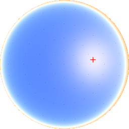
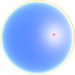
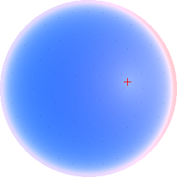
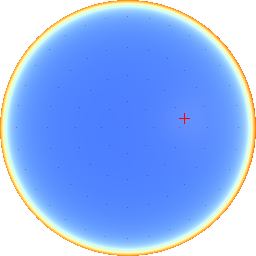
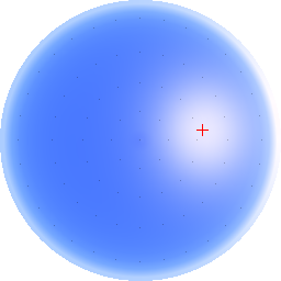
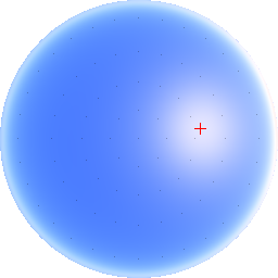
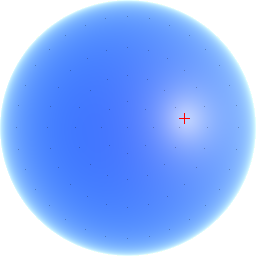
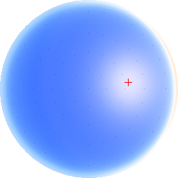
11h15 / 31 °
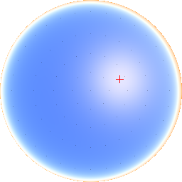
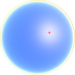
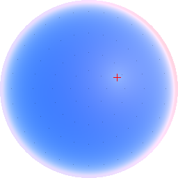
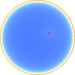
13h15 / 21 °

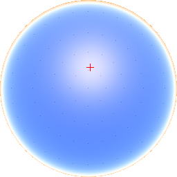
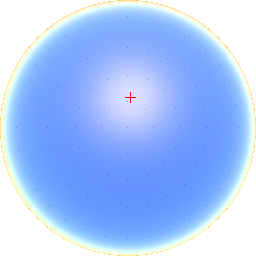
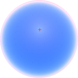
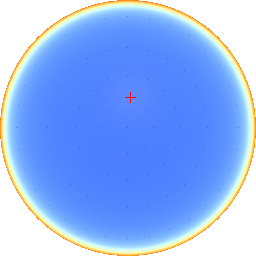
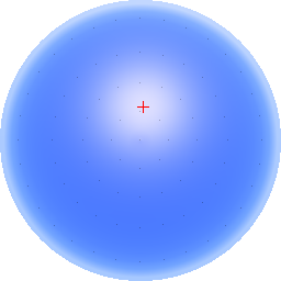
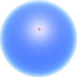
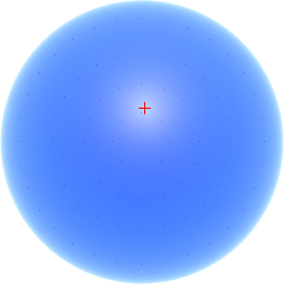
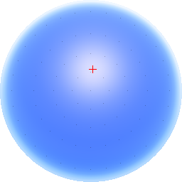
Figure 4: Chromaticity. The rg-chromaticity, $(r,g,b)/\mathrm{max}(r,g,b)$, obtained with each model. The measurements are interpolated using bicubic spherical interpolation before being converted to chromaticity values.

8.1 Overview

The O’Neal model[4] is one of the first atmospheric scattering models running at interactive frame rates on GPU. As in Nishita93, on which it is based, this model uses a numerical integration of the single scattering equation, and neglects multiple scattering. This integration is performed per vertex instead of per pixel, with the phase functions evaluated per pixel to avoid loosing angular precision. The main difference to the Nishita93 model is how transmittance is computed in the numerical integration loop: instead of using a precomputed 2D table (which would require texture fetches from the vertex shader), O’Neal uses an analytic approximation of this 2D function.

8.2 Our Implementation

Our implementation is based on the author’s source code, with some simplifications removed:

• we use two scale height values, one for Rayleigh and one for Mie, as in all the other models (O’Neal uses the same value for both, which divides the number of transmittance terms to evaluate by 2),

• we use the Rayleigh phase function for air molecules (O’Neal lets the user choose between this or an isotropic phase function – cf section 16.5.2 in[4]).

We also replaced the analytic approximation of the transmittance proposed by O’Neal, which is specific to the atmospheric parameters he used, with a generic one based on[25]. Finally, we used 4 samples, instead of 2 in the original source code, to compute each single scattering integral. This is more or less equivalent to using $n_{s}=4$ concentric spheres in Nishita93.

8.3 Qualitative evaluation

The O’Neal model has the same scope as the Nishita93 model, on which it is based. In other words it supports all viewpoints from ground to space, aerial perspective, as well as sun directions below the horizon. Since the precomputed 2D transmittance table is replaced with an analytic approximation there is no precomputation phase, unlike in Nishita93. But this does not change the complexity of the rendering phase, which remains $O(n_{s})$ – although with a smaller constant factor since computations are done per vertex instead of per pixel.

8.4 Quantitative evaluation

Our quantitative results show that the O’Neal model underestimates the measured values, by a large factor (about 3; the RMSE is 49.5 ). The relative luminance and the chromaticity also differ more from the measurements than Nishita93 (especially near the Sun). However, this is mostly due to the number of samples used for the numerical integration. With only 2 samples, as originally proposed by O’Neal, the RMSE is $57.7$. With 32 samples, we get almost the same results as Nishita93 (but this might not be an option for real-time applications, especially on low-end GPUs).

9 Haber Model

	Nishita93	Nishita96	Preetham	O’Neal	Haber	Bruneton	Elek	Hosek	libRadtran
10h15 / 41 °	\begin{overpic}[width=86.72267pt]{relative_error_10h15_nishita93} \put(5.0,5.0){\footnotesize 24.7 } \end{overpic}	\begin{overpic}[width=86.72267pt]{relative_error_10h15_nishita96} \put(5.0,5.0){\footnotesize 17.7 } \end{overpic}	\begin{overpic}[width=86.72267pt]{relative_error_10h15_preetham} \put(5.0,5.0){\footnotesize 92.4 } \end{overpic}	\begin{overpic}[width=86.72267pt]{relative_error_10h15_oneal} \put(5.0,5.0){\footnotesize 49.7 } \end{overpic}	\begin{overpic}[width=86.72267pt]{relative_error_10h15_haber} \put(5.0,5.0){\footnotesize 12.6 } \end{overpic}	\begin{overpic}[width=86.72267pt]{relative_error_10h15_bruneton} \put(5.0,5.0){\footnotesize 9 } \end{overpic}	\begin{overpic}[width=86.72267pt]{relative_error_10h15_elek} \put(5.0,5.0){\footnotesize 9 } \end{overpic}	\begin{overpic}[width=86.72267pt]{relative_error_10h15_hosek} \put(5.0,5.0){\footnotesize 39.9 } \end{overpic}	\begin{overpic}[width=86.72267pt]{relative_error_10h15_libradtran} \put(5.0,5.0){\footnotesize 9.3 } \end{overpic}
11h15 / 31 °	\begin{overpic}[width=86.72267pt]{relative_error_11h15_nishita93} \put(5.0,5.0){\footnotesize 26.8 } \end{overpic}	\begin{overpic}[width=86.72267pt]{relative_error_11h15_nishita96} \put(5.0,5.0){\footnotesize 18.7 } \end{overpic}	\begin{overpic}[width=86.72267pt]{relative_error_11h15_preetham} \put(5.0,5.0){\footnotesize 88.4 } \end{overpic}	\begin{overpic}[width=86.72267pt]{relative_error_11h15_oneal} \put(5.0,5.0){\footnotesize 49.8 } \end{overpic}	\begin{overpic}[width=86.72267pt]{relative_error_11h15_haber} \put(5.0,5.0){\footnotesize 15.2 } \end{overpic}	\begin{overpic}[width=86.72267pt]{relative_error_11h15_bruneton} \put(5.0,5.0){\footnotesize 11.1 } \end{overpic}	\begin{overpic}[width=86.72267pt]{relative_error_11h15_elek} \put(5.0,5.0){\footnotesize 11.1 } \end{overpic}	\begin{overpic}[width=86.72267pt]{relative_error_11h15_hosek} \put(5.0,5.0){\footnotesize 42.8 } \end{overpic}	\begin{overpic}[width=86.72267pt]{relative_error_11h15_libradtran} \put(5.0,5.0){\footnotesize 11.1 } \end{overpic}
13h15 / 21 °	\begin{overpic}[width=86.72267pt]{relative_error_13h15_nishita93} \put(5.0,5.0){\footnotesize 28 } \end{overpic}	\begin{overpic}[width=86.72267pt]{relative_error_13h15_nishita96} \put(5.0,5.0){\footnotesize 17.4 } \end{overpic}	\begin{overpic}[width=86.72267pt]{relative_error_13h15_preetham} \put(5.0,5.0){\footnotesize 83.3 } \end{overpic}	\begin{overpic}[width=86.72267pt]{relative_error_13h15_oneal} \put(5.0,5.0){\footnotesize 48.4 } \end{overpic}	\begin{overpic}[width=86.72267pt]{relative_error_13h15_haber} \put(5.0,5.0){\footnotesize 14.9 } \end{overpic}	\begin{overpic}[width=86.72267pt]{relative_error_13h15_bruneton} \put(5.0,5.0){\footnotesize 11 } \end{overpic}	\begin{overpic}[width=86.72267pt]{relative_error_13h15_elek} \put(5.0,5.0){\footnotesize 11 } \end{overpic}	\begin{overpic}[width=86.72267pt]{relative_error_13h15_hosek} \put(5.0,5.0){\footnotesize 40.5 } \end{overpic}	\begin{overpic}[width=86.72267pt]{relative_error_13h15_libradtran} \put(5.0,5.0){\footnotesize 10.9 } \end{overpic}

Figure 5: Relative error. The relative error compared with the measurements, in % and using the same color scale as in [9], computed at the 81 sampling points (and summed equally over the common range supported by all models, i.e. between $360$ and $720\,nm$), and then interpolated with spherical bicubic interpolation. The bottom left number is the RMSE in $mW/(m^{2}.sr.nm)$ (computed over the 81 sampling points and all the wavelengths between $360$ and $720\,nm$).

9.1 Overview

The Haber model[5] stores the atmospheric properties in $n_{s}$ layers of constant optical depths, as in Nishita93, and uses a 3D grid to compute the successive orders of multiple scattering, as in Nishita96. However, Haber et al. use a $n_{r}\times n_{\theta}\times n_{\phi}$ grid based on spherical coordinates centered on the viewer, instead of the $n_{x}\times n_{y}\times n_{z}$ Cartesian grid used in[2]. Also, they compute multiple scattering more precisely, by integrating over all directions (in fact over all cells) at each grid cell (instead of using only 8 coplanar specific directions as in[2]). The main approximations in their model are:

• the approximation of the Rayleigh phase function with the isotropic phase function, for all scattering orders,

• the approximation of the Mie phase function with a $g$ $\delta$-peak and a $(1-g)$ isotropic lobe, except for single scattering.

The latter approximation reduces to the use of an effective Mie scattering coefficient (see Eq. (2) in[5]), which must also be used in the Mie extinction coefficient to avoid energy losses.

Once the 3D grid is computed, rendering a pixel is done with a numerical integration along the corresponding view ray, with a lookup in the 3D grid per integration sample (plus a computation of the transmittance between the viewer and this sample, which requires a nested integral).

Haber et al. also take into account the refractive index of air, yielding curved light paths, as well as ozone absorption. They also propose algorithmic optimizations for the main loop over all cell pairs – a naive implementation would have a $O(n_{r}^{2}n_{\theta}^{2}n_{\phi}^{2}n_{s})$ complexity.

9.2 Our implementation

In our implementation we neglect the ozone absorption and the refractive index of air. We also ignore the ground albedo, as in[5]. We use $n_{s}=50$ layers and $n_{\phi}=72$ azimuthal directions for the 3D grid (in[5] between 20-50 layers and 72-120 directions are used), yielding a total of 65268 cells, and 4 scattering orders. Finally, we do not use the effective Mie scattering coefficient approximation. Instead, we approximate the Mie phase function with the isotropic phase function and use the raw Mie scattering coefficient (except for single scattering, where we use the Cornette-Shanks phase function, as in[5]). We found this method less error prone (it is hard to make sure the effective scattering coefficient is not used for single scattering, especially in the final pass that combines the single and multiple scattering contributions) and slightly more accurate.

9.3 Qualitative evaluation

The 3D grid of cells used in the Haber model is computed for a specific sun zenith angle, and a specific viewer altitude. Therefore, this model is limited to views on or near the ground (views from space show points with different local sun zenith angles simultaneously). On the other hand, since a pixel is rendered with a numerical integration along the view ray, it is easy to support aerial perspective. Sun directions below the horizon are also supported. In fact, this was the main motivation of this model.

The precomputation phase for the 3D grid, assuming a fixed number of scattering orders, has $O(n_{r}^{2}n_{\theta}^{2}n_{\phi}^{2})$ and $O(n_{r}n_{\theta}n_{\phi})$ time and memory complexity, respectively, thanks to the algorithmic optimizations described in[5]. Rendering a pixel, as described in[5], has a $O(n_{r}n_{s})$ time complexity (because the transmittance is not precomputed, unlike in the previous models), but this can easily be reduced to $O(n_{r})$ with precomputation.

9.4 Quantitative evaluation

Our quantitative results, in particular in Fig. 8, show that the Haber model slightly underestimates the measured values, but less than the Nishita96 model (the RMSE is 14.7 vs 18.3 for Nishita96). This seems logical, since this model takes more scattering orders into account, and uses less approximations to compute each order (but, on the other hand, ignores the ground albedo). Fig. 5 shows that this underestimation is not uniform, and some areas show in fact an overestimation. This is best seen at about 90 degrees from the sun, and is due to the approximation of the Rayleigh phase function with the isotropic phase function (removing this approximation for single scattering only is easy, does not require much more memory, and gives significantly better results).

10 Bruneton Model

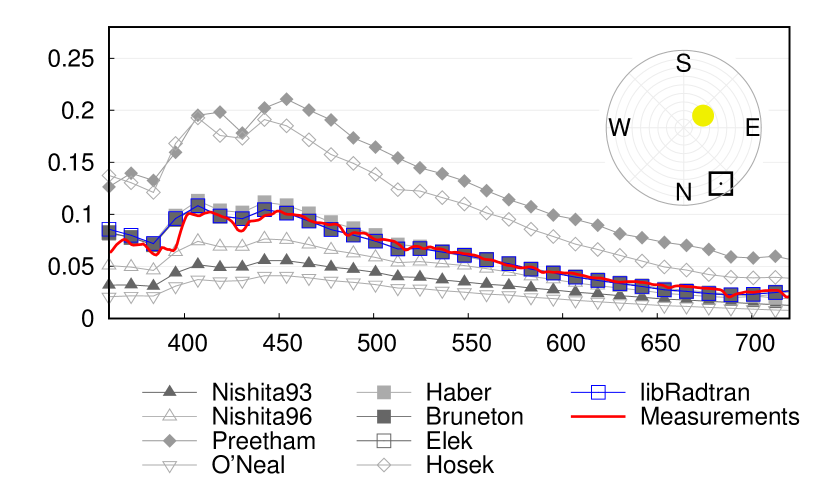
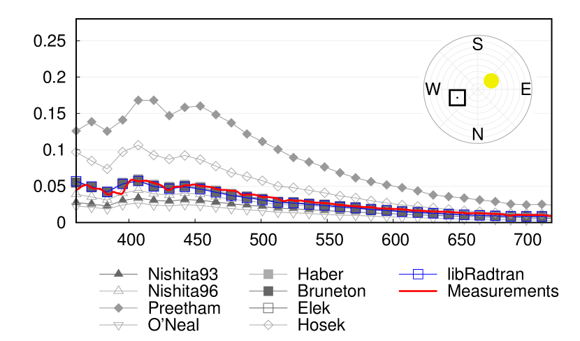
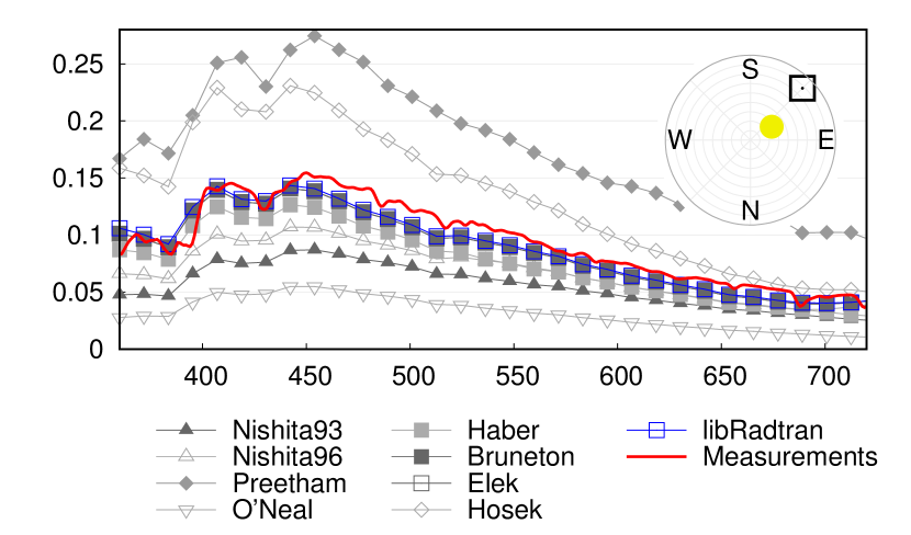
Figure 6: Spectral radiance. Four spectral radiance samples in $W.m^{-2}.sr^{-1}.nm^{-1}$ as a function of wavelength in $nm$, for $t=\mathrm{11h45}$ (sun zenith angle = 27 °). Compare with Fig. 10 in[9].

10.1 Overview

The Bruneton model[6] precomputes the multiple scattering orders in sequence, as in the Nishita96 and Haber models. However, instead of doing this precomputation for a single sun zenith angle, Bruneton et al. do it for $n_{\theta_{s}}$ sun zenith angles, including below the horizon. As a consequence, they need a 4D grid instead of a 3D one as in[2] and[5]. While Nishita96 uses a Cartesian grid, and Haber a grid based on spherical coordinates, the ”grid” used in Bruneton et al. comes from the parameterization used ($n_{r}$ altitudes, $n_{\theta}$ and $n_{\theta_{s}}$ view and sun zenith angles and $n_{\gamma}$ view-sun angles), and has no simple geometric representation. Bruneton et al. take the ground albedo into account (as Nishita96 but unlike Haber), as well as the Rayleigh and Cornette-Shanks phase functions (Haber et al. use some isotropic approximations to save memory and computation time). As in[5], multiple scattering is computed with an integral over all directions at each view ray sample (whereas Nishita96 approximates this using only 8 coplanar directions).

10.2 Our implementation

Our implementation is directly based on the authors source code, simply extended to work with $n_{\lambda}$ (i.e. 40) dimensional vectors instead of RGB values. Because of this, we didn’t use the approximation proposed in Section 4 of[6], which keeps only one spectral value for the single Mie scattering in order to be able to pack the Rayleigh and Mie terms in a single GPU vector. Instead, we store them separately in two 40-dimensional vectors. Finally, we also adapted the code to run on CPU, to make use of the same framework and double precision as in our implementation of the other models. We used the same grid resolution and number of integration samples as in the original code.

10.3 Qualitative evaluation

The Bruneton model supports all viewpoints from ground to space, aerial perspective and sun directions below the horizon.

The most costly precomputation step is the computation of $\Delta J$ in Algorithm 4.1 of[6]. It involves an integral over all directions (of $O(n_{\theta^{\prime}}n_{\phi^{\prime}})$ complexity) for all cells of the 4D $\Delta J$ table, yielding a $O(n_{r}n_{\theta}n_{\theta_{s}}n_{\gamma}n_{\theta^{\prime}}n_{\phi^{\prime}})$ and $O(n_{r}n_{\theta}n_{\theta_{s}}n_{\gamma})$ time and memory complexity, respectively. At render time, the complexity is simply $O(1)$.

10.4 Quantitative evaluation

Our quantitative results show that the Bruneton model gives more accurate results than the Haber model (the RMSE decreases from 14.7 to 11.3 ). The sky radiance is sometimes underestimated (in particular very close to the sun, as all the models), and sometimes overestimated (e.g. near the horizon in the opposite sun direction). However, the Bruneton model gives very close results to the libRadtran reference model, in all quantitative evaluations (see Figs. 1, 2, 3, 4, 5, 7, 6 and 8). This suggests that the difference with the measurements comes from the input parameters used (such as the Mie phase function), and/or from the neglected physical processes (molecular absorption, polarization, etc), rather than from approximations used to solve the physical processes that are taken into account (e.g. insufficient number of samples in some numerical integrals). In particular, the underestimation near the sun, observed in all models including libRadtran, is almost certainly due to a missing strong forward scattering peak in the Cornette-Shanks phase function used to approximate the real Mie phase function.

11 Elek Model

11.1 Overview

The Elek model[7] extends the Bruneton model to arbitrary atmospheres and to oceans. It computes the multiple scattering orders in sequence, as in the Nishita96, Haber and Bruneton models, using mostly the same algorithm, 4D tables and texture parameterizations as in the Bruneton model. However, instead of doing these precomputations on 3 wavelengths, Elek et al. perform them on 15 wavelengths, and convert the results to RGB at the very end of the precomputation phase (leaving the sky rendering phase unchanged).

11.2 Our Implementation

When running all the models with 40 wavelengths, which is what we did for our quantitative evaluations as explained in Section 4.2, the Bruneton and Elek models become identical. For this reason, we used the same implementation for both models.

11.3 Qualitative evaluation

The Elek model supports the same viewpoints as the Bruneton model. It also has the same algorithmic complexity, when both models are run spectrally.

11.4 Quantitative evaluation

Our quantitative results in Figs. 1, 2, 3, 4, 5, 7, 6 and 8 are exactly the same as those of the Bruneton model, since the Elek and Bruneton models are identical when run spectrally. However, when using the original number of wavelengths proposed in each model, the Elek model is more accurate (cf Section 14.3).

12 Hosek Model

12.1 Overview

The Hosek model[8] is an analytical model similar to the Preetham model. The main differences are:

• an improved analytical formula, with a few more degrees of freedom for the fitting phase,

• a fully spectral model (instead of using CIE XYZ values converted at the end to a radiance spectrum), allowing a user specified extraterrestrial solar spectrum,

• new model parameters, in addition to turbidity, for the spectral ground albedo.

Also, the analytical functions were fitted to results obtained with a path-tracer, a priori more accurate than the Nishita96 model used by Preetham.

12.2 Our implementation

Our implementation is a thin wrapper around the authors source code. As with the Preetham model, we set the turbidity to $2.53$. However, unlike with the Preetham model, we also set the extraterrestrial solar spectrum and the spectral ground albedo to the values used in all other models, taking advantage of the fact that the Hosek model handles these parameters.

12.3 Qualitative evaluation

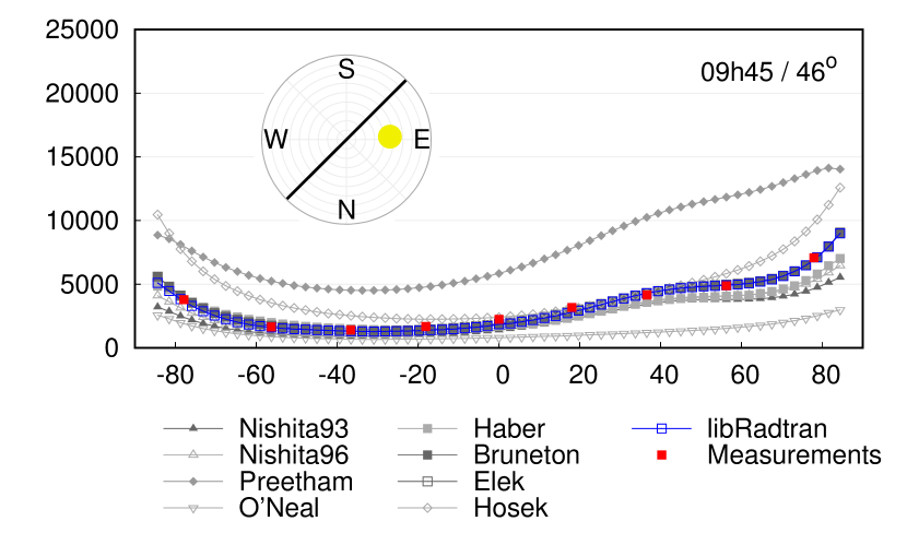
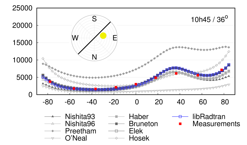
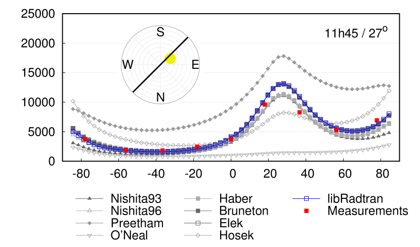
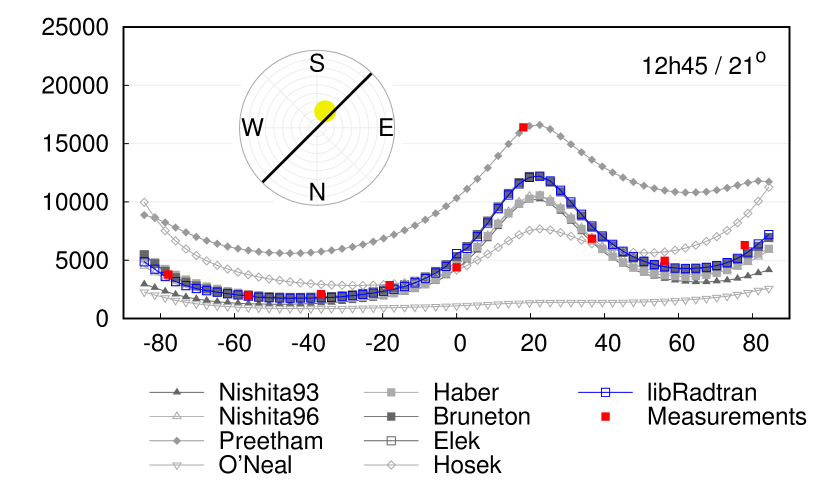
Figure 7: Luminance profiles. The sky luminance in $cd.m^{-2}$ in a fixed vertical plane (black line), as a function the view zenith angle, for different time of day / sun zenith angle values.

The Hosek model is limited to views from the ground, because the analytical functions were fitted for an observer at the ground level. It is also limited to sun directions above the horizon (as explained in[8], supporting these would require different analytic formulae, because the sky radiance pattern is significantly different at sunrise / sunset than during the day). Finally, unlike Preetham, Hosek et al. do not provide a separate model for the aerial perspective, which is thus not supported.

The time and memory complexity to render a pixel is simply $O(1)$. There is no precomputation phase at all, if one simply wants to use the model as is. However, if one wants to change some atmospheric parameter, it is necessary to recompute the sky radiance for many view directions and sun directions, and perform a new non linear fitting.

12.4 Quantitative evaluation

Our quantitative results show that the Hosek model overestimates the measured values, by a large factor (but not as large as for the Preetham model), except near the sun where, on the contrary, it underestimates the measured values. The RMSE is 41.5 .

This is surprising, since this model was fitted using results from a path-tracer using the same physical equations as in all the other models. In any case, we believe that the family of analytical functions used by Hosek et al., fitted directly to the measurements, could produce much better results (in other words, the observed discrepancy is probably not due to the choice of the family of functions used for the fitting).

13 Perceptual study

Nishita93	Nishita96	Preetham	O’Neal	Haber	Bruneton	Elek	Hosek

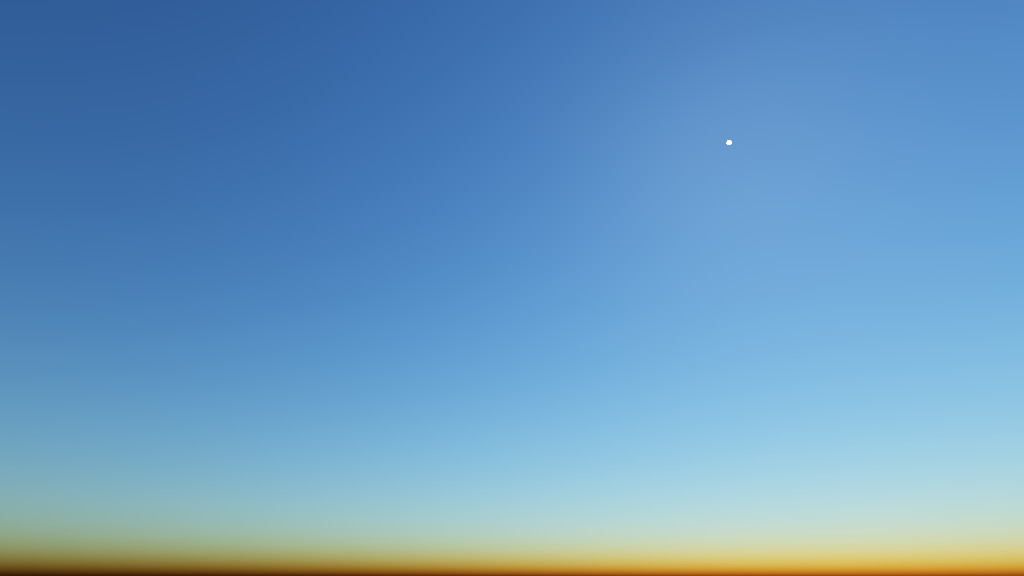
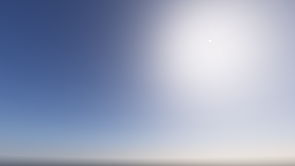
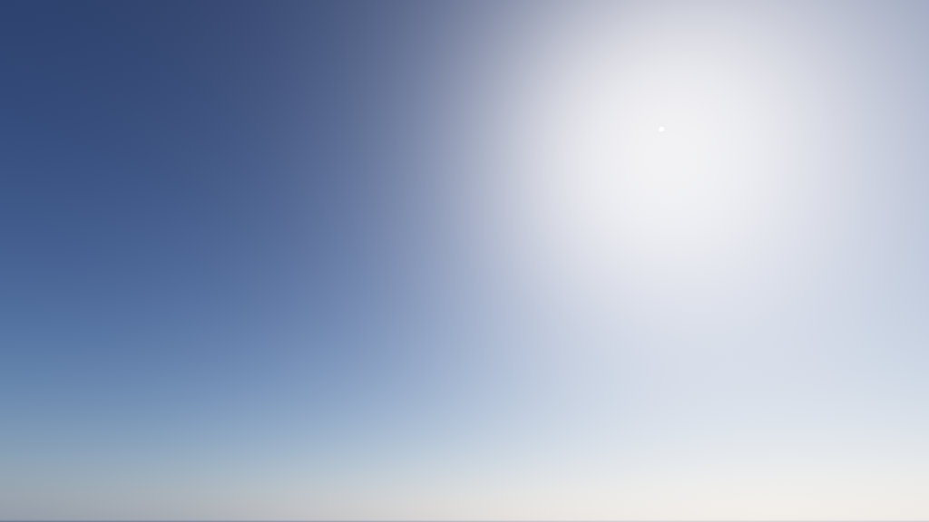
Figure 9: Perceptual study inputs. The images that participants have been asked to compare by pairs (within each row). Since the Nishita93 and Nishita96 images are almost identical, we excluded the Nishita93 model from the study.

While some applications require physical accuracy (e.g. energy studies), other applications only require the sky to look realistic to users. It is thus interesting to evaluate how the models are perceived by users. For this we did a perceptual study, which is presented here.

13.1 Experimental procedure

In order to find which models look the most realistic to users, we asked them to compare pairs of images produced by different models but with identical atmospheric parameters. We asked each participant of the study to compare all the possible pairs, in random order. For each pair, the task was ”Click on the image that you find the most realistic”.

Before running the experiment, we generated the images to compare as follows:

• we chose a viewport including the horizon and the sun (the two areas where the models differ the most), but excluding the ground (not all the models support aerial perspective, which is needed to render the ground in a realistic way),

• we used the same atmospheric parameters as in Section 3 for all the models and we ran each model with the original number of wavelengths proposed by their authors (as described in Section 14.3), in order to evaluate the perceptual impact of this parameter,

• we scaled the results with a uniform per-model factor, before tone-mapping, so that each model gives the same sky irradiance (indeed, we are not interested in absolute values here).

The resulting images are shown in Fig. 9 (we used two scenes: a sunrise and a morning sky). Since the images for Nishita93 and Nishita96 are almost identical, we decided to exclude the Nishita93 model from the experiment.

Our experiment was conducted with 25 participants in a dark room, on a calibrated HP ZR2440w monitor (24-inch, gamma $2.2$, color temperature $6500\,K$, viewing distance $70\,\mathrm{cm}$). We also did the same experiment online with 105 participants provided by Prolific.ac (using their desktop computer in an uncontrolled environment – see the supplemental material).

13.2 Analysis methodology

The result of the study is a preference matrix $A$ where $A_{i,j}$ is the number of participants who find the model in row $i$ more realistic than the model in column $j$. From this we can compute a score $a_{i}=\sum_{j\neq i}A_{i,j}$ for each model, which we can use to rank the models. However, not all score differences are statistically significant. We consider that there is a statistically significant difference between the realism of two models if their score difference is larger than the value $\lceil R_{c}\rceil$ defined in [26] (following the same methodology as [26, 27]).

TABLE I: Perceptual study results. The preference matrix, the model scores (total number of votes, in bold) and the model groups, for the sunrise (top) and morning (bottom) sky perceptual studies. $M_{1},\ldots,M_{7}$ correspond respectively to the Nishita96, Preetham, O’Neal, Haber, Bruneton, Elek and Hosek models.

	$M_{1}$	$M_{2}$	$M_{3}$	$M_{4}$	$M_{5}$	$M_{6}$	$M_{7}$	Total
$M_{1}$	-	18	12	3	13	9	11	66
$M_{2}$	7	-	12	1	4	3	4	31
$M_{3}$	13	13	-	6	7	10	11	60
$M_{4}$	22	24	19	-	20	17	20	122
$M_{5}$	12	21	18	5	-	14	18	88
$M_{6}$	16	22	15	8	11	-	14	86
$M_{7}$	14	21	14	5	7	11	-	72

  $M_{2}$   

  $M_{3}$   

  $M_{1}$            

  $M_{7}$            

  $M_{6}$            

  $M_{5}$   

  $M_{4}$   

($\lceil R_{c}\rceil=28$)

	$M_{1}$	$M_{2}$	$M_{3}$	$M_{4}$	$M_{5}$	$M_{6}$	$M_{7}$	Total
$M_{1}$	-	18	19	14	10	13	6	80
$M_{2}$	7	-	14	6	4	5	5	41
$M_{3}$	6	11	-	8	4	11	7	47
$M_{4}$	11	19	17	-	8	13	10	78
$M_{5}$	15	21	21	17	-	18	13	105
$M_{6}$	12	20	14	12	7	-	5	70
$M_{7}$	19	20	18	15	12	20	-	104

  $M_{2}$   

  $M_{3}$            

  $M_{6}$            

  $M_{4}$            

  $M_{1}$            

  $M_{7}$   

  $M_{5}$   

($\lceil R_{c}\rceil=28$)

13.3 Experiment results

TABLE II: Qualitative comparison. Summary of the qualitive evaluation of the 8 clear sky models. The precomputation time and memory complexity for the Haber and Nishita96 models is for a single Sun zenith angle $\theta_{s}$ only – the Bruneton and Elek models precomputations are for $n$ such angles and the Nishita93 precomputations are independent of $\theta_{s}$.

	Supported	Aerial	Sunset	Scattering	Precompute	Precompute	Render	RMSE
Model	viewpoints	perspective	sunrise	orders	time	memory	time	$mW/(m^{2}.sr.nm)$
Nishita93	all	yes	yes	1	$O(n^{3})$	$O(n^{2})$	$O(n)$

Nishita96 in atmosphere yes yes 2 $O(n^{3})$ $O(n^{3})$ $O(n)$ 18.3 Preetham ground only yes no 2 $0$ $0$ $O(1)$ 88.1 O’Neal all yes yes $1$ $0$ $0$ $O(n)$ 49.5 Haber ground only yes yes all $O(n^{6})$ $O(n^{3})$ $O(n^{2})$ 14.7 Bruneton all yes yes all $O(n^{6})$ $O(n^{4})$ $O(1)$ 11.3 Elek all yes yes all $O(n^{6})$ $O(n^{4})$ $O(1)$ 11.3 Hosek ground only no no all $0$ $0$ $O(1)$ 41.5

The preference matrix and model scores of each scene are shown in Table I, together with the statistically significant score difference $\lceil R_{c}\rceil$, for the significance level $\alpha=0.05$. Grouping together the models whose score difference is less than this threshold gives the groups shown in Table I.

For the sunrise scene the participants find the Haber model significantly more realistic than the Bruneton, Elek, Hosek and Nishita96 models (between which there is no statistically significant differences), while the Preetham and O’Neal models are perceived as the less realistic.

For the morning scene the participants find the Bruneton, Hosek, Nishita96 and Haber models more realistic (with no statistically significant differences between them), followed by the Elek model, with the Preetham and O’Neal models perceived again as the less realistic.

The online experiment gives almost the same ranking as the laboratory experiment for the morning scene, but gives more different results for the sunrise scene (Preetham and O’Neal are still perceived as ones of the less realistic models, but the Haber model is no longer perceived as significantly more realistic than the Bruneton, Elek and Hosek models – see the supplemental material). This suggests that the viewing conditions play an important role in the perceived realism of sunrise and sunset scenes.

Overall, these results show that the less physically accurate models, according to our results in Section 13.3, i.e. the Preetham and O’Neal models, are also perceived as less realistic by the participants. Conversely, the more physically accurate models are perceived as more realistic. However, it seems that participants perceive models whose physical accuracy is ”good enough” as equally realistic.

14 Discussion

This section compares our results with previous work, summarizes the advantages and drawbacks of the models presented above, and discusses some possible ways to improve the accuracy of clear sky models in Computer Graphics.

14.1 Comparison with previous work

According to our results, the clear sky models, sorted in increasing order of physical accuracy in $W/(m^{2}.sr.nm)$, are Preetham, O’Neal, Hosek, Nishita93, Nishita96, Haber, Bruneton and Elek (cf Section 13.3). We also get a very similar order when measured after RGB conversion and tone mapping (cf Fig. 10). According to Kider et al., the most accurate models are Nishita93 and Nishita96 (cf Figs 1, 12 and 15 in[9]). This is problematic, since both papers aim at comparing the models with each other and with a ground thruth. We believe our results are more plausible because:

• the order we get corresponds to a decreasing order of approximations: from the models which approximate all the parameters with a single one, to the models with more parameters and less and less approximations for multiple scattering. In other words, we find that the less approximations are made the more accurate is the result, which seems natural,

• we get the same results for Preetham as in[23] (compare Fig. 3 and Fig. 2 with Figs. 6 and 7 in[23]),

• we get similar results for the single and double scattering components of the Nishita96, Haber and Bruneton models, although the 3 implementations are completely different (see the supplemental material),

• we get almost identical results for the Bruneton and Elek models as libRadtran.

14.2 Advantages and drawbacks

The analytical models, i.e. the Preetham and Hosek models, are fast, memory efficient, easy to implement and don’t require a precomputation phase (see Section 13.3). On the other hand, they are limited to ground level views and require a separate model for aerial perspective (which is not always provided). They also have very few parameters, which limits the range of atmospheric conditions they can reproduce. Our results confirm the results from[23, 9], i.e. that the Hosek model is more accurate than the Preetham model.

Conversely, the numerical models, i.e. the Nishita, O’Neal, Haber, Bruneton and Elek models, are slower, use more memory, are more complex and generally require a precomputation phase, but they can support more viewpoints, include aerial perspective, and provide more physical parameters (and can thus better fit real data).

Amongst the numerical models, the Nishita93 and O’Neal models are the simplest and the ones which require the less memory. Their main drawback is that they ignore multiple scattering, which limits their accuracy, especially for sunrise and sunset. The Nishita96 model adds support for multiple scattering, with some coarse approximations. This increases its accuracy, at the price of increased complexity, rendering times and memory needs. Another drawback is that the precomputation phase must be re-executed each time the Sun zenith angle changes. The Haber model also supports multiple scattering, with less approximations than in the Nishita96 model. This increases its accuracy compared to Nishita96, at the price of longer precomputations and less supported viewpoints. Its main drawbacks are that the precomputation phase must be re-executed each time the Sun zenith angle changes (as in Nishita96) and the approximation of the Rayleigh phase function with the isotropic phase function, which limits its accuracy. The Bruneton model does not use this approximation to compute multiple scattering, and precomputes data for all Sun zenith angles. This increases its accuracy compared to the Haber model, at the price of increased memory needs. The Elek model uses more wavelengths, which increases its accuracy compared to the Bruneton model (cf the next section), at the cost of a longer precomputation phase.

	Nishita93	Nishita96	Preetham	O’Neal	Haber	Bruneton	Elek	Hosek	libRadtran	Measurements
original	\begin{overpic}[width=85.85591pt]{image_original_10h15_nishita93} \put(5.0,5.0){\footnotesize\color[rgb]{1,1,1}45.4 } \put(82.0,85.0){\footnotesize\color[rgb]{1,1,1}\hskip 3.98337pt3} \end{overpic}	\begin{overpic}[width=85.85591pt]{image_original_10h15_nishita96} \put(5.0,5.0){\footnotesize\color[rgb]{1,1,1}29.4 } \put(82.0,85.0){\footnotesize\color[rgb]{1,1,1}\hskip 3.98337pt3} \end{overpic}	\begin{overpic}[width=85.85591pt]{image_original_10h15_preetham} \put(5.0,5.0){\footnotesize\color[rgb]{1,1,1}74.9 } \put(82.0,85.0){\footnotesize\color[rgb]{1,1,1}\hskip 3.98337pt3} \end{overpic}	\begin{overpic}[width=85.85591pt]{image_original_10h15_oneal} \put(5.0,5.0){\footnotesize\color[rgb]{1,1,1}100.6 } \put(82.0,85.0){\footnotesize\color[rgb]{1,1,1}\hskip 3.98337pt3} \end{overpic}	\begin{overpic}[width=85.85591pt]{image_original_10h15_haber} \put(5.0,5.0){\footnotesize\color[rgb]{1,1,1}16.1 } \put(82.0,85.0){\footnotesize\color[rgb]{1,1,1}\hskip 3.98337pt8} \end{overpic}	\begin{overpic}[width=85.85591pt]{image_original_10h15_bruneton} \put(5.0,5.0){\footnotesize\color[rgb]{1,1,1}16 } \put(82.0,85.0){\footnotesize\color[rgb]{1,1,1}\hskip 3.98337pt3} \end{overpic}	\begin{overpic}[width=85.85591pt]{image_original_10h15_elek} \put(5.0,5.0){\footnotesize\color[rgb]{1,1,1}8.8 } \put(82.0,85.0){\footnotesize\color[rgb]{1,1,1}15} \end{overpic}	\begin{overpic}[width=85.85591pt]{image_original_10h15_hosek} \put(5.0,5.0){\footnotesize\color[rgb]{1,1,1}44.8 } \put(82.0,85.0){\footnotesize\color[rgb]{1,1,1}11} \end{overpic}	\begin{overpic}[width=85.85591pt]{image_original_10h15_libradtran} \put(5.0,5.0){\footnotesize\color[rgb]{1,1,1}10.1 } \put(82.0,85.0){\footnotesize\color[rgb]{1,1,1}40} \end{overpic}	\begin{overpic}[width=85.85591pt]{image_original_10h15_measurements} \put(82.0,85.0){\footnotesize\color[rgb]{1,1,1}40} \end{overpic}
Eq. 1	\begin{overpic}[width=85.85591pt]{image_full_spectral_10h15_nishita93} \put(5.0,5.0){\footnotesize\color[rgb]{1,1,1}42.9 } \end{overpic}	\begin{overpic}[width=85.85591pt]{image_full_spectral_10h15_nishita96} \put(5.0,5.0){\footnotesize\color[rgb]{1,1,1}25.6 } \end{overpic}	\begin{overpic}[width=85.85591pt]{image_full_spectral_10h15_preetham} \put(5.0,5.0){\footnotesize\color[rgb]{1,1,1}78 } \end{overpic}	\begin{overpic}[width=85.85591pt]{image_full_spectral_10h15_oneal} \put(5.0,5.0){\footnotesize\color[rgb]{1,1,1}97.3 } \end{overpic}	\begin{overpic}[width=85.85591pt]{image_full_spectral_10h15_haber} \put(5.0,5.0){\footnotesize\color[rgb]{1,1,1}16 } \end{overpic}	\begin{overpic}[width=85.85591pt]{image_full_spectral_10h15_bruneton} \put(5.0,5.0){\footnotesize\color[rgb]{1,1,1}8.8 } \end{overpic}	\begin{overpic}[width=85.85591pt]{image_full_spectral_10h15_elek} \put(5.0,5.0){\footnotesize\color[rgb]{1,1,1}8.8 } \end{overpic}	\begin{overpic}[width=85.85591pt]{image_full_spectral_10h15_hosek} \put(5.0,5.0){\footnotesize\color[rgb]{1,1,1}45.3 } \end{overpic}	\begin{overpic}[width=85.85591pt]{image_full_spectral_10h15_libradtran} \put(5.0,5.0){\footnotesize\color[rgb]{1,1,1}10.1 } \end{overpic}	\begin{overpic}[width=85.85591pt]{image_full_spectral_10h15_measurements} \end{overpic}
Eq. 2	\begin{overpic}[width=85.85591pt]{image_approx_spectral_10h15_nishita93} \put(5.0,5.0){\footnotesize\color[rgb]{1,1,1}43.1 } \end{overpic}	\begin{overpic}[width=85.85591pt]{image_approx_spectral_10h15_nishita96} \put(5.0,5.0){\footnotesize\color[rgb]{1,1,1}25.6 } \end{overpic}	\begin{overpic}[width=85.85591pt]{image_approx_spectral_10h15_preetham} \put(5.0,5.0){\footnotesize\color[rgb]{1,1,1}80.9 } \end{overpic}	\begin{overpic}[width=85.85591pt]{image_approx_spectral_10h15_oneal} \put(5.0,5.0){\footnotesize\color[rgb]{1,1,1}98.2 } \end{overpic}	\begin{overpic}[width=85.85591pt]{image_approx_spectral_10h15_haber} \put(5.0,5.0){\footnotesize\color[rgb]{1,1,1}15.4 } \end{overpic}	\begin{overpic}[width=85.85591pt]{image_approx_spectral_10h15_bruneton} \put(5.0,5.0){\footnotesize\color[rgb]{1,1,1}9.5 } \end{overpic}	\begin{overpic}[width=85.85591pt]{image_approx_spectral_10h15_elek} \put(5.0,5.0){\footnotesize\color[rgb]{1,1,1}9.5 } \end{overpic}	\begin{overpic}[width=85.85591pt]{image_approx_spectral_10h15_hosek} \put(5.0,5.0){\footnotesize\color[rgb]{1,1,1}44.6 } \end{overpic}	\begin{overpic}[width=85.85591pt]{image_approx_spectral_10h15_libradtran} \put(5.0,5.0){\footnotesize\color[rgb]{1,1,1}11.2 } \end{overpic}	\begin{overpic}[width=85.85591pt]{image_approx_spectral_10h15_measurements} \end{overpic}
$10|\mathrm{(1)}-\mathrm{(2)}|$	\begin{overpic}[width=85.85591pt]{image_approx_diff_10h15_nishita93} \put(5.0,5.0){\footnotesize\color[rgb]{1,1,1}41.2 dB} \end{overpic}	\begin{overpic}[width=85.85591pt]{image_approx_diff_10h15_nishita96} \put(5.0,5.0){\footnotesize\color[rgb]{1,1,1}41.7 dB} \end{overpic}	\begin{overpic}[width=85.85591pt]{image_approx_diff_10h15_preetham} \put(5.0,5.0){\footnotesize\color[rgb]{1,1,1}38.3 dB} \end{overpic}	\begin{overpic}[width=85.85591pt]{image_approx_diff_10h15_oneal} \put(5.0,5.0){\footnotesize\color[rgb]{1,1,1}42.9 dB} \end{overpic}	\begin{overpic}[width=85.85591pt]{image_approx_diff_10h15_haber} \put(5.0,5.0){\footnotesize\color[rgb]{1,1,1}42 dB} \end{overpic}	\begin{overpic}[width=85.85591pt]{image_approx_diff_10h15_bruneton} \put(5.0,5.0){\footnotesize\color[rgb]{1,1,1}42.3 dB} \end{overpic}	\begin{overpic}[width=85.85591pt]{image_approx_diff_10h15_elek} \put(5.0,5.0){\footnotesize\color[rgb]{1,1,1}42.3 dB} \end{overpic}	\begin{overpic}[width=85.85591pt]{image_approx_diff_10h15_hosek} \put(5.0,5.0){\footnotesize\color[rgb]{1,1,1}44.1 dB} \end{overpic}	\begin{overpic}[width=85.85591pt]{image_approx_diff_10h15_libradtran} \put(5.0,5.0){\footnotesize\color[rgb]{1,1,1}41.8 dB} \end{overpic}	\begin{overpic}[width=85.85591pt]{image_approx_diff_10h15_measurements} \put(5.0,5.0){\footnotesize\color[rgb]{1,1,1}39.3 dB} \end{overpic}

Figure 10: Spectrum sampling. Rendering of the skydome by using the number of wavelengths $n_{\lambda}$ proposed by the authors of each model (1st row, $n_{\lambda}$ in the top right), by using $n_{\lambda}=40$ and Eq. 1 (2nd row), and by using $n_{\lambda}=3$ and Eq. 2 (3rd row). The bottom left number in each cell is the RMSE, times 1000, compared to the top right cell (summed over the 81 measurement samples, on the RGB colors tone-mapped to the $[0,1]$ interval). The 4th row is the difference between the 2nd and 3rd ones, times 10, with the corresponding peak signal to noise ratio (PSNR).

Finally, an important conclusion from the above comparisons is that none of the models is ”perfectly” accurate, and that there is still room for improvement in this area (although users do not necessarily prefer the most accurate models – cf Section 13). Some ideas to increase accuracy include using more wavelengths, taking polarization into account, or modeling aerosol optical properties more precisely. In the next sections we show that only the latter could potentially significantly increase accuracy.

14.3 Spectrum sampling

In sections 5 to 12 we evaluated the models by using 40 wavelengths between $360\,nm$ and $830\,nm$ as in[9], although the models originally use between 3 and 15 wavelengths. Here we discuss the impact of the number of wavelength samples used on the accuracy of the results. We show that it is possible to use only 3 samples to reconstruct RGB colors or full spectrums, with almost the same accuracy as with 40 samples.

RGB rendering

In order to evaluate the impact of the number of wavelengths $n_{\lambda}$ used to compute the final RGB color, we ran each model with the original number of wavelengths proposed by their authors (or 3 if not specified). Also, for the special case $n_{\lambda}=3$, we used the 3 spectral radiance samples directly as RGB components, instead of converting them to RGB via the CIE color matching functions (which, as pointed out in[7], is incorrect – but is done in the authors implementation of the O’Neal and Bruneton models).

The results do not show significant differences between $n_{\lambda}=40,\ 15,\ 11\ \mathrm{or}\ 8$ (see Fig. 10 and the supplemental material). However, they clearly show that using a constant solar spectrum and 3 spectral radiance samples directly as RGB components significantly decreases the accuracy. In the following we propose a sound and more accurate method to convert these 3 samples to an RGB color.

With the reference spectral method the linear sRGB components are given by

$$[c_{r},c_{g},c_{b}]=\int_{\lambda_{\mathrm{min}}}^{\lambda_{\mathrm{max}}}[\tilde{r}(\lambda),\tilde{g}(\lambda),\tilde{b}(\lambda)]L(\lambda)\mathrm{d}\lambda$$ (1)

where $[\tilde{r},\tilde{g},\tilde{b}]^{\top}=M[\bar{x},\bar{y},\bar{z}]^{\top}$ are color matching functions computed from the XYZ color matching functions $\bar{x},\bar{y},\bar{z}$ and from the XYZ to linear sRGB conversion matrix $M$. Using our knowledge that the sky spectral radiance $L(\lambda)$ is proportional to the extraterrestrial solar spectrum $S(\lambda)$ and to $\lambda^{-4}$ without aerosols, we can approximate $L(\lambda)$ near some $\lambda_{0}$ with $L(\lambda_{0})S(\lambda)\lambda^{-\alpha}/S(\lambda_{0}){\lambda_{0}}^{-\alpha}$, where $\alpha\leq 4$ due to aerosols. Substituting this in Eq. 1 for 3 wavelengths $\lambda_{r},\lambda_{g},\lambda_{b}$ we get

$$[c_{r},c_{g},c_{b}]\approx[k_{r}L(\lambda_{r}),k_{g}L(\lambda_{g}),k_{b}L(\lambda_{b})]$$ (2)

where $k_{r}=\int_{\lambda_{\mathrm{min}}}^{\lambda_{\mathrm{max}}}\tilde{r}(\lambda)\left(S(\lambda)\lambda^{-\alpha}/S(\lambda_{r}){\lambda_{r}}^{-\alpha}\right)\mathrm{d}\lambda$, and similarly for $k_{g}$ and $k_{b}$ (in our results we used $\alpha=3$ and $\lambda_{r},\lambda_{g},\lambda_{b}=680,550,440\,nm$). In other words, we can compute an RGB color by multiplying 3 spectrum samples $L(\lambda_{r}),L(\lambda_{g}),L(\lambda_{b})$ by 3 constants. And, as shown in Fig. 10, this approximation is almost as accurate as with 40 wavelengths (the PSNR is about $40\,\mathrm{dB}$, for all models).

Spectral rendering

For applications that require the sky spectral radiance $L(\lambda)$ at $n_{\lambda}$ wavelengths (e.g. energy studies), we can either compute $L$ for each wavelength, or we can compute $L$ for a smaller number of wavelengths, and extrapolate its value for the other wavelengths, to save computations. We show here that we can reconstruct a full spectrum from only 3 samples with a very small approximation error.

A simple method to reconstruct $L(\lambda)$ from 3 samples $L(\lambda_{r}),L(\lambda_{g}),L(\lambda_{b})$ is to express it as a linear combination of the 3 CIE D65 standard illuminant components [28], as in [3]. This approximation is quite accurate, but we found that the following method, slightly less simple, is much more accurate:

• convert $L(\lambda_{r}),L(\lambda_{g}),L(\lambda_{b})$ to sRGB using Eq. 2,

• convert from sRGB to XYZ and then to xyY,

• convert the xyY color to a full spectrum as in [3].

Our results, in Section 14.3, show that this approximation increases the RMSE by less than $1\,mW/(m^{2}.sr.nm)$, compared to a full computation with 40 wavelengths.

TABLE III: Spectrum sampling. The RMSE in $mW/(m^{2}.sr.nm)$, summed over the 17 daytimes, 81 directions, and $\lambda$ from $360$ to $720\,nm$. Left: spectral radiance computed separately for each wavelength. Right: approximate spectrum reconstructed from 3 spectral radiance computations.

& 26.4 Nishita96 18.3 19.2 Preetham 88.1 88.9 O’Neal 49.5 49.5 Haber 14.7 14.4 Bruneton 11.3 11.4 Elek 11.3 11.4 Hosek 41.5 39

14.4 Polarization

Another idea to increase accuracy is to take polarization into account. Although the Sun light is initially not polarized, it becomes (partially) linearly polarized after the first scattering event in the atmosphere. Because of this, after two scattering events at $90^{\circ}$, the scattered intensity can be null, a phenomenon that can’t be simulated if polarization is ignored. Can we then significantly increase the accuracy of the Computer Graphics clear sky models by taking polarization into account?

To answer this we used the polradtran solver in libRadtran, which can take polarization into account or not, and we compared the results obtained with or without polarization, for the same atmosphere model (due to some polradtran restrictions we couldn’t use the atmosphere properties from Section 3.4. Instead, we used default atmosphere and aerosols properties provided with libRadtran). Our results, in Fig. 11, show that the difference between the two is very small, much smaller than the difference between the CG models and the measurements. In other words, taking polarization into account would not significantly increase their accuracy.

14.5 Aerosol properties

The Computer Graphics clear sky models use very few parameters for the aerosols. The analytical models use only one parameter, the turbidity, while the others generally use the aerosols scattering and absorption coefficients, their scale height, and the asymmetry factor $g$ of their phase function. In contrast, libRadtran can use any number of layers, where each layer can specify wavelength-dependent parameters and arbitrary phase functions. We think adding more aerosol parameters in the CG models is the best way to significantly increase their accuracy. Also, unlike adding more wavelengths or supporting polarization, this would not significantly decrease their performance.

In particular, we think using more realistic phase functions for aerosols is the easiest way to increase accuracy in the solar aureole region. Indeed, all the CG models are quite inaccurate in this region, where single scattering due to aerosols is the most significant term. And, comparing the Cornette-Shanks[19] phase function with a typical aerosol phase function clearly shows that the analytical model is not really accurate for scattering angles smaller than 20 degrees (see Fig. 12).

\begin{overpic}[width=108.405pt]{absolute_luminance_sza30_polradtran_vector} \end{overpic}

\begin{overpic}[width=108.405pt]{absolute_luminance_sza30_polradtran_scalar} \end{overpic}

\begin{overpic}[width=108.405pt]{relative_error_sza30_polradtran_scalar} \put(5.0,5.0){RMSE=\footnotesize 1.9 } \end{overpic}

Figure 11: Effect of polarization. Absolute luminance with (left) or without (middle) polarization, and the relative error between the two (right).

Figure 12: Aerosols phase function. Comparison between a typical measured phase function for aerosols, and the Cornette-Shanks analytical model for the corresponding asymmetry factor.

15 Conclusion

We have presented a qualitative and quantitative evaluation of 8 clear sky models used in Computer Graphics. We compared the models with each other and with a reference model from the physics community, as well as with ground truth measurements, and via a perceptual study. All the models are based on the same underlying physical equations, but make different hypothesis and approximations to achieve different goals (e.g. speed vs accuracy). Our results show, as could be expected, that the less simplifications and approximations are used to solve the physical equations, the more physically accurate are the results. They also show that accuracy can still be improved, and that the most promising way to achieve this is to model aerosols more precisely (as opposed to, for instance, simulating more wavelengths, or taking polarization into account).

Acknowledgments

We would like to thank Janne Kontkanen and Evan Parker for proofreading this paper.

References

- [1] T. Nishita, T. Sirai, K. Tadamura, and E. Nakamae, “Display of the earth taking into account atmospheric scattering,” in Proceedings of the 20th Annual Conference on Computer Graphics and Interactive Techniques, ser. SIGGRAPH ’93. New York, NY, USA: ACM, 1993, pp. 175–182. [Online]. Available: http://doi.acm.org/10.1145/166117.166140
- [2] T. Nishita, Y. Dobashi, and E. Nakamae, “Display of clouds taking into account multiple anisotropic scattering and sky light,” in Proceedings of the 23rd Annual Conference on Computer Graphics and Interactive Techniques, ser. SIGGRAPH ’96. New York, NY, USA: ACM, 1996, pp. 379–386. [Online]. Available: http://doi.acm.org/10.1145/237170.237277
- [3] A. J. Preetham, P. Shirley, and B. Smits, “A practical analytic model for daylight,” in Proceedings of the 26th Annual Conference on Computer Graphics and Interactive Techniques, ser. SIGGRAPH ’99. New York, NY, USA: ACM Press/Addison-Wesley Publishing Co., 1999, pp. 91–100. [Online]. Available: http://dx.doi.org/10.1145/311535.311545
- [4] S. O’Neal, “Accurate atmospheric scattering.” in GPU Gems 2. Addison Wesley, 2005, pp. 253–268.
- [5] J. Haber, M. Magnor, and H.-P. Seidel, “Physically-based simulation of twilight phenomena,” ACM Trans. Graph., vol. 24, no. 4, pp. 1353–1373, Oct. 2005. [Online]. Available: http://doi.acm.org/10.1145/1095878.1095884
- [6] E. Bruneton and F. Neyret, “Precomputed atmospheric scattering,” in Proceedings of the Nineteenth Eurographics Conference on Rendering, ser. EGSR ’08. Aire-la-Ville, Switzerland, Switzerland: Eurographics Association, 2008, pp. 1079–1086. [Online]. Available: http://dx.doi.org/10.1111/j.1467-8659.2008.01245.x
- [7] O. Elek and P. Kmoch, “Real-time spectral scattering in large-scale natural participating media,” in Proceedings of the 26th Spring Conference on Computer Graphics, ser. SCCG ’10. New York, NY, USA: ACM, 2010, pp. 77–84. [Online]. Available: http://doi.acm.org/10.1145/1925059.1925074
- [8] L. Hosek and A. Wilkie, “An analytic model for full spectral sky-dome radiance,” ACM Trans. Graph., vol. 31, no. 4, pp. 95:1–95:9, Jul. 2012. [Online]. Available: http://doi.acm.org/10.1145/2185520.2185591
- [9] J. T. Kider, Jr., D. Knowlton, J. Newlin, Y. K. Li, and D. P. Greenberg, “A framework for the experimental comparison of solar and skydome illumination,” ACM Trans. Graph., vol. 33, no. 6, pp. 180:1–180:12, Nov. 2014. [Online]. Available: http://doi.acm.org/10.1145/2661229.2661259
- [10] B. Mayer and A. Kylling, “Technical note: The libradtran software package for radiative transfer calculations - description and examples of use,” Atmospheric Chemistry and Physics, vol. 5, no. 7, pp. 1855–1877, 2005. [Online]. Available: http://www.atmos-chem-phys.net/5/1855/2005/
- [11] J. Sloup, “A survey of the modelling and rendering of the earth’s atmosphere,” in Proceedings of the 18th Spring Conference on Computer Graphics, ser. SCCG ’02. New York, NY, USA: ACM, 2002, pp. 141–150. [Online]. Available: http://doi.acm.org/10.1145/584458.584482
- [12] D. A. R. Lopes and A. R. Fernandes, “Atmospheric scattering - state of the art,” in EPCG, Nov. 2014, pp. 63–70. [Online]. Available: http://hdl.handle.net/1822/30959
- [13] K. Stamnes, S.-C. Tsay, W. Wiscombe, and K. Jayaweera, “Numerically stable algorithm for discrete-ordinate-method radiative transfer in multiple scattering and emitting layered media,” Appl. Opt., vol. 27, no. 12, pp. 2502–2509, Jun 1988. [Online]. Available: http://ao.osa.org/abstract.cfm?URI=ao-27-12-2502
- [14] O. Dubovik and M. D. King, “A flexible inversion algorithm for retrieval of aerosol optical properties from sun and sky radiance measurements,” Journal of Geophysical Research: Atmospheres (1984–2012), vol. 105, no. D16, pp. 20 673–20 696, 2000.
- [15] B. Holben, T. Eck, I. Slutsker, D. Tanre, J. Buis, A. Setzer, E. Vermote, J. Reagan, Y. Kaufman, T. Nakajima et al., “Aeronet—a federated instrument network and data archive for aerosol characterization,” Remote sensing of environment, vol. 66, no. 1, pp. 1–16, 1998.
- [16] R. Penndorf, “Tables of the refractive index for standard air and the rayleigh scattering coefficient for the spectral region between 0.2 and 20.0 and their application to atmospheric optics,” J. Opt. Soc. Am., vol. 47, no. 2, pp. 176–182, Feb 1957. [Online]. Available: http://www.osapublishing.org/abstract.cfm?URI=josa-47-2-176
- [17] U. Feister and R. Grewe, “Spectral albedo measurements in the uv and visible region over different types of surfaces,” Photochemistry and Photobiology, vol. 62, no. 4, pp. 736–744, 1995. [Online]. Available: http://dx.doi.org/10.1111/j.1751-1097.1995.tb08723.x
- [18] A. ÅNGSTRÖM, “Techniques of determinig the turbidity of the atmosphere1,” Tellus, vol. 13, no. 2, pp. 214–223, 1961. [Online]. Available: http://dx.doi.org/10.1111/j.2153-3490.1961.tb00078.x
- [19] G. E. Thomas and K. Stamnes, Radiative transfer in the atmosphere and ocean. Cambridge Univ. Press, 1999.
- [20] S. G. Johnson, “The nlopt nonlinear-optimization package,” Tech. Rep. [Online]. Available: http://ab-initio.mit.edu/nlopt
- [21] M. Karayel, M. Navvab, E. Ne’eman, and S. Selkowitz, “Zenith luminance and sky luminance distributions for daylighting calculations,” Energy and Buildings, vol. 6, no. 3, pp. 283 – 291, 1984. [Online]. Available: http://www.sciencedirect.com/science/article/pii/0378778884900604
- [22] E. de Bary and G. Eschelbach, “The ratio of primary scattering to total scattering of sky radiance,” Tellus, vol. 26, no. 6, pp. 682–690, 1974. [Online]. Available: http://dx.doi.org/10.1111/j.2153-3490.1974.tb01647.x
- [23] G. Zotti, A. Wilkie, and W. Purgathofer, “A critical review of the preetham skylight model,” in WSCG, V. Skala, Ed. University of West Bohemia, Jan. 2007, pp. 23–30. [Online]. Available: http://www.cg.tuwien.ac.at/research/publications/2007/zotti-2007-wscg/
- [24] R. Perez and Others, “All-Weather model for sky luminance Distribution—Preliminary configuration and validation,” Solar Energy, vol. 50, no. 3, pp. 235–245, 1993.
- [25] C. Schüler, “An approximation to the chapman grazing-incidence function for atmospheric scattering,” in GPU Pro 3, W. Engel, Ed. A K Peters, 2012, pp. 105–118.
- [26] I. Setyawan and R. L. Lagendijk, “Human perception of geometric distortions in images,” vol. 5306, 2004, pp. 256–267. [Online]. Available: http://dx.doi.org/10.1117/12.526726
- [27] P. Ledda, A. Chalmers, T. Troscianko, and H. Seetzen, “Evaluation of tone mapping operators using a high dynamic range display,” in ACM SIGGRAPH 2005 Papers, ser. SIGGRAPH ’05. New York, NY, USA: ACM, 2005, pp. 640–648. [Online]. Available: http://doi.acm.org/10.1145/1186822.1073242
- [28] “Colorimetry,” CIE Central Bureau, Vienna, Tech. Rep. 15:2004 (3rd ed.), 2004.