Collisionless, phase-mixed, dispersive, Gaussian Alfven pulse in transversely inhomogeneous plasma

Abstract

In the previous works harmonic, phase-mixed, Alfven wave dynamics was considered both in the kinetic and magnetohydrodynamic regimes. Up today only magnetohydrodynamic, phase-mixed, Gaussian Alfven pulses were investigated. In the present work we extend this into kinetic regime. Here phase-mixed, Gaussian Alfven pulses are studied, which are more appropriate for solar flares, than harmonic waves, as the flares are impulsive in nature. Collisionless, phase-mixed, dispersive, Gaussian Alfven pulse in transversely inhomogeneous plasma is investigated by particle-in-cell (PIC) simulations and by an analytical model. The pulse is in inertial regime with plasma beta less than electron-to-ion mass ratio and has a spatial width of 12 ion inertial length. The linear analytical model predicts that the pulse amplitude decrease is described by the linear Korteweg de Vries (KdV) equation. The numerical and analytical solution of the linear KdV equation produces the pulse amplitude decrease in time as $t^{-1}$. The latter scaling law is corroborated by full PIC simulations. It is shown that the pulse amplitude decrease is due to dispersive effects, while electron acceleration is due to Landau damping of the phase-mixed waves. The established amplitude decrease in time as $t^{-1}$ is different from the MHD scaling of $t^{-3/2}$. This can be attributed to the dispersive effects resulting in the different scaling compared to MHD, where the resistive effects cause the damping, in turn, enhanced by the inhomogeneity. Reducing background plasma temperature and increase in ion mass yields more efficient particle acceleration.

I Introduction

Alfven waves are ubiquitous in space and solar plasmas and also, super-thermal particles play an important role in the same situations. Some of the examples include: Earths Auroral zone where observations show two modes of particle acceleration: auroral electrons narrowly peaked at specific energy, implying existence of a static parallel electric field (e.g. Mozer et al. (1980)); and observations by FAST spacecraft (e.g. Chaston et al. (2007)) which show electrons with broad energy and narrow in pitch angle distribution. The latter suggests that the inertial Alfven wave (IAW) time-varying parallel electric field accelerates electrons. Also, in solar corona, about half of the energy released during solar flares is converted into the energy of accelerated particles Emslie et al. (2004). The time-varying parallel electric field maybe produced by low frequency ($\omega<\omega_{ci}$, where $\omega_{ci}=eB/m_{i}$ is the ion cyclotron frequency) dispersive Alfven waves (DAW) whose wavelength, perpendicular to the background magnetic field, becomes comparable to any of the kinetic spatial scales such as: ion gyro-radius at electron temperature, $\rho_{s}=\sqrt{k_{B}T_{e}/m_{i}}/\omega_{ci}$, ion thermal gyro-radius, $\rho_{i}=\sqrt{k_{B}T_{i}/m_{i}}/\omega_{ci}$, Hasegawa (1976) or to electron inertial length $\lambda_{e}=c/\omega_{\mathrm{pe}}$ Goertz and Boswell (1979). Under space plasma nomenclature DAWs are sub-divided into Inertial Alfven Waves or Kinetic Alfven Waves (KAW) depending on the relation between the plasma $\beta$ and electron/ion mass ratio $m_{e}/m_{i}$ (Stasiewicz et al., 2000). When $\beta\ll m_{e}/m_{i}$ (i.e. when Alfven speed is much greater than electron and ion thermal speeds, $C_{A}\gg v_{th,i},v_{th,e}$) dominant mechanism for sustaining $E_{\parallel}$ is the parallel electron inertia and such waves are called Inertial Alfven Waves. In the opposite case of $\beta\gg m_{e}/m_{i}$, (i.e. when $C_{A}\ll v_{th,i},v_{th,e}$) the thermal effects are more important and the main mechanism for supporting $E_{\parallel}$ is the parallel electron pressure gradient. Such waves are called Kinetic Alfven Waves.

Tsiklauri (2011) gives an overview of the previous work on this topic in some detail. Mottez and Génot (2011) studies the interaction of an isolated Alfven wave packet with a plasma density cavity. Tsiklauri (2011) considered particle acceleration by DAWs in the transversely inhomogeneous plasma via full kinetic simulation particularly focusing on the effect of polarization of the waves and different regimes (inertial and kinetic). In particular, Tsiklauri (2011) studied particle acceleration by the low frequency ($\omega=0.3\omega_{ci}$) DAWs, similar to considered in Tsiklauri et al. (2005); Tsiklauri and Haruki (2008), in 2.5D geometry. Subsequently, Tsiklauri (2012) considered 3D effects on particle acceleration and parallel electric field generation. In particular, instead of 1D transverse, to the magnetic field, density (and temperature) inhomogeneity, the 2D transverse density (and temperature) inhomogeneity was considered. This was in a form of a circular cross-section cylinder, in which density (and temperature) varies smoothly across the uniform magnetic field that fills entire simulation domain. Such structure mimics a solar coronal loop which is kept in total pressure balance.

As described in Tsiklauri (2014, 2011), presence and damping of magnetohydrodynamic (MHD) waves is of importance to several problems: (i) The solar coronal heating problem Aschwanden (2005), (ii) Earth magnetosphere energization in the context of electron acceleration by Alfven harmonic waves and pulses propagating in an auroral plasma cavities Mottez and Génot (2011); Mottez, F. et al. (2006); Génot et al. (2004); Gét et al. (1999). (iii) Fast acceleration of inner magnetospheric hydrogen and oxygen ions by shock induced ULF waves Zong et al. (2012). (iv) Heating and stability of Tokamak plasmas, e.g. dynamics of shear Alfven waves collectively excited by energetic particles in tokamak plasmas Chen and Zonca (2007). (v) Heating with waves in the ion cyclotron range of frequencies is a well-established method on present-day tokamaks and one of the heating systems foreseen for ITER Wilson et al. (1995); Phillips et al. (1995); Keilhacker et al. (1999); Mantsinen et al. (2015). (vi) It was also suggested Qin et al. (2010) that off-axis ion Bernstein wave heating modifies the electron pressure profile and the current density profile can be redistributed, suppressing the magnetohydrodynamic tearing mode instability. Such approach provides both the stabilization of tearing modes and control of the pressure profiles. Phase mixing of harmonic Alfven waves (AW), which propagate in plasma having a density inhomogeneity in transverse to the uniform background magnetic field direction, results in their fast damping in the density gradient regions. In the harmonic case the dissipation time scales as $\tau_{D}\propto S^{1/3}$. Where $S=LV/\eta\propto 1/\eta$ is the Lundquist number, $\eta=1/(\mu_{0}\sigma)$ is plasma resistivity, while $L$ and $V$ are characteristic length- and velocity- scales of the system. This is a consequence of the fact that AW amplitude damps in time as $B_{y}(x,z,t)\propto\exp(-\eta C^{\prime}_{A}(x)^{2}t^{3}k^{2}/6)$, where symbols have their usual meaning and $C^{\prime}_{A}(x)$ denotes Alfven speed derivative in the density inhomogeneity direction (Heyvaerts and Priest, 1983). Phase mixing of Alfven waves which have Gaussian profile along the background magnetic field results in slower, power-law damping, $B_{y}\propto t^{-3/2}$, as established by Hood et al. (2002), and is also derived in more mathematically elegant way in Tsiklauri et al. (2003).

Resuming aforesaid, the motivation for this study is as following: In the previous works harmonic, phase-mixed, Alfven wave dynamics was considered both in the kinetic (Tsiklauri et al., 2005; Tsiklauri and Haruki, 2008; Tsiklauri, 2011, 2012) and magnetohydrodynamic regime (Botha et al., 2000). Up today only magnetohydrodynamic, phase-mixed, Gaussian Alfven pulses were investigated (Hood et al., 2002; Tsiklauri et al., 2003; Tsiklauri, 2016). In the present work this is extend into kinetic, dispersive, Alfven pulse regime. Thus, phase-mixed, Gaussian Alfven pulses are studied, which are more appropriate for solar flares, than the harmonic waves, as the flares are impulsive in their nature. It is worthwhile noting that Threlfall et al. (2011) considered the effect of the Hall term in the generalised Ohm’s law on the damping and phase mixing of Gaussian Alfven pulses in the ion cyclotron range of frequencies in uniform and non-uniform equilibrium plasmas. Our work extends the latter results by considering fully kinetic picture, beyond just the Hall term. McClements and Fletcher (2009) explored the possibility that electrons could be accelerated by inertial Alfven Gaussian pulses to hard X-ray-emitting energies in the low solar corona during flares. Our work extends the latter reference by including the effect of transverse inhomogeneity in the Alfven speed, i.e. the effect of phase-mixing.

Section II describes the model for the numerical simulation, while the results are presented in section III. We close with the conclusions in section IV.

II The model

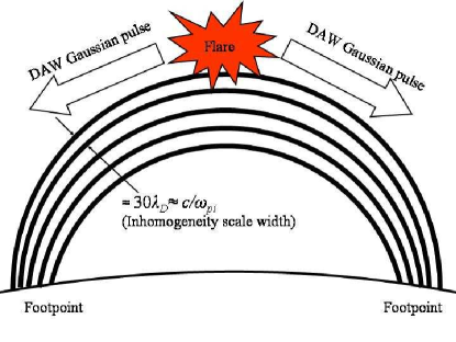
Figure 1: A conceptual sketch of the model. A solar flare launches DAW Gaussian pulses from the solar coronal loop apex which rush down towards the photospheric footpoints where X-rays are produced.

The general observational context of this work in outlined in Fig. 1, which shows that a solar flare at the solar coronal loop apex triggers DAWs Gaussian pulses which then propagate towards loop footpoints. There are possibilities of excitation of KAWs or IAWs by means of turbulent cascade Zharkova and Siversky (2011) or magnetic field-aligned currents i.e. essentially electron beams drifting with respect to stationary ions Chen and Wu (2012) or fast ion beam excitation Voitenko (1996). Chen et al. (2011) considered the situation when KAWs are excited by current (fluid) instability. The instability condition for this excitation by current is satisfied when the drift velocity, $v_{D}=0.1v_{A}$, and KAWs can efficiently grow. However, Chen et al. (2011) did not include the resonant excitation of DAWs by the inverse Landau damping because its instability condition requires a larger drift velocity, in general, larger than the Alfven velocity. Tsiklauri (2011); Bian and Kontar (2011) considered a different regime, where the importance of the Landau (Cerenkov) resonance for the particle acceleration and parallel electric field generation by the DAWs.

In our model (see Fig. 1) the transverse density (and temperature) inhomogeneity scale is of the order of $30$ Debye length ($\lambda_{D}$) that for the considered mass ratio $m_{i}/m_{e}=16$ corresponds to 0.75 ion inertial length $c/\omega_{pi}$. Possibility of existence of such thin loop threads, tens of cm wide, in the solar corona is debatable, based on loops observed with TRACE and SDO’s AIA. However, future high spatial resolution space missions, such as Solar Probe Plus and Solar Orbiter may shed light on the possible loop sub-structuring. Yet another shortcoming, partly associated with previous one, is the unrealistically small longitudinal scales considered. Our longest considered domain is $106.91$ m, which ideally should have been 100 Mm. Albeit, inability to resolve full kinetics and realistic spatial scales at the same time, plague all current particle-in-cell simulations.

We use EPOCH (Extendable Open PIC Collaboration) a multi-dimensional, fully electromagnetic, relativistic particle-in-cell code which was developed and is used by Engineering and Physical Sciences Research Council (EPSRC)-funded Collaborative Computational Plasma Physics (CCPP) consortium of 30 UK researchers (Arber et al., 2015). We use 2.5D version of the EPOCH code. The relativistic equations of motion are solved for each individual plasma particle. The code also solves Maxwell’s equations, with self-consistent currents, using the full component set of EM fields $E_{x},E_{y},E_{z}$ and $B_{x},B_{y},B_{z}$. EPOCH uses SI units. For the graphical presentation of the results time is normalised to $\omega_{\mathrm{pe}}^{-1}$. When visualizing the normalised results we use $n_{0}=10^{16}$ m^-3 in the least dense parts of the domain ($y=0$, $y=y_{max}$), which are located at the edges of the simulation domain (i.e. fix $\omega_{\mathrm{pe}}=5.64\times 10^{9}$ Hz radian on the domain edges). Here $\omega_{\mathrm{pe}}=\sqrt{n_{e}e^{2}/(\varepsilon_{0}m_{e})}$ is the electron plasma frequency, $n_{\alpha}$ is the number density of species $\alpha$ and all other symbols have their usual meaning. The x-size of the simulation box is different in different numerical runs, as stated in table 1. The considered x-range is $13200<x_{max}<20000$ grid points. $y_{max}=200$ grid points and is fixed in all runs. The four main runs are for the mass ratio $m_{i}/m_{e}=16$. This mass ratio value corresponds to the in the inertial Alfven wave (IAW) regime because plasma beta in this study is fixed at $\beta=2(v_{th,i}/c)^{2}(\omega_{pi}/\omega_{ci})^{2}=n_{0}(0,0)k_{B}T/(B_{0}^{2}/(2\mu_{0}))=0.02$. Thus $\beta=0.02<m_{e}/m_{i}=1/16=0.0625$; This is a reasonable compromise value that can be considered with the available computational resources. The grid unit size in the four runs is $\Delta=\lambda_{D}$, except for the Run1C where it is $\Delta=\sqrt{3}\lambda_{D}$. The latter is because we reduce the background plasma temperature three times and thus the Debye length decreases by $\sqrt{3}$. To keep the same length of domain, the factor of $\sqrt{3}$ in grid stretching is needed (to keep the same number of grids). For the four main runs $\lambda_{D}=v_{th,e}/\omega_{\mathrm{pe}}=5.345\times 10^{-3}$ m is the Debye length ($v_{th,e}=\sqrt{k_{B}T/m_{e}}$ is electron thermal speed). This makes the spatial simulation domain size of $x=[0,x_{max}]=[0,70.56-106.91m]$, $y=[0,y_{max}]=[0,1.069m]$. In the PIC code the velocity of particles is a continuous physical quantity, however when distribution function is calculated, this is sampled by a finite velocity (momentum) grid. Particle velocity space is resolved (i.e distribution functions produced in $V_{x},V_{y},V_{z}$ directions) with 100000 grid points with particle momenta in the range $\mp 1.5\times 10^{-21}$ kg m s^-1 or $\mp 3\times 10^{-21}$ kg m s^-1, depending on numerical run (see table 1).

We impose constant background magnetic field $B_{0x}=320.0$ Gauss along $x$-axis. This sets $\omega_{ce}/\omega_{\mathrm{pe}}=0.998$. Electron and ion temperature at the simulation box edge is also fixed at $T(0,0)=T_{e}(0,0)=T_{i}(0,0)=6\times 10^{7}$K, except for the Run1C where $T(0,0)=2\times 10^{7}$K. This in conjunction with $n_{0}(0,0)=10^{16}$ m^-3 makes plasma parameters similar to that of a dense flaring loops in the solar corona.

Figure 2: Plot of $n(y)/n(0)$ open diamonds and $T(y)/T(0)$ solid line at $t=0$ according to equations 1 and 2.

We consider a transverse to the background magnetic field variation of number density as following

$${n(y)}=1+3\exp\Biggl{[}-\left(\frac{y-y_{max}/2}{50\Delta}\right)^{6}\Biggl{]}\equiv f(y).$$ (1)

Equation 1 implies that in the central region (across the $y$ direction), the density is smoothly enhanced by a factor of 4, and there are the strongest density gradients having a width of about ${30\Delta}$ around the points $y=51.5\Delta$ and $y=148.5\Delta$, as can be seen in Fig. 2.

Fig. 2 shows $n(y)/n(0)$ open diamonds and $T(y)/T(0)$ solid line at $t=0$. This density behaviour represents the solar coronal loop. The background temperature of ions and electrons are varied accordingly

$${T_{i}(y)}/{T_{0}}={T_{e}(y)}/{T_{0}}=f(y)^{-1},$$ (2)

such that the thermal pressure remains constant. Because the background magnetic field along the $x$-coordinate is constant, the total pressure is also constant, ensuring the pressure balance. Note that flaring solar coronal loops are not such simple pressure-balanced structures. In reality during the flare there will be a magnetic energy release as a result of magnetic reconnection. It is commonly accepted that this will produce heat and super-thermal particles rushing down towards the sun. The point often over-looked is that this energy release results also in magnetic field reconfiguration launching Alfven waves too Fletcher and Hudson (2008). Inherent transverse inhomogeneity will create progressively smaller spatial scales via phase-mixing Tsiklauri et al. (2005). Our simplified initial configuration does not take into account complex nature of the flare magnetic energy release. To study wave dynamics in this idealized pressure-balanced structure seems a reasonable starting point, but it should be keep in mind that flaring solar coronal loops are far from the pressure balance.

The DAW is launched by three different means: (i) Run 1, with driving domain left edge, $x=1\Delta$, with the electric field as follows

$$E_{y}(1,y,t+\Delta t)=E_{y}(1,y,t)+E_{0}\exp\left(-\frac{(t-(30/\omega_{ci}))^{2}}{(12/\omega_{ci})^{2}}\right).$$ (3)

Here $E_{0}=1.4390\times 10^{6}$ V/m that corresponds to $0.6m_{e}\omega_{\mathrm{pe}}C_{A}(0,0)/e$ (for $m_{i}/m_{e}=16$). This produces the DAW pulse by electric field driving. (ii) Run 2, where we impose $B_{z}$ and $E_{y}$ Gaussian pulses

$$B_{z}=0.2B_{0}\exp\left(-\frac{(x-(30c/\omega_{pi}))^{2}}{(12c/\omega_{pi})^{2}}\right),\,E_{y}=B_{z}C_{A}(y)$$ (4)

at t=0; (iii) Run 3, where we impose $B_{z}$ and $E_{y}$ Gaussian pulses as in (ii), plus Alfvenic velocity perturbation $V_{z}=-C_{A}(y)B_{z}$; The latter is essentially achieved by including additional species of both electrons and ions with particle momentum drifts of $7.0336\times 10^{-23}$ and $1.1254\times 10^{-21}$ kg m s^-1, which correspond to $p_{e,i}=m_{e,i}C_{A}(0,0)/\sqrt{1-C_{A}(0,0)^{2}/c^{2}}$. For the mass ratio $m_{i}/m_{e}=16$ $C_{A}(0,0)/c=0.2494\approx 0.25$ and for $m_{i}/m_{e}=64$ $C_{A}(0,0)/c=0.1247\approx 0.125$. The additional species are localised in x-coordinate as following

$$n_{e,i}=0.2n_{0}\exp\left(-\frac{(x-(30c/\omega_{pi}))^{2}}{(12c/\omega_{pi})^{2}}\right).$$ (5)

We never include these additional species in any particle data visualisation, as only dynamics of background electrons and ions is shown. As will be shown below when discussing Run 3 such initial conditions achieve nearly perfect launch of single Gaussian pulse in the positive x-direction. While runs 1 and 2 suffer from the shortcoming that initial Gaussian pulse is split into two pulses with half-amplitude (positive and negative for run 1 and both positive for run 2) propagating in the opposite directions.

Table 1: Numerical runs details. PPC/TPS stands for particles-per-cell/total-particles-per-species in billions ($10^{9}$). $t_{end}$ is simulation end time in units of $\omega_{\mathrm{pe}}$. $p_{max}$ stands for the considered numerical momentum range $\mp p_{max}$ in units of $10^{-21}$ kg m s^-1.

Case	$n_{x}$	PPC/TPS	$t_{end}$	$p_{max}$	core$\times$hours	$m_{i}/m_{e}$
Run1	$13200$	$512/1.35$	$2406$	1.5	$192\times 74$	16
Run1H	$20000$	$340/1.36$	$9622$	3.0	$384\times 135$	64
Run2	$15000$	$512/1.54$	$2806$	1.5	$192\times 110$	16
Run3	$15000$	$256/0.77$	$2526$	1.5	$192\times 114$	16
Run1C	$13200$	$512/1.35$	$2406$	1.5	$192\times 71$	16

III Results

III.1 theoretical consideration

As discussed by Stasiewicz et al. (2000); McClements and Fletcher (2009) in the inertial regime ($\beta\ll m_{e}/m_{i}$) when Alfven perpendicular wavelength approaches the kinetic scales, electrostatic potential, $\phi$, and magnetic vector potential component along the background magnetic field $A_{x}$ satisfy the following equations

$$\left(1-\frac{c^{2}}{\omega_{\mathrm{pe}}^{2}}\nabla_{\perp}^{2}\right)\frac{\partial A_{x}}{\partial t}=-\frac{\partial\phi}{\partial x},$$ (6)

$$\frac{\partial A_{x}}{\partial x}=-\frac{1}{C_{A}(y)^{2}}\frac{\partial\phi}{\partial t},$$ (7)

where $\nabla_{\perp}^{2}=\partial^{2}_{yy}+\partial^{2}_{zz}$. Taking time derivative of equation 6 and then expressing $\partial^{2}\phi_{xt}$ from x-derivative of equation 7, one arrives at the master equation for $A_{x}$

$$\left[\partial^{2}_{tt}-C_{A}(y)^{2}\partial^{2}_{xx}\right]A_{x}=\left({c^{2}}/{\omega_{\mathrm{pe}}^{2}}\right)\partial^{2}_{yy}\partial^{2}_{tt}A_{x}.$$ (8)

Equation 8 left hand side is essentially the wave equation and the right hand side corresponds to a dispersion. As we will show below the pulse amplitude decrease is due to dispersive effects. It is worthwhile noting that Equation 8 if formally similar to the resistive MHD case, in particular equation (A.1) from Tsiklauri et al. (2003), with the following substitution $\eta\to(c/\omega_{\mathrm{pe}})^{2}$ and $\partial_{t}\to\partial^{2}_{tt}$. Also the following relation holds $\vec{B}=\nabla\times\vec{A}$.

We now introduce the following coordinates, that are co-moving with the wave, as well as slow (dispersion) time scale: $(x,y,z,t)\to(\xi,\bar{y},\bar{z},\tau)$: $\xi=x-C_{A}(y)t$, $\bar{y}=y$, $\bar{z}=z$, and $\tau=\varepsilon t$ (with $\varepsilon\ll 1$). The derivatives using the new coordinate system are:

$$\frac{\partial}{\partial x}=\frac{\partial}{\partial\xi},\,\,\,\,\frac{\partial}{\partial z}=\frac{\partial}{\partial\bar{z}},$$ (9)

$$\frac{\partial}{\partial y}=\frac{\partial}{\partial\bar{y}}-C_{A}^{\prime}(y)t\frac{\partial}{\partial\xi},$$ (10)

$$\frac{\partial}{\partial t}=-C_{A}(y)\frac{\partial}{\partial\xi}+\varepsilon\frac{\partial}{\partial\tau}.$$ (11)

Here, prime denotes a derivative over $y$. Using the co-moving variables and their derivatives, the leading term on the left hand side of equation 8 is $-2\varepsilon C_{A}(y)\partial^{2}_{\tau\xi}A_{x}$. On the right hand side we have

$$\frac{c^{2}}{\omega_{\mathrm{pe}}^{2}}\left(\frac{\partial^{2}}{\partial\bar{y}^{2}}-2C^{\prime}_{A}(y)t\frac{\partial^{2}}{\partial\bar{y}\partial\xi}+C^{\prime}_{A}(y)^{2}t^{2}\frac{\partial^{2}}{\partial\xi^{2}}\right)\times$$

$$\left(\varepsilon^{2}\frac{\partial^{2}}{\partial\tau^{2}}-2\varepsilon C_{A}(y)t\frac{\partial^{2}}{\partial\tau\partial\xi}+C_{A}(y)^{2}\frac{\partial^{2}}{\partial\xi^{2}}\right).$$ (12)

Thus keeping the largest terms from the each bracket, i.e. with $t^{2}$ in the first (because we consider large times $t/t_{Alfven}\gg 1$) and one without $\varepsilon$ in the second bracket, the leading term is $(c^{2}/\omega_{\mathrm{pe}}^{2})C_{A}(y)^{2}\partial^{2}_{\xi\xi}[C^{\prime}_{A}(y)^{2}(\tau/\varepsilon)^{2}\partial^{2}_{\xi\xi}A_{x}]$. Performing integration over $\xi$ and introduction of yet another auxiliary variable, $s=(c^{2}/\omega_{\mathrm{pe}}^{2})C^{\prime}_{A}(y)^{2}C_{A}(y)\tau^{3}/(6\varepsilon^{3})=(c^{2}/\omega_{\mathrm{pe}}^{2})C^{\prime}_{A}(y)^{2}C_{A}(y)t^{3}/6$, we obtain the following equation for $A_{x}$:

$$\partial_{s}A_{x}=-\partial^{3}_{\xi\xi\xi}A_{x}.$$ (13)

Equation 13 is the linear Korteweg de Vries (KdV) equation. Non-linear KdV equation describes propagation of solitons where non-linearity (usual $6A_{x}\partial_{\xi}A_{x}$ term) provides wave-overturning, while dispersion (the $\partial^{3}_{\xi\xi\xi}A_{x}$ term) causes spatial spreading and appearance of wave-forms on the left side of the domain (see figure 7, bottom left panel). It is quite natural that the dispersive term $\partial^{3}_{\xi\xi\xi}A_{x}$ appears in the equation describing dispersive (inertial) Alfven wave. The relevance here is also in the $c/\omega_{\mathrm{pe}}$ term which replaces the resistivity $\eta$, compared to the resistive MHD, represents electron inertial length. We note that in the resistive MHD phase-mixing the equivalent to equation 13 is as following

$$\partial_{s}B_{y}=\partial^{2}_{\xi\xi}B_{y},$$ (14)

which is equation (A.3) from Tsiklauri et al. (2003). Equation 14 is the diffusion equation, because in the resistive MHD magnetic field diffuses through plasma. In the homogeneous plasma regions the Alfvenic, Gaussian pulse amplitude diffuses as $B_{y}(t)\propto t^{-1/2}$ (Tsiklauri, 2016), while due to the effect of phase mixing, in the inhomogeneous regions the diffusion is faster, $B_{y}(t)\propto t^{-3/2}$ (Tsiklauri et al., 2003).

In order to solve liner KdV equation 13 we employ non-unitary Fourier forward and inverse transforms

$$\hat{f}(k)=\int_{-\infty}^{\infty}f(x)e^{-ikx}dx,$$

$$f(x)=\frac{1}{2\pi}\int_{-\infty}^{\infty}\hat{f}(k)e^{ikx}dk.$$ (15)

Substituting equation 15 into 13 with the initial (at $s=0$ instant) condition, $A_{x}(\xi,0)=\exp(-\xi^{2})$, we obtain

$$A_{x}(\xi,s)=\frac{1}{2\pi}\int_{-\infty}^{\infty}\hat{A}_{x}(k)e^{ik^{3}s}e^{ik\xi}dk=$$

$$\frac{1}{2\sqrt{\pi}}\int_{-\infty}^{\infty}e^{-k^{2}/4+ik^{3}s+ik\xi}dk.$$ (16)

We used here the fact that Fourier transform of simple Gaussian $\exp(-\xi^{2})$ is also a Gaussian in k-space $\sqrt{\pi}\exp(-k^{2}/4)$. For large times $t,\tau,s\to\infty$, as done in equation (A.5) from Tsiklauri et al. (2003), from the triple sum under the exponent in equation 16 we keep the largest term $ik^{3}s$. Noting that

$$\int_{-\infty}^{\infty}e^{ik^{3}s}dk=-\frac{2\pi}{\Gamma(-1/3)}s^{-1/3},$$ (17)

and using equation 16, we obtain asymptotic (the large times) solution for $A_{x}$ as following

$$A_{x}(\xi,s)=-\frac{\sqrt{\pi}}{\Gamma(-1/3)}s^{-1/3}.$$ (18)

Here $\Gamma(-1/3)=-4.06235$ is the Gamma-function. Thus the main conclusion of this sub-section is that as equation 18 asserts, Gaussian pulse amplitude scales in time as $\propto s^{-1/3}\propto t^{-1}$.

III.2 numerical validation

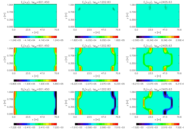
Figure 3: Contour (intensity) plots of the following physical quantities at times indicated at individual panels: (top row) $E_{x}(x,y)$, (middle row) $E_{y}(x,y)$, and (bottom row) $B_{z}(x,y)$.

Fig. 3 presents the numerical simulation results for the electromagnetic fields for Run 1. In Run 1 we output 20, equally spaced in time data snapshots and each column in the figure corresponds to 5th, 10th, 20th snapshot. The 20th snapshot corresponds to $t=2406\omega_{\mathrm{pe}}=150\omega_{ci}$. The other parameters of this run are indicated in Table 1. We see from Fig. 3 the usual phase mixing picture, i.e. $E_{y}$ and $B_{z}$ pulses are excited that propagate in positive and negative x-direction, because the electric field driving according to equation 3 is unable to excite a clear eigen-mode of the system propagating on in the positive x-direction. As throughout the paper we use periodic boundary conditions, the pulse that propagates to the left, i.e. in the negative x-direction, re-appears on the right side of the domain and propagates to the left. The pulse that propagates to the right (positive x-direction) is also clearly present. Because according to equation 1 the density is smoothly enhanced by a factor of 4 in the middle of y-coordinate range, phase speed of the wave is slower there, as roughly $V_{\rm phase}\approx B_{0}/\sqrt{\mu_{0}m_{i}n_{0}}=C_{A}(y)$. Thus the front phase-mixes and creates transverse gradients. It is in the region of these gradients, near the points $y=51.5\Delta$ and $y=148.5\Delta$, $E_{x}$, the parallel electric field is generated. As seen in the middle and right panels of top row of Fig. 3, the generated $E_{x}$ is clearly seen near $y=148.5\Delta$ (but not near $y=51.5\Delta$ – this is probably due to small number of contour levels used to reduce the figure disk space). The similar type behaviour, but for the harmonic Alfvenic wave was seen in Tsiklauri et al. (2005); Tsiklauri and Haruki (2008), in 2.5D geometry and 3D geometry in Tsiklauri (2012).

Figure 4: Scaling of $B_{z}$ DAW pulse amplitude with time. The dashed line is $B_{z}^{*}=\max(B_{z}(x,y=51\Delta))$, which tracks the amplitude in the strongest density gradient point. Solid line is $\max(B_{z}(x,y=1\Delta))$ which tracks the amplitude away from the density gradient. The triangles show the analytical (numerically fitted) scaling law $B_{z}^{*}\propto t^{-1.1}$.

Fig. 4 shows the scaling of $B_{z}$ DAW pulse amplitude with time. The dashed line is $B_{z}^{*}=\max(B_{z}(x,y=51\Delta))$ for the right propagating pulse, which tracks the amplitude in the strongest density gradient point. Solid line is $\max(B_{z}(x,y=1\Delta))$ which tracks the amplitude away from the density gradient. This shows no decrease (the solid line stays at the same level) meaning that there is no significant amplitude decrease of the pulse away from the transverse density gradient regions. The triangles show the analytical (numerically fitted) scaling law $B_{z}^{*}\propto t^{-1.1}$. The fitting is done using IDL’s poly_fit routine, and employing the last 10 out of 20 total time sampling points. The poly_fit routine is used as following: $B_{z}=e^{r}_{0}t^{r_{1}}$ where $r_{0}$ and $r_{1}$ the fit parameters. Further we use $\ln B_{z}=r_{0}+r_{1}\ln t$. Then using the first order polynomial fit of the form $f(x)=a_{0}+a_{1}x$ in poly_fit routine where $e^{r}_{0}=a_{0}$ and $r_{1}=a_{1}$ provides the fit. Thus we show that in the kinetic regime the scaling law for the Gaussian pulse amplitude decay in time is not the same as in MHD ($B_{z}\propto t^{-3/2}$ Tsiklauri (2016)), namely, $B_{z}\propto t^{-1}$. This is due to the fact that the diffusion equation is replaced by the linear KdV equation. It is worthwhile noting that performing similar fit to the other strongest gradient point $B_{z}^{*}=\max(B_{z}(x,y=148\Delta))$, not shown here, produces the best fit of $B_{z}^{*}\propto t^{-1.0}$. Thus the results for both strongest gradient points are consistent.

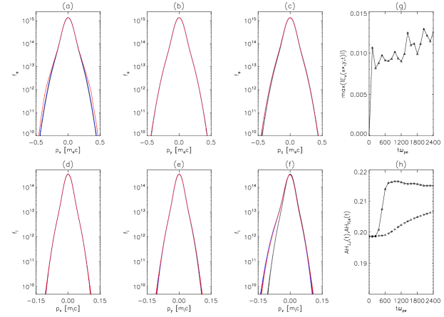
Figure 5: Time evolution of electron and ion velocity distribution functions versus velocity $x,y$ and $z$ components on a log-linear plot: (a) $f_{e}(p_{x},t=0)$ black (inner) curve, $f_{e}(p_{x},t=t_{end}/2)$ blue and $f_{e}(p_{x},t=t_{end})$ red (outer) curve, (b) $f_{e}(p_{y},t=0)$ black curve, $f_{e}(p_{y},t=t_{end}/2)$ blue and $f_{e}(p_{y},t=t_{end})$ red curve, (c) $f_{e}(p_{z},t=0)$ black curve, $f_{e}(p_{z},t=t_{end}/2)$ blue and $f_{e}(p_{z},t=t_{end})$ red curve, (d) $f_{i}(p_{x},t=0)$ black curve, $f_{i}(p_{x},t=t_{end}/2)$ blue and $f_{i}(p_{x},t=t_{end})$ red curve, (e) $f_{i}(p_{y},t=0)$ black curve, $f_{i}(p_{y},t=t_{end}/2)$ blue and $f_{i}(p_{y},t=t_{end})$ red curve, (f) $f_{i}(p_{z},t=0)$ black curve, $f_{i}(p_{z},t=t_{end}/2)$ blue and $f_{i}(p_{z},t=t_{end})$ red curve. Time evolution (at 20 time intervals between $t=0$ and $t=t_{end}$) of the following: (g) $\max(|E_{x}(x=51\Delta,y,t|)$, triangles connected with a solid curve and (h) $AH_{||,e}$ index, diamonds connected with dashed curve, according to equation 19, $AH_{\perp,i}$ index, triangles connected with a solid curve, according to equation 20. This figure pertains to the numerical Run 1.

Fig. 5 shows electron (panels a–c) and ion (panels d–f) distribution function dynamics for Run 1. It also shows, in panel (g), the time evolution (at 20 time intervals between $t=0$ and $t=t_{end}$) of $max(|E_{x}(x=51\Delta,y,t|)$ plotted with triangles connected with a solid curve. In panel (h) $AH_{||,e}$ index is plotted with diamonds connected with dashed curve, according to equation 19, and $AH_{\perp,i}$ index plotted with triangles connected with a solid curve, according to equation 20. We deduce from panel (a) that the two bumps in the parallel electron distribution function (for negative and positive velocities) can be understood by a Landau resonance because it corresponds to phase speed of the DAW $V_{phase}=0.2494c$. This is similar result to to our earlier works Tsiklauri et al. (2005); Tsiklauri and Haruki (2008); Tsiklauri (2011, 2012) for the harmonic Alfven wave. However, what is different (e.g. compare figure 5 to figure 3 from Tsiklauri (2011)) is that electric field is twice as weak (panel (g)) and particle acceleration is much less efficient. A more rigorous proof that indeed we deal with the Landau resonance is presented below when discussing Run1H. We quantify the particle acceleration by introducing the following quantities:

$$AH_{\parallel,e}(t)=\frac{\int_{|v_{x}|>\langle v_{th,e}\rangle}^{\infty}f_{e}(v_{x},t)dv_{x}}{\int_{-\infty}^{\infty}f_{e}(v_{x},0)dv_{x}},$$ (19)

$$AH_{\perp,i}(t)=\frac{\int_{|v_{\perp}|>\langle v_{th,i}\rangle}^{\infty}f_{i}(v_{\perp},t)dv_{\perp}}{\int_{-\infty}^{\infty}f_{i}(v_{\perp},0)dv_{\perp}},$$ (20)

where $f_{e,i}$ are electron or ion velocity distribution functions and $<>$ brackets denote average over y-coordinate, because temperature and density vary across y-coordinate. These definitions effectively provides the fraction (the percentage) of super-thermal electrons and ions. We gather from panel (h) that $AH_{||,e}$ index starts from $0.199$ and stops at $0.207$, meaning that the difference $0.207-0.199=0.008\approx 0.01$, i.e. one percent of electrons are accelerated above thermal speeds. For ions this number is about twice as large ($\approx 2\%$) due to negative $p_{z}$ momenta in panel (f).

Figure 6: Left panel’s solid and dashed curves are the total (particles plus EM fields) and particle energies, normalized on initial values, respectively. Right panel shows EM field energy normalized on its initial value.

Fig. 6 shows that the total energy has a small, 0.6%, increase. This is a tolerable error due to the well-know numerical heating inherent to PIC codes. The all three energies go up until about $t=800\omega_{\mathrm{pe}}$ this corresponds to the timescale of growth of the electric field according to equation 3. Then particle energy continues to grow much slowly while particles are accelerated via collisionless Landau damping. The electromagnetic energy decreases after $t=800\omega_{\mathrm{pe}}$ which means that particle acceleration is on the expense of electromagnetic energy decrease.

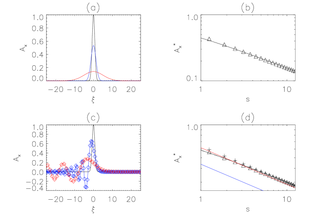
Figure 7: Time evolution of Gaussian pulse, $A_{x}(\xi,0)=\exp(-\xi^{2})$: panel (a) according to the diffusion equation 14. Black curve is for $A_{x}(\xi,s=0)$, blue for $A_{x}(\xi,s=0.625)$ and red for $A_{x}(\xi,s=12.5)$. Panel (b) is a log-log plot of $A_{x}^{*}=\max(A_{x}(\xi,s))$ at different times $s$, showing evolution according to the diffusion equation 14 (with $B_{y}$ replaced by $A_{x}$). The solid line is numerical solution of the code and triangles represent numerical fit $s^{-0.488}$ performed using IDL’s poly-fit routine (see text for details). Panel (c) shows evolution of $A_{x}$ according to the KdV equation 13. In addition to black, blue and red lines, which represent the numerical code solution, we also plot analytical solution with open diamonds according to real part of equation 16, i.e. $A_{x}(\xi,s)=\frac{1}{2\sqrt{\pi}}\int_{-\infty}^{\infty}e^{-k^{2}/4}\cos(k^{3}s+k\xi)dk$ using IDL’s int-tabulated routine. Panel (d) is showing a log-log plot of $A_{x}^{*}=\max(A_{x}(\xi,s))$ according to the KdV equation 13. The solid black line corresponds to numerical solution of the code. In addition, dashed line that fully overlaps the solid line represents the same analytical solution using IDL’s int-tabulated routine. The triangles show represent numerical fit $s^{-0.305}$, using IDL’s poly-fit routine to the numerical code solution. The crosses represent the similar fit but to the analytical solution and the fit yields $s^{-0.332}$. Blue line is according to equation 18 with $s^{-1/3}$. The red line is the same but with additional factor $\sqrt{2}$ which fits data better.

Fig. 7 presents time evolution of Gaussian pulse, $A_{x}(\xi,0)=\exp(-\xi^{2})$. The panel (a) is the evolution according to the diffusion equation 14 (with $B_{y}$ replaced by $A_{x}$) for the numerical code versification purposes. Black curve is for $A_{x}(\xi,s=0)$, blue for $A_{x}(\xi,s=0.625)$ and red for $A_{x}(\xi,s=12.5)$. Note how the diffusive spatial spread (widening of the pulse) progressively becomes evident. The simple numerical code and Interactive Data Language (IDL) routines are available from http://ph.qmul.ac.uk/~tsiklauri/toyama_2016. The code solves the diffusion and KdV equations using 4th order Runge-Kutta time step. It uses 4th order centered differencing for the second order spatial derivative in the diffusion equation and 2nd order centered differencing for the third order spatial derivative in the KdV equation using Table 1 from Fornberg (1988). The code has domain size of $\xi=[-250,250]$ and end simulation times is $t=12.5$. The spatial domain has 20000 points. Panel (b) is a log-log plot of $A_{x}^{*}=\max(A_{x}(\xi,s))$ at different times $s$, showing evolution according to the diffusion equation 14 (with $B_{y}$ replaced by $A_{x}$). The solid line is numerical solution of a code and triangles represent numerical fit $s^{-0.488}$, using IDL’s poly_fit routine, and employing the last 6 out of 20 total time sampling points. In the homogeneous plasma regions the Alfvenic, Gaussian pulse amplitude diffuses as $B_{y}(t)\propto t^{-1/2}$ Tsiklauri (2016). We see that solution of the diffusion equation is handled very well by the code, as $-0.488$ is nearly $-0.5$. We use the last 6 points because the predicted scaling becomes progressively better for increasing time. Panel (c) shows evolution of $A_{x}$ according to the KdV equation 13. In addition to black, blue and red lines, which represent the numerical code solution, we also plot analytical solution with open diamonds according to real part of equation 16, i.e. $A_{x}(\xi,s)=\frac{1}{2\sqrt{\pi}}\int_{-\infty}^{\infty}e^{-k^{2}/4}\cos(k^{3}s+k\xi)dk$ using IDL’s int_tabulated routine. The routine uses domain size of $k=[-250,250]$ with 40000 point discretization. We see that the pulse amplitude decreases but also the dispersion creates wave-like pattern in the negative $\xi$ region. This is the expected behaviour and we see similar pattern in PIC simulations too. The diamonds are plotted with much less than actual grid number points to aid the visualization (we plot every 20th point for blue diamonds and every 50th for the red). To a plotting precision the match between the numerical and analytical solutions is obvious. Panel (d) shows a log-log plot of $A_{x}^{*}=\max(A_{x}(\xi,s))$, according to the KdV equation 13. The solid black line corresponds to numerical solution of the code. In addition, dashed line that fully overlaps the solid line represents the analytical solution $A_{x}(\xi,s)=\frac{1}{2\sqrt{\pi}}\int_{-\infty}^{\infty}e^{-k^{2}/4}\cos(k^{3}s+k\xi)dk$ using IDL’s int_tabulated routine. The triangles represent numerical fit $s^{-0.305}$, using IDL’s poly_fit routine to the numerical code solution, and employing the last 6 out of 20 total time sampling points. Crosses represent the similar fit but now applied to the analytical solution. The fit yields $s^{-0.332}$. Again, the poly_fit routine is used in the following manner: We start from $A_{x}=e^{r}_{0}s^{r_{1}}$ where $r_{0}$ and $r_{1}$ the fit parameters. Then $\ln A_{x}=r_{0}+r_{1}\ln s$. Using first order polynomial fit of the form $f(x)=a_{0}+a_{1}x$ in poly_fit routine where $e^{r}_{0}=a_{0}$ and $r_{1}=a_{1}$ gives the desired fitting. Blue line shows the solution according to equation 18. The red line is the solution according to equation 18 but with additional factor $\sqrt{2}$ which fits data better. Thus we conclude that as equation 18 shows, the Gaussian pulse amplitude scales in time according to KdV equation 13 as $\propto s^{-1/3}\propto s^{-0.3333}\propto t^{-1}$. While the homogeneous diffusion equation solution scales as $\propto s^{-1/2}$.

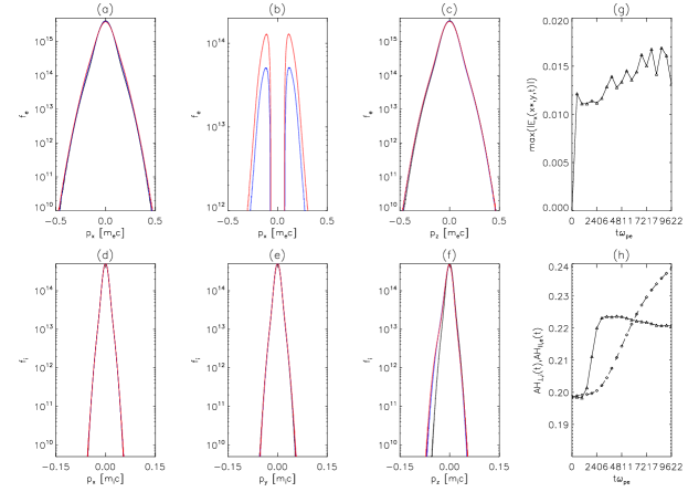
Figure 8: As in Fig. 5, but for the Run1H with mass ratio 64. Here we replaced panel (b) with $f_{e}(p_{x},t=t_{end}/2)-f_{e}(p_{x},t=0)$ blue and $f_{e}(p_{x},t=t_{end})-f_{e}(p_{x},0)$ red curves, in oder to emphasize the difference between the distribution functions at different times.

The Run1H corresponds to keeping everything the same is in Run 1 but making heavier ions by factor of 4, i.e. now the mass ratio is $m_{i}=m_{e}=64$. This makes the phase speed of DAW twice as small $V_{phase}/c\approx 0.125$. Fig. 8 is similar to Fig. 5, but for the Run1H. It is barely visible that the two bumps in the parallel to the field distribution function, $f_{e}(p_{x})$, have now shifted from 0.25 to 0.125. Thus we replaced panel (b) with $f_{e}(p_{x},t=t_{end}/2)-f_{e}(p_{x},t=0)$ blue and $f_{e}(p_{x},t=t_{end})-f_{e}(p_{x},0)$ red curve, in oder to stress the difference between the distribution functions at different times. It is evident the the bumps are now near $\pm 0.125$. This proves that the acceleration of the particles is due to Landau damping. Similar conclusion also was reached before, when the harmonic DAW was considered in Tsiklauri et al. (2005); Tsiklauri and Haruki (2008), in 2.5D geometry and 3D geometry in Tsiklauri (2012). Other noteworthy feature is the for Run1H we see more efficient particle acceleration, as $AH_{||,e}$ index starts from $0.199$ and stops at $0.238$, meaning that $0.238-0.199=0.039\approx 0.04$, i.e. four percent of electrons are accelerated above thermal speeds. Thus four times more massive ions result in four times more efficient electron acceleration. Of course, this is still far below of requirement to produce X-rays in solar flares, where $\approx 50$ percent of electrons are accelerated. It is unclear what the results would be for the realistic mass ratio of $m_{i}/m_{e}=1836$.

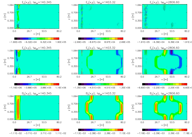
Figure 9: As in Fig. 3 but for the run 2.

Fig. 9 presents the numerical simulation results for the electromagnetic fields for Run 2. In Run 2 we also output 20, equally spaced in time data snapshots and each column in the figure corresponds to 1st, 10th, 20th snapshot. $E_{y}$ and $B_{z}$ show again phase-mixed behaviour, but the new type of initial conditions according to equation 4 now only result in a single $B_{z}$ positive pulse being split into two positive pulses with half amplitude travelling in opposite directions. In the case of Run 1, the pulse the moved to the right was positive while one moving to the left was negative. Parallel electric field is also generated in the transverse density gradient regions and now seen about around $y=51.5\Delta$ and $y=148.5\Delta$.

Figure 10: As in Fig. 4 but for the run 2. Here the numerical fit produces the following scaling law $B_{z}^{*}\propto t^{-0.75}$.

Fig. 10 shows the pulse amplitude dynamics as in Fig. 4 but for the run 2. In this case the numerical fit produces the scaling law of $B_{z}^{*}\propto t^{-0.75}$. This exponent is note quite $-1$ but reasonably close. The discrepancy could be due to the fact the the excited pulse is not quite an eigen-mode of the system and also the non-linearity could play role as the pulse amplitude is $20\%$, while the $B_{z}^{*}\propto t^{-1}$ is according to the linear KdV equation.

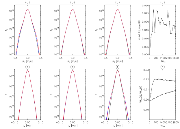
Figure 11: As in Fig. 5 but for the run 2.

There are many similarities of Fig. 11 to Fig. 5, except that widening of the distribution function for ions in $p_{z}$ direction (panel f) is now symmetric.

Figure 12: As in Fig. 6 but for the run 2.

In Fig. 12, compared to Fig. 6, the following modifications can be observed: because there is no continuous energy input into the system, and we rather deal with initial value problem according to equation 4, there is monotonous increase in particle energy, while electromagnetic energy energy does not increase and it only decreases. The total energy line is nearly flat this due to the fact that the energy error is 0.0009%.

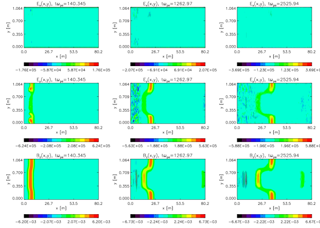
Figure 13: As in Fig. 3 but for the run 3.

Run 3 is our best attempt to launch a single Gaussian pulse that propagates in the positive x-direction. This is achieved by the initial condition specified above. In Fig. 13 we plot time evolution of phase mixed electromagnetic components $E_{y}$ and $B_{z}$ in a similar manner as in Fig. 3. We see from these panels that a single, Gaussian pulse is excited moving to the right (positive x-direction), only a minor backwards propagating pulse is visible in two bottom right panels near $x=80$ and $x=70$.

Figure 14: As in Fig. 4 but for the run 3. Here the numerical fit produces the following scaling law $B_{z}^{*}\propto t^{-0.76}$.

In Fig. 14 we plot the pulse amplitude dynamics as in Fig. 4 but for the run 3. In this case the numerical fit produces the scaling law of $B_{z}^{*}\propto t^{-0.76}$. Again, this exponent is note quite $-1$ but tolerably close.

Figure 15: As in Fig. 5 but for the run 3.

Fig. 15 panel (a) shows that as the time progresses the pump in the parallel electron distribution function develops is single pump corresponding to the positive velocity of the Gaussian pulse $V_{phase}/c=0.25$. We explain this by the fact the in Run 3 only one pulse is present that moves to positive x-direction. This is an interesting result partly because now we see bump only in the positive velocities, contrary to our earlier works Tsiklauri et al. (2005); Tsiklauri and Haruki (2008); Tsiklauri (2011, 2012). This serves a further proof that the particle acceleration is via Landau resonance damping.

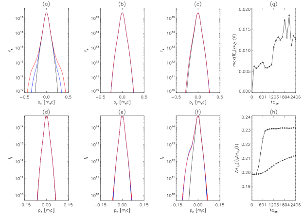
Figure 16: As in Fig. 5 but for the run 1C.

For run 3 the behaviour of the energies is similar to run 1, so no shown here – particle energy increases on the expense of the decrease of magnetic energy as the pulse damps. The total energy line is nearly flat this due to the fact that the energy error is 0.02%.

In Figure 16 we plot distribution function time evolution for Run1C. It is worthwhile to note the wider spread of red curve in panel (a) compared to panel (a) from Figure 5. This means that in cooler background plasma with $T=2\times 10^{6}$ (note that all other runs in this work have three times higher temperature of $T=6\times 10^{6}$). We gather from panel (h) that $AH_{||,e}$ index starts from $0.199$ and stops at $0.212$, meaning that $0.013$, i.e. 1.3% of electrons are accelerated above thermal speeds. For ions this number is about three times as large ($0.231-0.199\approx 3.2\%$).

IV Conclusions

We have advanced the knowledge of dynamics of Alfven waves and associated particle acceleration in the inhomogeneous space and solar plasmas by considering new type of DAW in a form of the Gaussian pulses. The latter are more appropriate for solar flares, as the flare is impulsive in its nature. The new results can be summarised as following: (i) Our linear analytical model makes a prediction that the pulse amplitude decrease is described by the linear KdV equation. (ii) The numerical and analytical solution of the linear KdV equation shows the pulse amplitude damping in time as $t^{-1}$, which is corroborated by full PIC simulations. (iii) We also prove that the electron acceleration is due to collisionless Landau damping. However, we would like to stress that the pulse amplitude decrease (the $t^{-1}$ scaling law) is due to dispersive effects. In effect, Section 3.1 shows that the phase-mixing leads to the dispersion, described by KdV equation, without resorting to the damping and wave-particle resonance. The dynamics of the particle distribution function in Section 3.2 shows that the particle resonance is with the phase-mixed waves which have the phase speed of the DAW pulse. (iv) We show that reducing background plasma temperature yields more efficient particle acceleration. (v) When we considered four times more massive ions with $m_{i}/m_{e}=64$, compared to the most runs in this study with $m_{i}/m_{e}=16$, this resulted in four times more efficient electron acceleration i.e. 4%. At this stage it is impossible for us to simulate the realistic mass ratio of $m_{i}/m_{e}=1836$ due to the computational limitations. Thus the jury is still out in the issue of feasibility of efficient electron acceleration by means of Gaussian, Alfvenic pulses. It should be noted that the issue of scaling of the generated $E_{\parallel}$ and hence the particle acceleration with the mass ratio has been investigated before Tsiklauri (2007) for the case of harmonic DAW. Ref.Tsiklauri (2007) proved that the minimal model required to reproduce previous kinetic results on $E_{\parallel}$ generation is the two-fluid, cold plasma approximation in the linear regime. Ref.Tsiklauri (2007) established that amplitude attained by $E_{\parallel}$ decreases linearly as the inverse of the mass ratio $m_{i}/m_{e}$ , i.e. $E_{\parallel}\propto 1/m_{i}$ . This result contradicts the earlier works Génot et al. (2004); Gét et al. (1999) in that the cause of $E_{\parallel}$ generation is the polarization drift of the driving wave, which scales as $E_{\parallel}\propto m_{i}$. Increase in mass ratio does not have any effect on the final parallel (magnetic field aligned) speed attained by electrons. However, parallel ion velocity decreases linearly with the inverse of the mass ratio $m_{i}/m_{e}$ , i.e. the parallel velocity ratio of electrons and ions scales directly as $m_{i}/m_{e}$. These were interpreted as follows: (i) ion dynamics plays no role in the $E_{\parallel}$ generation; (ii) decrease in the generated parallel electric field amplitude with the increase of the mass ratio $m_{i}/m_{e}$ is caused by the fact that the harmonic driving frequency $\omega_{d}=0.3\omega_{ci}\propto 1/m_{i}$ is decreasing, and hence the electron fluid can effectively ’short-circuit’ (recombine with) the slowly oscillating ions, hence producing smaller $E_{\parallel}$ which also scales exactly as $1/m_{i}$. Evidently, the same argument does not apply when harmonic DAW is replaced by the Gaussian pulse, which has no ”driving frequency” associated with it. Thus, further work is needed to investigate the scaling of the particle acceleration with the mass ratio.

Yet another issue that needs to be mentioned is the fact that flaring solar coronal plasma has plasma beta possibly close to unity ($\beta=p_{gas}/(B^{2}/2\mu_{0})\approx 1\gg m_{e}/m_{i}$) Aschwanden (2005). Whereas in our work most numerical runs are done for $\beta=0.02<m_{e}/m_{i}=1/16=0.0625$ and one run with Thus $\beta=0.02>m_{e}/m_{i}=1/64=0.0156$. We would like to remark that plasma conditions where the flare occurs and DAW propagate can be quite different. Once DAW leave the flare cite with $\beta\approx 1$ after their excitation, when rushing towards the footpoints, as sketched in Figure 1, they will be moving through plasma with $\beta\ll 1$. As already stated above, a separate study needs to be conducted how particle acceleration efficiency scales with the mass ratio, i.e. different relations between $\beta$ and $m_{e}/m_{i}$.