Towards a Constructive Version of Banaszczyk’s Vector Balancing Theorem

Abstract

An important theorem of Banaszczyk (Random Structures & Algorithms ‘98) states that for any sequence of vectors of $\ell_{2}$ norm at most $1/5$ and any convex body $K$ of Gaussian measure $1/2$ in $\mathbb{R}^{n}$, there exists a signed combination of these vectors which lands inside $K$. A major open problem is to devise a constructive version of Banaszczyk’s vector balancing theorem, i.e. to find an efficient algorithm which constructs the signed combination.

We make progress towards this goal along several fronts. As our first contribution, we show an equivalence between Banaszczyk’s theorem and the existence of $O(1)$-subgaussian distributions over signed combinations. For the case of symmetric convex bodies, our equivalence implies the existence of a universal signing algorithm (i.e. independent of the body), which simply samples from the subgaussian sign distribution and checks to see if the associated combination lands inside the body. For asymmetric convex bodies, we provide a novel recentering procedure, which allows us to reduce to the case where the body is symmetric.

As our second main contribution, we show that the above framework can be efficiently implemented when the vectors have length $O(1/\sqrt{\log n})$, recovering Banaszczyk’s results under this stronger assumption. More precisely, we use random walk techniques to produce the required $O(1)$-subgaussian signing distributions when the vectors have length $O(1/\sqrt{\log n})$, and use a stochastic gradient ascent method to implement the recentering procedure for asymmetric bodies.

1 Introduction

Given a family of sets $S_{1},\dots,S_{m}$ over a universe $U=[n]$, the goal of combinatorial discrepancy minimization is to find a bi-coloring $\chi:U\rightarrow\{-1,1\}$ such that the discrepancy, i.e. the maximum imbalance $\max_{j\in[m]}|\sum_{i\in S_{j}}\chi(i)|$, is made as small as possible. Discrepancy theory, where discrepancy minimization plays a major role, has a rich history of applications in computer science as well as mathematics, and we refer the reader to [22, 11, 12] for a general exposition.

A beautiful question regards the discrepancy of sparse set systems, i.e. set systems in which each element appears in at most $t$ sets. A classical theorem of Beck and Fiala [8] gives an upper bound of $2t-1$ in this setting. They also conjectured an $O(\sqrt{t})$ bound, which if true would be tight. An improved Beck-Fiala bound of $2t-\log^{*}t$ was given by Bukh [10], where $\log^{*}t$ is the iterated logarithm function in base $2$. Recently, it was shown by Ezra and Lovett [15] that a bound of $O(\sqrt{t\log t})$ holds with high probability when $m\geq n$ and each element is assigned to $t$ sets uniformly at random. The best general bounds having sublinear dependence in $t$ currently depend on $n$ or $m$. Srinivasan [30] used Beck’s partial coloring method [7] to give a bound of $O(\sqrt{t}\log\min\left\{n,m\right\})$. Using techniques from convex geometry, Banaszczyk [2] proved a general result on vector balancing (stated below) which implies an $O(\sqrt{t\log\min\left\{n,m\right\}})$ bound.

The proofs of both Srinivasan’s and Banaszczyk’s bounds were non-constructive, that is, they provided no efficient algorithm to construct the guaranteed colorings, short of exhaustive enumeration. In the last 6 years, tremendous progress has been made on the question of matching classical discrepancy bounds algorithmically. Currently, essentially all discrepancy bounds proved using the partial coloring method, including Srinivasan’s, have been made constructive [4, 21, 17, 27, 14]. Constructive versions of Banaszczyk’s result have, however, proven elusive until very recently. In recent work [5], the first and second named authors jointly with Bansal gave a constructive algorithm for recovering Banaszczyk’s bound in the Beck-Fiala setting as well as the more general Komlós setting. An alternate algorithm via multiplicative weight updates was also given recently in [19]. However, finding a constructive version of Banaszczyk’s more general vector balancing theorem, which has further applications in approximating hereditary discrepancy, remains an open problem. This theorem is stated as follows:

Theorem 1 (Banaszczyk [2]).

Let $v_{1},\dots,v_{n}\in\mathbb{R}^{m}$ satisfy $\|v_{i}\|_{2}\leq 1/5$. Then for any convex body $K\subseteq\mathbb{R}^{m}$ of Gaussian measure at least $1/2$, there exists $\chi\in\left\{-1,1\right\}^{n}$ such that $\sum_{i=1}^{n}\chi_{i}v_{i}\in K$.

The lower bound $1/2$ on the Gaussian measure of $K$ is easily seen to be tight. In particular, if all the vectors are equal to $0$, we must have that $0\in K$. If we allow Gaussian measure $<1/2$, then $K=\left\{x\in\mathbb{R}^{n}:x_{1}\geq\varepsilon\right\}$, for $\varepsilon>0$ small enough, is a clear counterexample. On the other hand, it is not hard to see that if $K$ has Gaussian measure $1/2$ then $0\in K$. Otherwise, there exists a halfspace $H$ containing $K$ but not $0$, where $H$ clearly has Gaussian measure less than $1/2$.

Banaszczyk’s theorem gives the best known bound for the notorious Komlós conjecture [29], a generalization of the Beck-Fiala conjecture, which states that for any sequence of vectors $v_{1},\dots,v_{n}\in\mathbb{R}^{m}$ of $\ell_{2}$ norm at most $1$, there exists $\chi\in\left\{-1,1\right\}^{n}$ such that $\|\sum_{i=1}^{n}\chi_{i}v_{i}\|_{\infty}$ is a constant independent of $m$ and $n$. In this context, Banaszczyk’s theorem gives a bound of $O(\sqrt{\log m})$, because an $O(\sqrt{\log m})$ scaling of the unit ball of $\ell_{\infty}^{m}$ has Gaussian measure $1/2$. Banaszczyk’s theorem together with estimates on the Gaussian measure of slices of the $\ell^{m}_{\infty}$ ball due to Barthe, Guedon, Mendelson, and Naor [6] give a bound of $O(\sqrt{\log d})$, where $d\leq\min\{m,n\}$ is the dimension of the span of $v_{1},\ldots,v_{n}$. A well-known reduction (see e.g. Lecture 9 in [29]), shows that this bound for the Komlós problem implies an $O(\sqrt{t\log\min\{m,n\}})$ bound in the Beck-Fiala setting.

While the above results only deal with the case of $K$ being a cube, Banaszczyk’s theorem has also been applied to other cases. It was used in [3] to give the best known bound on the Steinitz conjecture. In this problem, the input is a set of vectors $v_{1},\dots,v_{n}$ in $\mathbb{R}^{m}$ of norm at most one and summing to 0. The aim is to find a permutation $\pi:[n]\rightarrow[n]$ to minimise the maximum sum prefix of the vectors rearranged according to $\pi$ i.e. to minimize $\max_{k\in[n]}\|\sum_{i=1}^{k}v_{\pi(i)}\|$. The Steinitz conjecture is that this bound should always be $O(\sqrt{m})$, irrespective of the number of vectors, and using the vector balancing theorem Banaszczyk proved a bound of $O(\sqrt{m}+\sqrt{\log n})$ for the $\ell_{2}$ norm.

More recently, Banaszczyk’s theorem was applied to more general symmetric polytopes in Nikolov and Talwar’s approximation algorithm [25] for a hereditary notion of discrepancy. Hereditary discrepancy is defined as the maximum discrepancy of any restriction of the set system to a subset of the universe. In [25] it was shown that an effan efficiently computable quantity, denoted $\gamma_{2}$, bounds hereditary discrepancy from above and from below for any given set system, up to polylogarithmic factors. For the upper bound they used Banaszczyk’s theorem for a natural polytope associated with the set system. However, since there is no known algorithmic version of Banaszczyk’s theorem for a general body, it is not known how to efficiently compute colorings that achieve the discrepancy upper bounds in terms of $\gamma_{2}$. The recent work on algorithmic bounds in the Komlós setting does not address this more general problem.

Banaszczyk’s proof of Theorem 1 follows an ingenious induction argument, which folds the effect of choosing the sign of $v_{n}$ into the body $K$. The first observation is that finding a point of the set $\sum_{i=1}^{n}{\{-v_{i},v_{i}\}}$ inside $K$ is equivalent to finding a point of $\sum_{i=1}^{n-1}{\{-v_{i},v_{i}\}}$ in $K-v_{n}\cup K+v_{n}$. Inducting on this set is not immediately possible because it may no longer be convex. Instead, Banaszczyk shows that a convex subset $K*v_{n}$ of $(K-v_{n})\cup(K+v_{n})$ has Gaussian measure at least that of $K$, as long as $K$ has measure at least $1/2$, which allows him to induct on $K*v_{n}$. In the base case, he needs to show that a convex body of Gaussian measure at least $1/2$ must contain the origin, but this fact follows easily from the hyperplane separation theorem, as indicated above. While extremely elegant, Banaszczyk’s proof can be seen as relatively mysterious, as it does not seem to provide any tangible insights as to what the colorings look like.

1.1 Our Results

As our main contribution, we help demystify Banaszczyk’s theorem, by showing that it is equivalent, up to a constant factor in the length of the vectors, to the existence of certain subgaussian coloring distributions. Using this equivalence, as our second main contribution, we give an efficient algorithm that recovers Banaszczyk’s theorem up to a $O(\sqrt{\log\min\left\{m,n\right\}})$ factor for all convex bodies. This improves upon the best previous algorithms of Rothvoss [27], Eldan and Singh [14], which only recover the theorem for symmetric convex bodies up to a $O(\log\min\left\{m,n\right\})$ factor.

As a major consequence of our equivalence, we show that for any sequence $v_{1},\dots,v_{n}\in\mathbb{R}^{m}$ of short enough vectors there exists a probability distribution $\chi\in\left\{-1,1\right\}^{n}$ over colorings such that, for any symmetric convex body $K\subseteq\mathbb{R}^{m}$ of Gaussian measure at least $1/2$, the random variable $\sum_{i=1}^{n}\chi_{i}v_{i}$ lands inside $K$ with probability at least $1/2$. Importantly, if such a distribution can be efficiently sampled, we immediately get a universal sampler for constructing Banaszczyk colorings for all symmetric convex bodies (we remark that the recent work of [5] constructs a more restricted form of such distributions). Using random walk techniques, we show how to implement an approximate version of this sampler efficiently, which guarantees the same conclusion when the vectors are of length $O(1/\sqrt{\log\min\left\{m,n\right\}})$. We provide more details on these results in Sections 1.1.1 and 1.1.2.

To extend our results to asymmetric convex bodies, we develop a novel recentering procedure and a corresponding efficient implementation which allows us to reduce the asymmetric setting to the symmetric one. After this reduction, a slight extension of the aforementioned sampler again yields the desired colorings. We note that our recentering procedure in fact depends on the target convex body, and hence our algorithms are no longer universal in this setting. We provide more details on these results in Sections 1.1.3 and 1.1.4.

Interestingly, we additionally show that this procedure can be extended to yield a completely different coloring algorithm, i.e. not using the sampler, achieving the same $O(\sqrt{\log\min\left\{m,n\right\}})$ approximation factor. Surprisingly, the coloring outputted by this procedure is essentially deterministic and has a natural analytic description, which may be of independent interest.

Before we continue with a more detailed description on our results, we begin with some terminology and a well-known reduction. Given a set of vectors $v_{1},\dots,v_{n}\in\mathbb{R}^{m}$, we shall call a property hereditary if it holds for all subsets of the vectors. We note that Banaszczyk’s vector balancing bounds restricted to a set of vectors are hereditary, since a bound on the maximum $\ell_{2}$ norm of the vectors is hereditary. We shall say that a property of colorings holds in the linear setting, if when given any shift $t\in\sum_{i=1}^{n}[-v_{i},v_{i}]\mathbin{\stackrel{{\scriptstyle\rm def}}{{=}}}\left\{\sum_{i=1}^{n}\lambda_{i}v_{i}:\lambda\in[-1,1]^{n}\right\}$, one can find a coloring (or distribution on colorings) $\chi\in\left\{-1,1\right\}^{n}$ such that $\sum_{i=1}^{n}\chi_{i}v_{i}-t$ satisfies the property. It is well-known that Banaszczyk’s theorem also extends by standard arguments to the linear setting after reducing the $\ell_{2}$ norm bound from $1/5$ to $1/10$ (a factor $2$ drop). This follows, for example, from the general inequality between hereditary and linear discrepancy proved by Lovasz, Spencer, and Vesztergombi [20].

All the results in this work will in fact hold in the linear setting. When treating the linear setting, it is well known that one can always reduce to the case where the vectors $v_{1},\dots,v_{n}$ are linearly independent, and in our setting, when $m=n$. In particular, assume we are given some shift $t\in\sum_{i=1}^{n}[-v_{i},v_{i}]$ and that $v_{1},\dots,v_{n}$ are not linearly independent. Then, using a standard linear algebraic technique, we can find a “fractional coloring” $x\in[-1,1]^{n}$ such that $\sum_{i=1}^{n}{x_{i}v_{i}}=t$, and the vectors $(v_{i}:i\in A_{x})$ are linearly independent, where $A_{x}\mathbin{\stackrel{{\scriptstyle\rm def}}{{=}}}\{i:x_{i}\in(-1,1)\}$ is the set of fractional coordinates (see Lecture 5 in [29], or Chapter 4 in [22]). We can think of this as a reduction to coloring the linearly independent vectors indexed by $A_{x}$. Specifically, given $x$ as above, define the lifting function $L_{x}:[-1,1]^{A_{x}}\rightarrow[-1,1]^{n}$ by

$$L_{x}(z)_{i}=\begin{cases}z_{i}&:i\in A_{x}\\ x_{i}&:i\in[n]\setminus A_{x}\end{cases},~{}\forall i\in[n]\text{ .}$$ (1)

This map takes any coloring $\chi\in\left\{-1,1\right\}^{A_{x}}$ and “lifts” it to a full coloring $L_{x}(\chi)\in\{-1,1\}^{n}$. It also satisfies the property that $L_{x}(\chi)-t=\sum_{i\in A_{x}}{\chi_{i}v_{i}}-\sum_{i\in A_{x}}{x_{i}v_{i}}$. So, if we can find a coloring $\chi\in\{-1,1\}^{A_{x}}$ such that $\sum_{i\in A_{x}}{\chi_{i}v_{i}}-\sum_{i\in A_{x}}{x_{i}v_{i}}\in K$, then we would have $L_{x}(\chi)-t\in K$ as well. Moreover, if we define $W$ as the span of $(v_{i}:i\in A_{x})$, then $\sum_{i\in A_{x}}{\chi_{i}v_{i}}-\sum_{i\in A_{x}}{x_{i}v_{i}}\in K$ if and only if $\sum_{i\in A_{x}}{\chi_{i}v_{i}}-\sum_{i\in A_{x}}{x_{i}v_{i}}\in K\cap W$, so we can replace $K$ with $K\cap W$, and work entirely inside $W$. For convex bodies $K$ with Gaussian measure at least $1/2$, the central section $K\cap W$ has Gaussian measure that is at least as large, so we have reduced the problem to the case of $|A_{x}|$ linearly independent vectors in an $|A_{x}|$-dimensional space. (See Section 2 for the full details.) We shall thus, for simplicity, state all our results in the setting where the vectors $v_{1},\dots,v_{n}$ are in $\mathbb{R}^{n}$ and are linearly independent.

1.1.1 Symmetric Convex Bodies and Subgaussian Distributions

In this section, we detail the equivalence of Banaszczyk’s theorem restricted to symmetric convex bodies with the existence of certain subgaussian distributions. We begin with the main theorem of this section, which we note holds in a more general setting than Banaszczyk’s result.

Theorem 2 (Main Equivalence).

Let $T\subseteq\mathbb{R}^{n}$ be a finite set. Then, the following parameters are equivalent up to a universal constant factor independent of $T$ and $n$:

1. The minimum $s_{b}>0$ such that for any symmetric convex body $K\subseteq\mathbb{R}^{n}$ of Gaussian measure at least $1/2$, we have that $T\cap s_{b}K\neq\emptyset$.

2. The minimum $s_{g}>0$ such that there exists an $s_{g}$-subgaussian random variable $Y$ supported on $T$.

We recall that a random vector $Y\in\mathbb{R}^{n}$ is $s$-subgaussian, or subgaussian with parameter $s$, if for any unit vector $\theta\in S^{n-1}$ and $t\geq 0$, $\Pr[|\langle{Y,\theta}\rangle|\geq t]\leq 2e^{-(t/s)^{2}/2}$. In words, $Y$ is subgaussian if all its $1$-dimensional marginals satisfy the same tail bound as the $1$-dimensional Gaussian of mean $0$ and standard deviation $s$.

To apply the above to discrepancy, we set $T=\sum_{i=1}^{n}\left\{-v_{i},v_{i}\right\}$, i.e. all signed combinations of the vectors $v_{1},\dots,v_{n}\in\mathbb{R}^{n}$. In this context, Banaszczyk’s theorem directly implies that $s_{b}\leq 5\max_{i\in[n]}\|v_{i}\|_{2}$, and hence by our equivalence that $s_{g}=O(1)\max_{i\in[n]}\|v_{i}\|_{2}$. Furthermore, the above extends to the linear setting letting $T=\sum_{i=1}^{n}\left\{-v_{i},v_{i}\right\}-t$, for $t\in\sum_{i=1}^{n}[-v_{i},v_{i}]$, because, as mentioned above, Banaszczyk’s theorem extends to this setting as well.

The existence of the universal sampler claimed in the previous section is in fact the proof that $s_{b}=O(s_{g})$ in the above Theorem. In particular, it follows directly from the following lemma.

Lemma 3.

Let $Y\in\mathbb{R}^{n}$ be an $s$-subgaussian random variable. There exists an absolute constant $c>0$, such for any symmetric convex body $K\subseteq\mathbb{R}^{n}$ of Gaussian measure at least $1/2$, $\Pr[Y\in s\cdot cK]\geq 1/2$.

Here, if $Y$ is the $s_{g}$-subgaussian distribution supported on $\sum_{i=1}^{n}\left\{-v_{i},v_{i}\right\}-t$ as above, we simply let $\chi$ denote the random variable such that $Y=\sum_{i=1}^{n}\chi_{i}v_{i}-t$. That $\chi$ now yields the desired universal distribution on colorings is exactly the statement of the lemma.

As a consequence of the above, we see that to recover Banaszczyk’s theorem for symmetric convex bodies, it suffices to be able to efficiently sample from an $O(1)$-subgaussian distribution over sets of the type $\sum_{i=1}^{n}\left\{-v_{i},v_{i}\right\}-t$, for $t\in\sum_{i=1}^{n}[-v_{i},v_{i}]$, when $v_{1},\dots,v_{n}\in\mathbb{R}^{n}$ are linearly independent and have $\ell_{2}$ norm at most $1$. Here we rely on homogeneity, that is, if $Y$ is an $s$-subgaussian random variable supported on $\sum_{i=1}^{n}\left\{-v_{i},v_{i}\right\}-t$ then $\alpha Y$ is $\alpha s$-subgaussian on $\sum_{i=1}^{n}\left\{-\alpha v_{i},\alpha v_{i}\right\}-\alpha t$, for $\alpha>0$.

The proof of Lemma 3 (see section 3 for more details) follows relatively directly from well-known convex geometric estimates combined with Talagrand’s majorizing measures theorem, which gives a powerful characterization of the supremum of any Gaussian process.

Unfortunately, Lemma 3 does not hold for asymmetric convex bodies. In particular, if $Y=-e_{1}$, the negated first standard basis vector, and $K=\left\{x\in\mathbb{R}^{n}:x_{1}\geq 0\right\}$, the conclusion is clearly false no matter how much we scale $K$, even though $Y$ is $O(1)$-subgaussian and $K$ has Gaussian measure $1/2$. One may perhaps hope that the conclusion still holds if we ask for either $Y$ or $-Y$ to be in $s\cdot cK$ in the asymmetric setting, though we do not know how to prove this. We note however that this only makes sense when the support of $Y$ is symmetric, which does not necessarily hold in the linear discrepancy setting.

We now describe the high level idea of the proof for the reverse direction, namely, that $s_{g}=O(s_{b})$. For this purpose, we show that the existence of a $O(s_{b})$-subgaussian distribution on $T$ can be expressed as a two player zero-sum game, i.e. the first player chooses a distribution on $T$ and the second player tries to find a non-subgaussian direction. Here the value of the game will be small if and only if the $O(s_{b})$-subgaussian distribution exists. To bound the value of the game, we show that an appropriate “convexification” of the space of subgaussianity tests for the second player can be associated with symmetric convex bodies of Gaussian measure at least $1/2$. From here, we use von Neumann’s minimax principle to switch the first and second player, and deduce that the value of the game is bounded using the definition of $s_{b}$.

1.1.2 The Random Walk Sampler

From the algorithmic perspective, it turns out that subgaussianity is a very natural property in the context of random walk approaches to discrepancy minimization. Our results can thus be seen as a good justification for the random walk approaches to making Banaszczyk’s theorem constructive.

At a high level, in such approaches one runs a random walk over the coordinates of a “fractional coloring” $\chi\in[-1,1]^{n}$ until all the coordinates hit either $1$ or $-1$. The steps of such a walk usually come from Gaussian increments (though not necessarily spherical), which try to balance the competing goals of keeping discrepancy low and moving the fractional coloring $\chi$ closer to $\left\{-1,1\right\}^{n}$. Since a sum of small centered Gaussian increments is subgaussian with the appropriate parameter, it is natural to hope that the output of a correctly implemented random walk is subgaussian. Our main result in this setting is that this is indeed possible to a limited extent, with the main caveat being that the walk’s output will not be “subgaussian enough” to fully recover Banaszczyk’s theorem.

Theorem 4.

Let $v_{1},\dots,v_{n}\in\mathbb{R}^{n}$ be vectors of $\ell_{2}$ norm at most $1$ and let $t\in\sum_{i=1}^{n}[-v_{i},v_{i}]$. Then, there is an expected polynomial time algorithm which outputs a random coloring $\chi\in\left\{-1,1\right\}^{n}$ such that the random variable $\sum_{i=1}^{n}\chi_{i}v_{i}-t$ is $O(\sqrt{\log n})$-subgaussian.

To achieve the above sampler, we guide our random walk using solutions to the so-called vector Kómlos program, whose feasibility was first given by Nikolov [24], and show subgaussianity using well-known martingale concentration bounds. Interestingly, the random walk’s analysis does not rely on phases, and is instead based on a simple relation between the walk’s convergence time and the subgaussian parameter. As an added bonus, we also give a new and simple constructive proof of the feasibility of the vector Kómlos program (see section 10 for details) which avoids the use of an SDP solver.

Given the results of the previous section, the above random walk is a universal sampler for constructing the following colorings.

Corollary 5.

Let $v_{1},\dots,v_{n}\in\mathbb{R}^{n}$ be vectors of $\ell_{2}$ norm at most $1$, let $t\in\sum_{i=1}^{n}[-v_{i},v_{i}]$, and let $K\subseteq\mathbb{R}^{n}$ be a symmetric convex body of Gaussian measure $1/2$ (given by a membership oracle). Then, there is an expected polynomial time algorithm which outputs a coloring $\chi\in\left\{-1,1\right\}^{n}$ such that $\sum_{i=1}^{n}\chi_{i}v_{i}-t\in O(\sqrt{\log n})K$.

As mentioned previously, the best previous algorithms in this setting are due to Rothvoss [27], Eldan and Singh [14], which find a signed combination inside $O(\log n)K$. Furthermore, these algorithms are not universal, i.e. they heavily depend on the body $K$. We note that these algorithms are in fact tailored to find partial colorings inside a symmetric convex body $K$ of Gaussian measure at least $2^{-cn}$, for $c>0$ small enough, a setting in which our sampler does not provide any guarantees.

We now recall prior work on random walk based discrepancy minimization. The random walk approach was pioneered by Bansal [4], who used a semidefinite program to guide the walk and gave the first efficient algorithm matching the classic $O(\sqrt{n})$ bound of Spencer [28] for the combinatorial discrepancy of set systems satisfying $m=O(n)$. Later, Lovett and Meka [21] provided a greatly simplified walk, removing the need for the semidefinite program, which recovered the full power of Beck’s entropy method for constructing partial colorings. Harvey, Schwartz, and Singh [17] defined another random walk based algorithm, which, unlike previous work and similarly to our algorithm, doesn’t explicitly use phases or produce partial colorings. The random walks of [21] and [17] both depend on the convex body $K$; the walk in [21] is only well-defined in a polytope, while the one in [17] remains well-defined in any convex body, although the analysis still applies only to the polyhedral setting. Most directly related to this paper is the recent work [5], which gives a walk that can be viewed as a randomized variant of the original $2t-1$ Beck-Fiala proof. This walk induces a distribution $\chi\in\left\{-1,1\right\}^{n}$ on colorings for which each coordinate of the output $\sum_{i=1}^{n}\chi_{i}v_{i}$ is $O(1)$-subgaussian. From the discrepancy perspective, this gives a sampler which finds colorings inside any axis parallel box of Gaussian measure at least $1/2$ (and their rotations, though not in a universal manner), matching Banaszczyk’s result for this class of convex bodies.

1.1.3 Asymmetric Convex Bodies

In this section, we explain how our techniques extend to the asymmetric setting. The main difficulty in the asymmetric setting is that one cannot hope to increase the Gaussian mass of an asymmetric convex body by simply scaling it. In particular, if we take $K\subseteq\mathbb{R}^{n}$ to be a halfspace through the origin, e.g. $\left\{x\in\mathbb{R}^{n}:x_{1}\geq 0\right\}$, then $K$ has Gaussian measure exactly $1/2$ but $sK=K$ for all $s>0$. At a technical level, the lack of any measure increase under scaling breaks the proof of Lemma 3, which is crucial for showing that subgaussian coloring distributions produce combinations that land inside $K$.

The main idea to circumvent this problem will be to reduce to a setting where the mass of $K$ is “symmetrically distributed” about the origin, in particular, when the barycenter of $K$ under the induced Gaussian measure is at the origin. For such a body $K$, we show that a constant factor scaling of $K\cap-K$ also has Gaussian mass at least $1/2$, yielding a direct reduction to the symmetric setting.

To achieve this reduction, we will use a novel recentering procedure, which will both carefully fix certain coordinates of the coloring as well as shift the body $K$ to make its mass more “symmetrically distributed”. The guarantees of this procedure are stated below:

Theorem 6 (Recentering Procedure).

Let $v_{1},\dots,v_{n}\in\mathbb{R}^{n}$ be linearly independent, $t\in\sum_{i=1}^{n}[-v_{i},v_{i}]$, and $K\subseteq\mathbb{R}^{n}$ be a convex body of Gaussian measure at least $1/2$. Then, there exists a fractional coloring $x\in[-1,1]^{n}$, such that for $p=\sum_{i=1}^{n}x_{i}v_{i}-t$, $A_{x}=\left\{i\in[n]:x_{i}\in(-1,1)\right\}$ and $W={\rm span}(v_{i}:i\in A_{x})$, the following holds:

1. $p\in K$.

2. The Gaussian measure of $(K-p)\cap W$ on $W$ is at least the Gaussian measure of $K$.

3. The barycenter of $(K-p)\cap W$ is at the origin, i.e. $\int_{(K-p)\cap W}ye^{-\|y\|^{2}/2}dy=0$.

By convention, if the procedure returns a full coloring $x\in\left\{-1,1\right\}^{n}$ (in which case, since $p\in K$, we are done), we shall treat conditions $2$ and $3$ as satisfied, even though $W=\{0\}$. At a high level, the recentering procedure allows us to reduce the initial vector balancing problem to one in a possibly lower dimension with respect to “well-centered” convex body of no smaller Gaussian measure, and in particular, of Gaussian measure at least $1/2$. Interestingly, as mentioned earlier in the introduction, the recentering procedure can also be extended to yield a full coloring algorithm. We explain the high level details of its implementation together with this extension in the next subsection.

To explain how to use the fractional coloring $x$ from Theorem 6 to get a useful reduction, recall the lifting function $L_{x}:[-1,1]^{A_{x}}\rightarrow[-1,1]^{n}$ defined in (1). We reduce the initial vector balancing problem to the problem of finding a coloring $\chi\in\{-1,1\}^{A_{x}}$ such that $\sum_{i\in A_{x}}{\chi_{i}v_{i}}-\sum_{i\in A_{x}}{x_{i}v_{i}}\in(K-p)\cap W$ (note that $\sum_{i\in A_{x}}{\chi_{i}v_{i}}-\sum_{i\in A_{x}}{x_{i}v_{i}}\in W$ by construction). Then we can lift this coloring to $L_{x}(\chi)$, which satisfies

$$\sum_{i\in A_{x}}\chi_{i}v_{i}-\sum_{i\in A_{x}}x_{i}v_{i}\in(K-p)\cap W\Leftrightarrow\sum_{i=1}^{n}L_{x}(\chi)_{i}v_{i}-t\in K.$$

From here, the guarantee that $K^{\prime}\mathbin{\stackrel{{\scriptstyle\rm def}}{{=}}}(K-p)\cap W$ has Gaussian measure at least $1/2$ and barycenter at the origin allows a direct reduction to the symmetric setting. Namely, we can replace $K^{\prime}$ by the symmetric convex body $K^{\prime}\cap-K^{\prime}$ without losing “too much” of the Gaussian measure of $K^{\prime}$. This is formalized by the following extension of Lemma 3, which directly implies a reduction to subgaussian sampling as in section 1.1.1.

Lemma 7.

Let $Y\in\mathbb{R}^{n}$ be an $s$-subgaussian random variable. There exists an absolute constant $c>0$, such for any convex body $K\subseteq\mathbb{R}^{n}$ of Gaussian measure at least $1/2$ and barycenter at the origin, $\Pr[Y\in s\cdot c(K\cap-K)]\geq 1/2$.

In particular, if there exists a distribution over colorings $\chi\in\left\{-1,1\right\}^{A_{x}}$ such that $\sum_{i\in A_{x}}\chi_{i}v_{i}-\sum_{i\in A_{x}}x_{i}v_{i}$ as above is $1/c$-subgaussian, Lemma 7 implies that the random signed combination lands inside $K^{\prime}$ with probability at least $1/2$. Thus, the asymmetric setting can be effectively reduced to the symmetric one, as claimed.

Crucially, the recentering procedure in Theorem 6 can be implemented in probabilistic polynomial time if one relaxes the barycenter condition from being exactly $0$ to having “small” norm (see section 6 for details). Furthermore, the estimate in Lemma 7 will be robust to such perturbations. Thus, to constructively recover the colorings in the asymmetric setting, it will still suffice to be able to generate good subgaussian coloring distributions.

Combining the sampler from Theorem 4 together with the recentering procedure, we constructively recover Banaszczyk’s theorem for general convex bodies up to a $O(\sqrt{\log n})$ factor.

Theorem 8 (Weak Constructive Banaszczyk).

There exists a probabilistic polynomial time algorithm which, on input a linearly independent set of vectors $v_{1},\ldots,v_{n}\in\mathbb{R}^{n}$ of $\ell_{2}$ norm at most $c/\sqrt{\log n}$, $c>0$ small enough, $t\in\sum_{i=1}^{n}[-v_{i},v_{i}]$, and a (not necessarily symmetric) convex body $K\subseteq\mathbb{R}^{n}$ of Gaussian measure at least $1/2$ (given by a membership oracle), computes a coloring $\chi\in\left\{-1,1\right\}^{n}$ such that with high probability $\sum_{i=1}^{n}\chi_{i}v_{i}-t\in K$.

As far as we are aware, the above theorem gives the first algorithm to recover Banaszczyk’s result for asymmetric convex bodies under any non-trivial restriction. In this context, we note that the algorithm of Eldan and Singh [14] finds “relaxed” partial colorings, i.e.  where the fractional coordinates of the coloring are allowed to fall outside $[-1,1]$, lying inside an $n$-dimensional convex body of Gaussian measure at least $2^{-cn}$. However, it is unclear how one could use such partial colorings to recover the above result, even with a larger approximation factor.

1.1.4 The Recentering Procedure

In this section, we describe the details of the recentering procedure. We leave a thorough description of its algorithmic implementation however to section 6, and only provide its abstract instantiation here.

Before we begin, we give a more geometric view of the vector balancing problem and the recentering procedure, which help clarify the exposition. Let $v_{1},\dots,v_{n}\in\mathbb{R}^{n}$ be linearly independent vectors and $t\in\sum_{i=1}^{n}[-v_{i},v_{i}]$. Given the target body $K\subseteq\mathbb{R}^{n}$ of Gaussian measure at least $1/2$, we can restate the vector balancing problem geometrically as that of finding a vertex of the parallelepiped $P=\sum_{i=1}^{n}[-v_{i},v_{i}]-t$ lying inside $K$. Here, the choice of $t$ ensures that $0\in P$. Note that this condition is necessary, since otherwise there exists a halfspace separating $P$ from $0$ having Gaussian measure at least $1/2$.

Recall now that in the linear setting, and using this geometric language, Banaszczyk’s theorem implies that if $P$ contains the origin, and $\max_{i\in[n]}\|v_{i}\|_{2}\leq 1/10$ (which we do not need to assume here), then any convex body of Gaussian measure at least $1/2$ contains a vertex of $P$. Thus, for our given target body $K$, we should make our situation better replacing $P$ and $K$ by $P-q$ and $K-q$, if $q\in P$ is a shift such that $K-q$ has higher Gaussian measure than $K$. In particular, given the symmetry of Gaussian measure, one would intuitively expect that if the Gaussian mass of $K$ is not symmetrically distributed around $0$, there should be a shift of $K$ which increases its Gaussian measure.

In the current language, fixing a color $\chi_{i}\in\left\{-1,1\right\}$ for vector $v_{i}$, corresponds to restricting ourselves to finding a vertex in the facet $F=\chi_{i}v_{i}+\sum_{j\neq i}[-v_{j},v_{j}]-t$ of $P$ lying inside $K$. Again intuitively, restricting to a facet of $P$ should improve our situation if the Gaussian measure of the corresponding slice of $K$ in the lower dimension is larger than that of $K$. To make this formal, note that when inducting on a facet $F$ of $P$ (which is an $n-1$ dimensional parallelepiped), we must choose a center $q\in F$ to serve as the new origin in the lower dimensional space. Precisely, this can be expressed as inducting on the parallelepiped $F-q$ and shifted slice $(K-q)\cap{\rm span}(F-q)$ of $K$, using the $n-1$ dimensional Gaussian measure on ${\rm span}(F-q)$.

With the above viewpoint, one can restate the goal of the recentering procedure as that of finding a point $q\in P\cap K$, such that smallest facet $F$ of $P$ containing $q$, satisfies that $(K-q)\cap{\rm span}(F-q)$ has its barycenter at the origin and Gaussian measure no smaller than that of $K$. Recall that as long as $(K-q)\cap{\rm span}(F-q)$ has Gaussian measure at least $1/2$, we are guaranteed that $0\in K-q\Rightarrow q\in K$. With this geometry in mind, we implement the recentering procedure as follows:

Compute $q\in P$ so that the Gaussian mass of $K-q$ is maximized. If $q$ is on the boundary of $P$, letting $F$ denote a facet of $P$ containing $q$, induct on $F-q$ and the slice $(K-q)\cap{\rm span}(F-q)$ as above. If $q$ is in the interior of $P$, replace $P$ and $K$ by $P-q$ and $K-q$, and terminate.

We now explain why the above achieves the desired result. Firstly, if the maximizer $q$ is in a facet $F$ of $P$, then a standard convex geometric argument reveals that the Gaussian measure of $(K-q)\cap{\rm span}(F-q)$ is no smaller than that of $K-q$, and in particular, no smaller than that of $K$. Thus, in this case, the recentering procedure fixes a color for “free”. In the second case, if $q$ is in the interior of $P$, then a variational argument gives that the barycenter of $K-q$ under the induced Gaussian measure must be at the origin, namely, $\int_{K-q}xe^{-x^{2}/2}dx=0$.

To conclude this section, we explain how to extend the recentering procedure to directly produce a deterministic coloring satisfying Theorem 8. For this purpose, we shall assume that $v_{1},\dots,v_{n}$ have length at most $c/\sqrt{\log n}$, for a small enough constant $c>0$. To begin, we run the recentering procedure as above, which returns $P$ and $K$, with $K$ having its barycenter at the origin. We now replace $P,K$ by a joint scaling $\alpha P,\alpha K$, for $\alpha>0$ a large enough constant, so that $\alpha K$ has Gaussian mass at least $3/4$. At this point, we run the original recentering procedure again with the following modification: every time we get to the situation where $K$ has its barycenter at the origin, induct on the closest facet of $P$ closest to the origin. More precisely, in this situation, compute a point $p$ on the boundary of $P$ closest to the origin, and, letting $F$ denote the facet containing $p$, induct on $F-p$ and $(K-p)\cap{\rm span}(F-p)$. At the end, return the final found vertex.

Notice that, as claimed, the coloring (i.e. vertex) returned by the algorithm is indeed deterministic. The reason the above algorithm works is the following. While we cannot guarantee, as in the original recentering procedure, that the Gaussian mass of $(K-p)\cap{\rm span}(F-p)$ does not decrease, we can instead show that it decreases only very slowly. In particular, we use the bound of $O(1/\sqrt{\log n})$ on the length of the vectors $v_{1},\dots,v_{n}$ to show that every time we induct, the Gaussian mass drops by at most a $1-c/n$ factor. More generally, if the vectors had length at most $d>0$, for $d$ small enough, the drop would be of the order $1-ce^{-1/(cd)^{2}}$, for some constant $c>0$. Since we “massage” $K$ to have Gaussian mass at least $3/4$ before applying the modified recentering algorithm, this indeed allows to induct $n$ times while keeping the Gaussian mass above $1/2$, which guarantees that the final vertex is in $K$. To derive the bound on the rate of decrease of Gaussian mass, we prove a new inequality on the Gaussian mass of sections of a convex body near the barycenter (see Theorem 41), which may be of independent interest.

As a final remark, we note that unlike the subgaussian sampler, the recentering procedure is not scale invariant. Namely, if we jointly scale $P$ and $K$ by some factor $\alpha$, the output of the recentering procedure will not be an $\alpha$-scaling of the output on the original $K$ and $P$, as Gaussian measure is not homogeneous under scalings. Thus, one must take care to appropriately normalize $P$ and $K$ before applying the recentering procedure to achieve the desired results.

We now give the high level overview of our recentering step implementation. The first crucial observation in this context, is that the task of finding $t\in P$ maximizing the Gaussian measure of $K-t$ is in fact a convex program. More precisely, the objective function (Gaussian measure of $K-t$) is a logconcave function of $t$ and the feasible region $P$ is convex. Hence, one can hope to apply standard convex optimization techniques to find the desired maximizer.

It turns out however, that one can significantly simplify the required task by noting that the recentering strategy does not in fact necessarily need an exact maximizer, or even a maximizer in $P$. To see this, note that if $p$ is a shift such that $K-p$ has larger Gaussian measure than $K$, then by logconcavity the shifts $K-\alpha p$, $0<\alpha\leq 1$, also have larger Gaussian measure. Thus, if a we find a shift $p\notin P$ with larger Gaussian measure, letting $\alpha p$ be the intersection point with the boundary $\partial P$, we can induct on the facet of $P-\alpha p$ containing $0$ and the corresponding slice of $K-\alpha p$ just as before. Given this, we can essentially “ignore” the constraint $p\in P$ and we treat the optimization problem as unconstrained.

This last observation will allow us to use the following simple gradient ascent strategy. Precisely, we simply take steps in the direction of the gradient until either we pass through a facet of $P$ or the gradient becomes “too small”. As alluded to previously, the gradient will exactly equal a fixed scaling of the barycenter of $K-p$, $p$ the current shift, under the induced Gaussian measure. Thus, once the gradient is small, the barycenter will be very close to the origin, which will be good enough for our purposes. The last nontrivial technical detail is how to efficiently estimate the barycenter, where we note that the barycenter is the expectation of a random point inside $K-p$. For this purpose, we simply take an average of random samples from $K-p$, where we generate the samples using rejection sampling, using the fact that the Gaussian measure of $K$ is large.

Conclusion and Open Problems

In conclusion, we have shown a tight connection between the existence of subgaussian coloring distributions and Banaszczyk’s vector balancing theorem. Furthermore, we make use of this connection to constructively recover a weaker version of this theorem. The main open problem we leave is thus to fully recover Banaszczyk’s result. As explained above, this reduces to finding a distribution on colorings such that the output random signed combination is $O(1)$-subgaussian, when the input vectors have $\ell_{2}$ norm at most $1$. We believe this approach is both attractive and feasible, especially given the recent work [5], which builds a distribution on colorings for which each coordinate of the output random signed combination is $O(1)$-subgaussian.

Organization

In section 2, we provide necessary preliminary background material. In section 3, we give the proof of the equivalence between Banaszczyk’s vector balancing theorem and the existence of subgaussian coloring distributions. In section 5, we give our random walk based coloring algorithm. In section 6, we describe the implementation of the recentering procedure. In section 7, we give the algorithmic reduction from asymmetric bodies to symmetric bodies, giving the proof of Theorem 8. In section 8, we show how extend the recentering procedure to a full coloring algorithm. In section 9, we prove the main technical estimate on the Gaussian measure of slices of a convex body near the barycenter, which is needed for the algorithm in 8. Lastly, in section 10, we give our constructive proof of the feasibility of the vector Kómlos program.

Acknowledgments

We would like to thank the American Institute for Mathematics for hosting a recent workshop on discrepancy theory, where some of this work was done.

2 Preliminaries

Basic Concepts

We write $\log x$ and $\log_{2}x$, $x>0$, for the logarithm base $e$ and base $2$ respectively.

For a vector $x\in\mathbb{R}^{n}$, we define $\|x\|_{2}=\sqrt{\sum_{i=1}^{n}x_{i}^{2}}$ to be its Eucliean norm. Let $B_{2}^{n}=\left\{x\in\mathbb{R}^{n}:\|x\|_{2}\leq 1\right\}$ denote the unit Euclidean ball and $S^{n-1}=\left\{x\in\mathbb{R}^{n}:\|x\|_{2}=1\right\}=\partial\mathbb{B}_{2}^{n}$ denote the unit sphere in $\mathbb{R}^{n}$. For $x,y\in\mathbb{R}^{n}$, we denote their inner product $\langle{x,y}\rangle=\sum_{i=1}^{n}x_{i}y_{i}$.

For subsets $A,B\subseteq\mathbb{R}^{n}$, we denote their Minkowski sum $A+B=\left\{a+b:a\in A,b\in B\right\}$. Define ${\rm span}(A)$ to be the smallest linear subspace containing $A$. We denote the boundary of $A$ by $\partial A$. We use the phrase $\partial A$ relative to ${\rm span}(A)$ to specify that we are computing the boundary with respect to the subspace topology on ${\rm span}(A)$.

A set $K\subseteq\mathbb{R}^{n}$ is convex if for all $x,y\in K$,$\lambda\in[0,1]$, $\lambda x+(1-\lambda)y\in K$. $K$ is symmetric if $K=-K$. We shall say that $K$ is a convex body if additionally it is closed and has non-empty interior. We note that the usual terminology, a convex body is also compact (i.e. bounded), but we will state this explicitly when it is necessary. If convex body contains the origin in its interior, we say that $K$ is $0$-centered.

We will need the concept of a gauge function for $0$-centered convex bodies. For bounded symmetric convex bodies, this functional will define a standard norm.

Proposition 9.

Let $K\subseteq\mathbb{R}^{n}$ be a $0$-centered convex body. Defining the gauge function of the body $K$ by $\|x\|_{K}=\inf\left\{s\geq 0:x\in sK\right\}$, the following holds:

1. Finiteness: $\|x\|_{K}<\infty$, for $x\in\mathbb{R}^{n}$.

2. Positive homogeneity: $\|\lambda x\|_{K}=\lambda\|x\|_{K}$, for $x\in\mathbb{R}^{n},\lambda\geq 0$.

3. Triangle inequality: $\|x+y\|_{K}\leq\|x\|_{K}+\|y\|_{K}$, for $x,y\in\mathbb{R}^{n}$.

Furthermore, if $K$ is additionally bounded and symmetric, then $\|\cdot\|_{K}$ is a norm which we call the norm induced by $K$. In particular, $\|\cdot\|_{K}$ additionally satisfies that $\|x\|_{K}=0$ iff $x=0$ and $\|x\|_{K}=\|-x\|_{K}$  $\forall x\in\mathbb{R}^{n}$.

Gaussian and subgaussian random variables

We define $n$-dimensional standard Gaussian $X\in\mathbb{R}^{n}$ to be the random variable with density $\frac{1}{\sqrt{2\pi}^{n}}e^{-\|x\|_{2}^{2}/2}$ for $x\in\mathbb{R}^{n}$.

Definition 10 (Subgaussian Random Variable).

A random variable $X\in\mathbb{R}$ is $\sigma$-subgaussian, for $\sigma>0$, if $\forall t\geq 0$,

$$\Pr[|X|\geq t]\leq 2e^{-\frac{1}{2}(t/\sigma)^{2}}\text{ .}$$

We note that the canonical example of a $1$-subgaussian distribution is the $1$-dimensional standard Gaussian itself.

For a vector valued random variable $X\in\mathbb{R}^{n}$, we say that $X$ is $\sigma$-subgaussian if all its one dimensional marginals are. Precisely, $X$ is $\sigma$-subgaussian if $\forall\theta\in S^{n-1}$, the random variable $\langle{X,\theta}\rangle$ is $\sigma$-subgaussian.

We remark that from definition 10, it follows directly that if $X$ is $\sigma$-subgaussian then $\alpha X$ is $|\alpha|\sigma$-subgaussian for any $\alpha\in\mathbb{R}$.

The following standard lemma allows us to deduce subgaussianity from upper bounds on the Laplace transform of a random variable. We include a proof in the appendix for completeness.

Lemma 11.

Let $\cosh(x)=\frac{1}{2}(e^{x}+e^{-x})$ for $x\in\mathbb{R}^{n}$. Let $X\in\mathbb{R}^{n}$ be a random vector. Assume that

$$\operatorname*{\mathbb{E}}[\cosh(\langle{w,X}\rangle)]\leq\beta e^{\|\sigma w\|_{2}^{2}/2},\quad\forall w\in\mathbb{R}^{n}\text{ ,}$$

for some $\sigma>0$ and $\beta\geq 1$. Then $X$ is $\sigma\sqrt{\log_{2}\beta+1}$-subgaussian. Furthermore, for $X\in\mathbb{R}^{n}$ standard Gaussian, $\operatorname*{\mathbb{E}}[\cosh(\langle{w,X}\rangle)]=e^{\|w\|_{2}^{2}/2}$ for $w\in\mathbb{R}^{n}$.

Gaussian measure

We define $\gamma_{n}$ to be the $n$-dimensional Gaussian measure on $\mathbb{R}^{n}$. Precisely, for any measurable set $A\subseteq\mathbb{R}^{n}$,

$$\gamma_{n}(A)=\frac{1}{\sqrt{2\pi}^{n}}\int_{A}e^{-\|x\|^{2}_{2}/2}dx,$$ (2)

noting that $\gamma_{n}(\mathbb{R}^{n})=1$. We will also need lower dimensional Gaussian measures restricted to linear subspaces of $\mathbb{R}^{n}$. Thus, if $A\subseteq W$, $W\subseteq\mathbb{R}^{n}$ a linear subspace of dimension $k$, then $\gamma_{k}(A)$ should be understood as the Gaussian measure of $A$ within $W$, where $W$ is treated as the whole space. When convenient, we will also use the notation $\gamma_{W}(A)$ to denote $\gamma_{\dim(W)}(A\cap W)$. When treating one dimensional Gaussian measure, we will often denote $\gamma_{1}((a,b))$, where $(a,b)$ is an interval, simply by $\gamma_{1}(a,b)$ for notational convenience. By convention, we define $\gamma_{0}(A)=1$ if $0\in A$ and $0$ otherwise.

An important concept used throughout the paper is that of the barycenter under the induced Gaussian measure.

Definition 12 (Barycenter).

For a convex body $K\subseteq\mathbb{R}^{n}$, we define its barycenter under the induced Gaussian measure, by

$$b(K)=\frac{1}{\sqrt{2\pi}^{n}}\int_{K}xe^{-\|x\|_{2}^{2}/2}\frac{dx}{\gamma_{n}(K)}\text{ .}$$

Note that $b(K)=\operatorname*{\mathbb{E}}[X]$, if $X$ is the random variable supported on $K$ with probability density $\frac{1}{\sqrt{2\pi}^{n}}e^{-\|x\|_{2}^{2}/2}/\gamma_{n}(K)$. Extending the definition to slices of $K$, for any linear subspace $W\subseteq\mathbb{R}^{n}$, we refer to the barycenter of $K\cap W$ to denote the one relative to the $\dim(W)$-dimensional Gaussian measure on $W$ (i.e. treating $W$ as the whole space).

Throughout the paper, we will need many inequalities regarding the Gaussian measure. The first important inequality is the Prékopa-Leindler inequality, which states that for $\lambda\in[0,1]$ and $A,B,\lambda A+(1-\lambda)B\subseteq\mathbb{R}^{n}$ measurable subsets, that

$$\gamma_{n}(\lambda A+(1-\lambda)B)\geq\gamma_{n}(A)^{\lambda}\gamma_{n}(B)^{1-\lambda}\text{ .}$$ (3)

We note that the Prékopa-Leindler inequality applies more generally to any logconcave measure on $\mathbb{R}^{n}$, i.e. a measure defined by a density whose logarithm is concave. Importantly, this inequality directly implies that if $A\subseteq\mathbb{R}^{n}$ is convex, then $\log\gamma_{n}(A+t)$, for $t\in\mathbb{R}^{n}$, is a concave function of $t$.

We will need the following powerful inequality of Ehrhard, which provides a crucial strengthening of Prékopa-Leindler for Gaussian measure.

Theorem 13 (Ehrhard’s inequality [13, 9]).

For Borel sets $A,B\subseteq\mathbb{R}^{n}$ and $0\leq\lambda\leq 1$,

$$\Phi^{-1}(\gamma_{n}(\lambda A+(1-\lambda)B))\geq\lambda\Phi^{-1}(\gamma_{n}(A))+(1-\lambda)\Phi^{-1}(\gamma_{n}(B))$$

where $\Phi(a)=\gamma_{1}((-\infty,a])$ for all $a\in\mathbb{R}$.

The power of the Ehrhard inequality is that it allows us to reduce many non-trivial inequalities about Gaussian measure to two dimensional ones.

One can use it to show the following standard inequality on the Gaussian measures of slices of a convex body. We include a proof for completeness.

Lemma 14.

Given a convex body $K\subseteq\mathbb{R}^{n}$ with $\gamma_{n}(K)\geq 1/2$, and a linear subspace $H\subseteq\mathbb{R}^{n}$ of dimension $k$. Then, $\gamma_{k}(K\cap H)\geq\gamma_{n}(K)$.

Proof.

Clearly it suffices to prove the lemma for $k=n-1$. Since Gaussian distribution is rotation invariant, without loss of generality, $H=\{x\in\mathbb{R}^{n}:x_{1}=0\}$. Let $K_{t}=\{x\in K:x_{1}=t\}$ denote a slice of $K$ at $x_{1}=t$. Then,

$$\gamma_{n}(K)=\int_{-\infty}^{\infty}\frac{e^{-t^{2}/2}}{\sqrt{2\pi}}\gamma_{n-1}(K_{t}-te_{1})dt$$

where $\gamma_{n-1}(K_{t}-te_{1})=0$ outside support of $K$.

Define $W\subseteq\mathbb{R}^{2}$ as $W=\{(x,y):y\leq f(x)\}$ where $f:\mathbb{R}\rightarrow\mathbb{R}$ is defined as

$$f(t)=\Phi^{-1}(\gamma_{n-1}(K_{t}-te_{1}))$$

and $f(t)=-\infty$ outside the support of $K$. It follows that $\gamma_{2}(W)=\gamma_{n}(K)\geq 1/2$. By Ehrhard’s inequality, $f$ is concave on its support. Hence, $W$ is a closed convex body.

Let $g=\Phi^{-1}(\gamma_{n}(K))\geq 0$. $\gamma_{n-1}(K\cap H)\geq\gamma_{n}(K)$ is then equivalent to showing $(0,g)\in W$. If $(0,g)\not\in W$, then there exists a halfspace $L$ such that $W\subseteq L$ and $(0,g)\not\in L$. Let $d$ be the distance of origin $(0,0)$ from $\partial L$, the boundary of $L$. Since $(0,g)\not\in L$ and $\gamma_{2}(L)\geq 1/2$, $d<g$. But this implies

$$\gamma_{2}(L)=\gamma_{1}(-\infty,d)<\gamma_{1}(-\infty,g)=\gamma_{n}(K)=\gamma_{2}(W)$$

contradicting $W\subseteq L$. ∎

Vector Balancing: Reduction to the Linearly Independent Case

In this section, we detail the standard vector balancing reduction to the case where the vectors are linearly independent. We will also cover some useful related concepts and definitions, which will be used throughout the paper.

Definition 15 (Lifting Function).

For a fractional coloring $x\in[-1,1]^{n}$, denote the set of fractional coordinates by $A_{x}=\left\{i\in[n]:x_{i}\in(-1,1)\right\}$. From here, for $z\in[-1,1]^{A_{x}}$, we define the lifting function $L_{x}:[-1,1]^{A_{x}}\rightarrow[-1,1]^{n}$ by

$$L_{x}(z)_{i}=\begin{cases}z_{i}&:i\in A_{x}\\ x_{i}&:i\in[n]\setminus A_{x}\end{cases},~{}\forall i\in[n]\text{ .}$$

Importantly, for $\chi\in\left\{-1,1\right\}^{A_{x}}$ we have that $L_{x}(\chi)\in\left\{-1,1\right\}^{n}$. Thus, $L_{x}$ sends full colorings in $\left\{-1,1\right\}^{A_{x}}$ to full colorings in $\left\{-1,1\right\}^{n}$.

The lifting function above is useful in that it allows us, given a fractional coloring $x\in[-1,1]$ with some of its coordinates set to $\left\{-1,1\right\}$, to reduce any linear vector balancing problem to one on a smaller number of coordinates. We detail this in the following lemma.

Lemma 16.

Let $v_{1},\dots,v_{m}\in\mathbb{R}^{m}$, $t\in\sum_{i=1}^{n}[-v_{i},v_{i}]$, and $K\subseteq\mathbb{R}^{n}$. Then given a fractional coloring $x\in[-1,1]^{n}$ and $p=\sum_{i=1}^{n}x_{i}v_{i}-t$, the following holds:

1. For $z\in[-1,1]^{A_{x}}$, we have that

   $$\sum_{i\in A_{x}}z_{i}v_{i}-\sum_{i\in A_{x}}x_{i}v_{i}+p=\sum_{i=1}^{n}L_{x}(z)_{i}v_{i}-t\text{ .}$$

2. For $z\in[-1,1]^{A_{x}}$, we have that

   $$\sum_{i\in A_{x}}z_{i}v_{i}-\sum_{i\in A_{x}}x_{i}v_{i}\in K-p\Leftrightarrow\sum_{i=1}^{n}L_{x}(z)_{i}v_{i}-t\in K\text{ .}$$

Proof.

The first part follows from the computation

$$\sum_{i\in[n]}L_{x}(z)_{i}v_{i}-t =\sum_{i\in A_{x}}z_{i}v_{i}+\sum_{i\in[n]\setminus A_{x}}x_{i}v_{i}-t$$

$$=\sum_{i\in A_{x}}z_{i}v_{i}-\sum_{i\in A_{x}}x_{i}v_{i}+(\sum_{i\in[n]}x_{i}v_{i}-t)$$

$$=\sum_{i\in A_{x}}z_{i}v_{i}-\sum_{i\in A_{x}}x_{i}v_{i}+p\text{ .}$$

The second part follows since

$$\sum_{i\in A_{x}}z_{i}v_{i}-\sum_{i\in A_{x}}x_{i}v_{i}\in K-p\Leftrightarrow\sum_{i\in A_{x}}z_{i}v_{i}-\sum_{i\in A_{x}}x_{i}v_{i}+p\in K\Leftrightarrow\sum_{i=1}^{n}L_{x}(z)_{i}v_{i}-t\in K\text{ ,}$$

where the last equivalence is by part (1). ∎

In terms of a reduction, the above lemma says in words that the linear vector balancing problem with respect to the vectors $(v_{i}:i\in[n])$, shift $t$ and set $K$, reduces to the linear discrepancy problem on $(v_{i}:i\in A_{x})$, shift $\sum_{i\in A_{x}}x_{i}v_{i}$ and set $K-p$.

We now give the reduction to the linearly independent setting.

Lemma 17.

Let $v_{1},\dots,v_{n}\in\mathbb{R}^{m}$, $t\in\sum_{i=1}^{n}[-v_{i},v_{i}]$. Then, there is a polynomial time algorithm computing a fractional coloring $x\in[-1,1]^{n}$ such that:

1. $\sum_{i=1}^{n}x_{i}v_{i}=t$.

2. The vectors $(v_{i}:i\in A_{x})$ are linearly independent.

3. For $z\in[-1,1]^{A_{x}}$, $\sum_{i\in A_{x}}z_{i}v_{i}-\sum_{i\in A_{x}}x_{i}v_{i}=\sum_{i=1}^{n}L_{x}(z)_{i}v_{i}-t$.

Proof.

Let $x$ denote a basic feasible solution to the linear system

$$\left\{y\in\mathbb{R}^{n}:\sum_{i=1}^{n}y_{i}v_{i}=t,y_{i}\in[-1,1]~{}\forall i\in[n]\right\}\text{ ,}$$

which clearly can be computed in polynomial time. Note the system is feasible by construction of $t$. We now show that $x$ satisfies the required conditions.

Let $r\leq n$ denote the rank of the matrix $(v_{1},\dots,v_{n})$. Since $x$ is basic, it must satisfy at least $n$ least of the constraints at it equality. In particular, at least $n-r$ of the bound constraints must be tight. Thus, since $A_{x}$ is the set of fractional coordinates, we must have $|A_{x}|\leq r$. Furthermore, the vectors $(v_{i}:i\in A_{x})$ must be linearly independent, since otherwise $x$ is not basic. Finally, for $z\in[-1,1]^{A_{x}}$, we have that

$$\sum_{i\in A_{x}}z_{i}v_{i}-\sum_{i\in A_{x}}x_{i}v_{i}=\sum_{i\in A_{x}}z_{i}v_{i}+\sum_{i\in[n]\setminus A_{x}}x_{i}v_{i}-\sum_{i\in[n]}x_{i}v_{i}=\sum_{i\in[n]}L_{x}(z)_{i}v_{i}-t\text{ ,}$$

as needed. ∎

Let us now apply the above lemma to both the vector balancing problem and the subgaussian sampling problem. First assume that we have a vector balancing problem with respect to $v_{1},\dots,v_{n}\in\mathbb{R}^{m}$, shift $t\in\sum_{i=1}^{n}[-v_{i},v_{i}]$, and $K\subseteq\mathbb{R}^{m}$ a convex body of Gaussian measure at least $1/2$. Then applying the above lemma, we get $x\in[-1,1]^{n}$, such that our vector balancing reduces to the one with respect to $(v_{i}:i\in A_{x})$, shift $\sum_{i\in A_{x}}x_{i}v_{i}\in\sum_{i\in A_{x}}[-v_{i},v_{i}]$, and $K$. This follows directly from Lemma 17 part 3 using the lifting function $L_{x}$. Now let $W={\rm span}(v_{i}:i\in A_{x})$, where $\dim(W)=|A_{x}|$ by linear independence. Clearly, the reduced vector balancing problem looks for signed combinations in $W$, and hence we may replace $K$ by $K\cap W$. Here, note that by Lemma 14, $\gamma_{|A_{x}|}(K\cap W)\geq\gamma_{m}(K)\geq 1/2$. Hence, this reduction reduces to a problem of the same type, where in addition, the vectors form a basis of the ambient space $W$. For the subgaussian sampling problem, by the identity 3 in Lemma 17, sampling a random coloring $\chi\in\left\{-1,1\right\}^{n}$ such that $\sum_{i=1}^{n}\chi_{i}v_{i}-t$ is subgaussian clearly reduces to sampling a random coloring $\chi\in\left\{-1,1\right\}^{A_{x}}$ such that $\sum_{i\in A_{x}}\chi_{i}v_{i}-\sum_{i\in A_{x}}x_{i}v_{i}$ is subgaussian since this equals $\sum_{i=1}^{n}L_{x}(\chi)_{i}v_{i}-t$. Furthermore, since the support of such a support distribution lives in $W$, to test subgaussianity we need only check the marginals $\langle{\theta,\sum_{i\in A_{x}}\chi_{i}v_{i}-\sum_{i\in A_{x}}x_{i}v_{i}}\rangle$ for $\theta\in W\cap S^{m-1}$. Thus, we may assume that $W$ is the full space. This completes the needed reductions.

Computational Model

To formalize how our algorithms interact with convex bodies, we will use the following computational model.

To interact algorithmically with a convex body $K\subseteq\mathbb{R}^{n}$, we will assume that $K$ is presented by a membership oracle. Here a membership oracle $O_{K}$ on input $x\in\mathbb{R}^{n}$, outputs $1$ if $x\in K$ and $0$ otherwise. Interestingly, since we will always assume that our convex bodies have Gaussian measure at least $1/2$, we will not need any additional centering (known point inside $K$) or well-boundedness (inner contained and outer containing ball) guarantees.

The runtimes of our algorithms will be measured by the number of oracle calls and arithmetic operations they perform. We note that we use a simple model of real computation here, where we assume that our algorithms can perform standard operations on real numbers (multiplication, division, addition, etc.) in constant time.

3 Banaszczyk’s Theorem and Subgaussian Distributions

In this section, we give the main equivalences between Banaszczyk’s vector balancing theorem and the existence of subgaussian coloring distributions.

The fundamental theorem which underlies these equivalences is known as Talagrand’s majorizing measure theorem, which provides a nearly tight characterization of the supremum of any Gaussian process using chaining techniques. We now state an essential consequence of this theorem, which will be sufficient for our purposes. For a reference, see [31].

Theorem 18 (Talagrand).

Let $K\subseteq\mathbb{R}^{n}$ be a $0$-centered convex body and $Y\in\mathbb{R}^{n}$ be an $s$-subgaussian random vector. Then for $X\in\mathbb{R}^{n}$ the $n$-dimensional standard Gaussian, we have that

$$\operatorname*{\mathbb{E}}[\|Y\|]\leq s\cdot C_{T}\cdot\operatorname*{\mathbb{E}}[\|X\|]\text{ ,}$$

where $C_{T}>0$ is an absolute constant.

As a consequence of the above theorem together with geometric estimates proved in subsection 4.2, we derive the following lemma, which will be crucial to our equivalences and reductions.

Lemma 19 (Reduction to Subgaussianity).

Let $Y\in\mathbb{R}^{n}$ be $s$-subgaussian. Then,

1. If $K\subseteq\mathbb{R}^{n}$ is a symmetric convex body with $\gamma_{n}(K)\geq 1/2$, then

   $$\operatorname*{\mathbb{E}}[\|Y\|_{K}]\leq 1.5\cdot C_{T}\cdot s\text{.}$$

   In particular, $\Pr[Y\in 3\cdot C_{T}\cdot sK]\geq 1/2$.

2. If $K\subseteq\mathbb{R}^{n}$ is a convex body with $\gamma_{n}(K)\geq 1/2$ and $\|b(K)\|_{2}\leq\frac{1}{32\sqrt{2\pi}}$, then

   $$\operatorname*{\mathbb{E}}[\|Y\|_{K\cap-K}]\leq 2(1+\pi\sqrt{8\ln 2})\cdot C_{T}\cdot s\text{.}$$

   In particular, $\Pr[Y\in 4(1+\pi\sqrt{8\ln 2})\cdot C_{T}\cdot s(K\cap-K)]\geq 1/2$.

Proof of Lemma 19.

The proof follows immediately by combining Lemmas 26, 30 and Theorem 18. We note that the lower bounds on the probabilities follow directly by Markov’s inequality. ∎

To state our equivalence, we will need the definitions of the following geometric parameters.

Definition 20 (Geometric Parameters).

Let $T\subseteq\mathbb{R}^{n}$ be a finite set.

• Define $s_{g}(T)>0$ to be least number $s>0$ such that there exists an $s$-subgaussian random vector $Y$ supported on $T$.

• Define $s_{b}(T)>0$ to be the least number $s>0$ such that for any symmetric convex body $K\subseteq\mathbb{R}^{n}$, $\gamma_{n}(K)\geq 1/2$, $T\cap sK\neq\emptyset$.

We now state our main equivalence, which gives a quantitative version of Theorem 2 in the introduction.

Theorem 21.

For $T\subseteq\mathbb{R}^{n}$ be a finite set, the following holds:

1. $s_{b}(T)\leq 1.5C_{T}\cdot s_{g}(T)$.

2. $s_{g}(T)\leq\sqrt{2}\cdot s_{b}(T)$.

Using the above language, we can restate Banaszczyk’s vector balancing theorem restricted to symmetric convex bodies as follows:

Theorem 22 ([2]).

Let $v_{1},\dots,v_{m}\in\mathbb{R}^{n}$. Then $s_{b}(\sum_{i=1}^{n}\left\{-v_{i},v_{i}\right\})\leq 5\max_{i\in[m]}\|v_{i}\|_{2}$.

As an immediate corollary of Theorems 21 and 22 (extended to the linear setting) we deduce:

Corollary 23.

Let $v_{1},\dots,v_{m}\in\mathbb{R}^{n}$. Then $s_{g}(\sum_{i=1}^{n}\left\{-v_{i},v_{i}\right\})\leq\sqrt{2}\cdot 5\max_{i\in[m]}\|v_{i}\|_{2}$. Furthermore, for $t\in\sum_{i=1}^{m}[-v_{i},v_{i}]$, $s_{g}(\sum_{i=1}^{n}\left\{-v_{i},v_{i}\right\}-t)\leq\sqrt{2}\cdot 10\max_{i\in[m]}\|v_{i}\|_{2}$.

As explained in the introduction, the above equivalence shows the existence of a universal sampler for recovering Banaszczyk’s vector balancing theorem for symmetric convex bodies up to a constant factor in the length of the vectors. Precisely, this follows directly from Lemma 19 part 1 and Corollary 23 (for more details see the proof of Theorem 21 below).

The following theorem, which we will need, is the classical minimax principle of Von-Neumann.

Theorem 24 (Minimax Theorem [23]).

Let $X\subseteq\mathbb{R}^{n}$, $Y\subseteq\mathbb{R}^{m}$ be compact convex sets. Let $f:X\times Y\rightarrow\mathbb{R}$ be a continuous function such that

1. $f(\cdot,y):X\rightarrow\mathbb{R}$ is convex for fixed $y\in Y$.

2. $f(x,\cdot):Y\rightarrow\mathbb{R}$ is concave for fixed $x\in X$.

Then,

$$\min_{x\in X}\max_{y\in Y}f(x,y)=\max_{y\in Y}\min_{x\in X}f(x,y)\text{ .}$$

We now proceed to the proof of Theorem 21.

Proof of Theorem 21.

Proof of 1:

Let $Y\in T$ be the $s_{g}(T)$-subgaussian random variable. Let $K\subseteq\mathbb{R}^{n}$ be a symmetric convex body such that $\gamma_{n}(K)\geq 1/2$. By Lemma 19 part 1, we have that

$$\operatorname*{\mathbb{E}}[\|Y\|_{K}]\leq 1.5C_{T}\cdot s_{g}(T)\text{. }$$

Thus, there exists $x\in T$ such that $x\in 1.5C_{T}\cdot s_{g}(T)K$. Since this holds for all such $K$, we have that $s_{b}(T)\leq 1.5C_{T}\cdot s_{g}(T)$ as needed.

Proof of 2:

Recall the definition of $\cosh(x)=\frac{1}{2}(e^{x}+e^{-x})$ for $x\in\mathbb{R}$. Note that $\cosh$ is convex, symmetric ($\cosh(x)=\cosh(-x)$), and non-negative. For $w\in\mathbb{R}^{n}$, define $g_{w}:\mathbb{R}^{n}\rightarrow\mathbb{R}_{\geq 0}$ by $g_{w}(x)=\cosh(\langle{x,w}\rangle)/e^{\|w\|_{2}^{2}/2}$. By Lemma 11, note that $\operatorname*{\mathbb{E}}[g_{w}(X)]=1$ for $X$ an $n$-dimensional standard Gaussian.

Let $\mathcal{D}$ denote the set of probability distributions on $T$. Our goal is to show that there exists $D\in\mathcal{D}$ such that $Y\sim D$ is $\sqrt{2}\cdot s_{b}(T)$-subgaussian. By homogeneity, we may replace $T$ by $T/s_{b}(T)$, and thus assume that $s_{b}(T)=1$. To show the existence of the subgaussian distribution, we will show that

$$\inf_{D\in\mathcal{D}}\sup_{w\in\mathbb{R}^{n}}\operatorname*{\mathbb{E}}_{Y\sim D}[g_{w}(Y)]\leq 2\text{ .}$$ (4)

Before proving the bound (4), we show that this suffices to show the existence of the desired $\sqrt{2}$-subgaussian distribution. Let $D^{*}\in\mathcal{D}$ denote the minimizing distribution for (4). Then by definition of $g_{w}$, we have that

$$\operatorname*{\mathbb{E}}_{Y\sim D^{*}}[\cosh(\langle{w,Y}\rangle)]\leq 2e^{\|w\|_{2}^{2}/2}\quad\forall~{}w\in\mathbb{R}^{n}\text{ .}$$ (5)

With the bounds on the Laplace transform in (5), by Lemma 11 with $\beta=2$ and $\sigma=1$, we have that $Y$ is $\sqrt{\log_{2}2+1}=\sqrt{2}$-subgaussian as needed.

We now prove the estimate in (4). Let $C$ denote the closed convex hull of the functions $g_{w}$. More precisely, $C$ is the closure of the set of functions

$$\left\{f:T\rightarrow\mathbb{R}_{\geq 0}|f=\sum_{i=1}^{k}\lambda_{i}g_{w_{i}},k\in\mathbb{N},\sum_{i=1}^{k}\lambda_{i}=1,\lambda_{i}\geq 0~{}\forall~{}i\in[k],w_{i}\in\mathbb{R}^{n}~{}\forall~{}i\in[k]\right\}\text{.}$$

By continuity, we clearly have that

$$\inf_{D\in\mathcal{D}}\sup_{w\in\mathbb{R}^{n}}\operatorname*{\mathbb{E}}_{Y\sim D}[g_{w}(Y)]=\inf_{D\in\mathcal{D}}\sup_{f\in C}\operatorname*{\mathbb{E}}_{Y\sim D}[f(Y)]\text{ .}$$ (6)

The strategy will now be to apply the minimax theorem 24 to (6). For this to hold, we first need that both $\mathcal{D}$ and $C$ are both convex and compact. This is clear for $\mathcal{D}$, since $\mathcal{D}$ can be associated with the standard simplex in $\mathbb{R}^{|T|}$. By construction $C$ is also convex, hence we need only prove compactness. Since $T$ is finite and $C$ is a closed subset of non-negative functions on $T$, $C$ can be associated in the natural way with a closed subset of $\mathbb{R}^{|T|}_{\geq 0}$. To show compactness, it suffices to show that this set is bounded. In particular, it suffices to show that for $f\in C$, $\max_{x\in T}f(x)\leq M$ for some universal constant $M<\infty$. Since every $f\in C$ is a limit of convex combinations of the functions $g_{w}$, $w\in\mathbb{R}^{n}$, it suffices to show that

$$\sup_{w\in\mathbb{R}^{n}}\max_{x\in T}g_{w}(x)\leq\infty\text{ .}$$

We prove this with the following computation:

$$\sup_{w\in\mathbb{R}^{n}}\max_{x\in T}g_{w}(x) =\sup_{w\in\mathbb{R}^{n}}\max_{x\in T}\frac{\cosh(\langle{w,x}\rangle)}{e^{\|w\|_{2}^{2}/2}}$$

$$\leq\sup_{w\in\mathbb{R}^{n}}\frac{\cosh(\max_{x\in T}\|x\|\|w\|_{2})}{e^{\|w\|_{2}^{2}/2}}$$

$$\leq\sup_{w\in\mathbb{R}^{n}}e^{\left(\max_{x\in T}\|x\|_{2}\right)\|w\|_{2}-\|w\|_{2}^{2}/2}$$

$$=e^{\left(\max_{x\in T}\|x\|_{2}\right)^{2}/2}<\infty\text{. }$$

Thus $C$ is compact as needed. Lastly, note that the function $\operatorname*{\mathbb{E}}_{Y\sim D}[f(Y)]$ from $\mathcal{D}\times C$ is bilinear, and hence is both continuous and satisfies (trivially) the convexity-concavity conditions in Theorem 24.

By compactness of $\mathcal{D}$ and $C$ and continuity, we have that

$$\inf_{D\in\mathcal{D}}\sup_{f\in C}\operatorname*{\mathbb{E}}_{Y\sim D}[f(Y)]=\min_{D\in\mathcal{D}}\max_{f\in C}\operatorname*{\mathbb{E}}_{Y\sim D}[f(Y)]\text{ .}$$

Next, by the minimax theorem 24, we have that

$$\min_{D\in\mathcal{D}}\max_{f\in C}\operatorname*{\mathbb{E}}_{Y\sim D}[f(Y)] =\max_{f\in C}\min_{D\in\mathcal{D}}\operatorname*{\mathbb{E}}_{Y\sim D}[f(Y)]=\max_{f\in C}\min_{x\in T}f(x)$$

$$=\sup_{\begin{subarray}{c}f=\sum_{i=1}^{k}\lambda_{i}g_{w_{i}}\\ \sum_{i=1}^{k}\lambda_{i}=1,~{}\lambda_{i}\geq 0~{}\forall i\in[k]\\ w_{i}\in\mathbb{R}^{n}~{}\forall~{}i\in[k],~{}k\in\mathbb{N}\end{subarray}}\min_{x\in T}f(x)\text{ .}$$

Take $f=\sum_{i=1}^{k}\lambda_{i}g_{w_{i}}$ as above (now as a function on $\mathbb{R}^{n}$) and let $K_{f}=\left\{x\in\mathbb{R}^{n}:f(x)\leq 2\right\}$. Our task now reduces to showing that $\exists x\in T$ such that $x\in K_{f}$. Since $s_{b}(T)\leq 1$, it suffices to show that $\gamma_{n}(K_{f})=\Pr[X\in K_{f}]\geq 1/2$, for $X$ the $n$-dimensional standard Gaussian, and that $K_{f}$ is symmetric and convex. Since $f$ is a convex combination of symmetric and convex functions, it follows that $K_{f}$ is symmetric and convex. Since $f$ is non-negative, by Markov’s inequality

$$\Pr[X\notin K_{f}]=\Pr[f(X)\geq 2]\leq\frac{\operatorname*{\mathbb{E}}[f(X)]}{2}=\frac{1}{2}\sum_{i=1}^{k}\lambda_{i}\operatorname*{\mathbb{E}}[g_{w_{i}}(X)]=\frac{1}{2}\sum_{i=1}^{k}\lambda_{i}=\frac{1}{2}\text{.}$$

Hence $\Pr[X\in K_{f}]=1-\Pr[X\notin K_{f}]\geq 1/2$, as needed. ∎

4 Analysis of the Recentering Procedure

We now give the crucial tool to reduce the asymmetric setting to the symmetric setting, namely, the recentering procedure corresponding to Theorem 6 in the introduction. In the next subsection (subsection 4.1), we detail how to use this procedure to yield the desired reduction.

Proof of Theorem 6 (Recentering Procedure).

We first recall the desired guarantees. For linearly independent vectors $v_{1},\dots,v_{n}\in\mathbb{R}^{n}$, a shift $t\in\sum_{i=1}^{n}[-v_{i},v_{i}]$, and a convex body $K\subseteq\mathbb{R}^{n}$ of Gaussian measure at least $1/2$, we would like to find a fractional coloring $x\in[-1,1]^{n}$, such that for $p=\sum_{i=1}^{n}x_{i}v_{i}-t$ and the subspace $W={\rm span}(v_{i}:i\in A_{x})$, the following holds:

1. $p\in K$.

2. $\gamma_{|A_{x}|}((K-p)\cap W)\geq\gamma_{n}(K)$.

3. $b((K-p)\cap W)=0$.

We shall prove this by induction on $n$. Note that the base case $n=0$, reduces to the statement that $0\in K$, which is trivial.

For a fractional coloring $x\in[-1,1]^{n}$, we remember first that $A_{x}$ denotes the set of fractional coordinates and that $L_{x}:[-1,1]^{A_{x}}\rightarrow[-1,1]^{n}$ is the lifting function (see Definition 15 for details).

Let $P=\sum_{i=1}^{n}[-v_{i},v_{i}]-t$. Define the function $f(p)=\log\gamma_{n}(K-p)$ for $p\in P$. Compute the maximizer $p$ of $f$ over $P$. Let $x\in[-1,1]^{n}$ satisfy that $p=\sum_{i=1}^{n}x_{i}v_{i}-t$ and let $W={\rm span}(v_{i}:i\in A_{x})$. Note first that since $\gamma_{n}(K-p)\geq\gamma_{n}(K)\geq 1/2$, by Lemma 27 part 1 we have that $0\in K-p\Rightarrow p\in K$.

Assume first that $p$ is in the interior of $P$. Then, since $p$ is a maximizer and does not touch the boundary of $P$, by the KKT conditions we must have that $\nabla f(p)=0$. From here, direct computation reveals that $\nabla f(p)=b(K-p)$. Again, since $y$ does not touch again constraints of $P$, we see that $A_{x}=[n]$ and hence $W=\mathbb{R}^{n}$. Thus, as claimed, $x$ satisfies the conditions of the theorem.

Assume now that $p\in\partial P$. From here, we must have that $|A_{x}|<n$ and hence $\dim(W)=|A_{x}|<n$. Next, by Lemma 14, we see that

$$\gamma_{|A_{x}|}((K-p)\cap W)\geq\gamma_{n}(K-p)\geq\gamma_{n}(K)\geq 1/2\text{ .}$$

By Lemma 16 part 2, for $z\in[-1,1]^{A_{x}}$, we have that

$$\sum_{i\in A_{x}}z_{i}v_{i}-\sum_{i\in A_{x}}x_{i}v_{i}\in K-p\Leftrightarrow\sum_{i=1}^{n}L_{x}(z)_{i}v_{i}-t\in K\text{ .}$$

Thus, we may apply induction on the vectors $(v_{i}:i\in A_{x})$, the shift $\sum_{i\in A_{x}}x_{i}v_{i}$ and convex body $(K-p)\cap W$, and recover $z\in[-1,1]^{A_{x}}$, such that for $W_{z}={\rm span}(v_{i}:i\in A_{z})$, we get

$$\sum_{i\in A_{x}}z_{i}v_{i}-\sum_{i\in A_{x}}x_{i}v_{i}\mathbin{\stackrel{{\scriptstyle\rm def}}{{=}}}p_{z}\in K-p\text{ ,}$$ (7)

and

$$\gamma_{|A_{z}|}((K-p-p_{z})\cap W_{z})\geq\gamma_{|A_{x}|}(K-p)\text{ ,}$$ (8)

and

$$b((K-p-p_{z})\cap W_{z})=0\text{ .}$$ (9)

We now claim that $w=L_{x}(z)$ satisfies the conditions of the theorem. To see this, note that by Lemma 16 part 1,

$$\sum_{i=1}^{n}w_{i}v_{i}-t=\sum_{i=1}^{n}L_{x}(z)_{i}v_{i}-t=\sum_{i\in A_{x}}z_{i}v_{i}-\sum_{i\in A_{x}}x_{i}v_{i}+p=p_{z}+p\text{ .}$$

Furthermore, since $p_{z}\in K-p$ we have that $p_{z}+p\in K$. Next, clearly $A_{w}=A_{z}$ and hence ${\rm span}(v_{i}:i\in A_{w})=W_{z}$. The claim thus follows by combining (7), (8), (9).

∎

4.1 Reduction from Asymmetric to Symmetric Convex Bodies

As explained in the introduction, the recentering procedure allows us to reduce Banaszczyk’s vector balancing theorem for all convex bodies to the symmetric case, and in particular, to the task of subgaussian sampling. We give this reduction in detail below.

Let $v_{1},\dots,v_{n}$, $t$, and $K$ be as in Theorem 6, and let $x\in[-1,1]^{n}$ the fractional coloring guaranteed by the recentering procedure. As in Theorem 6, let $p=\sum_{i=1}^{n}x_{i}v_{i}-t$ and $W={\rm span}(v_{i}:i\in A_{x})$. We shall now assume that $\max_{i\in[n]}\|v_{i}\|_{2}\leq c$, a constant to be chosen later. From here, by Lemma 16 part 2, for $\chi\in\left\{-1,1\right\}^{A_{x}}$,

$$\sum_{i\in A_{x}}\chi_{i}v_{i}-\sum_{i\in A_{x}}x_{i}v_{i}\in(K-p)\cap W\Leftrightarrow\sum_{i\in[n]}L_{x}(\chi)_{i}v_{i}-t\in K\text{ .}$$

Let $C=(K-p)\cap W$ and $d=|A_{x}|$. By the guarantees on the recentering procedure, we know that $\gamma_{d}(C)\geq 1/2$ and $b(C)=0$. Then by Lemma 30 in section 4.2, for $X\in W$ the $d$-dimensional standard Gaussian on $W$, we have that

$$\operatorname*{\mathbb{E}}[\|X\|_{C\cap-C}]\leq 2\operatorname*{\mathbb{E}}[\|X\|_{C}]\leq 2(1+\pi\sqrt{8\ln 2})\text{ .}$$

Hence by Markov’s inequality, $\Pr[X\in 4(1+\pi\sqrt{8\ln 2})(C\cap-C))]\geq 1/2$. At this point, using Banaszczyk’s theorem in the linear setting for symmetric bodies (which loses a factor of $2$), if the $\ell_{2}$ norm bound $c$ satisfies

$$1/c\geq 10\cdot 4(1+\pi\sqrt{8\ln 2})\text{ ,}$$

then by homogeneity there exists $\chi\in\left\{-1,1\right\}^{A_{x}}$ such that

$$\sum_{i\in A_{x}}\chi_{i}v_{i}-\sum_{i\in A_{x}}x_{i}v_{i}\in C\cap-C\Rightarrow\sum_{i=1}^{n}L_{x}(\chi)_{i}v_{i}-t\in K\text{ .}$$

Hence, the reduction to the symmetric case follows.

We can also achieve the same with a subgaussian sampler, though the vectors should be shorter. In particular, applying corollary 23, if

$$1/c\geq\sqrt{2}\cdot 10\cdot C_{T}\cdot 4(1+\pi\sqrt{8\ln 2})\text{,}$$

then there exists a distribution on colorings $\chi\in\left\{-1,1\right\}^{A_{x}}$ such that $\sum_{i\in A_{x}}\chi_{i}v_{i}-\sum_{i\in A_{x}}x_{i}v_{i}$ is $(C_{T}\cdot 4(1+\pi\sqrt{8\ln 2}))^{-1}$-subgaussian. From here, by Lemma 19 part 2 applied to $C$,

$$\Pr\left[(\sum_{i\in A_{x}}\chi_{i}v_{i}-\sum_{i\in A_{x}}x_{i}v_{i})\in C\cap-C\right]\geq 1/2\text{ ,}$$

as needed.

4.2 Geometric Estimates

In this section, we present the required estimates for the proof of Lemma 19.

The following theorem of Latała and Oleszkiewicz will allow us to translate bounds on Gaussian measure to bounds on Gaussian norm expectations.

Theorem 25 ([18]).

Let $X\in\mathbb{R}^{n}$ be a standard $n$-dimensional Gaussian. Let $K\subseteq\mathbb{R}^{n}$ be a symmetric convex body, and let $\alpha\geq 0$ be chosen such that $\Pr[X\in K]=\Pr[|X_{1}|\leq\alpha]$. Then the following holds:

1. For $t\in[0,1]$, $\Pr[X\in tK]\leq\Pr[|X_{1}|\leq t\alpha]$.

2. For $t\geq 1$, $\Pr[X\in tK]\geq\Pr[[X_{1}|\leq t\alpha]$.

Using the above theorem we derive can derive bound goods bounds on Gaussian norm expectations. We note that much weaker and more elementary estimates than those given in 25 would suffice (e.g. Borell’s inequality), however we use the stronger theorem to achieve a better constant.

Lemma 26.

Let $X\in\mathbb{R}^{n}$ be a standard $n$-dimensional Gaussian. Let $K\subseteq\mathbb{R}^{n}$ be a symmetric convex body such that $\Pr[X\in K]\geq 1/2$. Then $\operatorname*{\mathbb{E}}[\|X\|_{K}]\leq 1.5$.

Proof.

Let $m>0$ satisfy $\Pr[X\in mK]=\Pr[\|X\|_{K}\leq m]=\frac{1}{2}$. Note that $m\leq 1$ by our assumption on $K$. Let $\alpha>0$ denote the number such that $\Pr[|X_{1}|\leq\alpha]=\gamma_{1}([-\alpha,\alpha])=\frac{1}{2}$. Here a numerical calculation reveals $\alpha\geq.67$.

By Theorem 25, we have that $\Pr[\|X\|_{K}\geq tm]\leq\Pr[|X_{1}|\geq t\alpha]$ for $t\geq 1$. Thus,

$$\operatorname*{\mathbb{E}}[\|X\|_{K}] =\int_{0}^{\infty}\Pr[\|X\|_{K}\geq t]dt\leq m+\int_{m}^{\infty}\Pr[\|X\|_{K}\geq t]dt\leq m+\int_{m}^{\infty}\Pr[|X_{1}|\geq\frac{\alpha t}{m}]dt$$

$$=(1+\frac{1}{\alpha}\int_{\alpha}^{\infty}\Pr[|X_{1}|\geq t]dt)m\leq 1+\frac{1}{\alpha}\int_{\alpha}^{\infty}\Pr[|X_{1}|\geq t]dt$$

$$=1+\frac{1}{\alpha}\int_{\alpha}^{\infty}\frac{2}{\sqrt{2\pi}}(t-\alpha)e^{-t^{2}/2}dt=1+\frac{1}{\alpha}(\sqrt{\frac{2}{\pi}}e^{-\alpha^{2}/2}-\alpha/2)=1/2+\sqrt{\frac{2}{\pi}}\frac{e^{-\alpha^{2}/2}}{\alpha}$$

$$\leq 1/2+\sqrt{\frac{2}{\pi}}\frac{e^{-(.67)^{2}/2}}{.67}\leq 1.5$$

∎

The following lemma shows that we can find a large ball in $K$ centered around the origin, if either its Gaussian mass is large or its barycenter is close to the origin.

Lemma 27.

Let $K\subseteq\mathbb{R}^{n}$ be a convex body. Then the following holds:

1. If for $r\geq 0$, $\gamma_{1}((-\infty,r])\leq\gamma_{n}(K)$, then $rB_{2}^{n}\subseteq K$.
   In particular, if $\gamma_{n}(K)=1/2+\varepsilon$, for $\varepsilon\geq 0$, this holds for $r=\sqrt{2\pi}\varepsilon$.

2. If for $0\leq r\leq 1/2$, $\gamma_{1}([-2r,2r])\leq\gamma_{n}(K)$ and $\|b(K)\|_{2}\gamma_{n}(K)\leq\frac{1}{\sqrt{2\pi}}\cdot\frac{r^{2}}{2}$, then $rB_{2}^{n}\subseteq K$. In particular, this holds for $r=1/4$ if $\gamma_{n}(K)\geq 1/2$ and $\|b(K)\|_{2}\leq\frac{1}{32\sqrt{2\pi}}$.

Proof.

We begin with part (1). Assume for the sake of contradiction that there exist $x\in\mathbb{R}^{n}$, $\|x\|_{2}\leq r$, such that $x\notin K$. Then, by the separator theorem there exists a unit vector $\theta\in S^{n-1}$, such that $\max_{z\in K}\langle{\theta,z}\rangle<\langle{\theta,x}\rangle$. In particular, $K$ is strictly contained in the halfspace $H=\left\{z\in\mathbb{R}^{n}:\langle{\theta,z}\rangle\leq g\right\}$ where $g=\langle{\theta,x}\rangle$. Thus $\gamma_{n}(K)<\gamma_{n}(H)=\gamma_{1}((-\infty,g])$. But note that by Cauchy-Schwarz $g\leq\|\theta\|_{2}\|x\|_{2}=r$, a clear contradiction to the assumption on $r$.

For the furthermore, we first see that

$$\frac{1}{\sqrt{2\pi}}\int_{0}^{\sqrt{2\pi}\varepsilon}e^{-x^{2}/2}dx\leq\frac{(\sqrt{2\pi}\varepsilon)}{\sqrt{2\pi}}=\varepsilon\text{ .}$$

Hence, $\gamma_{1}((-\infty,\sqrt{2\pi}\varepsilon])\leq 1/2+\varepsilon=\gamma_{n}(K)$, as needed.

We now prove part (2). Similarly to the above, if $K$ does not contain a ball of radius $r$, then there exists a halfspace $H=\left\{z\in\mathbb{R}^{n}:\langle{\theta,z}\rangle\leq r-\varepsilon\right\}$, for some $0<\varepsilon\leq r$, such that $K\subseteq H$. By rotational invariance of the Gaussian measure, we may assume that $\theta=e_{1}$. Now let $K_{t}=\left\{x\in K:x_{1}=t\right\}$ and let $f(t)=\gamma_{n-1}(K_{t}-te_{1})$, where clearly $f(t)\in[0,1]$. From here, we see that

$$\begin{split}\int_{-\infty}^{r-\varepsilon}t\frac{e^{-t^{2}/2}}{\sqrt{2\pi}}\frac{f(t)}{\int_{-\infty}^{r-\varepsilon}\frac{e^{-t^{2}/2}}{\sqrt{2\pi}}f(t)dt}dt&=\int_{-\infty}^{r-\varepsilon}t\frac{e^{-t^{2}/2}}{\sqrt{2\pi}}\frac{\gamma_{n-1}(K_{t}-te_{1})}{\gamma_{n}(K)}dt\\ &=b(K)_{1}\geq-\|b(K)\|_{2}\text{ .}\end{split}$$ (10)

Thus to get a contradiction, it suffices to show that

$$\int_{-\infty}^{r-\varepsilon}t\frac{e^{-t^{2}/2}}{\sqrt{2\pi}}f(t)dt<-\gamma_{n}(K)\|b(K)\|_{2}\text{ ,}$$ (11)

for any function $f:(-\infty,r-\varepsilon]\rightarrow[0,1]$ satisfying

$$\int_{-\infty}^{r-\varepsilon}\frac{e^{-t^{2}/2}}{\sqrt{2\pi}}f(t)dt=\gamma_{n}(K)\text{.}$$ (12)

From here, it is easy to see that the function $f$ maximizing the left hand side of (11) satisfying (12) must be the indicator function of an interval with right end point $r-\varepsilon$, i.e. the function $f$ which pushes mass “as far to the right” as possible. Now let $l\leq r-\varepsilon$ denote the unique number such that $\gamma_{1}([l,r-\varepsilon])=\gamma_{n}(K)$, noting that the optimizing $f$ is now the indicator function of $[l,r-\varepsilon]$. From here, a direct computation reveals that

$$\int_{l}^{r-\varepsilon}t\frac{e^{-t^{2}/2}}{\sqrt{2\pi}}=\frac{1}{\sqrt{2\pi}}(e^{-l^{2}/2}-e^{-(r-\varepsilon)^{2}/2})<\frac{1}{\sqrt{2\pi}}(e^{-l^{2}/2}-e^{-r^{2}/2})\text{ .}$$

Now since $\gamma_{1}([l,r])>\gamma_{n}(K)\geq\gamma_{1}([-2r,2r])$, we must have that $l\leq-2r$. Using the inequalities $1+x\leq e^{x}\leq 1+x+x^{2}$, for $|x|\leq 1/2$, we have that

$$\frac{1}{\sqrt{2\pi}}(e^{-l^{2}/2}-e^{-r^{2}/2}) \leq\frac{1}{\sqrt{2\pi}}(e^{-(2r)^{2}/2}-e^{-r^{2}/2})$$

$$\leq\frac{1}{\sqrt{2\pi}}(1-(2r)^{2}/2+(2r)^{4}/4-(1-r^{2}/2))$$

$$=\frac{1}{\sqrt{2\pi}}((4r^{2})r^{2}-3r^{2}/2)\leq-\frac{1}{\sqrt{2\pi}}\cdot r^{2}/2\text{ .}\left(\text{ since $r\leq 1/2$ }\right)$$

But by assumption $-\frac{1}{\sqrt{2\pi}}\cdot r^{2}/2\leq-\gamma_{n}(K)\|b(K)\|_{2}$, yielding the desired contradiction.

For the furthermore, it follows by a direct numerical computation. ∎

We will now extend the bound to asymmetric convex bodies having their barycenter near the origin. To do this, we will need the standard fact that the gauge function of a body is Lipschitz when it contains a large ball. We recall that a function $f:\mathbb{R}^{n}\rightarrow\mathbb{R}$ is $L$-Lipschitz if for $x,y\in\mathbb{R}^{n}$, $|f(x)-f(y)|\leq L\|x-y\|_{2}$.

Lemma 28.

Let $K\subseteq\mathbb{R}^{n}$ be a convex body satisfying $rB_{2}^{n}\subseteq K$ for some $r>0$. Then, the gauge function $\|\cdot\|_{K}:\mathbb{R}^{n}\rightarrow\mathbb{R}_{+}$ of $K$ is $(1/r)$-Lipschitz.

Proof.

We need to show

$$\left|\|x\|_{K}-\|y\|_{K}\right|\leq\frac{1}{r}\|x-y\|_{2}\quad\textrm{ for all }x,y\in\mathbb{R}^{n}\text{ .}$$

To see this, note that

$$\|x\|_{K} = \|(x-y)+y\|_{K}$$

$$\leq \|x-y\|_{K}+\|y\|_{K}\qquad\textrm{(by triangle inequality)}$$

$$\leq \|x-y\|_{rB_{2}^{n}}+\|y\|_{K}\qquad\textrm{(since }rB_{2}^{n}\subseteq K\textrm{ )}$$

$$= \frac{1}{r}\|x-y\|_{2}+\|y\|_{K}\text{ ,}$$

yielding $\|x\|_{K}-\|y\|_{K}\leq\frac{1}{r}\|x-y\|_{2}$. The other inequality follows by switching $x$ and $y$. ∎

We will also need the following concentration inequality of Maurey and Pisier.

Theorem 29 (Maurey-Pisier).

Let $f:\mathbb{R}^{n}\rightarrow\mathbb{R}$ be an $L$-Lipschitz function. Then for $X\in\mathbb{R}^{n}$ standard Gaussian and $t\geq 0$, we have the inequalities

$$\Pr[f(X)-\operatorname*{\mathbb{E}}[f(X)]\geq tL]\leq e^{-\frac{2t^{2}}{\pi^{2}}}\quad\text{ and }\quad\Pr[f(X)-\operatorname*{\mathbb{E}}[f(X)]\leq-tL]\leq e^{-\frac{2t^{2}}{\pi^{2}}}\text{ .}$$

We now prove the main estimate for asymmetric convex bodies.

Lemma 30.

Let $K\subseteq\mathbb{R}^{n}$ be a $0$-centered convex body and $X\in\mathbb{R}^{n}$ be the standard $n$-dimensional Gaussian. Then the following holds:

1. $\operatorname*{\mathbb{E}}[\|X\|_{K\cap-K}]\leq 2\operatorname*{\mathbb{E}}[\|X\|_{K}]$.

2. If $\gamma_{n}(K)\geq 1/2$ and $\|b(K)\|_{2}\leq\frac{1}{32\sqrt{2\pi}}$, then $\operatorname*{\mathbb{E}}[\|X\|_{K}]\leq(1+\pi\sqrt{8\ln 2})$.

Proof.

We prove part (1). By symmetry of the Gaussian measure

$$\operatorname*{\mathbb{E}}[\|X\|_{K\cap-K}]=\operatorname*{\mathbb{E}}[\max\left\{\|X\|_{K},\|-X\|_{K}\right\}]\leq\operatorname*{\mathbb{E}}[\|X\|_{K}+\|-X\|_{K}]=2\operatorname*{\mathbb{E}}[\|X\|_{K}]\text{ ,}$$

as needed.

We prove part (2). Let $c=\pi\sqrt{8\ln 2}$. First, by Lemma 27 part 2 and our assumptions on $K$, we have that $(1/4)B_{2}^{n}\subseteq K$. Thus, by Lemma 28 $\|\cdot\|_{K}$ is $4$-Lipschitz. Assume for the sake of contradiction that $\operatorname*{\mathbb{E}}[\|X\|_{K}]>1+c$. Then, since

$$1/2\leq\gamma_{n}(K)=\Pr[X\in K]=\Pr[\|X\|_{K}\leq 1]\text{ ,}$$

we must have that $\Pr[\|X\|_{K}-\operatorname*{\mathbb{E}}[\|X\|_{K}]\leq-c]>1/2$. But by Theorem 29 and the Lipschitz proporties of $\|\cdot\|_{K}$,

$$\Pr[\|X\|_{K}-\operatorname*{\mathbb{E}}[\|X\|_{K}]\leq-c]\leq e^{-\frac{2(c/4)^{2}}{\pi^{2}}}=1/2\text{ ,}$$

a clear contradiction. ∎

5 An $O(\sqrt{\log n})$-subgaussian Random Walk

The $O(\sqrt{\log n})$-subgaussian random walk algorithm is given as Algorithm 1. Step 8 can be executed in polynomial time by either calling an SDP solver, or executing the algorithm from Section 10. The feasibility of the program is guaranteed by Theorem 49, and also by the results of [24]. The matrix $U(t)$ in step 10 can be computed by Cholesky decomposition.

Algorithm 1 $O(\sqrt{\log n})$-subgaussian Random Walk Algorithm

Input: $v_{1},\ldots,v_{n}\in\mathbb{R}^{m}$ such that $\max_{i=1}^{n}\|v_{i}\|_{2}\leq 1$; a vector $y\in\sum_{i=1}^{n}[-v_{i},v_{i}]$.

Output: random signs $\chi_{1},\ldots,\chi_{n}\in\{-1,1\}$ such that $\sum_{i=1}^{n}{\chi_{i}v_{i}}-y$ is $O(\sqrt{\log n})$-subgaussian.

Let $V=(v_{i})_{i=1}^{n}$.

Let $\gamma=\frac{2\log_{2}2n}{n^{5/2}}$; $\delta=\frac{2\sqrt{2\ln 2\log_{2}2n}}{n}$; $T=\lceil 2/\gamma^{2}\rceil\cdot\lceil\log_{2}2n\rceil$;

Let $\chi(0)\in[-1,1]^{n}$ be such that $\sum_{i}\chi(0)_{i}v_{i}=y$.

Let $A(1)=\{1,\ldots,n\}$

for $t=1,\ldots,T$ do

      Compute $\Sigma(t)\in\mathbb{R}^{n\times n}$, $\Sigma(t)\succeq 0$, such that

$$\Sigma(t)_{ii} =1\ \ \ \forall i\in A(t)$$

$$\Sigma(t)_{ii} =0\ \ \ \forall i\not\in A(t)$$

$$V\Sigma(t)V^{\mathsf{T}} \preceq I_{m},$$

     Pick $r(t)\in\{-1,+1\}^{n}$ uniformly at random.

      $\chi(t)=\chi(t-1)+\gamma U(t)r(t)$, where $U(t)U(t)^{\intercal}=\Sigma(t)$.

     $A(t+1)=\{i:|\chi(t)_{i}|<1-\delta\}$.

end for

Set $\chi_{i}=\text{sign}(\chi(T)_{i})$ for all $i\in\{1,\ldots,n\}$.

if $A(T)=\emptyset$ then

     Return $\chi$

else

     Restart algorithm from line 5.

end if

Let us first make some observations that will be useful throughout the analysis. Notice first that the random process $\chi(0),\ldots,\chi(T)$ is Markovian. Let $u_{i}(t)$ be the $i$-th row of $U(t)$. By the definition of $\Sigma(t)$ and $U(t)$, $\|u_{i}(t)\|_{2}=\Sigma(t)_{ii}$ equals $1$ if $i\in A(t)$, and $0$ otherwise. We have $\chi(t)_{i}-\chi(t-1)_{i}=\gamma\langle u_{i}(t),r(t)\rangle$, and, because $r(t)\in\{-1,1\}^{n}$, by Cauchy-Schwarz we get

$$|\chi(t)_{i}-\chi(t-1)_{i}|\leq\begin{cases}\gamma\sqrt{n}&\text{ if }i\in A(t)\\ 0&\text{ otherwise}\end{cases}.$$ (13)

We first analyze the convergence of the algorithm: we show that, with constant probability, the random walk fixes all coordinates to have absolute value between $1-\delta$ and $1$. First we prepare a lemma.

Lemma 31.

Let $X_{0},X_{1},X_{2},\ldots$ form a martingale sequence adapted to the filtration $\{\mathcal{F}_{t}\}$ such that $X_{0}\in[-1,1]$, and for every $t\geq 1$ we have $\operatorname*{\mathbb{E}}[(X_{t}-X_{t-1})^{2}\mid\mathcal{F}_{t-1}]=\sigma^{2}$, and $|X_{t}-X_{t-1}|\leq\delta$. Denote $\tau=\inf\{t:|X_{t}|\geq 1-\delta\}$. Then $\operatorname*{\mathbb{E}}[\tau]<\frac{1-X_{0}^{2}}{\sigma^{2}}$.

Proof.

Define $Y_{0},Y_{1},Y_{2},\ldots$ to be a martingale with respect to $X_{0},X_{1},X_{2},\ldots$ defined by $Y_{t}=X_{\min\{t,\tau\}}$. Because $|X_{t}-X_{t-1}|<\delta$, we easily see by induction that $|Y_{t}|<1$ for all $t\geq 0$. Therefore, for any $t\geq 1$, we compute

$$1>\operatorname*{\mathbb{E}}Y_{t}^{2} =\sum_{s=1}^{t}{\operatorname*{\mathbb{E}}\operatorname*{\mathbb{E}}[(Y_{t}-Y_{t-1})^{2}\mid\mathcal{F}_{t-1}]}+X_{0}^{2}$$

$$=\sum_{s=1}^{t}{\sigma^{2}\Pr[\tau\geq s]}+X_{0}^{2}$$

$$=\sigma^{2}\operatorname*{\mathbb{E}}[\min\{t,\tau\}]+X_{0}^{2}.$$

By the monotone convergence theorem, we have that $\sigma^{2}\operatorname*{\mathbb{E}}[\tau]<1-X_{0}^{2}$, which was to be proved. ∎

The next lemma gives our convergence analysis of the random walk.

Lemma 32.

With probability $1$, $|\chi(t)_{i}|\leq 1$ for all $1\leq t\leq T$ and all $1\leq i\leq n$. With probability at least $1/2$, $|\chi(T)_{i}|\geq 1-\delta$ for all $1\leq i\leq n$.

Proof.

We prove the first claim by induction on $t$. It is clearly satisfied for $t=0$; assume then that the claim holds up to $t-1$, and we will prove it for $t$. If $i\not\in A(t)$, then $\chi(t)_{i}=\chi(t-1)_{i}$ by (13), and the claim follows by the inductive hypothesis. If $i\in A(t)$, then $|\chi_{i}(t)|<1-\delta$, and by (13) and the triangle inequality, we have $|\chi_{i}(t)|<1-\delta+\gamma\sqrt{n}<1$, where the final inequality follows because $\gamma\sqrt{n}<\delta$.

To prove the second claim, we will show that $\Pr[|\chi(T)_{i}|<1-\delta]\leq 1/2n$ holds for every $i$. The claim will then follow by a union bound. Let us fix an arbitrary $i\in\{1,\ldots,n\}$. Define $\Delta=\lceil 2/\gamma^{2}\rceil$, and let $E_{j}$, $0\leq j\leq(T-\Delta)/\Delta$ be the event that $|\chi(t)_{i}|<1-\delta$ for all $t\in[j\Delta+1,(j+1)\Delta]$. Observe that if $|\chi(t)_{i}|\geq 1-\delta$, then $|\chi(s)_{i}|=|\chi(t)_{i}|\geq 1-\delta$ for all $t\leq s\leq T$, and, therefore $\chi(T)_{i}<1-\delta$ if and only if all the events $E_{0},\ldots,E_{(T-\Delta)/\Delta}$ hold simultaneously. By this observation, and the Markov property, we have

$$\Pr[|\chi(T)_{i}|<1-\delta]=\prod_{j=0}^{T/\Delta-1}{\Pr[E_{j}\mid\chi(j\Delta)]}.$$ (14)

Let $\tau_{j}=(j+1)\Delta$ if $E_{j}$ holds and $\tau_{j}=\min\{t\geq j\Delta:|\chi(t)_{i}|\geq 1-\delta\}$, otherwise. The sequence $\chi(j\Delta)_{i},\ldots,\chi(\tau_{j})_{i}$, conditioned on $\chi(j\Delta)$, is a martingale. Moreover, since for any $t\in[j\Delta,\tau_{j}]$ we have $i\in A(t)$, for all such $t$ we get

$$\operatorname*{\mathbb{E}}[(\chi(t)_{i}-\chi(t-1)_{i})^{2}\mid\chi(t-1)]=\gamma^{2}\operatorname*{\mathbb{E}}|\langle u_{i}(t),r(t)\rangle|^{2}=\gamma^{2}\|u_{i}\|_{2}^{2}=\gamma^{2}.$$ (15)

By (13) and (15), the sequence $\chi(j\Delta)_{i},\ldots,\chi(\tau_{j})_{i}$, conditioned on $\chi(j\Delta)$, satisfies the assumptions of Lemma 31. By the lemma, we have

$$\operatorname*{\mathbb{E}}[\tau_{j}-j\Delta\mid\chi(j\Delta)]\leq\frac{1-\chi(j\Delta)_{i}^{2}}{\gamma^{2}}\leq\frac{1}{\gamma^{2}}.$$

Since the event $E_{j}$ holds only if $\tau_{j}\geq(j+1)\Delta$, by Markov’s inequality we have

$$\Pr[E_{j}\mid\chi(j\Delta)]\leq\frac{1}{\gamma^{2}\Delta}\leq\frac{1}{2}.$$

This bound and (14) imply that $\Pr[|\chi(T)_{i}|<1-\delta]\leq 2^{-T/\Delta}\leq 1/2n$, which was to be proved. ∎

To prove that the walk is subgaussian, we will need the following martingale concentration inequality due to Freedman.

Theorem 33 ([16]).

Let $Z_{1},\ldots,Z_{T}$ be a martingale adapted to the filtration $\{\mathcal{F}_{t}\}$ $|Z_{t}-Z_{t-1}|\leq M$ for all $t$, and let $W_{t}=\sum_{j=1}^{t}\operatorname*{\mathbb{E}}_{j-1}[(Z_{j}-Z_{j-1})^{2}\mid\mathcal{F}_{j-1}]=\sum_{j=1}^{t}\textrm{Var}[Z_{j}\mid\mathcal{F}_{j-1}]$. Then for all $\lambda\geq 0$ and $\sigma^{2}\geq 0$, we have

$$\Pr[\exists t\textrm{ s.t.}~{}|Z_{t}-Z_{0}|\geq\lambda\textrm{ and }W_{t}\leq\sigma^{2}]\leq 2\exp\left(-\frac{\lambda^{2}}{2(\sigma^{2}+M\lambda)}\right).$$

Next we state the main lemma, which, together with an estimate on the error due to rounding, implies subgaussianity.

Lemma 34.

The random variable $\sum_{i=1}^{n}{\chi(T)_{i}v_{i}}-y$ is $(\gamma\sqrt{2T})$-subgaussian.

Proof.

Define $Y_{t}=\sum_{i=1}^{n}{\chi(t)_{i}v_{i}}$ for all $t=1,\ldots,T$. Notice that $Y_{0}=y$. Let us fix a $\theta\in S^{n-1}$ once and for all, and let $Z_{t}=\langle\theta,Y_{t}\rangle$ for $t=0,\ldots,T$. We need to show that for every $\lambda>0$, $\Pr[|Z_{T}|\geq\lambda]\leq 2e^{-\lambda^{2}/2\sigma^{2}}$. We first observe that $Z_{t}$ is bounded, so we only need to consider $\lambda$ in a finite range. Indeed, by Lemma 32, $Y_{t}\in\sum_{i=1}^{n}{[-v_{i},v_{i}]}$ with probability $1$, so by the triangle inequality, $\|Y_{t}\|_{2}\leq\sum_{i=1}^{n}{\|v_{i}\|_{2}}\leq n$. Then, by Cauchy-Schwarz, $|Z_{t}|\leq n$ as well, and, therefore, $\Pr[|Z_{T}|>n]=0$. For the rest of the proof we will assume that $0<\lambda\leq n$.

Observe that $Z_{0},\ldots,Z_{T}$ is a martingale. First we prove that the increments are bounded: this follows from the boundedness of the increments of the coordinates of $\chi(t)$. Indeed, by the triangle inequality and (13),

$$\|Y_{t}-Y_{t-1}\|_{2}=\left\|\sum_{i=1}^{n}{(\chi(t)_{i}-\chi(t-1)_{i})v_{i}}\right\|_{2}\leq\sum_{i=1}^{n}{|\chi(t)_{i}-\chi(t-1)_{i}|\|v_{i}\|_{2}}\leq\gamma n^{3/2}.$$

Then, it follows from Cauchy-Schwarz that $|Z_{t}-Z_{t-1}|\leq\gamma n^{3/2}$.

Next we bound the variance of the increments. By the Markov property of the random walk, $Z_{t}-Z_{t-1}$ is entirely determined by $\chi_{t-1}$. Denoting $V=(v_{i})_{i=1}^{n}$ as in the description of Algorithm 1, we have

$$\operatorname*{\mathbb{E}}[(Z_{t}-Z_{t-1})^{2}\mid\chi_{t-1}] =\theta^{\intercal}\operatorname*{\mathbb{E}}[(Y_{t}-Y_{t-1})(Y_{t}-Y_{t-1})^{\intercal}]\theta$$

$$=\theta^{\intercal}V\operatorname*{\mathbb{E}}[(\chi(t)-\chi(t-1))(\chi(t)-\chi(t-1))^{\intercal}]V^{\intercal}\theta$$

$$=\gamma^{2}\theta^{\intercal}VU(t)\operatorname*{\mathbb{E}}[r(t)r(t)^{\intercal}]U(t)^{\intercal}V^{\intercal}\theta$$

$$=\gamma^{2}\theta^{\intercal}V\Sigma(t)V^{\intercal}\theta$$

$$\leq\gamma^{2}.$$

The penultimate equality follows because $\operatorname*{\mathbb{E}}[r(t)r(t)^{\intercal}]=I_{n}$ and $U(t)U(t)^{\intercal}=\Sigma(t)$, and the final inequality follows because $\Sigma(t)$ was chosen so that $V\Sigma(t)V^{\intercal}\preceq I_{m}$.

We are now ready to apply Theorem 33. Using the notation from the theorem, we have shown that $M\leq\gamma n^{3/2}$, and that $W_{t}\leq\gamma^{2}t$ for all $t$, and both bounds hold with probability $1$. Let $\sigma^{2}=\gamma^{2}T$. First we claim that for any $\lambda\leq n$, $M\lambda\leq\sigma^{2}$. Indeed,

$$M\lambda\leq\gamma n^{5/2}\leq 2\log_{2}(2n)\leq\gamma^{2}T=\sigma^{2}.$$

Now, Theorem 33 and the above calculation imply that $\Pr[|Z_{T}-Z_{0}|\geq\lambda]\leq 2e^{-\lambda^{2}/4\sigma^{2}}$ for all $0<\lambda\leq n$. This proves the lemma. ∎

Finally we state our main theorem.

Theorem 35 (Restatement of Theorem 4).

Algorithm 1 runs in expected polynomial time, and outputs a random vector $\chi$ such that the random variable $\sum_{i=1}^{n}{\chi_{i}v_{i}}-y$ is $O(\sqrt{\log n})$-subgaussian.

Proof.

Let $E$ be the event that for all $i$, $|\chi(T)_{i}|\geq 1-\delta$ (equivalently, that $A(T)=\emptyset$). The algorithm takes returns if $E$ holds, and otherwise it restarts. By Lemma 32 this event occurs with probability at least $1/2$, so there will be a constant number of restarts in expectation. Since the random walk talks $T$ steps, where $T$ is polynomial in the input size, and each step can also be executed in polynomial time, it follows that the expected running time of the algorithm is polynomial.

Because the algorithm returns an output exactly when $E$ holds, the output is distributed as the random vector $\chi$ conditioned on $E$. Let us fix a vector $\theta\in S^{n-1}$ once and for all. Let $Y$ be the random variable $\sum_{i=1}^{n}{\chi_{i}v_{i}}-y$ and let $Z=\langle\theta,Y\rangle$. Let $Y_{t}$ and $Z_{t}$ be defined as in the proof of Lemma 34. Let $s=\gamma\sqrt{2T}$ be the parameter with which we proved $Z_{T}-Z_{0}$ is subgaussian in Lemma 34. We will show that $Z-Z_{0}$, conditioned on $E$, is $2s$-subgaussian, i.e. we will prove that $\Pr[|Z-Z_{0}|\geq\lambda\mid E]\leq 2e^{-\lambda^{2}/8s^{2}}$. Observe that this inequality is trivially satisfied for $\lambda\leq\lambda_{0}=2\sqrt{2\ln 2}s$, since the right hand side is at least $1$ in this range. For the rest of the proof we will assume that $\lambda>\lambda_{0}$.

Conditional on $E$, and using the triangle inequality, we can bound the distance between $Y$ and $Y(T)$ by

$$\|Y-Y(T)\|_{2} =\left\|\sum_{i=1}^{n}{(\text{sign}(\chi(T)_{i})-\chi(T)_{i})v_{i}}\right\|_{2}$$

$$\leq\sum_{i=1}^{n}{(1-|\chi(T)_{i}|)\|v_{i}\|_{2}}\leq\delta n.$$

By Cauchy-Schwarz, we get that, conditional on $E$, $|Z-Z_{T}|\leq\delta n$, which implies that $|Z-Z_{0}|\leq|Z_{T}-Z_{0}|+\delta n$, by the triangle inequality. Then, we have that, conditional on $E$, $|Z-Z_{0}|\geq\lambda\Rightarrow|Z_{T}-Z_{0}|\geq\lambda-\delta n$. For every $\lambda>\lambda_{0}$, $\delta n\leq 2\sqrt{2\ln 2\log_{2}2n}\leq\lambda_{0}/2<\lambda/2$. Therefore, conditional on $E$ and for every $\lambda>\lambda_{0}$, $|Z-Z_{0}|\geq\lambda\Rightarrow|Z_{T}-Z_{0}|\geq\lambda/2$. By Lemma 34 we have

$$\Pr[|Z-Z_{0}|\geq\lambda\mid E]\leq\Pr[|Z_{T}-Z_{0}|\geq\lambda/2\mid E]\leq 2\Pr[|Z_{T}-Z_{0}|\geq\lambda/2]\leq 4e^{-\lambda^{2}/4s^{2}}.$$

Recall that for every $\lambda>\lambda_{0}$, $e^{-\lambda^{2}/8s^{2}}<1/2$, so the right hand side above is at most $2e^{-\lambda^{2}/8s^{2}}$, as claimed. Therefore, $Z-Z_{0}$, conditioned on $E$, is $2s$-subgaussian, and, since $s=O(\sqrt{\log n})$, this suffices to prove the theorem. ∎

6 Recentering procedure

In this section we will give an algorithmic variant of the recentering procedure in Theorem 6.

Given a convex body $K\subseteq\mathbb{R}^{n}$, let $b$ be its barycenter under the Gaussian distribution. The following lemma shows that if we have an estimate $b^{\prime}$ of the barycenter, which is close to $b$ but farther from the origin, then shifting $K$ to $K-b^{\prime}$, increases the Gaussian volume of $K$.

Lemma 36.

Let $b$ be the barycenter of $K\subseteq\mathbb{R}^{n}$ and $b^{\prime}$ a point in $\mathbb{R}^{n}$ satisfying $\|b-b^{\prime}\|_{2}\leq\delta/3$ and $\|b^{\prime}\|_{2}\geq\delta$. Then, $\gamma_{n}(K-b^{\prime})\geq e^{\delta^{2}/6}\gamma_{n}(K)$

Proof.

Let $\eta=b-b^{\prime}$.

$$\frac{\gamma_{n}(K-b^{\prime})}{\gamma_{n}(K)} = \frac{(\frac{1}{2\pi})^{n/2}\int_{x\in K-b^{\prime}}e^{-\|x\|_{2}^{2}/2}dx}{(\frac{1}{2\pi})^{n/2}\int_{x\in K}e^{-\|x\|_{2}^{2}/2}dx}$$

$$= \frac{(\frac{1}{2\pi})^{n/2}\int_{y\in K}e^{-\|y\|_{2}^{2}/2-\|b^{\prime}\|_{2}^{2}/2+\langle y,b^{\prime}\rangle}dy}{(\frac{1}{2\pi})^{n/2}\int_{x\in K}e^{-\|x\|_{2}^{2}/2}dx}\qquad\textrm{(change of variables $y=x+b^{\prime}$)}$$

Let $Y$ be a random variable drawn from the $n$-dimensional Gaussian distribution restricted to the body $K$. Then the right hand side above is equal to

$$e^{-\|b^{\prime}\|_{2}^{2}/2}\operatorname*{\mathbb{E}}[e^{\langle Y,b^{\prime}\rangle}] \geq e^{-\|b^{\prime}\|_{2}^{2}/2}e^{\langle\operatorname*{\mathbb{E}}[Y],b^{\prime}\rangle}\qquad\textrm{(by Jensen's inequality)}$$

$$= e^{-\|b^{\prime}\|_{2}^{2}/2+\langle b,b^{\prime}\rangle}=e^{-\|b^{\prime}\|_{2}^{2}/2+\langle b^{\prime},b^{\prime}\rangle+\langle\eta,b^{\prime}\rangle}=e^{\|b^{\prime}\|_{2}^{2}/2+\langle\eta,b^{\prime}\rangle}$$

$$= e^{\|b\|_{2}^{2}/2-\|\eta\|_{2}^{2}/2}$$

$$\geq e^{(2\delta/3)^{2}/2-(\delta/3)^{2}/2}=e^{\delta^{2}/6}\qquad(\|b\|_{2}\geq\|b^{\prime}\|_{2}-\|\eta\|_{2}\geq 2\delta/3)$$

∎

6.1 Algorithm

In our recentering algorithm we use the geometric language of section 1.1.4. Instead of the vectors $v_{1},\ldots,v_{n}$ and the shift $t\in\sum_{i=1}^{n}{[-v_{i},v_{i}]}$, we work directly with the parallelepiped $P=\sum_{i=1}^{n}{[-v_{i},v_{i}]}-t$. Notice that a facet of $P$ corresponds to a fractional coloring with some coordinates fixed. Indeed, a facet $F$ of $P$ is determined by a subset $S\subseteq[n]$, and a coloring $\chi\in\{-1,1\}^{S}$, and equals $F=\sum_{i\not\in S}[-v_{i},v_{i}]+\sum_{i\in S}{\chi_{i}v_{i}}-t$. The size of the set $S$ is equal to the co-dimension of $F$, so a vertex (face of dimension 0) is equivalent to full coloring $\chi\in\{-1,1\}^{n}$. The edges (faces of dimension 1) are linear segments that have length exactly twice the length of the corresponding vectors. We say that $P$ has side lengths at most $\ell$ if each edge of $P$ has length at most $\ell$: this corresponds to requiring that $\max_{i}\|v_{i}\|_{2}\leq\ell/2$. Given a point $p\in P$, we denote by $F_{P}(p)$ the face of $P$ that contains $p$ and has minimal dimension. We denote by $W_{P}(p)$ the subspace $\mathrm{span}(F_{P}(p)-p)$

In this language, the (linear) discrepancy problem is translated to the problem of finding a vertex of $P$ inside $K$. The recentering problem can also be expressed in this way: we are looking for a point $p\in P\cap K$ such that the Gaussian measure of $(K-p)\cap W_{P}(p)$, restricted to $W_{P}(p)$, is at least that of $K$, and $b((K-p)\cap W_{P}(p))$ is close to $0$. To do this, we start out by approximating $b=b(K)$, the barycenter of $K$. If $b$ is close to the origin, then we are already done and can return. If $b$ is far from origin, then moving the origin to $b$ (i.e. shifting $K$ and $P$ to $K-b,P-b$ respectively), should only help us by increasing the Gaussian volume of $K$. But we cannot make this move if $b$ lies outside $P$. In this case, we start moving towards $b$; when we hit $\partial P$, the boundary of $P$, we stop and induct on the facet we land on, choosing the point on boundary of $P$ we stopped on as our new origin. We show that even this partial move towards $b$ does not decrease the volume of $K$. Moreover, it ensures that the origin always stays inside $P$.

One difficulty is that we cannot efficiently compute the barycenter of $K$ exactly. To get around this, we use random sampling from Gaussian distribution restricted to $K$ to estimate the barycenter with high accuracy. We will then return a shift of the body $K$ such that its barycenter is $\delta$-close to the origin, where the running time is polynomial in $n$ and $(1/\delta)$ and it suffices to choose $\delta$ as inversely polynomial in $n$. We assume that we have access to a membership oracle for the convex body $K$.

Algorithm 2 Recentering procedure

1:Input: Convex body $K\subseteq\mathbb{R}^{n}$ with $\gamma_{n}(K)\geq 1/2$, an $n$-dimensional parallelepiped $P\ni 0$, $\delta\geq 0$ and error probability $\varepsilon\in(0,1)$.

2:Output: See statement of Theorem 37.

3:If $0\not\in P\cap K$, return ${\rm FAIL}$.

4:Set $N=\lceil 24/\delta^{2}\rceil+n$.

5:Set $q=0$, $W=W_{P}(0)$, $\bar{K}=K\cap W$, $\bar{P}=F_{P}(0)$.

6:for $i=1,\ldots,N$ do

7:     Compute an estimate $b^{\prime}$ of the barycenter $b$ of $\bar{K}$ restricted to the subspace $W$, satisfying $\|b-b^{\prime}\|_{2}\leq\delta/6$ with probability at least $1-\varepsilon/N$. If $b^{\prime}\not\in\bar{K}$, return ${\rm FAIL}$, otherwise continue.

8:     if $\|b^{\prime}\|_{2}\leq\delta/2$ then Return $q$.

9:     else if $\|b^{\prime}\|_{2}>\delta/2$ and $b^{\prime}\not\in\bar{P}$ then

10:         Compute $\lambda\in(0,1)$ be such that $\lambda b^{\prime}\in\partial\bar{P}$ relative to $W$.

11:         Set $s=\lambda b^{\prime}$.

12:     else

13:         Set $s=b^{\prime}$.

14:     end if

15:     Set $q=q+s$.

16:     Set $W=W_{\bar{P}}(s)$, $\bar{P}=F_{\bar{P}}(s)-s$, $\bar{K}=(\bar{K}-s)\cap W$.

17:end for

18:Return ${\rm FAIL}$.

The following theorem is an algorithmic version of Theorem 6. We note that the guarantees of the algorithm are relatively robust. This is to make it simpler to use within other algorithms, since it may be called on invalid inputs as well as output incorrectly with small probability.

Theorem 37.

Let $P$ be a parallelepiped in $\mathbb{R}^{n}$ containing the origin and $K\subseteq\mathbb{R}^{n}$ be a convex body of Gaussian measure at least $1/2$, given by a membership oracle, and let $\delta\geq 0$ and $\varepsilon\in(0,1)$. Then, Algorithm 2 on these inputs either returns ${\rm FAIL}$ or a point $p\in P\cap K$. Furthermore, if the input is correct, then with probability at least $1-\varepsilon$, it returns $p$ satisfying

1. The Gaussian measure of $(K-p)\cap W_{P}(p)$ on $W_{P}(p)$, is at least that of $K$;

2. $\|b((K-p)\cap W_{P}(p))\|_{2}\leq\delta$.

Moreover, Algorithm 2 runs in time polynomial in $n$, $1/\delta$ and $\ln(1/\varepsilon)$.

Proof.

Firstly, it easy to check by induction, that at the beginning of each iteration of the for loop that

$$q\in P\cap K,\quad W=W_{P}(q),\quad\bar{K}=(K-q)\cap W_{P}(q),\quad\bar{P}=F_{P}(q)-q\text{ .}$$ (16)

To prove correctness of the algorithm, we must show that the algorithm returns a point $q$ satisfying the conditions of Theorem 37 with probability at least $1-\varepsilon$.

For this purpose, we shall condition on the event that all the barycenter estimates computed on line 7 are within distance $\delta/6$ of the true barycenters, which we denote by $\mathcal{E}$. Since we run the barycenter estimator at most $N$ times, by the union bound, $\mathcal{E}$ occurs with probability at least $1-\varepsilon$. We defer the discussion of how to implement the barycenter estimator till the end of the analysis.

With this conditioning, we prove a lower bound on the Gaussian mass as a function of the number of iterations, which will be crucial for establishing the correctness of the algorithm.

Claim 38.

Let $W,\bar{K},\bar{P}$ denote the state after $t\geq 0$ non-terminating iterations. Let $k_{t}\geq 0$ denote number of iterations before time $t$, where the dimension of $W$ decreases. Then, conditioned on $\mathcal{E}$, we have that

$$\gamma_{W}(\bar{K})\geq e^{(t-k_{t})\delta^{2}/24}\gamma_{n}(K)\text{ .}$$

Proof.

We prove the claim by induction on $t$. At the base case $t=0$ (i.e. at the beginning of the first iteration), note that $k_{t}=0$ by definition. If $W=\mathbb{R}^{n}$, the inequality clearly holds since $\bar{K}=K$. If $W\subset\mathbb{R}^{n}$, then since $\gamma_{n}(K)\geq 1/2$ by Lemma 14, we have $\gamma_{W}(\bar{K})\geq\gamma_{n}(K)$. The base case holds thus holds.

We now assume that the bound holds at time $t$ and prove it for $t+1$, assuming that iteration $t+1$ is non-terminating. Let $b$,$b^{\prime}$,$s$ denote the corresponding loop variables, and $W^{\prime},\bar{K}^{\prime},\bar{P}^{\prime}$ denote the new values of $W,\bar{K},\bar{P}$ after line 16.

Since the iteration is non-terminating, we have that $\|b^{\prime}\|_{2}>\delta/2$. Since by our conditioning $\|b^{\prime}-b\|_{2}\leq\delta/6$, by Lemma 36 and the induction hypothesis, we have that

$$\gamma_{W}(\bar{K}-b^{\prime})\geq e^{\delta^{2}/24}\gamma_{W}(\bar{K})\geq e^{(t+1-k_{t})\delta^{2}/24}\gamma_{n}(K)\text{ .}$$ (17)

Note that we drop in dimension going from $W$ to $W^{\prime}$ if and only if $s$ lies on the boundary of $\bar{P}$ relative to $W$ (since then the minimal face of $\bar{P}$ containing $s$ is lower dimensional).

We now examine two cases. In the first case, we assume $b^{\prime}$ is in the relative interior of $\bar{P}$. In this case, we have $s=b^{\prime}$, and hence $W=W^{\prime}$ and $\bar{K}^{\prime}=\bar{K}-b^{\prime}$. Given this, $k_{t+1}=k_{t}$ (no drop in dimension) and the desired bound is derived directly from Equation (17).

In the second case, we assume that $b^{\prime}$ is not in the interior of $\bar{P}$ relative to $W$. In this case, $s=\lambda b^{\prime}\in\partial\bar{P}$ relative to $W$, for some $\lambda\in[0,1]$. Furthermore, $W^{\prime}\subset W$ and $k_{t+1}=k_{t}+1$. From here, by Ehrhard’s inequality and Equation 17, we get that

$$\begin{split}\gamma_{W}(\bar{K}-s)&\geq\Phi((1-\lambda)\Phi^{-1}(\gamma_{W}(\bar{K}))+\lambda\Phi^{-1}(\gamma_{W}(\bar{K}-b^{\prime})))\geq\gamma_{W}(\bar{K})\\ &\geq e^{(t-k_{t})\delta^{2}/24}\gamma_{n}(K)=e^{(t+1-k_{t+1})\delta^{2}/24}\gamma_{n}(K)\geq 1/2\text{ .}\end{split}$$ (18)

Lastly, by Lemma 14 since $\gamma_{W}(\bar{K}-s)\geq 1/2$, we have that

$$\gamma_{W^{\prime}}(\bar{K}^{\prime})=\gamma_{W^{\prime}}(\bar{K}-s)\geq\gamma_{W}(\bar{K}-s)\text{ .}$$ (19)

The desired bound now follows combining Equations (18),(19). ∎

We now prove correctness of the algorithm conditioned on $\mathcal{E}$. We first show that conditioned on $\mathcal{E}$, the algorithm returns $q$ from line 8 during some iteration of the for loop. For the sake of contradiction, assume instead that the algorithm returns ${\rm FAIL}$. Let $W,\bar{K},\bar{P}$ denote the state after the end of the loop. Then, by Claim 38, we have that

$$\gamma_{W}(\bar{K})\geq e^{(N-k_{N})\delta^{2}/24}\gamma_{n}(K)\geq e^{(N-n)\delta^{2}/24}\gamma_{n}(K)\geq e\gamma_{n}(K)>1\text{, }$$

where we used that fact $k_{N}\leq n$, since dimension cannot drop more than $n$ times. This is clear contradiction however, since Gaussian measure is always at most $1$.

Given the above, we can assume that the algorithm returns $q$ during some iteration of the for loop. Let $W,\bar{K},\bar{P},b^{\prime}$ denote the state at this iteration. Since we return at this iteration, we must have that $\|b^{\prime}\|_{2}\leq\delta/2$. Given $\mathcal{E}$, we have that the barycenter $b$ of $\bar{K}$ satisfies

$$\|b\|_{2}\leq\|b^{\prime}\|_{2}+\|b-b^{\prime}\|_{2}\leq\delta/2+\delta/6<\delta\text{ .}$$

By Claim 38, we also know that $\gamma_{W}(\bar{K})\geq\gamma_{n}(K)$. Since by Equation 16, $q\in P$ and $\bar{K}=(K-q)\cap W_{P}(q)$, the correctness of the algorithm follows.

For the runtime, we note that it is dominated by the $N=O(1/\delta^{2}+n)$ calls to the barycenter estimator. Thus, as long as the estimator runs in $\mathrm{poly}(n,\ln(1/(\varepsilon\delta)))$ time, the desired runtime bound holds.

It remains to show that we can estimate the barycenter efficiently. We show how to do this in appendix in Theorem 54 with failure probability at most $\varepsilon/N$ in time $\mathrm{poly}(n,1/\delta,\ln(N/\varepsilon))=\mathrm{poly}(n,1/\delta,\ln(1/\varepsilon))$, as needed. ∎

7 Algorithmic Reduction from Asymmetric to Symmetric Banaszczyk

In this section, we make algorithmic the reduction in section 4.1 from the asymmetric to the symmetric case. This will directly imply that given an algorithm to return a vertex of $P$ contained in a symmetric convex body $K$ of Gaussian volume at least a half, we can also efficiently find a vertex of $P$ contained in an asymmetric convex body of Gaussian measure at least a half.

Definition 39 (Symmetric Body Coloring Algorithm).

We shall say that $\mathcal{A}$ is a symmetric body coloring algorithm, if given as input an $n$-dimensional parallelepiped $P\ni 0$ of side lengths at most $l_{\mathcal{A}}(n)$, $l_{\mathcal{A}}$ a non-negative non-increasing function of $n$, and a symmetric convex body $K\subseteq\mathbb{R}^{n}$ satisfying $\gamma_{n}(K)\geq 1/2$, given by a membership oracle, it returns a vertex of $P$ contained in $K$ with probability at least $1/2$.

Let $\alpha=4(1+\pi\sqrt{8\ln 2})$. We now present an algorithm, which uses $\mathcal{A}$ as a black box and achieves the same guarantee for asymmetric convex bodies, with only a constant factor loss in the length of the vectors.

Algorithm 3 Reducing asymmetric convex bodies to symmetric convex bodies

1:Input: Algorithm $\mathcal{A}$ as in (39), $K\subseteq\mathbb{R}^{n}$ convex body, given by membership oracle, with $\gamma_{n}(K)\geq 1/2$, $P\ni 0$ an $n$-dimensional parallelepiped of side lengths at most $l_{\mathcal{A}}(n)/\alpha$.

2:Output: A vertex $v$ of $P$ contained in $K$.

3:Call Recentering Procedure on $K$ and $P$ and $\delta=\frac{1}{32\sqrt{2\pi}}$ and $\varepsilon=1/4$. Restart from line 3 if the call outputs ${\rm FAIL}$, and otherwise let $q$ be the output.

4:Call $\mathcal{A}$ on $\alpha(F_{P}(q)-q)$ and $\alpha(K-q)\cap(q-K)\cap W_{P}(q)$ inside $W_{P}(q)$. Let $v$ be the output.

5:If $v/\alpha+q\in K$ and is a vertex of $P$, return $v/\alpha+q$. Else, restart from line 3.

Theorem 40.

Algorithm 3 is correct and runs in expected polynomial time.

Proof.

Clearly, by line 5 correctness is trivial, so we need only argue that it runs in expected polynomial time. Since the runtime of the recentering procedure (Algorithm 2) is polynomial, and the runs are independent, we need only argue that line 5 accepts with constant probability. Since the recentering procedure outputs correctly with probability at least $1-\varepsilon=3/4$, we may condition on the correctness of the output $q$ in line 3.

Under this conditioning, by the guarantees of the recentering algorithm, letting $d=\dim(F_{P}(q))$, $W=W_{P}(q)$ and $C=(K-q)\cap W$, we have that

$$\gamma_{W}(C)\geq 1/2\quad\text{ and }\quad\|b(C)\|_{2}\leq\frac{1}{32\sqrt{2\pi}}\text{ .}$$

Thus by Lemma 30, for $X\in W$ the $d$-dimensional standard Gaussian on $W$, we have that

$$\operatorname*{\mathbb{E}}[\|X\|_{C\cap-C}]\leq 2\operatorname*{\mathbb{E}}[\|X\|_{C}]\leq 2(1+\pi\sqrt{8\ln 2})\text{ .}$$

Hence by Markov’s inequality, $\Pr[X\in\alpha(C\cap-C)]=\Pr[X\in 4(1+\pi\sqrt{8\ln 2})(C\cap-C))]\geq 1/2$.

Now by construction $\alpha P$ has side lengths at most $l_{\mathcal{A}}(n)$, and hence $\alpha(F_{P}(q)-q)$ also has side lengths at most $l_{\mathcal{A}}(n)\leq l_{\mathcal{A}}(d)$. Thus, $\mathcal{A}$ on input $\alpha(F_{P}(q)-q)$ and $\alpha(C\cap-C)$, outputs a vertex $v$ of $\alpha(F_{P}(q)-q)$ contained in $\alpha(C\cap-C)\subseteq\alpha(K-p)\cap W$ with probability at least $1/2$. Hence, the check in line 5 succeeds with constant probability, as needed. ∎

The above directly implies Theorem 8, as shown below.

Proof of Theorem 8.

Let $P\subseteq\mathbb{R}^{n}$ be an $n$-dimensional parallelepiped containing the origin of side lengths at most $c/\sqrt{\log n}$. Let $v_{1},\dots,v_{n}\in\mathbb{R}^{n}$, $\max_{i\in[n]}\|v_{i}\|\leq\frac{c}{\sqrt{\log n}}$, and $t\in\sum_{i=1}^{n}[-v_{i},v_{i}]$, denote the vectors such that $P=\sum_{i=1}^{n}[-v_{i},v_{i}]-t$.

On input $v_{1},\dots,v_{n}$ and $t$, the random walk sampler (Algorithm 1) outputs in expected polynomial time a random $\chi\in\left\{-1,1\right\}^{n}$ such that $\sum_{i=1}^{n}\chi_{i}v_{i}-t$ is $O(c)$-subgaussian and supported on the vertices of $P$. Thus by Lemma 19 part 1, we can pick $c>0$ small enough such that for any symmetric convex body $K\subseteq\mathbb{R}^{n}$ with $\gamma_{n}(K)\geq 1/2$, we have $\Pr[\sum_{i=1}^{n}\chi_{i}v_{i}-t\in K]\geq 1/2$.

Thus, letting $\mathcal{A}$ denote the above sampler, we see that $\mathcal{A}$ satisfies the conditions 39 with $l_{\mathcal{A}}(n)=2c/\sqrt{\log n}$. The theorem now follows by combining Algorithm 3 with $\mathcal{A}$. ∎

8 Body Centric Algorithm for Asymmetric Convex Bodies

In this section, we give the algorithmic implementation of the extended recentering procedure, which returns full colorings matching the guarantees of Theorem 8. Interestingly, the coloring output by the procedure will be essentially deterministic. The only randomness will be in effect due to the random errors incurred in estimating barycenters.

For a convex body $K\subseteq\mathbb{R}^{n}$, unit vector $\theta\in\mathbb{R}^{n}$,$\|\theta\|_{2}=1$, and $v\in\mathbb{R}$, we define the shifted slice $K^{\theta}_{v}=(K-v\theta)\cap\left\{x\in\mathbb{R}^{n}:\langle{\theta,x}\rangle=0\right\}$. The main technical estimate we will require in this section, is the following lower bound on the gaussian measure of shifted slices. We defer the proof of this estimate to section 9.

Theorem 41.

There exists universal constants $v_{0},\eta_{0},c_{0}>0$, such that for any $n\geq 1$, convex body $K\subseteq\mathbb{R}^{n}$ satisfying $\|b(K)\|_{2}=\eta\leq\eta_{0}$ and $\gamma_{n}(K)=\alpha\geq 3/5$, $v\in[-v_{0},v_{0}]$ and $\theta\in\mathbb{R}^{n}$, $\|\theta\|_{2}=1$, we have that

$$\gamma_{n-1}(K_{v}^{\theta})\geq(\alpha-c_{0}\eta)(1-\frac{e^{-\frac{1}{100v^{2}}}}{4\sqrt{2\pi}})\text{.}$$

The above inequality says that if barycenter of $K$ is close to the origin, then the Gaussian measure of parallel slices of $K$ does not fall off too quickly as we move away from the origin.

Recall that the problem can be recast as finding a vertex of a parallelepiped $P$ contained inside the convex body $K$, where the parallelepiped $P=\sum_{i=1}^{n}[-v_{i},v_{i}]-t$ and $t\in\sum_{i=1}^{n}[-v_{i},v_{i}]$. Thus, $0\in P$.

We start out by calling the recentering procedure to get the barycenter, $b$, close to the origin. This recentering allows us to rescale $K$ by a constant factor such that the Gaussian volume of K increases i.e. we replace $P$ by $\beta P$ and $K$ by $\beta K$ where $\beta=1+\pi\sqrt{8\log 2}+4\pi\sqrt{\log 2}$ is chosen such that the volume of $K$ after rescaling is at least $3/4$. Then we find a point $q^{*}$ on $\partial P$, the boundary of $P$ which is closest to the origin. We recurse by taking a $(n-1)$-dimensional slice of $K$(here we abuse notation by calling the convex body after rescaling as also $K$) with the facet containing $q^{*}$. A crucial point here is that we choose $q^{*}$ as the origin of the $(n-1)$-dimensional space we use in the induction step. This is done to maintain the induction hypothesis that the parallelepiped contains the origin. Theorem 41 guarantees that in doing so, we do not lose too much Gaussian volume.

Algorithm 4 Body centric algorithm for general convex bodies

1:Input: Convex body $K\subseteq\mathbb{R}^{n}$, given by a membership oracle, with $\gamma_{n}(K)\geq 1/2$, an $n$-dimensional parallelepiped $P\ni 0$ of side lengths at most $2\alpha_{n}$.

2:Output: A vertex of $P$ contained in $K$.

3: Call Recentering Procedure on $K$ and $P$ with parameters $\delta=\eta_{n}$ and $\varepsilon=\frac{1}{2(n+1)}$. Restart from line 3 if the call outputs ${\rm FAIL}$, and otherwise let $q$ denote the output.

4: Set $\bar{q}=0$, $\bar{W}=W_{P}(q)$, $\bar{K}=\beta((K-q)\cap\bar{W})$, $\bar{P}=\beta(F_{P}(q)-q)$.

5:repeat

6:      Call Recentering Procedure on $\bar{P}$ and $\bar{K}$ with $\delta=\eta_{n}$ and $\varepsilon=\frac{1}{2(n+1)}$. Restart from line 3 if the call outputs ${\rm FAIL}$, and otherwise let $s$ denote the output.

7:      Set $\bar{q}=\bar{q}+s$, $\bar{W}=W_{\bar{P}}(s)$, $\bar{K}=(\bar{K}-s)\cap\bar{W}$, $\bar{P}=(F_{\bar{P}}(s)-s)$.

8:     if $\dim(\bar{W})\neq 0$ then

9:          Compute $s\in{\rm argmin}\left\{\|p\|_{2}:p\in\partial\bar{P}\text{ relative to }\bar{W}\right\}$.

10:          Set $\bar{q}=\bar{q}+s$, $\bar{W}=W_{\bar{P}}(s)$, $\bar{K}=(\bar{K}-s)\cap\bar{W}$, $\bar{P}=(F_{\bar{P}}(s)-s)$.

11:     end if

12:until $\dim(\bar{W})=0$

13:If $q+\bar{q}/\beta\in K$ and is a vertex of $P$, return $q+\bar{q}/\beta$. Else, restart from line 3.

Lemma 42.

Given a convex body $K$ in $\mathbb{R}^{n}$ such that $\gamma_{n}(K)\geq 1/2$ and $\|b(K)\|_{2}\leq\frac{1}{32\sqrt{2\pi}}$, then $\gamma_{n}(\beta K)\geq 3/4$, where $\beta=1+\pi\sqrt{8\log 2}+4\pi\sqrt{\log 2}$.

Proof.

Let $X$ be the standard $n$-dimensional Gaussian. From Lemma 30, $\operatorname*{\mathbb{E}}[\|X\|_{K}]\leq 1+\pi\sqrt{8\log 2}$. This gives

$$\Pr[\|X\|_{K}>\beta] = \Pr[\|X\|_{K}-\operatorname*{\mathbb{E}}[\|X\|_{K}]>\beta-\operatorname*{\mathbb{E}}[\|X\|_{K}]]$$

$$\leq \Pr[\|X\|_{K}-\operatorname*{\mathbb{E}}[\|X\|_{K}]>\beta-1-\pi\sqrt{8\log 2}]$$

By Lemma 27 and Lemma 28, the function $\|.\|_{K}$ is $4-$Lipschitz. Then, by Theorem 29

$$\Pr[\|X\|_{K}>\beta]\leq e^{-\frac{2}{\pi^{2}}(\frac{\beta-1-\pi\sqrt{8\log 2}}{4})^{2}}=1/4\text{ .}$$

Thus, $\gamma_{n}(\beta K)=\Pr[X\in\beta K]=1-\Pr[\|X\|_{K}>\beta]\geq 1-1/4=3/4$, as needed. ∎

For Algorithm 4, we use the parameters

$$\alpha_{n}=\min\left\{v_{0},\frac{1}{10\sqrt{\log(2n)}}\right\},\quad\eta_{n}=\min\left\{\eta_{0},\frac{1}{32\sqrt{2\pi}},\frac{1}{14c_{0}n}\right\}\text{, }$$

where $v_{0},\eta_{0},c_{0}$ are as in Theorem 41. We now give the formal analysis of the algorithm.

We begin by explaining how to compute the minimum norm point on the boundary of a parallelepiped.

Lemma 43.

Let $P=\sum_{i=1}^{k}[-v_{i},v_{i}]-t\subset\mathbb{R}^{n}$ be a parallelepiped of side lengths at most $2\alpha$ containing the origin, with $v_{1},\dots,v_{k}$ linearly independent. Let $v_{1}^{*},\dots,v_{k}^{*}$ denote the dual basis, i.e. the unique set of vectors lying inside $W:={\rm span}(v_{1},\dots,v_{k})$ satisfying $\langle{v_{i}^{*},v_{j}}\rangle=1$ if $i=j$ and $0$ otherwise, and let $s$ denote an element of minimum $\ell_{2}$ norm in the set $\left\{\frac{\pm 1+\langle{v_{i}^{*},t}\rangle}{\|v_{i}^{*}\|_{2}}\cdot\frac{v_{i}^{*}}{\|v_{i}^{*}\|_{2}}:i\in[k]\right\}$. Then, the following holds:

1. $s\in{\rm argmin}\left\{\|p\|:p\in\partial P\text{ relative to }W\right\}$.

2. $W_{P}(s)\subseteq\left\{x\in W:\langle{s,x}\rangle=0\right\}$.

3. $\|s\|_{2}\leq\alpha$.

Furthermore, $s$ can be computed in polynomial time.

Proof.

Note that for any $x\in W$, we have that $x=\sum_{i=1}^{k}\langle{v_{i}^{*},x}\rangle v_{i}$. From here, given that $P=\sum_{i=1}^{k}[-v_{i},v_{i}]-t$, it is easy to check that

$$P=\left\{x\in W:-1+\langle{v_{i}^{*},t}\rangle\leq\langle{v_{i}^{*},x}\rangle\leq 1+\langle{v_{i}^{*},t}\rangle,\forall i\in[k]\right\}\text{ .}$$ (20)

We now show that $s\in{\rm argmin}\left\{\|p\|_{2}:p\in\partial P\text{ relative to }W\right\}$. Since $0\in P$, we must show that $x\in P$ if $\|x\|_{2}\leq\|s\|_{2}$ and $x\in W$, and that $s\in\partial P$ relative to $W$. Given that the vectors $v_{i}^{*}/\|v_{i}^{*}\|_{2}$ have unit $\ell_{2}$ norm, the norm of $s$ is equal to

$$\omega:=\min\left\{\frac{|\pm 1+\langle{v_{i}^{*},t}\rangle|}{\|v_{i}^{*}\|_{2}}:i\in[k]\right\}\text{ .}$$

Now assume $x\in W$ and $\|x\|_{2}\leq\omega$. Since by assumption $0\in P$, we must have $-1+\langle{v_{i}^{*},t}\rangle\leq 0\leq 1+\langle{v_{i}^{*},t}\rangle$, $\forall i\in[k]$. Therefore, for $i\in[k]$, by Cauchy-Schwarz

$$\langle{v_{i}^{*},x}\rangle \leq\|v_{i}^{*}\|_{2}\cdot\omega\leq 1+\langle{v_{i}^{*},t}\rangle\text{, }$$

$$\langle{v_{i}^{*},x}\rangle \geq-\|v_{i}^{*}\|_{2}\cdot\omega\geq-1+\langle{v_{i}^{*},t}\rangle\text{ .}$$

Hence $x\in P$, as needed. Next, we must show that $s\in\partial P$ relative to $W$. Firstly, clearly $s\in W$ since each $v_{1}^{*},\dots,v_{k}^{*}\in W$, and thus by the above argument $s\in P$. Now choose $i\in[k]$, $r\in\left\{-1,1\right\}$ such that $s=\frac{r+\langle{v_{i}^{*},t}\rangle}{\|v_{i}^{*}\|_{2}}\cdot\frac{v_{i}^{*}}{\|v_{i}^{*}\|_{2}}$. Then, by a direct calculation $\langle{v_{i}^{*},s}\rangle=r+\langle{v_{i}^{*},t}\rangle$, and hence $s$ satisfies one of the inequalities of $P$ (see Equation 20) at equality. Thus, $s\in\partial P$ relative to $W$ (note that $P$ is full-dimensional in $W$), as needed.

We now show that $W_{P}(s)\subseteq\left\{x\in W:\langle{s,x}\rangle=0\right\}$. By the above paragraph, every element $x$ of the minimal face $F_{P}(s)$ of $P$ containing $s$ satisfies $\langle{v_{i}^{*},x}\rangle=r+\langle{v_{i}^{*},t}\rangle=\langle{v_{i}^{*},s}\rangle$. In particular $\langle{v_{i}^{*},x-s}\rangle=0$. Since $s$ is collinear with $v_{i}^{*}$ ($s$ may be $0$), we have $\langle{v_{i}^{*},x-s}\rangle=0\Rightarrow\langle{s,x-s}\rangle=0$. The claim now follows since $W_{P}(s)$ is the span of $F_{P}(s)-s$ and $F_{P}(s)-s\subseteq\left\{x\in W:\langle{s,x}\rangle=0\right\}$ by the previous statement.

We now show that $\|s\|_{2}\leq\alpha$. Firstly, by minimality of $s$, note that $|r+\langle{v_{i}^{*},t}\rangle|\leq 1$, for $r$ and $i$ as above. Thus, by Cauchy-Schwarz,

$$\|s\|=\left|\frac{r+\langle{v_{i}^{*},t}\rangle}{\|v_{i}^{*}\|_{2}}\right|\leq\frac{1}{\|v_{i}^{*}\|}=\frac{\langle{v_{i},v_{i}^{*}}\rangle}{\|v_{i}^{*}\|_{2}}\leq\frac{\|v_{i}\|_{2}\|v_{i}^{*}\|_{2}}{\|v_{i}^{*}\|_{2}}=\|v_{i}\|\text{ .}$$

Since $P$ has side lengths at most $2\alpha$, we have $\|v_{i}\|\leq\alpha$. Thus, $\|s\|_{2}\leq\alpha$, as claimed.

We now prove the furthermore. Let $V$ denote the matrix whose columns are $v_{1},\dots,v_{k}$. By linear independence of $v_{1},\dots,v_{k}$, the matrix $V^{\mathsf{T}}V$ is invertible. Since then $(V(V^{\mathsf{T}}V)^{-1})^{\mathsf{T}}V=I_{k}$, we see that $v_{1}^{*},\dots,v_{k}^{*}$ are the columns of $V(V^{\mathsf{T}}V)^{-1}$ (note that these lie in $W$ by construction), and hence can be constructed in polynomial time. Since $s$ can clearly be constructed in polynomial time from the dual basis and $t$, the claim is proven. ∎

Theorem 44.

Algorithm 4 is correct and runs in expected polynomial time.

Proof.

Clearly, by the check on line 13, correctness is trivial. So we need only show that the algorithm terminates in expected polynomial time. In particular, it suffices to show the probability that a run of the algorithm terminates without a restart is at least $1/2$.

For this purpose, we will show that the algorithm terminates correctly conditioned on the event that each call to the recentering procedure terminates correctly, which we denote $\mathcal{E}$. Later, we will show that this event occurs with probability at least $1/2$, which will finish the proof.

Let $W_{1},K_{1},P_{1}$ denote the values $\bar{W},\bar{K},\bar{P}$ after line $4$.

During the iterations of the repeat loop, it is easy to check by induction that after the execution of either line 7 or 10, the variables $\bar{q},\bar{W},\bar{K},\bar{P}$ satisfy:

$$\bar{q}\in P_{1},\quad\bar{W}=W_{P_{1}}(\bar{q}),\quad\bar{K}=(K_{1}-\bar{q})\cap W_{P_{1}}(\bar{q}),\quad\bar{P}=F_{P_{1}}(\bar{q})-q\text{ .}$$ (21)

We now establish the main invariant of the loop, which will be crucial in establishing correctness conditioned on $\mathcal{E}$:

Claim 45.

Let $\bar{W},\bar{K},\bar{P}$ denote the state after $k\geq 0$ successful iterations of the repeat loop. Then, the following holds:

1. $\dim{W}\leq n-k$.

2. Conditioned on $\mathcal{E}$, $\gamma_{\bar{W}}(\bar{K})\geq 3/4-\frac{k}{7n}>3/5$.

Proof.

We prove the claim by induction on $k$.

For $k=0$, the state corresponds to $W_{1}$, $K_{1}$ and $P_{1}$. Trivially, $\dim(W_{1})\leq n=n-k$, so the first condition holds. Conditioned on $\mathcal{E}$, we have that $K_{1}/\beta$ has Gaussian mass at least $1/2$ restricted to $W_{1}$ and its barycenter has $\ell_{2}$ norm at most $\eta_{n}$. Since $\eta_{n}\leq\frac{1}{32\sqrt{2\pi}}$ by Lemma 42, we have that $\gamma_{W_{1}}(K_{1})\geq 3/4$. Thus, the second condition holds as well.

We now assume the statement holds after $k$ iterations, and show it holds after iteration $k+1$, assuming that we don’t terminate after iteration $k$ and that we successfully complete iteration $k+1$. Here, we denote the state at the beginning of iteration $k+1$ by $\bar{W},\bar{K},\bar{P}$, after line 7 by $\bar{W}_{1},\bar{K}_{1},\bar{P}_{1}$ and at the end the iteration by $\bar{W}_{2},\bar{K}_{2},\bar{P}_{2}$.

We first verify that $\bar{W}_{2}\leq n-(k+1)$. By the induction hypothesis $n-k\geq\dim(\bar{W})$ and by construction $\bar{W}_{2}\subseteq\bar{W}_{1}\subseteq\bar{W}$. Thus, we need only show that $\dim(\bar{W}_{2})<\dim(\bar{W})$. Given that we successfully complete the iteration, namely the call to the recentering algorithm on line $6$ doesn’t return ${\rm FAIL}$, we may distinguish two cases. Firstly, if $\dim(\bar{W}_{2})=0$, then we must have $\dim(\bar{W}_{2})<\dim(\bar{W})$, since otherwise $\dim(\bar{W})=0$ and the loop would have exited after the previous iteration. Second if $\dim(\bar{W}_{2})>0$, we must have entered the if statement on line 8 since $\dim(\bar{W}_{2})\leq\dim(\bar{W}_{1})$. From here, we see that $\dim(\bar{W}_{2})$ corresponds to the dimension of the minimal face of $\bar{P}_{1}$ containing $s$. Since $s$ is on the boundary of $\bar{P}_{1}$ relative to $\bar{W}_{1}$, we get that $\dim(\bar{W}_{2})<\dim(\bar{W}_{1})\leq\dim(\bar{W})$, as needed. Thus, condition 1 holds at the end of the iteration as claimed.

We now show that conditioned $\mathcal{E}$, $\gamma_{\bar{W}_{2}}(\bar{K}_{2})\geq 3/4-(k+1)/(7n)$. By the induction hypothesis, recall that $\gamma_{\bar{W}}(\bar{K})\geq 3/4-k/(7n)$, thus it suffices to prove that $\gamma_{\bar{W}_{2}}(\bar{K}_{2})\geq\gamma_{\bar{W}}(\bar{K})-1/(7n)$. Note that since we decrease dimension at every iteration (as argued in the previous paragraph), the number of iterations of the loop can never exceed $n$. Thus, after any valid number of iterations $l$, we always have $3/4-l/(7n)\geq 3/4-1/7>3/5$. In particular, we have $\gamma_{\bar{W}}(\bar{K})\geq 3/5$.

We now track the change in Gaussian mass going from $\bar{K}$ to $\bar{K}_{2}$. Since the recentering procedure on line 6 terminates correctly by our conditioning on $\mathcal{E}$, we get that

$$\gamma_{\bar{W}_{1}}(\bar{K}_{1})\geq\gamma_{\bar{W}}(\bar{K})\quad\text{ and }\quad\|b(\bar{K}_{1})\|_{2}\leq\eta_{n}\text{ .}$$

If $\dim(\bar{W}_{1})=0$, then clearly $\bar{W}_{2}=\bar{W}_{1}$ and $\bar{K}_{2}=\bar{K}_{1}$, and hence $\gamma_{\bar{W}_{2}}(\bar{K}_{2})\geq\gamma_{\bar{W}}(\bar{K})$ as needed. If $\dim(\bar{W}_{1})>0$, we enter the if statement at line 8. Since $\bar{P}_{1}$ is a parallelepiped containing $0$ of side length $2\alpha_{n}$, by Lemma 43 we have that $\|s\|\leq\alpha_{n}$ and $\bar{W}_{2}=W_{\bar{P}_{1}}(s)\subseteq H_{s}$ where $H_{s}:=\left\{x\in\bar{W}_{1}:\langle{s,x}\rangle=0\right\}$. Now if $s=0$, then $\bar{K}_{2}=\bar{K}_{1}\cap\bar{W}_{2}$, and thus by Lemma 14, we have $\gamma_{\bar{W}_{2}}(\bar{K}_{2})\geq\gamma_{\bar{W}_{1}}(\bar{K}_{1})\geq\gamma_{\bar{W}}(\bar{K})$, as needed. If $s\neq 0$, given that $\|s\|\leq\alpha_{n}\leq v_{0}$, $\|b(\bar{K}_{1})\|_{2}\leq\eta_{n}\leq\eta_{0}$ and $\gamma_{\bar{W}_{1}}(\bar{K}_{1})\geq 3/5$, by applying Theorem 41 on $\bar{K}_{1}$ with $v=\|s\|_{2}$ and $\theta=s/v$, we get that

$$\begin{split}\gamma_{H_{s}}((\bar{K}_{1}-s)\cap H_{s})&\geq(\gamma_{\bar{W}_{1}}(\bar{K}_{1})-c_{0}\eta_{n})(1-\frac{e^{-\frac{1}{100\alpha_{n}^{2}}}}{4\sqrt{2\pi}})\\ &\geq\gamma_{\bar{W}}(\bar{K})-c_{0}\eta_{n}-\frac{e^{-\frac{1}{100\alpha_{n}^{2}}}}{4\sqrt{2\pi}}\geq\gamma_{\bar{W}}(\bar{K})-\frac{1}{7n}\text{ .}\end{split}$$ (22)

Since $\bar{K}_{2}=(\bar{K}_{1}-s)\cap\bar{W}_{2}$, $\bar{W}_{2}\subseteq H_{s}$ and $\gamma_{H_{s}}((\bar{K}_{1}-s)\cap H_{s})\geq 3/4-(k+1)/(7n)>1/2$, by Lemma 14

$$\gamma_{\bar{W}_{2}}(\bar{K}_{2})\geq\gamma_{H_{s}}((\bar{K}_{1}-s)\cap H_{s})\text{.}$$ (23)

The desired estimate follows combining (22) and (23). ∎

By Claim 45, we see that the number of iterations of the repeat loop is always bounded by $n$. Furthermore, conditioned on $\mathcal{E}$, the loop successfully terminates with $\bar{W}$,$\bar{K}$,$\bar{P}$ satisfying $\gamma_{\bar{W}}(\bar{K})>0$ and $\dim(\bar{W})=0$. Since $\dim(\bar{W})=0$, this implies that $\bar{W}=\bar{K}=\left\{0\right\}$. Furthermore, by Equation 21, this implies that $\bar{q}\in K_{1}\cap P_{1}$ and $\dim(W_{P_{1}}(\bar{q}))=0$, and hence $\bar{q}$ is a vertex of $P_{1}$. Since $K_{1}=\beta(K-q)$ and $P_{1}=\beta(P-q)$, we get that $q+\bar{q}/\beta$ is a vertex of $P$ contained in $K$, as needed. Thus, conditioned on $\mathcal{E}$, the algorithm returns correctly.

To lower bound $\mathcal{E}$, by the above analysis, note that we never call the recentering procedure more than $n+1$ times, i.e. once on line 3 and at most $n$ times on line 6. By the union bound, the probability that one of these calls fails is at most $(n+1)\cdot 1/(2(n+1))=1/2$. Thus, $\mathcal{E}$ occurs with probability at least $1/2$, as needed. ∎

9 An estimate on the Gaussian measure of slices

In this section, we prove Theorem 41. We will need the following estimate on Gaussian tails [1, Formula 7.1.13].

Lemma 46 (Gaussian Tailbounds).

Let $X\sim N(0,1)$. Then for any $t\geq 0$,

$$\sqrt{\frac{2}{{\pi}}}\frac{e^{-t^{2}/2}}{t+\sqrt{t^{2}+4}}\leq\Pr[X\geq t]\leq\sqrt{\frac{2}{{\pi}}}\frac{e^{-t^{2}/2}}{t+\sqrt{t^{2}+8/\pi}}\text{ .}$$

Before proving Theorem 41, we first prove a similar result for a special class of convex bodies in $\mathbb{R}^{2}$.

We define a convex body $K$ in $\mathbb{R}^{2}$ to be downwards closed if $(x,y)\in K$ implies $(x,y^{\prime})\in K$ for all $y^{\prime}\leq y$. For notational convenience, we shall denote the first and second coordinate of a vector in $\mathbb{R}^{2}$ respectively as the x and y coordinates. We shall say the slice of $K$ at $x=t$ or $y=t$ to denote either the vertical slice of $K$ having x-coordinate $t$ or horizontal slice having y-coordinate $t$. We define the height of $K$ at $x=t$ to be maximum y-coordinate of any point $(t,y)\in K$. By convention, we let the height of $K$ at $x=t$ be $-\infty$ if $K$ does not a contain a point with x-coordinate $t$.

Lemma 47.

Let $K\subseteq\mathbb{R}^{2}$ be a downwards closed convex body with $\gamma_{2}(K)=\alpha\geq 1/2$ and barycenter $b=b(K)$ satisfying $b_{1}\geq 0$, and let $g=\Phi^{-1}(\alpha)\geq 0$. Then, there exists a universal constant $v_{0}>0$ such that for all $0\leq v\leq v_{0}$, the height of $K$ at $x=v$ is least $f(v,g):=g-\min\left\{e^{\frac{g^{2}}{2}-\frac{1}{8ev^{2}}},(4e+2)\frac{v^{2}}{g}\right\}$.

Proof.

Step 1: Reduction to a wedge

We first show that the worst-case bodies for the lemma are “wedge-shaped” (see the illustration in Figure 1). Namely, the worst case down closed convex bodies are of form

$$\left\{(x,y)\in\mathbb{R}^{2}:x\geq-c,sx+ty\leq d\right\}\quad\text{ where }\quad d,s,t\geq 0,\quad s^{2}+t^{2}=1,c\in\mathbb{R}_{\geq 0}\cup\left\{\infty\right\}\text{ .}$$ (24)

More precisely, we will show that given any body $K$ satisfying the conditions of the theorem, there exists a wedge $W$ satisfying the conditions of the theorem whose height at $x=v$ is at most that of $K$.

Let $K\subseteq\mathbb{R}^{2}$ satisfy the conditions of the theorem. We first show that $K$ contains a point on the line at $x=v$. If not, we claim that $K$ has Gaussian mass at most $\gamma_{1}(-v,v)\leq\gamma_{1}(-v_{0},v_{0})<1/2$ by choosing $v_{0}$ small enough, a clear contradiction. To see this, note that by pushing the mass of $K$ to the right as much as possible towards the line $x=v$, we can replace $K$ by a band $[a,v]\times\mathbb{R}$ with the same Gaussian mass, and barycenter to the right of $b(K)$. Clearly, such a band has barycenter to the right of the y-axis iff $a\geq-v$, and hence $K$ has Gaussian mass at most $\gamma_{2}([-v,v]\times\mathbb{R})=\gamma_{1}(-v,v)$, as needed.

Now assume that $K$ has height at least $g$ at $x=v$, where we recall that $g=\Phi^{-1}(\alpha)$. Note now that the band $W=\mathbb{R}\times(-\infty,g]$ (corresponding to $s=0,t=1,d=g,c=\infty$) has height at $x=v$ at most that of $K$ and satisfies the conditions of the theorem. Thus, we may assume that the height of $K$ at $x=v$ is $f$, where $-\infty<f<g$. Note that $(v,f)$ is now a point on the boundary of $K$.

Let $g^{\prime}$ denote the height of $K$ at $x=0$. Since $\gamma_{2}(K)\geq 1/2$, by Lemma 14 we have that $\gamma_{1}(\infty,g^{\prime})\geq\gamma_{2}(K)$, and hence $g^{\prime}\geq g\geq 0$. Thus $g^{\prime}\geq g>f$, and hence $v>0$ (since otherwise we would have $f=g^{\prime}$). By convexity of $K$, we may choose a line $\ell$ tangent to $K$ passing through $(v,f)$. We may now choose $t\geq 0,s,d\in\mathbb{R}$, such that $s^{2}+t^{2}=1$ and $\ell=\left\{(x,y)\in\mathbb{R}^{2}:sx+ty=d\right\}$. Since $K$ is downwards-closed, $t\geq 0$ and $\ell$ is tangent to $K$, we must have that $K\subseteq H_{\ell}:=\left\{(x,y):sx+ty\leq d\right\}$. Since $0$ is below $(0,g^{\prime})\in K$, we have that $0\in H_{\ell}$, and hence $d\geq 0$. Given the $(0,g^{\prime})\subseteq H_{\ell}$, we have that $tg^{\prime}\leq d$, and, because $\ell$ is tangent at $(v,f)$, also $sv+tf=d$; using that $v>0$ and $g^{\prime}>f$, we conclude that $s>0$.

We will now show that the wedge $W=H_{\ell}\cap\left\{(x,y)\in\mathbb{R}^{2}:x\geq-c\right\}$ satisfies our requirements for an appropriate choice of $c$ (note the conditions for $s,t,d$ are already satisfied by the above paragraph). Let $B^{-}_{v}=\left\{(x,y)\in\mathbb{R}^{2}:x\leq v\right\}$ and $B^{+}_{v}=\left\{(x,y)\in\mathbb{R}^{2}:x\geq v\right\}$. Choose $c\geq-v$ such that $\gamma_{2}(W\cap B^{-}_{v})=\gamma_{2}(K\cap B^{-}_{v})$. Note that such a $c$ must exist since $K\subseteq H_{\ell}$. Now by construction, note that $W$ has the same height as $K$ at $x=v$, so it remains to check that $c\geq 0$, $\gamma_{2}(W)\geq 1/2$ and $b(W)_{1}\geq 0$. To bound the Gaussian mass, again by construction, we have that

$$\gamma_{2}(W) =\gamma_{2}(W\cap B^{-}_{v})+\gamma_{2}(W\cap B^{+}_{v})=\gamma_{2}(K\cap B^{-}_{v})+\gamma_{2}(W\cap B^{+}_{v})$$

$$\geq\gamma_{2}(K\cap B^{-}_{v})+\gamma_{2}(K\cap B^{+}_{v})=\gamma_{2}(K)\geq 1/2\text{ .}$$

Given that $\gamma_{2}(W)\geq 1/2$, we must have that $0\in W$ and hence $c\geq 0$, as needed. It remains to check that $b(W)_{1}\geq 0$. For this purpose, note first that we can transform $K\cap B^{-}_{v}$ into $W\cap B^{-}_{v}$ by only pushing mass to the right, and hence

$$\int_{K\cap B^{-}_{v}}xe^{-(x+y)^{2}/2}{\rm dy\,dx}\leq\int_{W\cap B^{-}_{v}}xe^{-(x+y)^{2}/2}{\rm dy\,dx}\text{ .}$$ (25)

Since $v\geq 0$ and $K\cap B^{+}_{v}\subseteq W\cap B^{+}_{v}$, we also immediately get that

$$\int_{K\cap B^{+}_{v}}xe^{-(x+y)^{2}/2}{\rm dy\,dx}\leq\int_{W\cap B^{+}_{v}}xe^{-(x+y)^{2}/2}{\rm dy\,dx}\text{ .}$$ (26)

We derive $b(W)_{1}\geq 0$ by combining (25), (26) and our assumption that $b(K)_{1}\geq 0$.

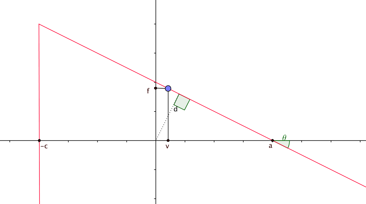
Figure 1: $B$ is the triangular region beneath the red line

Given the above reduction, we may now assume that $K$ is a wedge of the form
$\left\{(x,y)\in\mathbb{R}^{2}:x\geq-c,sx+ty\leq d\right\}$, $d,s,t\geq 0$, $s^{2}+t^{2}=1$, as in equation (24). We first take care of some trivial cases. Firstly, if $s=0,t=1$, we have $K=[-c,\infty)\times(-\infty,d]$. Then the height at $x=v$ is clearly $d$, and since $\gamma_{1}(-\infty,d)\geq\gamma_{2}(K)$, we get $d\geq g$ as is needed. Now assume that $s=1,t=0$, then $K=[-c,d]\times\mathbb{R}$, and hence the height at $x=v$ is infinite (note that $K$ always intersects the line at $x=v$ by the first part), and thus the desired bound trivially holds. We may thus assume that both $s,t>0$.

In this setting, the line $\ell=\left\{(x,y)\in\mathbb{R}^{2}:sx+ty=d\right\}$ intersects the x-axis at $a=d/s$ and forms an angle $\theta\in(0,\pi/2)$ with the x-axis as in Figure 1. Given the normalization $s^{2}+t^{2}=1$, note that $d$ is the perpendicular distance from $0$ to the edge $K\cap\ell$ of $K$. In what follows, we maintain the parametrization of the wedge $K$ in terms of $a$,$\theta$,$c$, using the relations $d=a\sin\theta$, $s=\sin\theta$ and $t=\cos\theta$ to recover $d,s,t$ when needed.

Recall that $\gamma_{2}(K)\geq\alpha=\gamma_{1}(-\infty,g)$ and $b(K)_{1}\geq 0$. Let $f^{*}=f(v,g)$ and let $f$ be the height of $K$ at $x=v$. We want to prove that $f\geq f^{*}$. If $f\geq g$, we are already done since $f^{*}\leq g$. Note that by Lemma 14, $f\geq g$ if $v=0$ and hence we may assume $v>0$. Our goal is now to show that $g-f\leq\min\left\{e^{\frac{g^{2}}{2}-\frac{1}{8ev^{2}}},(4e+2)\frac{v^{2}}{g}\right\}$.

Step 2: Using the barycenter condition

We now derive a bound on how large $d$ must be, given $c$ and $\theta$, such that the x-coordinate of barycenter is non-negative.

Let $H$ denote the halfspace $\left\{(x,y)\in\mathbb{R}^{2}:sx+ty\leq d\right\}$ and let $E=H\setminus K$. A simple computation shows $\int_{H}x\frac{1}{2\pi}e^{-1/2(x^{2}+y^{2})}{\rm dy\,dx}=-\frac{e^{-d^{2}/2}}{\sqrt{2\pi}}\sin\theta$. Now from the fact that $b(K)_{1}\geq 0$, and $E=H\setminus K$, we get

$$-\frac{e^{-d^{2}/2}}{\sqrt{2\pi}}\sin\theta\geq\int_{E}x\frac{1}{2\pi}e^{-1/2(x^{2}+y^{2})}{\rm dy\,dx}\geq\int_{x\leq-c}\frac{1}{\sqrt{2\pi}}xe^{-1/2x^{2}}{\rm dx}=-\frac{e^{-c^{2}/2}}{\sqrt{2\pi}}.$$ (27)

It follows that $\sin\theta\leq e^{-\frac{1}{2}(c^{2}-d^{2})}$. When $c^{2}\geq-2\log\sin\theta$, we get the following bound on $d$:

$$d\geq\sqrt{c^{2}+2\log\sin\theta}\text{ .}$$

When $c^{2}<-2\log\sin\theta$, this gives no useful bound on $d$ since in that case the barycenter is non-negative even for $d=0$. But $d\geq 0$ always as the Gaussian measure of $K$ is at least half. Thus,

$$d\geq\sqrt{\max\{0,c^{2}+2\log\sin\theta\}}\text{ .}$$ (28)

Step 3: Getting a bound on $f$

By construction of $K$, the point $(v,f)$ lies on the boundary of $H$, and hence

$$vs+ft=v\sin\theta+f\cos\theta=a\sin\theta=d\text{ .}$$ (29)

Now,

$$\frac{1}{\sqrt{2\pi}}\frac{e^{-\frac{1}{2}c^{2}}}{c+\sqrt{c^{2}+4}}\leq\frac{1}{2}\gamma_{1}(c,\infty)\leq\gamma_{2}(E)\qquad\textrm{(using lemma~{}\ref{lem:gaus-tail})}\text{ .}$$

Also,

$$\gamma_{2}(E)=\gamma_{2}(H)-\gamma_{2}(K)=\gamma_{1}(-\infty,d)-\gamma_{1}(-\infty,g)=\gamma_{1}(g,d)\leq\frac{1}{\sqrt{2\pi}}(d-g)e^{-\frac{1}{2}g^{2}}\qquad\textrm{(since $d\geq g\geq 0$)}\text{ .}$$

Combining the above two, we get

$$\frac{e^{\frac{1}{2}(g^{2}-c^{2})}}{c+\sqrt{c^{2}+4}}\leq d-g\text{ .}$$ (30)

From (28) and (30),

$$d\geq\max\{\sqrt{\max\{0,c^{2}+2\log\sin\theta\}},g+\frac{e^{\frac{1}{2}(g^{2}-c^{2})}}{c+\sqrt{c^{2}+4}}\}\text{ .}$$

Putting the above in (29),

$$f\geq\max\left\{\frac{\sqrt{\max\{0,c^{2}+2\log\sin\theta\}}-v\sin\theta}{\cos\theta},\frac{g+\frac{e^{\frac{1}{2}(g^{2}-c^{2})}}{c+\sqrt{c^{2}+4}}-v\sin\theta}{\cos\theta}\right\}\text{ .}$$

Observe that

$$\gamma_{1}(-\infty,g)=\gamma_{2}(K)\leq\gamma_{1}(-c,\infty)=\gamma_{1}(-\infty,c)\text{, }$$

giving $c\geq g$. Also $\theta\in[0,\pi/2]$. Thus, the above lower bound on $f$ holds if we minimize over all $c\geq g$ and $\theta\in[0,\pi/2]$.

$$f\geq\min_{c\geq g,\theta\in[0,\pi/2]}\max\left\{\frac{\sqrt{\max\{0,c^{2}+2\log\sin\theta\}}-v\sin\theta}{\cos\theta},\frac{g+\frac{e^{\frac{1}{2}(g^{2}-c^{2})}}{c+\sqrt{c^{2}+4}}-v\sin\theta}{\cos\theta}\right\}\text{ .}$$

We will first minimize with respect to $c$. For this, we make the following observations:

• for a fixed $\theta$, the first term inside the maximum is a non-decreasing function of $c$ while the second is a decreasing function of $c$.

• for $c=\sqrt{g^{2}-2\log\sin\theta}\geq g$, the first term is smaller than the second term

• for $c=\sqrt{g^{2}-2\log\sin\theta+1}\geq g$, the first term is greater than the second term.

Thus, the two terms must become equal somewhere in the range

$$c\in[\sqrt{g^{2}-2\log\sin\theta},\sqrt{g^{2}-2\log\sin\theta+1}]\text{ .}$$

In particular, substituting $c=\sqrt{g^{2}-2\log\sin\theta+1}$ in the second term provides a lower bound for $f$:

$$f \geq \min_{\theta\in[0,\pi/2]}\frac{g+\frac{\sin\theta}{\sqrt{e}(\sqrt{g^{2}-2\log\sin\theta+1}+\sqrt{g^{2}-2\log\sin\theta+5})}-v\sin\theta}{\cos\theta}$$

$$\geq \min_{\theta\in[0,\pi/2]}\frac{g+\frac{\sin\theta}{2\sqrt{e}\sqrt{g^{2}-2\log\sin\theta+5}}-v\sin\theta}{\cos\theta}\text{ .}$$

This expression goes to $g$ as $\theta\rightarrow 0$ and to $\infty$ as $\theta\rightarrow\pi/2$. If it is increasing in this whole interval, we are already done. Else, it achieves its minimum somewhere in $(0,\pi/2)$. Let this be at $\theta^{*}$. Setting the derivative to zero, we get

$$f \geq g\cos\theta^{*}-\frac{\sin 2\theta^{*}}{4\sqrt{e}\sqrt{g^{2}-2\log\sin\theta^{*}+5}^{3}}$$ (31)

$$= g-2g\sin^{2}(\theta^{*}/2)-\frac{\sin 2\theta^{*}}{4\sqrt{e}\sqrt{g^{2}-2\log\sin\theta^{*}+5}^{3}}\text{ ,}$$

where $\theta^{*}$ satisfies

$$v=g\sin\theta^{*}+\frac{1}{2\sqrt{e}\sqrt{g^{2}-2\log\sin\theta^{*}+5}}\text{ .}$$

From the two terms above, we can get two upper bounds on $\sin\theta^{*}$:

$$\sin\theta^{*} \leq v/g\text{ ,}$$

$$\sin\theta^{*} \leq \frac{e^{g^{2}/2+5/2}}{e^{\frac{1}{8ev^{2}}}}\text{ .}$$

Using these, we can simplify (31) as

$$f \geq g-2g\sin^{2}(\theta^{*}/2)-2e\sin 2\theta^{*}(v-g\sin\theta^{*})^{3}$$

$$\geq g-2g\sin^{2}(\theta^{*}/2)-2ev\sin 2\theta^{*}$$

$$\geq g-2g\sin^{2}(\theta^{*})-4ev\sin\theta^{*}\text{ .}$$

We derive two bounds on the above expression, one which will be useful when $g$ is small and other when $g$ is large. For the small $g$ bound, using that $v<v_{0}$ for $v_{0}$ small enough,

$$2g\sin^{2}(\theta^{*})+4ev\sin\theta^{*}\leq(2g\frac{v}{g}+4ev)\frac{e^{g^{2}/2+5/2}}{e^{\frac{1}{8ev^{2}}}}\leq\frac{e^{g^{2}/2}}{e^{\frac{1}{8ev^{2}}}}\text{ .}$$

For the large $g$ bound,

$$2g\sin^{2}(\theta^{*})+4ev\sin\theta^{*}\leq 2g\frac{v^{2}}{g^{2}}+\frac{4ev^{2}}{g}=(4e+2)\frac{v^{2}}{g}\text{ .}$$

Thus,

$$f\geq g-\min\{e^{\frac{g^{2}}{2}-\frac{1}{8ev^{2}}},(4e+2)\frac{v^{2}}{g}\}=f^{*}\text{ , as needed.}$$

∎

We now prove Theorem 41 in the special case where the barycenter lies to the right of the hyperplane $\theta^{\perp}$. We show later how to reduce Theorem 41 to this case.

Lemma 48.

There exists universal constants $v_{0},c_{0}>0$, such that for any $n\geq 1$, $v\in[0,v_{0}]$ and $\theta\in\mathbb{R}^{n}$, $\|\theta\|_{2}=1$, convex body $K\subseteq\mathbb{R}^{n}$ satisfying $\gamma_{n}(K)=\alpha\geq 1/2$ and $\langle{b(K),\theta}\rangle\geq 0$, we have that

$$\gamma_{n-1}(K_{v}^{\theta})\geq\alpha(1-\frac{e^{-\frac{1}{100v^{2}}}}{4\sqrt{2\pi}})\text{.}$$

Proof.

We split the proof into two steps. In step one, we reduce to a 2-dimensional problem and show that it suffices to prove our theorem for a downwards closed convex body $K^{\prime}\subseteq\mathbb{R}^{2}$. This reduction will guaranteee that $K^{\prime}$ has barycenter on the y-axis and that the Gaussian measure of slices of $K^{\prime}$ parallel to the y-axis will correspond in the natural way to that of slices of $K$ parallel to the hyperplane $\theta^{\perp}=\left\{x\in\mathbb{R}^{n}:\langle{x,\theta}\rangle=0\right\}$. We then invoke Lemma 47 to get a lower bound on the height of $K^{\prime}$ at $x=v$. Lastly, in step 2, we show that implies the required lower bound on the slice measure.

Let $g$ be s.t. $\gamma_{1}(-\infty,g)=\alpha$, i.e. $g=\Phi^{-1}(\alpha)$. Note that $g\geq 0$ since $\alpha\geq 1/2$.

Step 1: reduction to a 2-dimensional case

We will reduce our problem to one for a $2$-dimensional downwards closed convex body $K^{\prime}$. To specify $K^{\prime}$, we need only specify the height of the boundary at each x-coordinate. At x-coordinate $t$, we define the height of $K^{\prime}$ to be the $y_{t}$ satisfying $\gamma_{1}(-\infty,y_{t})=\gamma_{n-1}(K^{\theta}_{t})$. From Ehrhard’s inequality, we see that $K^{\prime}$ is in fact convex. Furthermore, it is easy to check that $\gamma_{2}(K^{\prime})=\gamma_{n}(K)$ and $b(K^{\prime})_{1}=\langle{b(K),\theta}\rangle\geq 0$.

Thus, $K^{\prime}$ is a downwards closed convex body in $\mathbb{R}^{2}$ with $\gamma_{2}(K^{\prime})=\alpha,b(K^{\prime})_{1}\geq 0$. From here, we may invoke Lemma 47 to conclude that the height of $K^{\prime}$ at $x=v$ is at least $f^{*}:=f(v,g)$. We now have that

$$\gamma_{n-1}(K^{\theta}_{t})=\gamma_{1}(-\infty,y_{t})\geq\gamma_{1}(-\infty,f^{*})\text{ .}$$

From the above, it suffices to give a lower bound on $\gamma_{1}(-\infty,f^{*})$ in order to derive the theorem.

Step 2: Bounding $\gamma_{1}(-\infty,f^{*})$

Our goal is to show that $\gamma_{1}(-\infty,f^{*})\geq\alpha(1-\frac{e^{-\frac{1}{100v^{2}}}}{4\sqrt{2\pi}})$. Clearly, it suffices to show $\gamma_{1}(f^{*},g)\leq\alpha\frac{e^{-\frac{1}{100v^{2}}}}{4\sqrt{2\pi}}$. Let $\varepsilon_{g}=g-f^{*}=\min\left\{e^{\frac{g^{2}}{2}-\frac{1}{8ev^{2}}},(4e+2)\frac{v^{2}}{g}\right\}$. We split the analysis in two cases depending on whether $g$ is small or big.

Step 2a: $g\leq\frac{1}{5v}$

$$\gamma_{1}(f^{*},g)\leq\frac{\varepsilon_{g}}{\sqrt{2\pi}}\leq\frac{e^{\frac{g^{2}}{2}-\frac{1}{8ev^{2}}}}{\sqrt{2\pi}}\leq\frac{e^{\frac{1}{50v^{2}}-\frac{1}{8ev^{2}}}}{\sqrt{2\pi}}\leq\frac{e^{-\frac{1}{100v^{2}}}}{8\sqrt{2\pi}}\leq\alpha\frac{e^{-\frac{1}{100v^{2}}}}{4\sqrt{2\pi}}\text{ .}$$

The penultimate inequality holds for an appropriate choice of $v_{0}$, and the last inequality uses $\alpha\geq 1/2$.

Step 2b: $g>\frac{1}{5v}$

Here we will use the other bound for $\varepsilon_{g}$.

$$\gamma_{1}(f^{*},g) \leq \frac{\varepsilon_{g}}{\sqrt{2\pi}}e^{-(f^{*})^{2}/2}=\frac{\varepsilon_{g}}{\sqrt{2\pi}}e^{-g^{2}/2}e^{g\varepsilon_{g}-\varepsilon_{g}^{2}/2}$$

$$\leq \frac{\varepsilon_{g}}{\sqrt{2\pi}}e^{-g^{2}/2+g\varepsilon_{g}}\leq\frac{(4e+2)v^{2}}{g\sqrt{2\pi}}e^{-g^{2}/2+(4e+2)v^{2}}$$

$$\leq \frac{5(4e+2)v^{3}}{\sqrt{2\pi}}e^{-\frac{1}{50v^{2}}+(4e+2)v^{2}}\leq\frac{e^{-\frac{1}{100v^{2}}}}{8\sqrt{2\pi}}\leq\alpha\frac{e^{-\frac{1}{100v^{2}}}}{4\sqrt{2\pi}}\text{ .}$$

The penultimate inequality holds for an appropriate choice of $v_{0}$, and the last inequality uses $\alpha\geq 1/2$. ∎

We now come to the proof of Theorem 41.

Theorem 41 (restated): There exist universal constants $v_{0},\eta_{0},c_{0}>0$, such that for any $n\geq 1$, convex body $K\subseteq\mathbb{R}^{n}$ satisfying $\|b(K)\|_{2}=\eta\leq\eta_{0}$ and $\gamma_{n}(K)=\alpha\geq 3/5$, $v\in[-v_{0},v_{0}]$ and $\theta\in\mathbb{R}^{n}$, $\|\theta\|_{2}=1$, we have that

$$\gamma_{n-1}(K_{v}^{\theta})\geq(\alpha-c_{0}\eta)(1-\frac{e^{-\frac{1}{100v^{2}}}}{4\sqrt{2\pi}})\text{.}$$

Proof.

By rotational invariance, we may assume that $\theta=e_{1}$, the first standard basis vector. By possibly replacing $K$ by $-K$, we may also assume that $v\geq 0$.

If $b(K)_{1}\geq 0$, the desired lower bound follows directly from Lemma 48. Given this, we may assume that $-\eta\leq b(K)_{1}<0$. To deal with this second case, the main idea is to remove some portion of $K$ lying to the left of the hyperplane $e_{1}^{\perp}=\left\{x\in\mathbb{R}^{n}:x_{1}=0\right\}$ so that the barycenter of the remaining body lies on $e_{1}^{\perp}$. After this, we apply Lemma 48 again on the truncated body.

Define

$$b:=b(K)_{1}\gamma_{n}(K)=\int_{K}x_{1}\frac{e^{-\frac{1}{2}\|x\|^{2}_{2}}}{\sqrt{2\pi}^{n}}{\rm dx}<0\text{ .}$$

Let $H^{-}_{t}=\left\{x\in\mathbb{R}^{n}:x_{1}\leq t\right\}$ and $H^{+}_{t}=\left\{x\in\mathbb{R}^{n}:x_{1}\geq t\right\}$ for $t\in\mathbb{R}$. Let $z<0$ be defined as the smallest negative number satisfying

$$\int_{K\cap H^{+}_{z}}x_{1}\frac{e^{-\frac{1}{2}\|x\|_{2}^{2}}}{\sqrt{2\pi}^{n}}{\rm dx}=0\text{ .}$$ (32)

By continuity, such a $z$ must exists, since as $z\rightarrow-\infty$ the left hand side tends to $b<0$ and at $z=0$ it is positive. Given the above, note that $b(K\cap H^{+}_{z})_{1}=0$. We will now show that $\gamma_{n}(K\cap H^{+}_{z})\geq\alpha-c_{0}\eta$ if $\eta\leq\eta_{0}$, for $c_{0},\eta_{0}$ appropriately chosen constants.

By our choice of $z$, we have the equality

$$\int_{K\cap H^{-}_{z}}x_{1}\frac{e^{-\frac{1}{2}\|x\|_{2}^{2}}}{\sqrt{2\pi}^{n}}{\rm dx}=b\text{ .}$$

From here, we see that

$$\gamma_{n}(K\cap H^{-}_{z})=\int_{K\cap H^{-}_{z}}\frac{e^{-\frac{1}{2}\|x\|^{2}_{2}}}{\sqrt{2\pi}^{n}}{\rm dx}\leq\int_{K\cap H^{-}_{z}}\frac{x_{1}}{z}\frac{e^{-\frac{1}{2}\|x\|^{2}_{2}}}{\sqrt{2\pi}^{n}}{\rm dx}=\frac{b}{z}=\left|\frac{b}{z}\right|\text{ .}$$

Given this, we get that

$$\gamma_{n}(K\cap H^{+}_{z})=\gamma_{n}(K)-\gamma_{n}(K\cap H^{-}_{z})=\alpha-\gamma_{n}(K\cap H^{-}_{z})\geq\alpha-\left|\frac{b}{z}\right|\geq\alpha-\left|\frac{\eta}{z}\right|\text{ .}$$

We now show that there exists a constant $c_{0}$ s.t. $1/|z|\leq c_{0}$. Let $\beta=\gamma_{n}(K\cap H^{+}_{0})$, and note that

$$\beta=\gamma_{n}(K)-\gamma_{n}(K\cap H^{-}_{0})\geq\alpha-1/2\geq 3/5-1/2=1/10\text{ .}$$

Let $\tau>0$ be positive number satisfying $\gamma_{1}(0,\tau)=\beta$, i.e. $\tau=\Phi^{-1}(1/2+\beta)$. By pushing the mass of $K\cap H^{+}_{0}$ to the left towards $e_{1}^{\perp}$ as much as possible, we see that

$$\int_{K\cap H^{+}_{0}}x_{1}\frac{e^{-\frac{1}{2}\|x\|_{2}^{2}}}{\sqrt{2\pi}^{n}}{\rm dx}\geq\int_{\left\{x\in\mathbb{R}^{n}:0\leq x_{1}\leq\tau\right\}}x_{1}\frac{e^{-\frac{1}{2}\|x\|_{2}^{2}}}{\sqrt{2\pi}^{n}}{\rm dx}=\frac{1}{\sqrt{2\pi}}(1-e^{-\tau^{2}/2})\text{ .}$$ (33)

Next, by inclusion

$$\int_{K\cap\left\{x\in\mathbb{R}^{n}:z\leq x\leq 0\right\}}x_{1}\frac{e^{-\frac{1}{2}\|x\|_{2}^{2}}}{\sqrt{2\pi}^{n}}{\rm dx}\geq\int_{\left\{x\in\mathbb{R}^{n}:z\leq x\leq 0\right\}}x_{1}\frac{e^{-\frac{1}{2}\|x\|_{2}^{2}}}{\sqrt{2\pi}^{n}}{\rm dx}=\frac{1}{\sqrt{2\pi}}(e^{-z^{2}/2}-1)\text{ .}$$ (34)

Given that $z$ satisfies (32), combining equations (33), (34), we must have that

$$0\geq e^{-z^{2}/2}-e^{-\tau^{2}/2}\Rightarrow|z|\geq\tau\geq\Phi^{-1}(6/10)>0\text{ .}$$

Thus, we may set $c_{0}=1/\Phi^{-1}(6/10)$. Set $\eta_{0}=\frac{1}{10c_{0}}$. Since $\eta\leq\eta_{0}$, we have that

$$\gamma_{n}(K\cap H^{+}_{z})\geq\alpha-c_{0}\eta\geq 3/5-1/10=1/2\text{ .}$$

Lastly, using Lemma 48 on $K\cap H^{+}_{z}$, we now get that

$$\gamma_{n-1}(K^{e_{1}}_{v})=\gamma_{n-1}((K\cap H^{+}_{z})^{e_{1}}_{v})\geq(\alpha-c_{0}\eta)(1-\frac{e^{-\frac{1}{100v^{2}}}}{4\sqrt{2\pi}})\text{ ,}$$

as needed. ∎

10 Constructive Vector Komlós

In this section we give a new proof of the main result of [24] that the natural SDP for the Komlós problem has value at most $1$. While the proof in [24] used duality, our proof is direct and immediately yields an algorithm to compute an SDP solution which only uses basic linear algebraic operations, and does not need a general SDP solver. We state the main theorem next.

Theorem 49.

Let $v_{1},\ldots,v_{n}\in\mathbb{R}^{m}$ be vectors of Euclidean length at most $1$, and let $\alpha_{1},\ldots,\alpha_{n}\in[0,1]$. There exists an $n\times n$ PSD matrix $X$ such that

$$X_{ii} =\alpha_{i}\ \ \ \forall 1\leq i\leq n$$

$$VXV^{\mathsf{T}} \preceq I_{m},$$

where $V=(v_{1},\ldots,v_{m})$ is the $n\times m$ matrix whose columns are the vectors $v_{i}$.

To prove Theorem 49 we make use of a basic identity about inverses of block matrices. This is a standard use of the Schur complement and we will not prove it here.

Lemma 50.

Let

$$A=\left(\begin{array}[]{cc}A_{11}&A_{12}\\ A_{21}&A_{22}\\ \end{array}\right)$$

be a $(k+\ell)\times(k+\ell)$ block matrix, where $A_{11}$ is a $k\times k$ matrix, $A_{12}$ is a $k\times\ell$ matrix, $A_{21}$ is a $\ell\times k$ matrix, and $A_{22}$ is a $\ell\times\ell$ matrix. Assume $A$ and $A_{22}$ are invertible, and write $B=A^{-1}$ in block form as

$$B=\left(\begin{array}[]{cc}B_{11}&B_{12}\\ B_{21}&B_{22}\\ \end{array}\right),$$

where $B_{ij}$ has the same dimensions as $A_{ij}$. Then $B_{11}=(A_{11}-A_{12}A_{22}^{-1}A_{21})^{-1}$ (i.e. the inverse of the Schur complement of $A_{11}$ in $A$).

From Lemma 50 we derive the main technical claim used in the proof of Theorem 49.

Lemma 51.

Let $A=V^{\mathsf{T}}V$ be an $n\times n$ positive definite matrix, and let $v_{1},\ldots,v_{n}$ be the columns of $V$. Let $B=A^{-1}$. Then, for each $1\leq i\leq n$

$$B_{ii}=\frac{1}{\|(I-\Pi_{-i})v_{i}\|_{2}^{2}}\geq\frac{1}{\|v_{i}\|_{2}^{2}},$$

where $\Pi_{-i}$ is the orthogonal projection matrix onto $\mathrm{span}\{v_{j}:j\neq i\}$.

Proof.

It is sufficient to prove the lemma for $i=1$. Let $U$ be the matrix with columns $v_{2},\ldots,v_{n}$. Since $A$ is positive definite, the principal minor $U^{\mathsf{T}}U$ is positive definite as well, and, therefore, invertible. By Lemma 50,

$$B_{11}=\frac{1}{\|v_{1}\|_{2}^{2}-v_{1}^{\mathsf{T}}U(U^{\mathsf{T}}U)^{-1}U^{\mathsf{T}}v_{1}}.$$

Let $\Pi=U(U^{\mathsf{T}}U)^{-1}U^{\mathsf{T}}$. Since $\Pi$ is symmetric and idempotent (i.e. $\Pi^{2}=\Pi$), it is an orthogonal projection matrix. Moreover $\Pi U=U$ and $\Pi$ has the same rank as $U$, so $\Pi$ is the orthogonal projection matrix onto the column span of $U$, i.e. $U(U^{\mathsf{T}}U)^{-1}U^{\mathsf{T}}=\Pi_{-1}$ and the lemma follows. ∎

Proof of Theorem 49.

We prove the theorem by induction on $n$.

In the base case $m=1$, we have a single vector $v\in\mathbb{R}^{m}$, $\|v\|_{2}\leq 1$, and an $\alpha\in[0,1]$. We set $x=\alpha$, and we clearly have $vxv^{T}\preceq\alpha I\preceq I$.

We now proceed with the inductive step. Consider first the case that $V^{\mathsf{T}}V$ is singular. Then there exists a vector $x\neq 0$ such that $Vx=0$. Scale $x$ so that $x_{i}^{2}\leq\alpha_{i}$ for all $i$, and there exists $k$ such that $x_{k}^{2}=\alpha_{k}^{2}$. Apply the inductive hypothesis to the vectors $(v_{i}:i\neq k)$ and the reals $(\alpha^{\prime}_{i}=\alpha_{i}-x_{i}^{2}:i\neq k)$ to get a matrix $Y\in\mathbb{R}^{([m]\setminus\{k\})\times([n]\setminus\{k\})}$. Extend $Y$ to a matrix $\tilde{Y}\in\mathbb{R}^{n\times n}$ by padding with $0$’s, i.e. $\tilde{Y}_{ij}=Y_{ij}$ if $i,j\neq k$ and $\tilde{Y}_{ij}=0$, otherwise. Define $X=xx^{\mathsf{T}}+\tilde{Y}$: it is easy to verify that both conditions of the theorem are satisfied.

Finally, assume that $V^{\mathsf{T}}V$ is invertible, and let $B=(V^{\mathsf{T}}V)^{-1}$. Define

$$\beta =\min_{i}\alpha_{i}/B_{ii},$$

$$k =\arg\min_{i}\alpha_{i}/B_{ii},$$

$$\gamma =\max_{i}\alpha_{i}-\beta B_{ii}.$$

Apply the inductive hypothesis to the vectors $(v_{i}:i\neq k)$ and the reals $(\alpha^{\prime}_{i}=(\alpha_{i}-\beta b_{ii})/\gamma:i\neq k)$ to get a matrix $Y\in\mathbb{R}^{([n]\setminus\{k\})\times([n]\setminus\{k\})}$, which we then pad with $0$’s to an $n\times n$ matrix $\tilde{Y}$, as we did in the first case above. Define $X$ as $X=\beta B+\gamma\tilde{Y}$. It is easy to verify that $X_{ii}=\alpha_{i}$ for all $i$. We have

$$VXV^{\mathsf{T}}=\beta VBV^{\mathsf{T}}+\gamma V^{\mathsf{T}}\tilde{Y}V=\beta V(V^{\mathsf{T}}V)^{-1}V^{\mathsf{T}}+\gamma U^{\mathsf{T}}YU,$$

where $U$ is the submatrix of $V$ consisting of all columns of $V$ except $v_{k}$. $U^{\mathsf{T}}YU\preceq I$ by the induction hypothesis. Since $V(V^{\mathsf{T}}V)^{-1}V^{\mathsf{T}}$ is symmetric and idempotent, it is an orthogonal projection matrix, and therefore $V(V^{\mathsf{T}}V)^{-1}V^{\mathsf{T}}\preceq I$. Because $B_{ii}\geq\|v_{i}\|_{2}^{-2}\geq 1$ by Lemma 51, we have $\gamma\leq\max_{i}\alpha_{i}-\beta$. Therefore,

$$VXV^{\mathsf{T}}=\beta V(V^{\mathsf{T}}V)^{-1}V^{\mathsf{T}}+\gamma U^{\mathsf{T}}YU\preceq(\beta+\gamma)I_{n}\preceq(\max_{i}\alpha_{i})I_{n}\preceq I_{n}.$$

This completes the proof. ∎

Observe that the proof of Theorem 49 can be easily turned into an efficient recursive algorithm.

11 Appendix

11.1 Estimating the Barycenter

In this section we show how to efficiently estimate the barycenter of $K$ up to a small accuracy in $\ell_{2}$-norm. For a convex body $K\subseteq\mathbb{R}^{n}$, we let $\gamma_{K}$ denote the Gaussian measure restricted to $K$. For a random variable $X$ in $\mathbb{R}^{n}$, we denote the covariance of $X$ by $cov[X]=\operatorname*{\mathbb{E}}[(X-\operatorname*{\mathbb{E}}[X])(X-\operatorname*{\mathbb{E}}[X])^{\mathsf{T}}]$.

The following lemma shows that the covariance of a Gaussian random vector shrinks when restricted to a convex body. We include a short proof for completeness.

Lemma 52.

Given a convex body $K$ in $\mathbb{R}^{n}$, let $\gamma_{K}$ be the Gaussian distribution restricted to $K$, and let $X$ be a random variable distributed according to $\gamma_{K}$. Then, $cov[X]\preceq I_{n}$.

Proof.

Consider $f(t)=\ln\,\gamma_{n}(K+t)$. $f$ is concave in $t$. This follows from log-concavity of $\gamma_{n}$, an easy consequence of the Prekopa-Leindler inequality. Hence, the Hessian of $f$, $H(f)$, is negative semi-definite. It can be calculated that

$$H(f)=H(\ln\,\gamma_{n}(K+t))=cov[X+t]-I_{n},$$

where $X\sim\gamma_{K}$. Setting $t=0$ completes the proof. ∎

We will also need to use Paouris’ inequality [26], which we restate slightly:

Theorem 53.

If $X\subseteq\mathbb{R}^{n}$ is a log-concave random vector with mean $0$ and positive-definite covariance matrix $C$, then for every $t\geq 1$,

$$\Pr[\sqrt{X^{\mathsf{T}}C^{-1}X}\geq\beta t\sqrt{n}]\leq e^{-t\sqrt{n}}$$

where $\beta>0$ is an absolute constant.

Theorem 54.

Let $K$ be a convex body in $\mathbb{R}^{n}$, given by a membership oracle, with $\gamma_{n}(K)\geq 1/2$. For any $\delta>0$ and $\varepsilon\in(0,1)$, there is an algorithm which computes the barycenter of $K$ within accuracy $\delta$ in $\ell_{2}$-norm with probability at least $1-\varepsilon$ in time polynomial in $n,1/\delta$ and $\log(1/\varepsilon)$.

Proof.

Let $b$ be the barycenter of $K$ and $X_{i}$ for $1\leq i\leq N$ be i.i.d generated from $\gamma_{K}$, where $N=\lceil(\beta/\delta)^{2}\log^{2}(e/\varepsilon)n\rceil$. Here $\beta$ is the constant from Theorem 53. Defining the following quantities

$$b^{\prime} = \frac{1}{N}\sum_{i=1}^{N}X_{i}$$

$$Y_{i} = X_{i}-b$$

$$Y = \frac{1}{N}\sum_{i=1}^{N}Y_{i}$$

$$C = \operatorname*{\mathbb{E}}_{X\sim\gamma_{K}}[(X-b)(X-b)^{\mathsf{T}}]$$

we can see that $b^{\prime}$ is an estimate of the barycenter, generated by averaging random samples from the distribution $\gamma_{K}$ and $Y$ is the difference vector between the true barycenter and $b^{\prime}$. Thus it suffices to bound the probability that $Y$ is large and then show how to efficiently generate random samples from the distribution $\gamma_{K}$. It holds that

$$\operatorname*{\mathbb{E}}[Y_{i}]=\operatorname*{\mathbb{E}}[X_{i}-b]=b-b=0$$

Also, using Lemma 52,

$$\operatorname*{\mathbb{E}}[Y_{i}Y_{i}^{\mathsf{T}}]=cov[X_{i}]=C\preceq I_{n}$$

Thus,

$$\operatorname*{\mathbb{E}}[Y]=0\textrm{ and }cov[Y]=C/N\preceq I_{n}/N$$

Since $\gamma_{K}$ is a log-concave distribution, $X_{i}$ and hence $Y_{i}$ are log-concave random vectors. It is easily checked (using the Prekopa-Leindler inequality) that the average of log-concave random variables is also log-concave and hence $Y$ is a log-concave random vector. Now,

$$\Pr[\|Y\|_{2}\geq\delta] = \Pr\left[\sqrt{Y^{\mathsf{T}}\left(\frac{I_{n}}{N}\right)^{-1}Y}\geq\delta\sqrt{N}\right]$$

$$\leq \Pr\left[\sqrt{Y^{\mathsf{T}}\left(\frac{C}{N}\right)^{-1}Y}\geq\delta\sqrt{N}\right]\qquad\textrm{(using $C/N\preceq I_{n}/N$)}$$

Putting $N=\lceil(\beta/\delta)^{2}\log^{2}(e/\varepsilon)n\rceil$ and using Theorem 53 with $t=\log(e/\varepsilon)$, we get

$$\Pr[\|Y\|_{2}\geq\delta]\leq e^{-\sqrt{n}\log(e/\varepsilon)}\leq\varepsilon/e\leq\varepsilon/2.$$ (35)

We can generate the random points $X_{i}$ using rejection sampling. For each $i$, we generate a sequence of i.i.d. standard Gaussian random variables $X_{i}^{(1)},\ldots,X_{i}^{(k)}\in\mathbb{R}^{n}$, $k=\lceil\log_{2}(2N/\varepsilon)\rceil$. We set $X_{i}$ to the first $X_{i}^{(j)}$ in the sequence that belongs to $K$; if no such $X_{i}^{(j)}$ exists, we set $X_{i}$ arbitrarily. Clearly, conditional on the existence of a $j\leq k$ such that $X_{i}^{(j)}\in K$, $X_{i}\sim\gamma_{K}$. Furthermore, because $K$ has Gaussian measure at least $1/2$, for every $j$ we have $\Pr[X_{i}^{(j)}\not\in K]\leq 1/2$, so

$$\Pr[\forall j:X_{i}^{(j)}\not\in K]\leq 2^{-k}\leq\varepsilon/2N.$$

By a union bound, with probability at least $1-\varepsilon/2$, all $X_{i}$ are distributed according to $\gamma_{K}$; let us call this event $E$. Conditional on $E$, inequality (35) holds, and

$$\Pr[\|b-b^{\prime}\|_{2}\geq\delta] =\Pr[\|Y\|_{2}\geq\delta]$$

$$=\Pr[\|Y\|_{2}\geq\delta\mid E]\cdot\Pr[E]+\Pr[\|Y\|_{2}\geq\delta\mid E^{c}](1-\Pr[E])$$

$$\leq\varepsilon/2+\varepsilon/2=\varepsilon.$$

The algorithm needs to generate $O(N\log(N/\varepsilon))$ $d$-dimensional Gaussian random variables, check membership in $K$ for each of them, and compute the average of $N$ points. Since each of these operations takes polynomial time, and $N$ is polynomial in $n$, $\delta$, and $\log(1/\varepsilon)$, the running time of the algorithm is polynomial.

∎

11.2 Proof of Lemma 11

Proof.

We first prove subgaussianity. Let $\theta\in S^{n-1}$, $t\geq 0$. By assumption on $X$,

$$\Pr[|\langle{X,\theta}\rangle|\geq t] =\min_{\lambda>0}\Pr[\cosh(\lambda\langle{X,\theta}\rangle)\geq\cosh(\lambda t)]\leq\min_{\lambda>0}\beta\cdot\frac{e^{\sigma^{2}\lambda^{2}/2}}{\cosh(\lambda t)}$$

$$\leq\min_{\lambda>0}2\beta\cdot e^{\sigma^{2}\lambda^{2}/2-\lambda t}\leq 2\beta\cdot e^{-\frac{1}{2}(t/\sigma)^{2}}\text{, }$$

where the last inequality follows by setting $\lambda=t/\sigma^{2}$.

Let $\alpha=\sqrt{\log_{2}\beta+1}$. To prove that $X$ is $\alpha\sigma$-subgaussian, since probabilities are always at most one, it suffices to prove that

$$\min\left\{1,2\beta\cdot e^{-\frac{1}{2}(t/\sigma)^{2}}\right\}\leq 2e^{-\frac{1}{2}(t/(\alpha\sigma))^{2}},\forall t\geq 0\text{.}$$

Replacing $t\leftarrow\sqrt{2}\sigma t$, the above simplifies to showing

$$\min\left\{1,2\beta\cdot e^{-t^{2}}\right\}\leq 2e^{-(t/\alpha)^{2}},\forall t\geq 0\text{.}$$ (36)

From here, we see that

$$\beta\cdot e^{-t^{2}}\leq e^{-(t/\alpha)^{2}}\Leftrightarrow\beta\leq e^{(1-1/\alpha^{2})t^{2}}\Leftrightarrow t\geq\sqrt{\ln\beta\cdot\frac{\alpha^{2}}{\alpha^{2}-1}}=\sqrt{\ln(2\beta)}\text{.}$$ (37)

Let $r=\sqrt{\ln(2\beta)}$, noting that $1=2\beta\cdot e^{-r^{2}}=2e^{-(r/\alpha)^{2}}$, we have that for $t\leq r$, the LHS of 36 is $1$ and the RHS is at least $1$, for $t>r$, the LHS is equal to $2\beta\cdot e^{-t^{2}}$ and the RHS is larger by 37. Thus, $X$ is $\alpha\sigma$-subgaussian as needed.

We now prove the furthermore. For $X$ an $n$-dimensional standard Gaussian, note that $\langle{X,w}\rangle$ is distributed like $\sigma Y$, where $Y\sim N(0,1)$ and $\sigma=\|\mathbf{w}\|_{2}$. Hence,

$$\operatorname*{\mathbb{E}}[e^{\langle{X,w}\rangle}] =\operatorname*{\mathbb{E}}[e^{\sigma Y}]=\frac{1}{\sqrt{2\pi}}\int_{-\infty}^{\infty}e^{\sigma x}e^{-x^{2}/2}dx$$

$$=e^{\sigma^{2}/2}\left(\frac{1}{\sqrt{2\pi}}\int_{-\infty}^{\infty}e^{-(x-\sigma)^{2}/2}dx\right)=e^{\sigma^{2}/2}\text{, }$$

as needed. ∎

References

- [1] Milton Abramowitz and Irene A. Stegun, editors. Handbook of mathematical functions with formulas, graphs, and mathematical tables. Dover Publications, Inc., New York, 1992. Reprint of the 1972 edition.
- [2] Wojciech Banaszczyk. Balancing vectors and Gaussian measures of -dimensional convex bodies. Random Structures Algorithms, 12(4):351–360, 1998.
- [3] Wojciech Banaszczyk. On series of signed vectors and their rearrangements. Random Struct. Algorithms, 40(3):301–316, 2012. URL: http://dx.doi.org/10.1002/rsa.20373, doi:10.1002/rsa.20373.
- [4] Nikhil Bansal. Constructive algorithms for discrepancy minimization. In 2010 IEEE 51st Annual Symposium on Foundations of Computer Science FOCS 2010, pages 3–10. IEEE Computer Soc., Los Alamitos, CA, 2010.
- [5] Nikhil Bansal, Daniel Dadush, and Shashwat Garg. An algorithm for Komlós conjecture matching Banaszczyk’s bound. In 57th Annual IEEE Symposium on Foundations of Computer Science, FOCS 2016, New Brunswick, NJ, USA, October 9-11, 2016, pages 788–799, 2016.
- [6] Franck Barthe, Olivier Guédon, Shahar Mendelson, and Assaf Naor. A probabilistic approach to the geometry of the -ball. Ann. Probab., 33(2):480–513, 2005.
- [7] József Beck. Roth’s estimate of the discrepancy of integer sequences is nearly sharp. Combinatorica, 1(4):319–325, 1981.
- [8] József Beck and Tibor Fiala. “Integer-making” theorems. Discrete Appl. Math., 3(1):1–8, 1981.
- [9] Christer Borell. The Ehrhard inequality. C. R. Math. Acad. Sci. Paris, 337(10):663–666, 2003.
- [10] Boris Bukh. An improvement of the Beck-Fiala theorem. CoRR, abs/1306.6081, 2013.
- [11] Bernard Chazelle. The discrepancy method. Cambridge University Press, Cambridge, 2000. Randomness and complexity.
- [12] William Chen, Anand Srivastav, Giancarlo Travaglini, et al. A Panorama of Discrepancy Theory, volume 2107. Springer, 2014.
- [13] Antoine Ehrhard. Symétrisation dans l’espace de Gauss. Math. Scand., 53(2):281–301, 1983.
- [14] Ronen Eldan and Mohit Singh. Efficient algorithms for discrepancy minimization in convex sets. CoRR, abs/1409.2913, 2014.
- [15] Esther Ezra and Shachar Lovett. On the Beck-Fiala conjecture for random set systems. Electronic Colloquium on Computational Complexity (ECCC), 22:190, 2015.
- [16] David A. Freedman. On tail probabilities for martingales. Ann. Probability, 3:100–118, 1975.
- [17] Nicholas J. A. Harvey, Roy Schwartz, and Mohit Singh. Discrepancy without partial colorings. In Approximation, randomization, and combinatorial optimization, volume 28 of LIPIcs. Leibniz Int. Proc. Inform., pages 258–273. Schloss Dagstuhl. Leibniz-Zent. Inform., Wadern, 2014.
- [18] Rafał Latała and Krzysztof Oleszkiewicz. Gaussian measures of dilatations of convex symmetric sets. Ann. Probab., 27(4):1922–1938, 1999.
- [19] Avi Levy, Harishchandra Ramadas, and Thomas Rothvoss. Deterministic discrepancy minimization via the multiplicative weight update method. arXiv preprint arXiv:1611.08752, 2016.
- [20] L. Lovász, J. Spencer, and K. Vesztergombi. Discrepancy of set-systems and matrices. European J. Combin., 7(2):151–160, 1986. URL: http://dx.doi.org/10.1016/S0195-6698(86)80041-5, doi:10.1016/S0195-6698(86)80041-5.
- [21] Shachar Lovett and Raghu Meka. Constructive discrepancy minimization by walking on the edges. SIAM J. Comput., 44(5):1573–1582, 2015. Preliminary version in FOCS 2012.
- [22] Jiří Matoušek. Geometric discrepancy, volume 18 of Algorithms and Combinatorics. Springer-Verlag, Berlin, 1999. An illustrated guide.
- [23] John Von Neumann. Zur theorie der gesellschaftsspiele. Mathematische Annalen, 100(1):295–320, 1928.
- [24] Aleksandar Nikolov. The Komlós conjecture holds for vector colorings. arXiv preprint arXiv:1301.4039, 2013.
- [25] Aleksandar Nikolov and Kunal Talwar. Approximating hereditary discrepancy via small width ellipsoids. In Symposium on Discrete Algorithms, SODA, pages 324–336, 2015.
- [26] G. Paouris. Concentration of mass on convex bodies. Geom. Funct. Anal., 16(5):1021–1049, 2006.
- [27] Thomas Rothvoss. Constructive discrepancy minimization for convex sets. In 55th Annual IEEE Symposium on Foundations of Computer Science—FOCS 2014, pages 140–145. IEEE Computer Soc., Los Alamitos, CA, 2014.
- [28] Joel Spencer. Six standard deviations suffice. Trans. Amer. Math. Soc., 289(2):679–706, 1985.
- [29] Joel Spencer. Ten lectures on the probabilistic method, volume 52. SIAM, 1987.
- [30] Aravind Srinivasan. Improving the discrepancy bound for sparse matrices: better approximations for sparse lattice approximation problems. In Proceedings of the Eighth Annual ACM-SIAM Symposium on Discrete Algorithms (New Orleans, LA, 1997), pages 692–701. ACM, New York, 1997.
- [31] Michel Talagrand. The generic chaining. Springer Monographs in Mathematics. Springer-Verlag, Berlin, 2005. Upper and lower bounds of stochastic processes.