TTK-16-48

Resonance-improved parton-shower matching
for the Drell–Yan process including
electroweak corrections

A. Mück and L. Oymanns

Institut für Theoretische Teilchenphysik und Kosmologie,

RWTH Aachen University,

D-52056 Aachen, Germany

We use the Powheg method to perform parton-shower matching for Drell–Yan production of W and Z bosons at the LHC at NLO QCD and NLO electroweak accuracy. In particular, we investigate an improved treatment of the vector-boson resonances within the Powheg method. We employ an independent implementation of the Powheg method and compare to earlier results within the Powheg-Box. On the technical side, we provide the FKS formalism for photon-radiation off fermions within mass regularization.

1 Introduction

The Drell–Yan process is a standard-candle process at the CERN Large Hadron Collider (LHC). Due to the high statistics for the production of W and Z bosons and the clean signature of their leptonic decays, it allows for precision measurements and a thorough test of our theoretical understanding of hadron-collider physics (see e.g. Refs. [1, 2] for recent reviews). For example, the Drell–Yan process at the LHC is used to measure the W-boson mass [3] with unprecedented accuracy and Z-boson production is sensitive to the effective weak mixing angle. Moreover, the Drell–Yan process is an excellent tool to extract information on the partonic content of the proton and is employed in PDF fits. Concerning new physics, Drell–Yan production is an important background for Z’ or W’ searches. For many other searches, the modeling of weak-boson production at large transverse momentum is essential.

To match the experimental precision, the theory predictions have been improved and refined continuously. Due to its simplicity, the Drell–Yan process has often served as a first application for new theoretical techniques. Concerning higher-order predictions in fixed-order perturbation theory, QCD corrections are known at NLO for a long time [4] and the NNLO corrections [5, 6, 7] are available in fully differential form and cast into flexible Monte-Carlo tools [8, 9, 10, 11, 12]. The NLO electroweak (EW) corrections [13, 14, 15, 16] are also available in public tools [17, 18, 19, 20, 21, 14, 15, 16]. NNLO QCD corrections have been combined additively with NLO EW corrections in Ref. [22]. A complete calculation of mixed QCD and EW corrections of $\mathcal{O}(\alpha\alpha_{s})$ is not available, yet. Approximate schemes to include these contributions have been studied for example in Refs. [23, 24]. The dominant $\mathcal{O}(\alpha\alpha_{s})$ corrections have been recently computed in the pole approximation [25, 26]. At the same order of couplings, the EW corrections to W/Z-boson production at high transverse momenta recoiling against a hard jet are available [27, 28, 29, 30, 31], as well as the corresponding NNLO QCD corrections [32, 33]. To predict the transverse-momentum distribution of the vector-bosons also at low transverse momenta, the inclusive NNLO fixed-order calculations have been combined with resummation results [34].

The consistent combination of NLO QCD predictions with a parton shower, known as parton-shower matching, has been performed for the Drell–Yan process employing the MC@NLO [35] or Powheg framework [36, 37, 38]. At the NNLO QCD level, parton-shower matching has also been achieved more recently [39, 40, 41].

The topic of this work is the parton-shower matching of the NLO predictions for the Drell–Yan process including EW corrections. While EW corrections are generically expected at the percent level due to the small fine-structure constant, logarithmic enhancements due to photon radiation in peaked distributions and due to weak loop diagrams in the high-energy tails of distributions (so-called Sudakov logarithms) [27, 28] are well-known. The Powheg method [36] allows to make these EW corrections available along with QCD corrections at the level of unweighted events. Within the framework of the Powheg-Box [38], several implementations of the electroweak corrections for the neutral-current [42] and the charged-current [43, 44] Drell–Yan process already exist. We use an independent implementation of the Powheg idea to scrutinize the previous implementations which keep track of photon radiation in the unweighted events [42, 44]. In particular, we present new resonance-improved results following the ideas first presented in Ref. [45]. While the Powheg method is NLO exact, one is sensitive to relatively large, unphysical $\mathcal{O}(\alpha\alpha_{s})$ effects if the W/Z-boson resonance is not properly treated concerning the generation of real radiation. In particular in the context of the W-mass measurement, a previously observed discrepancy between the Powheg result and other tools including EW corrections [24], which might have led to an overestimate of the theoretical uncertainty, disappears. During the completion of this work, an alternative solution to the observed discrepancy has been presented in Ref. [46]. The two approaches are compared at the end of Section 5.

As an additional feature in our approach, the differential K-factor due to EW corrections, encoded in the Powheg $\bar{B}$-function, turns out to differ from 1 only at the level of 1% or below around the W/Z-boson invariant-mass peak. Hence, $\mathcal{O}(\alpha\alpha_{s})$ corrections to $\bar{B}$ can be expected to be negligible.

The resonance-improved parton-shower matching is discussed in Section 2. It is convenient to use FKS subtraction [47] to implement the Powheg method [36]. As a technical addition, in Section 3, we present the results for the photon-emission off massless fermions using FKS subtraction in mass regularization instead of dimensional regularization. Some details of the calculation are described in Section 4, in particular those which differ from earlier implementations [42, 44]. The phenomenological results are discussed in Section 5 before we conclude in Section 6. Technical issues are detailed in the Appendices.

2 Resonance-improved Powheg method

The improved treatment of resonances within the Powheg method has recently been discussed in Ref. [45]. Within the Powheg method, a real-emission phase-space point is attributed to the various possible particle emissions or particle splittings using the so-called $S$ functions. To reflect the soft/collinear enhancement in the real-emission matrix-elements, the $S$ functions are usually based on angles and particle energies in a given reference frame. In the collinear limits, the $S$ functions are unambiguously defined. Their specific form outside the collinear limits is, however, a matter of choice. At NLO, the result is independent of the choice for the $S$ functions. However, within the Powheg framework, the $S$ functions should reflect the underlying physics to minimize unphysical artifacts within the higher-order corrections. In particular, in the presence of resonances, the $S$ functions should include information on the resonance structure of the process. For the Drell–Yan process including EW corrections, it is the objective to distinguish between final-state photon radiation (FSR) and initial-state photon radiation (ISR) using the $S$ functions.

For example, the diagrams for the emission of a hard isolated photon (with momentum $k$) from the leptonic decay products (with momenta $l_{\pm}$) of an on-shell Z boson ($Q^{2}=(l_{+}+l_{-}+k)^{2}\sim M_{\mathrm{Z}}^{2}$) in Drell–Yan are enhanced compared to the diagrams for an emission from the initial-state quarks for which the Z-boson propagator is off-shell ($Q^{2}=(l_{+}+l_{-})^{2}<M_{\mathrm{Z}}^{2}$). Analogously, a radiative return event, where a photon emission from the initial state leads to an on-shell Z boson ($Q^{2}=(l_{+}+l_{-})^{2}\sim M_{\mathrm{Z}}^{2}$) has only little contributions from FSR diagrams ($Q^{2}=(l_{+}+l_{-}+k)^{2}>M_{\mathrm{Z}}^{2}$). While FSR and ISR emission beyond the logarithmically enhanced terms cannot be unambiguously defined in general, reflecting the enhancement of different diagrams due to the resonant propagator within the $S$ functions improves the physical description as we will explicitly show in this work for the Drell–Yan process.

The Drell–Yan process with EW corrections is the simplest resonance process which can be discussed in this context. Here, the final state at Born level is unambiguously connected to the Z-boson resonance. Hence, the problem to separate the cross section into contributions with different intermediate resonances (the so-called resonance histories in Ref. [45]) does not apply. Moreover, the center-of-mass frame of the Born process coincides with the center-of-mass frame of the resonance itself. Therefore, the conservation of the resonant momentum when emitting a bremsstrahlung particle, as discussed in Ref. [45], is trivially fulfilled by the standard Powheg momentum assignment. Nevertheless, the assignment of an emitted photon to ISR or FSR via the $S$ functions, i.e. the assignment of the real resonance history according to Ref. [45], has interesting consequences for the Drell–Yan process. A wrongly assigned real resonance history leads to large corrections to the differential NLO $K$ factor $\bar{B}(\Phi_{n})$, which is associated to each Born phase-space point $\Phi_{n}$ in the Powheg method. Generating real emission at a given phase-space point using the same $S$ functions, these large corrections are compensated at the NLO level, since the Powheg method has NLO accuracy independent of the choice of the $S$ functions. Hence, as mentioned above, the discussion aims at avoiding unphysical artifacts within the higher-order corrections. In particular, this question is relevant for the mixed $\mathcal{O}(\alpha\alpha_{s})$ corrections which are important for precision predictions for the Drell–Yan process, see [24] and references therein.

In the following, we discuss our choice for the resonance-aware $S$ functions for the Drell–Yan process. The corresponding phenomenological results are discussed in Section 5. Concerning photon radiation, the neutral-current Drell–Yan process has three singular regions. One region corresponds to photons radiated collinearly to the beam with an associated $S$ function denoted by $S_{0}$. Moreover, there are two regions for photons radiated collinearly to the charged leptons, which we approximate to be massless (see Section 4), denoted by $S_{\pm}$. The default $S$ functions [36] can be chosen as

$$S^{\rm def}_{0}=\frac{\frac{1}{d_{0}}}{\frac{1}{d_{0}}+\frac{1}{d_{+}}+\frac{1}{d_{-}}}\quad\text{and}\quad S^{\rm def}_{\pm}=\frac{\frac{1}{d_{\pm}}}{\frac{1}{d_{0}}+\frac{1}{d_{+}}+\frac{1}{d_{-}}}$$ (1)

with

$$d_{0}=E_{\gamma}^{2}(1-\cos^{2}\theta_{0})\quad\text{and}\quad d_{\pm}=2\left(\frac{E_{\gamma}E_{\pm}}{E_{\gamma}+E_{\pm}}\right)^{2}(1-\cos\theta_{\pm})\,,$$ (2)

where $E_{\gamma}$ and $E_{\pm}$ denote the energies of the photon and the charged leptons in the partonic center-of-mass frame, $\theta_{0}$ the angle of the photon and the beam, and $\theta_{\pm}$ the angle between the photon and one of the charged leptons. In the charged-current case, there is only one final-state region with the obvious changes applied. For the Drell–Yan process, the general formalism introduced in Ref. [45] boils down to introducing the Breit-Wigner factors

$$P_{i}=\frac{M_{\mathrm{Z}}^{4}}{\left(Q^{2}_{i}-M_{\mathrm{Z}}^{2}\right)^{2}+\Gamma_{\mathrm{Z}}^{2}M_{\mathrm{Z}}^{2}}\,,$$ (3)

where $Q^{2}_{i}$ is the invariant mass of the W/Z-decay products, i.e. $Q^{2}_{\rm FSR}=(l_{+}+l_{-}+k)^{2}$ for FSR and $Q^{2}_{\rm ISR}=(l_{+}+l_{-})^{2}$ for ISR. The resonance-aware $S$ functions are obtained by using

$$d_{0}^{\rm res}=\frac{d_{0}}{P_{\rm ISR}}\quad\text{and}\quad d_{\pm}^{\rm res}=\frac{d_{\pm}}{P_{\rm FSR}}$$ (4)

in the definitions of the resonance-improved $S$ functions $S^{\rm res}$, i.e.

$$S^{\mathrm{res}}_{0}=\frac{1}{1+\frac{P_{\rm FSR}}{P_{\rm ISR}}\frac{d_{0}}{d_{+}}+\frac{P_{\rm FSR}}{P_{\rm ISR}}\frac{d_{0}}{d_{-}}}\quad\text{and}\quad S^{\mathrm{res}}_{\pm}=\frac{1}{1+\frac{d_{\pm}}{d_{\mp}}+\frac{P_{\rm ISR}}{P_{\rm FSR}}\frac{d_{\pm}}{d_{0}}}.$$ (5)

For example, on-shell FSR kinematics ($Q_{\rm FSR}^{2}=M_{\mathrm{Z}}^{2}$) leads to

$$S_{0}^{\mathrm{res}}=\frac{1}{1+\left(1+\frac{(Q_{\rm ISR}^{2}-M_{\mathrm{Z}}^{2})^{2}}{\Gamma_{\mathrm{Z}}^{2}M_{\mathrm{Z}}^{2}}\right)\left(\frac{d_{0}}{d_{+}}+\frac{d_{0}}{d_{-}}\right)}\,,$$ (6)

i.e. the ISR $S$ function is suppressed by the off-shellness of the ISR diagram.

To investigate the resonance improvement further, we introduce two alternative resonance-aware $S$ functions for the neutral-current Drell–Yan process. The first one is based on the fermion charges which enter the photon–fermion coupling, i.e. we define

$$P_{i}^{q}=q_{i}^{2}\,P_{i}\,,$$ (7)

where $q_{i}$ denotes the charge of the final-state leptons for $P_{\rm FSR}^{q}$ and the charge of the initial-state quarks for $P_{\rm ISR}^{q}$. The corresponding $S$ functions using $P_{i}^{q}$ instead of $P_{i}$ are denoted by $S^{q}_{i}$. As already discussed in Ref. [45], the $S$ functions can also be based on explicit matrix-element information. In particular, for the neutral-current Drell–Yan process, the squared amplitude for photon emission can be separated in a gauge-invariant way into an ISR, an FSR, and an interference contribution according to

$$|\mathcal{M}|^{2}=|\mathcal{M}^{\mathrm{ISR}}|^{2}+|\mathcal{M}^{\mathrm{FSR}}|^{2}+2\mathrm{Re}\mathcal{M}^{\mathrm{ISR}}\mathcal{M}^{\mathrm{FSR}}{}^{*}\,,$$ (8)

where $\mathcal{M}^{\mathrm{ISR}}$ includes only the diagrams with photon emission off the quarks and $\mathcal{M}^{\mathrm{FSR}}$ includes only the diagrams with photon emission off the charged leptons. Due to this physical decomposition, the FKS method can be applied separately to each piece, i.e. the three terms in (8) are treated as three separate real-emission processes. For the ISR/FSR piece, there is only the ISR/FSR singular regions and the correct resonance assignment is guaranteed. For the interference piece, we use the same $S$ functions as for the full Drell–Yan process before. The corresponding phenomenological results are discussed in Section 5, where we refer to the matrix-element splitting as $S^{\mathcal{M}}$.

For the charged-current Drell–Yan process, the $S$ functions based on (7) and (8) cannot be defined. Since the W boson is charged itself, one cannot assign a charge to the initial or final state and a gauge-invariant decomposition of the matrix element is not available either. Hence, we only use the $S$ functions $S^{\mathrm{def}}$ and $S^{\mathrm{res}}$ in our phenomenological analysis. Since there is only one charged lepton in the final state, there is only one final-state region, e.g. all terms involving a $d_{-}$ are absent and there is no $S_{-}^{\mathrm{def}}$ or $S_{-}^{\mathrm{res}}$ for the production of $W^{+}$ bosons. As demonstrated explicitly in the neutral-current case in Section 5, the $S$ functions $S^{\mathrm{res}}$ are a working solution to achieve resonance-improved results. For the charged-current Drell–Yan process, also the W boson can radiate photons. For hard photons, either the W-boson propagator before or after the photon emission may be on-shell. In this case, the corresponding phase-space point is associated to ISR or FSR by $S^{\mathrm{res}}$ in the sense that ISR/FSR means radiation in the production/decay of an on-shell W boson. Hence, the kinematic imprint of the underlying physics is captured as in Z-boson production. Concerning soft-photon emission, diagrams, where the photon is emitted from the W boson, cannot be associated to FSR or ISR in any way. The resonance-improved $S$ functions $S^{\mathrm{res}}$ reflect this fact since they do not affect the distinction of FSR and ISR for soft photons where $P_{\rm ISR}$ and $P_{\rm FSR}$ are of similar size. Since $S^{\mathrm{res}}$ gives a decent description of the underlying physics for the neutral-current case, we expect it to also improve the results for the charged-current Drell–Yan process. However, further improvements should be searched for in the future and might be particularly needed for distributions, where the results of $S^{\mathrm{res}}$ and $S^{\mathcal{M}}$ differ in a non-negligible way for the neutral-current Drell–Yan process (see also Section 5).

3 FKS subtraction using mass regularization

In contrast to NLO QCD calculations, EW corrections can also be performed using mass regularization instead of dimensional regularization, i.e. fermion masses $m_{f}$ regularize collinear singularities and a photon mass $m_{\gamma}$ is introduced to regularize soft singularities. There is no advantage or disadvantage using one regularization scheme or the other. It is merely a matter of convenience to consider FKS in mass regularization if the virtual corrections are already available in this regularization scheme.

For Catani-Seymour subtraction [48], the results for mass regularization have been presented in full generality in Ref. [49, 50]. For collinear-safe observables, the FKS subtraction using mass regularization can be formulated such that only the soft-virtual contribution has to be modified. Here, we present results for photon emission off massless fermions, i.e. we keep the fermion masses only as a regulator in mass-singular logarithms and neglect the fermion masses otherwise.

In complete analogy to the soft-virtual contribution in Section 2.4.2. of Ref. [36], the result for EW corrections in mass regularization reads

$$\mathcal{V}=\frac{\alpha}{2\pi}\Bigl{(}\mathcal{Q}\,\mathcal{B}+\sum_{\stackrel{{\scriptstyle i,j}}{{i\neq j}}}\mathcal{I}_{ij}\,\mathcal{B}_{ij}+\mathcal{V}_{\mathrm{1-loop}}\Bigr{)}\,,$$ (9)

where $\alpha$ is the fine-structure constant and $i,j$ run over all initial-state and final-state particles. The full virtual one-loop contribution is denoted by $\mathcal{V}_{\mathrm{1-loop}}$. It is assumed to be calculated in mass regularization and, thus, includes mass singular logarithms. Moreover, we have introduced

$$\mathcal{B}=\frac{1}{2s}|\mathcal{M}|^{2}$$ (10)

with the Born matrix element $\mathcal{M}$ and following Ref. [49]

$$\mathcal{B}_{ij}=-q_{i}q_{j}\sigma_{i}\sigma_{j}\,\mathcal{B}\,,$$ (11)

where $q_{i}$ is the electric charge of particle $i$ and $\sigma_{i}=+1$ for incoming fermions and outgoing anti-fermions and $\sigma_{i}=-1$ for incoming anti-fermions and outgoing fermions. The functions $\mathcal{I}_{ij}$ and $\mathcal{Q}$ read

$$\mathcal{I}_{ij}=\frac{1}{2}\log\frac{4(p_{i}\cdot p_{j})^{2}}{m_{i}^{2}m_{j}^{2}}\log\frac{s\xi^{2}_{c}}{4m_{\gamma}^{2}}+2\log 2\log\frac{p_{i}\cdot p_{j}}{2E_{i}E_{j}}-\operatorname{Li_{2}}\left(\frac{p_{i}\cdot p_{j}}{2E_{i}E_{j}}\right)\\ -\log\left(\frac{p_{i}\cdot p_{j}}{2E_{i}E_{j}}\right)\log\left(1-\frac{p_{i}\cdot p_{j}}{2E_{i}E_{j}}\right)+\frac{1}{2}\log^{2}\left(\frac{p_{i}\cdot p_{j}}{2E_{i}E_{j}}\right)$$ (12)

and

$$\mathcal{Q}=\mathcal{Q}_{\text{soft}}+\mathcal{Q}_{\text{initial}}+\mathcal{Q}_{\text{final}}\,.$$ (13)

In turn, we define

$$\mathcal{Q}_{\text{soft}}=\sum_{i=\text{all}}q_{i}^{2}\left(-\frac{1}{2}\log^{2}\frac{m_{i}^{2}}{E_{i}^{2}}+2\log^{2}2-\frac{\pi^{2}}{6}-\log\frac{m_{i}^{2}}{m_{\gamma}^{2}}-\log\frac{s\xi^{2}_{c}}{4E_{i}^{2}}\right)\,,$$ (14)

$$\mathcal{Q}_{\text{final}}=\!\!\sum_{k=\text{final}}q_{k}^{2}\left(\frac{3}{2}\log\frac{m_{k}^{2}}{2E_{k}^{2}\delta_{\text{O}}}-\frac{2}{3}\pi^{2}+\frac{9}{2}+\left(\log\frac{m_{k}^{2}}{2E_{k}^{2}\delta_{\text{O}}}+1\right)\log\frac{s\xi^{2}_{c}}{4E_{k}^{2}}\right)\,,$$ (15)

$$\mathcal{Q}_{\text{initial}}=\sum_{l=\text{initial}}q_{l}^{2}\left(\frac{3}{2}\log\frac{m_{l}^{2}}{\mu_{F}^{2}}-2+\left(\log\frac{m_{l}^{2}}{\mu_{F}^{2}}+1\right)\log\xi_{c}^{2}+\frac{1}{2}\log^{2}\xi^{2}_{c}\right)\,,$$ (16)

where the index $k$ refers to final-state particles, $l$ to initial-state particles and $i$ again to both. Moreover, $s$ denotes the center-of-mass energy squared, $E_{i}$ the energy of particle $i$ in the partonic center-of-mass frame, $p_{i}$ its momentum, and $\mu_{F}$ the factorization scale. The functions $\mathcal{I}_{ij}$ are derived from the eikonal integrals calculated in Ref. [51]. The result for the usual plus-distributions regularizing the real-emission contributions in FKS are obtained for the choice $\xi_{c}=1$ and $\delta_{\text{O}}=2$. Other values of $\xi_{c}$ and $\delta_{\text{O}}$ refer to the modified plus-distributions defined in Ref. [36] (see Appendix A). Since $\xi_{c}$ and $\delta_{\text{O}}$ only influence the treatment of non-singular regions, the dependence of these parameters is the same as in dimensional regularization.

The integration of the real-emission contribution over the real phase space and the initial-state collinear remnants which are regularized via plus-distributions are unchanged with respect to the results in Ref. [36] up to the trivial replacement of coupling constants and color factors by electric charges [44] (see also Appendix A). Hence, the results for $\mathcal{V}$ using dimensional regularization or mass regularization have to be identical for each phase-space point. We have checked that this is indeed the case for the Drell–Yan process. More details concerning the calculation are given in Appendix A.

To start from an implementation in dimensional regularization, it is convenient to express the above results in terms of the difference

$$\Delta=\Bigl{(}\mathcal{B}\,\mathcal{Q}+\sum_{\stackrel{{\scriptstyle i,j}}{{i\neq j}}}\mathcal{B}_{ij}\,\mathcal{I}_{ij}\Bigr{)}_{\mathrm{dim.\,\,reg.}}-\Bigl{(}\mathcal{B}\,\mathcal{Q}+\sum_{\stackrel{{\scriptstyle i,j}}{{i\neq j}}}\mathcal{B}_{ij}\,\mathcal{I}_{ij}\Bigr{)}_{\mathrm{mass\,\,reg.}}$$ (17)

of the two regularization schemes. This difference can be written in compact form and reads

$$\quad\quad\Delta=\sum_{i=\text{all}}q_{i}^{2}\mathcal{B}\left(-\log\frac{m_{\gamma}^{2}}{Q^{2}}-\frac{1}{2}\log\frac{m_{i}^{2}}{Q^{2}}+\frac{1}{2}\log^{2}\frac{m_{i}^{2}}{Q^{2}}+2+\frac{\pi^{2}}{6}\right)\\ -\frac{1}{2}\sum_{\stackrel{{\scriptstyle i,j}}{{i\neq j}}}\mathcal{B}_{ij}\log\frac{m_{i}^{2}m_{j}^{2}}{4(p_{i}\cdot p_{j})^{2}}\log\frac{m_{\gamma}^{2}}{Q^{2}}\,,\quad\quad$$ (18)

where $Q^{2}$ in the notation of Ref. [36] plays the role of the parameter in dimensional regularization usually called $\mu^{2}$. Since only the soft-virtual contribution changes, this result can also be interpreted as a translation rule for the translation of the corresponding virtual amplitude $\mathcal{V}_{\mathrm{1-loop}}$ in mass regularization into the finite part of the virtual amplitude $\mathcal{V}_{\mathrm{fin}}$ in dimensional regularization. In particular, the difference of the virtual amplitudes is of course independent of the subtraction scheme. The same result has already been derived in a different context in Appendix A of Ref. [52].

4 Calculational setup and input parameters

We employ a process-specific C++ implementation of the Powheg method [36] which is independent of the Powheg-Box [38]. The calculational setup and the generalization to include electroweak corrections are similar to the calculation presented in Refs. [44, 42]. QCD and QED radiation are treated on the same footing concerning their generation. The QED processes simply enter as additional radiation processes. For the calculation of the $\bar{B}$ functions, we additively combine QCD and EW corrections (see also Section 5). In the following, we present some details of our implementation, in particular the differences with respect to Refs. [44, 42].

As discussed in Section 3, we have employed both mass regularization as well as dimensional regularization to treat the infrared (soft and collinear) divergences of the EW loop integrals. Adding the corresponding soft endpoint of the real-emission contribution, the soft-virtual contribution $\mathcal{V}$ is independent of the regularization scheme at each Born phase-space point.

In contrast to the Powheg-Box implementation of the EW corrections to the Drell–Yan process [44, 42], we consider all fermions to be massless (except for the regulator masses in mass regularization). In particular, the fermions are treated as massless in the real-emission matrix elements and for the generation of phase space. The massless fermion approximation is adequate as long as the transverse momentum of emitted photons with respect to their emitters is large compared to the physical lepton mass. In the Powheg method, the generation of the hardest emission is usually performed only above a given minimal transverse momentum $k_{\mathrm{T}}^{\mathrm{min}}$. If massive fermions are used, this cut-off can in principle be removed for the generation of photon radiation. For a massless calculation, it has to be much larger than the lepton mass. Since a simultaneous simulation of QCD and QED radiation requires a cut-off above the QCD scale anyway, we do not consider this limitation as a serious drawback. We use $(k_{\mathrm{T}}^{\mathrm{min}})^{2}=0.8~{}\mathrm{GeV}^{2}$ for the results shown in Section 5. Photon radiation beyond the hardest emission or below $k_{\mathrm{T}}^{\mathrm{min}}$ is then generated by the QED shower employing the physical lepton masses. To provide the QED shower with massive leptons we use a simple on-shell projection for the lepton momenta. The on-shell projection is performed in the rest frame of the lepton pair, where the combined three momentum of the two leptons vanishes. Keeping the energy of the lepton-pair fixed, we rescale the three momenta of the two leptons by the same factor so that on-shell massive four-momenta are obtained. By construction, three-momentum conservations is respected since the total three momentum of the two leptons still vanishes. Since the combined energy is not changed, also four-momentum conservation is respected. By varying $k_{\mathrm{T}}^{\mathrm{min}}$ and simulating photon emission only (i.e. QCD emission is turned off), we have verified that the massless fermion approximation is valid within the statistical fluctuations at the per mill level. Hence, in contrast to Refs. [44, 42], the FKS construction of the real-emission phase space for massive particles and its usage throughout the calculation is not needed. Moreover, when calculating the $\bar{B}$ function, the mass-logarithms in the virtual corrections are analytically canceled according to Section 3, while the cancellation has to be achieved numerically in the framework employing massive fermions. For simplicity, all results are given for so-called bare muons, i.e. no photon–lepton recombination is performed (see for example [24]) on resolved photon-emissions generated by the Powheg method or the parton-shower.

There is a singular region according to the FKS prescription for initial-state radiation and for the emission off each final-state lepton. Before resonance improvement, we have used the $S$ functions in Section 2 which are also used in the Powheg-Box version 2 with the setting “olddij=1”. We do not observe qualitative differences if the default $S$ functions of version 2 are used. We have also adapted exactly the same running for $\alpha_{s}$ like the Powheg-Box, extracted from the Powheg-Box source. To scrutinize the resonance description, we also investigate the various $S$ functions introduced in Section 2.

The virtual corrections for the charged-current Drell–Yan process are taken from Ref. [53]. The virtual corrections for the neutral-current Drell–Yan process have been extensively checked against Ref. [16]. The real-emission matrix elements have been calculated with MadGraph5_aMC@NLO [54]. For simplicity, we do not include photon-induced processes in our analysis. Their inclusion is straight-forward but does not add anything to the discussion of resonance improvements, since the associated photon splitting into a quark pair is a pure initial-state effect. For complete predictions at the percent-level, the photon-induced processes are, however, a non-negligible ingredient.

We generate unweighted events in the LHE format [55] and pass them to Pythia 8.215 [56, 57] for showering. All relevant Pythia and Powheg-Box settings are given in Appendix B, where we also discuss how the actual matching can be performed in Pythia. The plots shown in Section 5 are produced with Rivet 2.4.0 [58]. Since we are interested in the effects of the parton-shower matching, we switch off hadronization and multi-parton interactions. In particular, we have checked that the differences in the results due to the choice of $S$ functions are unaffected from hadronization and multi-parton interactions.

We generate inclusive event samples for the LHC running at a center-of-mass energy $\sqrt{s}=13~{}\text{TeV}$. According to the FKS prescription, the radiation phase space for the $\bar{B}$ function is built starting from tree-level phase-space points. To obtain a finite cross-section in the neutral-current Drell–Yan process, we use a cut on the invariant dilepton mass

$$m_{ll}>50~{}\text{GeV}$$ (19)

applied to the Born phase space, i.e. radiated photons are treated completely inclusively and infrared safety is guaranteed. From the inclusive samples, we select events on the basis of typical identification cuts for the charged leptons. To be specific, we use cuts on the charged lepton transverse momentum $p_{T}^{l}$ and rapidity $\eta^{l}$

$$p_{T}^{l}>20~{}\text{GeV}\quad\text{and}\quad\left|\eta^{l}\right|<2.5\,.$$ (20)

For the charged-current Drell–Yan process, a missing transverse momentum cut

$$p_{T}^{\rm miss}>20~{}\text{GeV}\,$$ (21)

is applied which is equivalent to a cut on the transverse momentum of the neutrino at parton level. For the neutral-current Drell–Yan process, we also employ the $m_{ll}>50~{}\text{GeV}$ cut in the event selection. As mentioned above, we present results for bare leptons in the event selection. Since the parton shower is based on massive fermions, the fermion-mass logarithms which are present in the results in this case are appropriately taken into account.

Concerning the electroweak input-parameter scheme, we employ the so-called $G_{\mu}$ scheme. The numerical value for the fine structure constant $\alpha_{G_{\mu}}$ is based on the Fermi constant and the gauge-boson masses in this scheme according to

$$\alpha_{G_{\mu}}=\frac{\sqrt{2}}{\pi}G_{F}M_{\mathrm{W}}^{2}\left(1-\frac{M_{\mathrm{W}}^{2}}{M_{\mathrm{Z}}^{2}}\right)\,.$$ (22)

We use $\alpha_{G_{\mu}}$ in the calculation of $\bar{B}$ to absorb various higher-order corrections into the leading-order result (see for example the discussion in Ref. [53]). Moreover, the corresponding charge-renormalization constant in this scheme includes the radiative corrections to muon decay and it is independent of the light fermion masses. Concerning the radiation generation, we use the fine-structure constant $\alpha(0)$ defined in the Thomson limit. This setup is also supported by the Powheg-Box implementation Refs. [44, 42]. To consistently describe the gauge-boson resonance, we use the complex-mass scheme [59, 60], where the gauge-boson masses

$$\mu_{i}^{2}=M_{V}^{2}-i\Gamma_{V}M_{V}$$ (23)

and all related quantities like the weak mixing angle

$$\sin\theta_{w}=1-\frac{\mu_{\mathrm{W}}^{2}}{\mu_{\mathrm{Z}}^{2}}$$ (24)

are treated as complex quantities, where $\Gamma_{V}$ is the gauge-boson width. As numerical input for the results in Section 5, we use
$G_{F}=1.16637\times 10^{-5}~{}\text{GeV}^{-2}$, $\alpha(0)=1/137.03599$, $M_{H}=125.09~{}\text{GeV}$, $M_{\mathrm{Z}}=91.1876~{}\text{GeV}$, $\Gamma_{\mathrm{Z}}=2.495~{}\text{GeV}$, $M_{\mathrm{W}}=80.3850~{}\text{GeV}$, $\Gamma_{\mathrm{W}}=2.085~{}\text{GeV}$, $m_{c}=1.2~{}\text{GeV}$, $m_{b}=4.6~{}\text{GeV}$, $m_{t}=173.07~{}\text{GeV}$, $m_{e}=0.510998928\times 10^{-3}~{}\text{GeV}$, $m_{\mu}=0.1056583715~{}\text{GeV}$, $V_{\rm ud}=0.975$, $V_{\rm us}=0.222$, $V_{\rm ub}=0$, $V_{\rm cd}=0.222$, $V_{\rm cs}=0.975$, $V_{\rm cb}=0$.
Within the Powheg framework, the quark masses $m_{c}$ and $m_{b}$ only enter as thresholds in the $\alpha_{s}$-running. The lepton masses only enter in the on-shell projection described above. The CKM-matrix elements $V_{ij}$ are applied as global factors in the Born matrix elements for the charged-current Drell–Yan process. The CKM matrix is taken as block diagonal, i.e. mixing with the third generation is neglected.

We use the NNPDF23_nlo_as_0118_qed PDF set (ID: 244600) [61, 62, 63] with the LHAPDF(6.1.6)[64] interface. Concerning the factorization with respect to EW corrections, we assume the DIS scheme [65] for the given PDF set. The factorization scale $\mu_{F}$ and the renormalization scale $\mu_{R}$ are set to the W/Z-boson mass $M_{\mathrm{W/Z}}$, i.e. $\mu_{F}=\mu_{R}=M_{\mathrm{W/Z}}$.

5 Phenomenological results

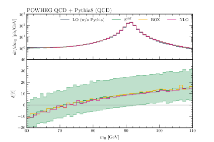
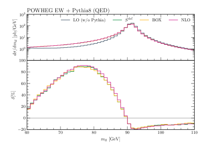
Figure 1: Invariant-mass distribution of the lepton pair. The LO result is shown along with only the QCD (left plot) and only the EW (right plot) corrections. The results of our implementation of the Powheg method without resonance improvement (labeled by $S^{\rm def}$) are compared to the Powheg-Box results (labeled by BOX) and the fixed-order NLO results. The lower plots show the relative QCD/QED corrections, where we include a scale-variation error band for the QCD correction.

For the specified setup and input parameters, we obtain $1890\pm 1$ pb for the inclusive neutral-current Drell–Yan cross section (no-cuts applied other than $m_{ll}>50~{}\text{GeV}$ at Born level) and $10941\pm 2$ pb for the inclusive charged-current Drell–Yan cross section (only a technical cut $m_{ll}>1~{}\text{GeV}$ applied as in Ref. [24]). The error of these benchmark numbers only includes the statistical error due to Monte-Carlo integration of the cross sections. The Powheg-Box results [44, 42] agree at the per mill level. All differential results discussed in the following are normalized to our total cross section results.

In Figure 1, we compare our implementation of the Powheg method for the neutral-current Drell–Yan process with the Powheg-Box implementation [42]. For the dilepton invariant-mass spectrum $m_{ll}$ without lepton–photon recombination (bare muons), we find good overall agreement with respect to QCD as well as EW corrections, where also the Pythia shower contains either only QCD or only QED radiation. We also show the fixed-order NLO QCD and EW correction to the $m_{ll}$ distribution. For all the absolute predictions shown in the following, there are QCD uncertainties due to missing higher-order corrections (typically assessed via scale variations), PDF uncertainties or non-perturbative uncertainties due to intrinsic transverse momentum of the partons within the proton, hadronization or the underlying event. In Figure 1, we show, for example, the uncertainty due to the scale variation between $\mu_{F}=\mu_{R}=2M_{\mathrm{Z}}$ and $\mu_{F}=\mu_{R}=M_{\mathrm{Z}}/2$. As can be seen, QCD uncertainties are rather flat and affect the overall normalization. In contrast, the shape of the leptonic invariant-mass or transverse mass distributions close to their peak is affected much more by EW corrections. Concerning EW corrections, QCD uncertainties for the relative corrections are negligible and not included in Figure 1. While QCD uncertainties have been extensively analyzed for a thorough understanding of the Drell–Yan process and in particular for the measurement of the W-boson mass (see for example Ref. [3, 46] and references therein), they are not relevant for the following comparison of shape differences in the distributions due to different resonance improvements and are not discussed further.

In Figure 2, we show the impact of the EW corrections on $\bar{B}$ as a function of the dilepton invariant mass $m_{ll}$. For the standard choice of the $S$ function without resonance improvement, the difference between $B$ and $\bar{B}$ has a pronounced percent-level structure around the resonance peak and is larger than 10% in the low invariant-mass tail. The results agree well with the Powheg-Box prediction. Since $\bar{B}$ depends on the choice of the $S$ functions, it has no physical meaning on the level of a fixed-order NLO calculation, where the differences in $\bar{B}$ are exactly canceled by including real radiation. However, $\bar{B}$ impacts the results within the Powheg method at the level of higher-order corrections beyond NLO which are included in the prediction. The relatively large EW corrections in $\bar{B}$ can be attributed to the resonance issue discussed in Section 2. Using $S^{\rm def}$, the wrongly assigned resonance history is responsible for moving events from the resonance peak to the tails. FSR events which are erroneously assigned as ISR events are moved below the resonance peak. ISR events which are erroneously assigned as FSR events are moved above the resonance peak. Since FSR is dominant due to the larger lepton charges, more events from the peak are moved to lower values of $m_{ll}$.

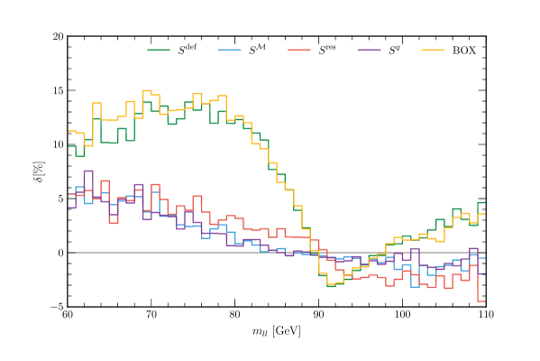
Figure 2: Relative EW corrections to $\bar{B}$ for the invariant-mass distribution of the lepton pair. Results for different choices for the underlying $S$ functions are shown, where $S^{\rm def}$, $S^{\mathcal{M}}$, $S^{\rm res}$, and $S^{q}$ are defined in Section 2. We also show the result of the Powheg-Box which agrees well with the corrections based on $S^{\rm def}$.

Indeed, defining $\bar{B}$ by distinguishing between ISR and FSR on the basis of the matrix element (labeled by $S^{\mathcal{M}}$ in Figure 2), the EW corrections in $\bar{B}$ are small and resemble the weak virtual corrections (see Figure 12 in Ref. [16]) which form a gauge-invariant subset of corrections. They grow at low dilepton invariant masses since the photon-exchange at LO starts to impact the distribution for which the $G_{\mu}$ scheme is not the optimal choice. Subtracting weak corrections, the remaining photonic corrections turn out to be at the per mill level only.

Using $S^{\rm res}$ (see Section 2) to define resonance-improved $S$ functions, the results agree with the matrix-element method at the one-percent level. Including the relevant fermion charges in the definition of $S^{q}$, the matrix-element based result $S^{\mathcal{M}}$ is reproduced within statistical fluctuations.

At the level of $\bar{B}$, NLO QCD and EW corrections are simply added in our calculation. A factorized approach, where the EW corrections are multiplicatively applied to the best QCD prediction, would lead to essentially the same result around the resonance peak, since the EW corrections are so small. The resonance-improved (physical) definition of the underlying $S$ functions seems to imply very small $\mathcal{O}(\alpha_{s}\alpha)$ corrections since already the $\mathcal{O}(\alpha)$ corrections to $\bar{B}$ are tiny around the resonance peak. The bulk of the mixed $\mathcal{O}(\alpha_{s}\alpha)$ is then contained in the interplay of photon radiation off the final-state leptons with the QCD corrections as found in Ref. [26]. Higher-order EW corrections at the level of $\bar{B}$ are certainly negligible around the Z resonance and will not exceed a few per mill even in the low invariant-mass tail (see also Ref. [16]).

Figures 3 and 4 finally quantify the impact of the choice of $S$ function on the final Powheg result including QCD and EW effects in $\bar{B}$ as well as for the generation of radiation. Pythia8 is used as a parton shower. The agreement with the Powheg-Box is at the per mill level at the resonance and differences up to 1% are observed in the tail of the distribution. As expected, the differences due to the choice of $S$ functions are reduced in the full result compared to the results for $\bar{B}$. Part of the difference is compensated by generating hardest emissions according to the Powheg method, where real photons are emitted based on the same $S$ function. However, there is a percent-level distortion of the resonance peak as shown in Figure 4, where the relative differences with respect to the default Powheg result are displayed for the different $S$ functions discussed in Section 2. Since the hardest emission generated by Powheg is mostly of QCD type, not all photonic emissions, needed to cancel the $\bar{B}$ distortion up to $\mathcal{O}(\alpha^{2})$, are generated by the Powheg method. They are added by the QED parton shower instead. The higher-order $\mathcal{O}(\alpha_{s}\alpha)$ differences observed in Figure 4 are beyond the formal accuracy of the calculation and could serve as an error estimate of the Powheg method. However, since the physical reason for the deviations can be associated to the resonance treatment, the error would be clearly overestimated if a proper resonance-improved $S$ function is used. The dominant error of the full prediction is not intrinsic to the Powheg part of the computation but depends on the accuracy of the parton-shower tool which is used. For Pythia, the difference between the matched calculation and a LO plus parton-shower calculation for the pure EW corrections only exceeds 5% of the EW corrections at invariant masses below 70 GeV. Close to the Z peak, it is approximately 1% of the LO result. Around 80 GeV, where the EW corrections are largest, it reaches 5%. Since, due to hard QCD radiation, not all first photon emissions are guaranteed to be matrix-element improved in our approach, a part of this uncertainty is also present in the full prediction. It can thus be estimated to be several per mill around the Z peak and can reach the percent level in the tails of the distribution. Our resonance improvement can be combined with a first photon-emission which always has matrix-element accuracy [46], as discussed below. In this case, the uncertainty should be further reduced to approximately 1-2% of the EW correction for a given observable.

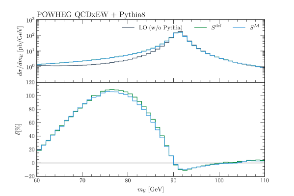
Figure 3: The invariant-mass distribution of the lepton pair is shown at LO (without parton shower) and including QCD and EW effects within the Powheg method. Pythia 8 is used as a parton shower. The lower plot shows the relative corrections with respect to the LO result. In particular, the resonance-improved result $S^{\mathcal{M}}$ is compared to the standard choice for the $S$ functions $S^{\rm def}$.

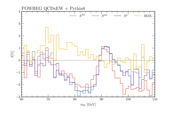
Figure 4: Same as the lower plot in Figure 3, but the relative differences are shown with respect to the result obtained with $S^{\rm def}$. We show the results for the different resonance-improved $S$ functions $S^{\rm res}$ and $S^{q}$ along with $S^{\mathcal{M}}$ and the result of the Powheg-Box.

For the charged-current Drell–Yan process, the transverse-mass distribution $m_{\rm T}$ is one of the most crucial observables for the W-boson mass measurement. In contrast to the neutral-current process, the matrix element for W-boson production cannot be separated in a gauge-invariant way into ISR and FSR parts. Also, due to the W-boson charge, there is no unambiguous definition of the fermion charges in $S^{q}$ for W-boson production. Hence, for the charged-current case, we only use $S^{\rm res}$ to improve the resonance description. In the left plot of Figure 5, for comparison, we show the transverse-mass distribution for the neutral-current process. The distribution based on $S^{\rm res}$ reproduces the best result, based on $S^{\mathcal{M}}$, within the statistical uncertainty up to $m_{\rm T}=M_{\mathrm{Z}}$. Like for the invariant-mass distribution, there is a percent-level discrepancy for $m_{\rm T}>M_{\rm Z}$. In analogy, the theoretical uncertainty due to the resonance modeling in W-boson production, which is shown in the right plot of Figure 5, can be assumed to be quite small for $m_{\rm T}<M_{\mathrm{W}}$. Above $M_{\mathrm{W}}$, the relative difference between the results using $S^{\rm def}$ and $S^{\rm res}$ is probably a good estimate for the theoretical uncertainty of the prediction according to the observations in the neutral-current case. Hence, a refined resonance improvement could further improve the prediction for the charged-current Drell–Yan process for $m_{\rm T}>M_{\mathrm{W}}$, e.g. by combining our method with the findings of  Ref. [46] as discussed below. Since there is only one radiating charged lepton in the charged-current case, the size of the resonance improvement is slightly reduced compared to the neutral-current case. At the Jacobian peak of the transverse-mass distribution, it is about 3 per mill.

This difference can be compared to the results in Figure 34 of Ref. [24], where the results of the (not resonance-improved) Powheg-Box matched to Photos [66] as a QED parton shower are compared to the results of the standard QCD only Powheg implementation with Photos. The difference is attributed to higher-order $\mathcal{O}(\alpha_{s}\alpha)$ corrections missing in the latter approach. However, the observed difference is at least partly due to the missing resonance improvement as shown in Figure 5. Hence, the true higher-order $\mathcal{O}(\alpha_{s}\alpha)$ corrections can be estimated to be much smaller.

These finding have also been addressed in Ref. [46], where a different resonance improvement has been employed which is briefly discussed in the following. If FSR is associated wrongly to ISR due to the resonance insensitive $S$ functions $S^{\rm def}$, the corresponding energy loss of the leptons is encoded already in the $\bar{B}$ function, e.g. events are moved from the Z-boson peak to lower invariant masses as shown in Figure 2. This part of the radiation is also not added as FSR in the Powheg generation of radiation, i.e. the leptons do not loose energy again due to photon emission, and NLO accuracy is reached. If, however, the first radiation is dominated by QCD emissions, the parton shower takes over and may add this FSR radiation again such that there is double counting of the energy loss of the leptons. In Ref. [46], as proposed already in Ref. [45], an extension of the Powheg method is employed which allows to generate the first emission in a resonance decay independently of the emissions in the rest of the process. Hence, the first FSR emission in Drell–Yan is always generated by Powheg and the double counting for the leptonic observables is avoided. On the other hand, the corresponding photon radiation which should be generated by Powheg ISR will still be missing since ISR is dominated by QCD radiation. However, precision measurements are based on the leptonic observables, so this drawback is phenomenologically not severe.

As an advantage, the first FSR emission is always described with Powheg precision in contrast to our approach. On the other hand, the $\bar{B}$ function reflects the physics much better if a resonance-improved $S$ functions is used such that unwanted artifacts in the higher-order corrections can be avoided from the start. In particular, our approach points towards negligible $\mathcal{O}(\alpha_{s}\alpha)$ corrections at the level of the $\bar{B}$ function. Finally, we want to stress that the two solutions to achieve resonance improvement can be easily combined to achieve all the advantages of each method and to avoid all the disadvantages of the other. In particular, the resonance-improved $S$ function discussed in detail in this work can be easily incorporated in the public Powheg version presented in Ref. [46].

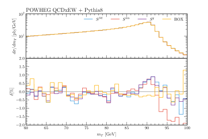
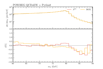
Figure 5: Transverse-mass distribution for the neutral-current (left) and charged-current (right) Drell–Yan processes. We show the differential cross section (top) and the relative corrections (bottom) with respect to the results obtained using $S^{\rm def}$ for $S^{\rm res}$, $S^{\mathcal{M}}$, $S^{q}$, and the Powheg-Box.

6 Conclusions

We have used a resonance-improved implementation of the Powheg method to investigate the NLO QCD and EW corrections to the Drell–Yan process matched to a parton shower. The importance of a proper treatment of the resonance with respect to associating the emission of photons to ISR or FSR by means of FKS $S$ functions is highlighted. Without resonance improvement, higher-order $\mathcal{O}(\alpha_{s}\alpha)$ corrections, which are beyond the formal accuracy of the Powheg method but which are artifacts of the method, enter the prediction. For the Z-boson line shape, they are at the percent level in the resonance region. For the W-boson transverse-mass distribution, they only reach several per mill. However, they are particularly important for the W-boson mass measurement at the level of a few MeV.

A proper resonance improvement of the Powheg method also leads to small NLO EW corrections in the Powheg $\bar{B}$ function. Hence, the mixed $\mathcal{O}(\alpha_{s}\alpha)$ corrections in $\bar{B}$ can also be expected to be rather small. The dominant $\mathcal{O}(\alpha_{s}\alpha)$ effects are then contained in the kinematic effects due to photon emission interleaved with QCD ISR which are particularly well described by the matrix-element improved parton shower within the Powheg method. This picture is consistent with the findings of Ref. [26], where the dominant $\mathcal{O}(\alpha_{s}\alpha)$ corrections in the pole approximation are found to arise from EW corrections in the final state combined with QCD corrections in the initial state. The resonance description can be further improved by using the resonance-improved $S$ functions within the approach discussed in Ref. [46].

On the technical side, we provide the results to use the Powheg method for calculations including massless fermions using mass regularization instead of dimensional regularization.

In the future, resonance-improved predictions for the production of weak gauge bosons at high transverse momenta recoiling against a jet are a natural next step to further improve the theoretical description of weak boson production at the LHC.

Appendix A Derivation of the soft-virtual contribution for FKS subtraction using mass regularization

In this appendix we derive the soft-virtual contribution to the cross section as given in Equation (9) in Section 3. The partonic part of the real cross section is given by

$$\hat{\sigma}_{n+1}=\int\operatorname{d}\!\Phi_{n+1}\mathcal{R}\,$$ (25)

with

$$\mathcal{R}=\frac{1}{2s}|\mathcal{M}_{n+1}|^{2}\,,$$ (26)

where $\mathcal{M}_{n+1}$ is the real-emission matrix element with massive fermions and a photon mass is introduced in potentially singular propagators. The phase space is given by

$$\operatorname{d}\!\Phi_{n+1}=\prod_{i=1}^{n}\frac{\operatorname{d}^{3}\!p_{i}}{(2\pi)^{3}2E_{i}}\frac{\operatorname{d}^{3}\!k}{(2\pi)^{3}2E}(2\pi)^{4}\delta^{(4)}\left(k_{1}+k_{2}-k-\sum_{i=1}^{n}p_{i}\right)\,,$$ (27)

where $k$ is the momentum of an emitted photon with a regulator mass $m_{\gamma}$, $E=\sqrt{m_{\gamma}^{2}+\vec{k}^{2}}$, $k_{1,2}$ are the initial state momenta, and $p_{i}$ the final-state momenta of the particles present at Born level with corresponding energies $E_{i}$.

We are concerned with the massless limit, i.e. we extract the mass singular logarithms in the real cross section and neglect the masses otherwise. Concerning soft singularities, we subtract and add the soft or eikonal approximation for the matrix element

$$|\mathcal{M}_{n+1}^{\text{(soft)}}|^{2}=-4\pi\,\alpha\,\sum_{i,j}q_{i}q_{j}\sigma_{i}\sigma_{j}\frac{k_{i}\cdot k_{j}}{(k_{i}\cdot k)(k_{j}\cdot k)}|\mathcal{M}_{n}|^{2}\,,$$ (28)

where $i,j$ runs over all external particles, $\mathcal{M}_{n}$ is the Born matrix element, and $q_{i}$, $\sigma_{i}$ are defined in Section 3. In contrast to dimensional regularization, in mass regularization also the terms with $i=j$ contribute ($k_{i}\cdot k_{i}=m_{i}^{2}$). Neglecting the soft-photon momentum in the momentum-conservation $\delta$-function, the soft approximation can be integrated analytically [51] and yields

$$\hat{\sigma}_{n+1}^{\text{(soft)}}=\frac{\alpha}{2\pi}\int\operatorname{d}\!\Phi_{n}\Bigl{(}\mathcal{B}\,\mathcal{Q}_{\text{soft}}+\sum_{\begin{subarray}{c}i,j\\ i\not=j\end{subarray}}\mathcal{B}_{ij}\mathcal{I}_{ij}\Bigr{)}$$ (29)

with the definitions given in Section 3. To obtain this result for the massless limit, the results for arbitrary masses in Ref. [51] are expanded, keeping only the mass-singular logarithms and mass-independent terms.

The real-emission contribution can now be written as

$$\hat{\sigma}_{n+1}=\hat{\sigma}_{n+1}^{\text{(soft)}}+\int\operatorname{d}\!\Phi_{n+1}\left(\frac{1}{\xi}\right)_{\!\xi_{c}}\,\,\xi\,\mathcal{R}\,,$$ (30)

where $\xi=2E/\sqrt{s}$ denotes the relative photon energy and we have defined the plus-distribution [36]

$$\int_{0}^{1}\!\operatorname{d}\!\xi\,\left(\frac{1}{\xi}\right)_{\!\xi_{c}}f(\xi)=\int_{0}^{1}\!\operatorname{d}\!\xi\,\frac{f(\xi)-f(0)\Theta(\xi_{c}-\xi)}{\xi}\,$$ (31)

for $0<\xi_{c}\leq 1$. Note, that the second term in (30) does not contain a soft singularity due to the plus-distribution such that the photon mass is no longer needed as a regulator.

Concerning the collinear singularities, according to the FKS prescription, we introduce $S$ functions to decompose the real-emission phase space

$$\int\operatorname{d}\!\Phi_{n+1}\left(\frac{1}{\xi}\right)_{\!\xi_{c}}\left(\xi\,\mathcal{R}\right)=\sum_{i=0}^{n}\,\hat{\sigma}_{i}$$ (32)

with

$$\hat{\sigma}_{i}=\int\operatorname{d}\!\Phi_{n+1}\,\,S_{i}\,\left(\frac{1}{\xi}\right)_{\!\xi_{c}}\,\,\xi\,\mathcal{R}$$ (33)

such that each $\hat{\sigma}_{i}$ contains either only the initial-state collinear singularities ($i=0$) or one final-state collinear singularity for photon emission collinear to particle $i$.

To extract the initial-state singularity, one subtracts and adds the collinear approximations for the matrix element

$$|\mathcal{M}_{n+1}^{\text{(initial,i)}}|^{2}=\frac{4\pi\,\alpha\,q_{i}^{2}}{z(k_{i}\cdot k)}\left[P_{ff}(z)-\frac{zm_{i}^{2}}{(k_{i}\cdot k)}\right]|\mathcal{M}_{n}(zk_{i})|^{2}\,,$$ (34)

where the splitting function is given by $P_{ff}(z)=\frac{1+z^{2}}{1-z}$ and $z=1-\frac{E}{E_{i}}=1-\xi$ denotes the momentum fraction of the initial-state fermion $i$ after the emission of the collinear photon. The argument of $\mathcal{M}_{n}(zk_{i})$ is given in order to state that the reduced momentum $zk_{i}$ enters the Born matrix element. The subtracted cross section is free of collinear singularities, so that the regulator masses can be taken to zero. Hence, the subtracted cross section can be expressed in terms of plus-distributions in complete analogy to dimensional regularization. In the subtraction term, the collinear limit has to be used in the momentum-conservation $\delta$-function. Hence, the angular integrals over the collinear approximation can be again analytically solved to obtain

$$\hat{\sigma}^{\text{(initial,1)}}\!=\!\frac{\alpha\,q_{1}^{2}}{2\pi}\!\!\int\prod_{i=1}^{n}\frac{\operatorname{d}^{3}\!p_{i}}{(2\pi)^{3}2E_{i}}\int_{0}^{1}\!\operatorname{d}\!z\,\!\left(\frac{1}{1-z}\right)_{\!\xi_{c}}\!(2\pi)^{4}\delta^{(4)}\left(zk_{1}+k_{2}-\sum_{i=1}^{n}p_{i}\right)\\ \times\left[-\frac{(1-z)P_{ff}(z)}{z}\log\frac{m_{1}^{2}}{2E_{1}^{2}\delta_{\text{I}}}-2\right]\frac{1}{2s}|\mathcal{M}_{n}(zk_{1})|^{2}\,,$$ (35)

where $s=(zk_{1}+k_{2})^{2}$ is the center-of-mass energy squared of the Born matrix element and the integral over the angle $\theta$ between the emitter and the photon has been restricted by $\Theta(\delta_{\text{I}}-1+\cos\theta)$ with $0<\delta_{\text{I}}\leq 2$. The choice of $\delta_{\text{I}}$ corresponds to using the plus-distribution [36]

$$\int_{-1}^{1}\!\operatorname{d}\!y\,\left(\frac{1}{1-y}\right)_{\!\delta_{\text{I}}}f(y)=\int_{-1}^{1}\!\operatorname{d}\!y\,\frac{f(y)-f(0)\Theta(\delta_{\text{I}}-1+y)}{1-y}\,$$ (36)

with $y=\cos\theta$ to define the subtracted cross section. For the corresponding hadronic cross section one finds

$$\sigma^{\text{(initial,1)}}=\int_{0}^{1}\!\operatorname{d}\!x_{1}\,\int_{0}^{1}\!\operatorname{d}\!x_{2}\,\,\mathcal{L}(x_{1},x_{2},\mu_{F})\,\hat{\sigma}^{\text{(initial,1)}}(k_{1},k_{2})\\ =\frac{\alpha\,q_{1}^{2}}{2\pi}\int_{0}^{1}\!\operatorname{d}\!\overline{x}_{1}\,\int_{0}^{1}\!\operatorname{d}\!x_{2}\,\,\!\!\int\operatorname{d}\!\Phi_{n}\int_{\overline{x}_{1}}^{1}\!\operatorname{d}\!z\,\!\left(\frac{1}{1-z}\right)_{\!\xi_{c}}\,\mathcal{L}\left(\frac{\overline{x}_{1}}{z},x_{2},\mu_{F}\right)\\ \times\left[-\frac{(1-z)P_{ff}(z)}{z}\log\frac{m_{1}^{2}}{2E_{1}^{2}\delta_{\text{I}}}-2\right]\frac{1}{2s}|\mathcal{M}_{n}(k_{1})|^{2}\,,$$ (37)

where $\overline{x}_{1}=zx_{1}$, the parton luminosity $\mathcal{L}(x_{1},x_{2},\mu_{F})=f(x_{1},\mu_{F})f(x_{2},\mu_{F})$ is given by the product of the corresponding PDFs, and $s$ is again given by the center-of-mass energy squared of the Born matrix element $\mathcal{M}_{n}$, i.e. $s=(k_{1}+k_{2})^{2}$.

The logarithm of the fermion mass is absorbed by the renormalization of the parton-distribution functions (PDFs). In mass regularization, the PDF renormalization for a quark $q$ or the corresponding anti-quark amounts to [65, 16]

$$f^{\text{ren}}(x_{1},\mu_{F})=f(x_{1},\mu_{F})-\frac{\alpha\,q_{q}^{2}}{2\pi}\int_{x_{1}}^{1}\!\operatorname{d}\!z\,\frac{1}{z}f(x_{1}/z,\mu_{F})\\ \times\left[\left(P_{ff}(z)\right)_{\!+}\log\frac{\mu^{2}_{F}}{m_{1}^{2}}-\left(P_{ff}(z)\Bigl{(}2\log(1-z)+1\Bigr{)}\right)_{\!+}+K_{ff}\right]\,,$$ (38)

where the usual plus-distribution ($\xi_{c}=1$) enters. Moreover, $\mu_{F}$ is the factorization scale and $K_{ff}=0$ in the $\overline{\text{MS}}$ scheme and $K_{ff}=K^{\text{DIS}}_{ff}$ in the DIS scheme with

$$K^{\text{DIS}}_{ff}=\left(P_{ff}(z)\left(\log\left(\frac{1-z}{z}\right)-\frac{3}{4}\right)+\frac{9+5z}{4}\right)_{\!+}\,.$$ (39)

After PDF renormalization, we find

$$\sigma^{\text{(initial,1)}}_{\text{ren}}=\frac{\alpha q_{1}^{2}}{2\pi}\int_{0}^{1}\!\operatorname{d}\!x_{1}\,\int_{0}^{1}\!\operatorname{d}\!x_{2}\,\!\int\!\operatorname{d}\!\Phi_{n}\mathcal{B}\int_{x_{1}}^{1}\!\operatorname{d}\!z\,\frac{1}{z}\mathcal{L}\left(\frac{x_{1}}{z},x_{2},\mu_{F}\right)\mathcal{G}_{1}(z)\\ +\frac{\alpha q_{1}^{2}}{2\pi}\int_{0}^{1}\!\operatorname{d}\!x_{1}\,\int_{0}^{1}\!\operatorname{d}\!x_{2}\,\!\int\!\operatorname{d}\!\Phi_{n}\,\mathcal{B}\,\mathcal{L}\left(x_{1},x_{2},\mu_{F}\right)\\ \times\left(\frac{3}{2}\log\frac{m_{1}^{2}}{\mu_{F}^{2}}-2+\left(\log\frac{m_{1}^{2}}{\mu_{F}^{2}}+1\right)\log\xi^{2}_{c}+\frac{1}{2}\log^{2}\xi^{2}_{c}\right),$$ (40)

where

$$\mathcal{G}_{1}(z)=\left[\log\frac{s\delta_{\text{I}}}{2z\mu_{F}^{2}}\left(\frac{1}{1-z}\right)_{\!\xi_{c}}+2\left(\frac{\log(1-z)}{1-z}\right)_{\!\xi_{c}}\right]\!(1-z)P_{ff}(z)\,+(1-z)-K_{ff}$$ (41)

is equivalent to the result in dimensional regularization and the second line of (40) contributes to $\mathcal{Q}_{\text{initial}}$. For the second initial-state fermion, the equivalent result is found. Concerning the electroweak corrections, the DIS scheme is usually assumed to be the best scheme choice for the current PDF sets.

Concerning the extraction of final-state collinear singularities, we follow the same strategy. In each singular region due to the emission of a photon from a final-state fermion, we subtract and add the collinear limit of the matrix element in mass regularization

$$|\mathcal{M}_{n+1}^{\text{(final,i)}}|^{2}=\frac{4\pi\alpha q_{i}^{2}}{(p_{i}\cdot k)}\left[P_{ff}(z)-\frac{m_{i}^{2}}{(p_{i}\cdot k)}\right]|\mathcal{M}_{n}(p_{i}/z)|^{2}\,,$$ (42)

where $z=\frac{E_{i}}{E_{i}+E}=\frac{\xi_{i}}{\xi_{i}+\xi}$. Again the subtracted cross section is free of singularities such that the regulator masses can be taken to zero. The subtracted cross section can be written in terms of the same plus-distributions as the result in dimensional regularization. Since the collinear limit has to be used in the momentum-conservation $\delta$-function of the subtraction term, one can analytically integrate the angular integrals to obtain

$$\hat{\sigma}^{\text{(final,i)}}\!=\!\frac{\alpha\,q_{i}^{2}}{2\pi}\!\!\int\prod_{j=1}^{n}\frac{\operatorname{d}^{3}\!p_{j}}{(2\pi)^{3}2E_{j}}\int_{0}^{1}\!\operatorname{d}\!\xi\,\left(\frac{1}{\xi}\right)_{\!\xi_{c}}(2\pi)^{4}\delta^{(4)}\Bigl{(}k_{1}+k_{2}-p_{i}/z-\sum_{\stackrel{{\scriptstyle j=1}}{{i\neq j}}}^{n}p_{j}\Bigr{)}\\ \times\left[-\frac{(1-z)P_{ff}(z)}{z}\log\frac{m_{i}^{2}}{2E_{i}^{2}\delta_{\text{O}}}-2\right]\frac{1}{2s}|\mathcal{M}_{n}(p_{i}/z)|^{2}\,,$$ (43)

where $\delta_{\text{O}}$ plays the same role as $\delta_{\text{I}}$ in restricting the range of the angular integration. After rescaling the momentum $p_{i}$ to absorb the explicit factor of $z$ in the delta-function and the matrix element, solving the $\xi$-integral yields

$$\hat{\sigma}^{\text{(final,i)}}=\frac{\alpha q_{i}^{2}}{2\pi}\int\operatorname{d}\!\Phi_{n}\,\mathcal{B}\,\left[\frac{3}{2}\log\frac{2m_{i}^{2}}{\xi_{i}^{2}s\delta_{\text{O}}}-\frac{2}{3}\pi^{2}+\frac{9}{2}+\left(\log\frac{2m_{i}^{2}}{\xi_{i}^{2}s\delta_{\text{O}}}+1\right)\log\frac{\xi^{2}_{c}}{\xi^{2}_{i}}\right]\,,$$ (44)

corresponding to $\mathcal{Q}_{\text{final}}$ defined in Section 3.

Appendix B Pythia and Powheg-Box setup

We use the default settings for Pythia 8 if not specified otherwise in the following. Concerning the matching of the Powheg results with the Pythia shower, Powheg and Pythia are both based on transverse-momentum as a shower-evolution scale. However, the precise definition of the evolution scale differs. Ignoring this difference, i.e. assuming that the Pythia and Powheg scales are the same, the simplest matching solution is to use the Powheg scale of the hardest radiation (given by SCALUP in the LHE file) as starting scale for Pythia. One can use the Pythia settings
      TimeShower:pTmaxMatch 1 SpaceShower:pTmaxMatch 1
in this case. Furthermore, one has to use
      Beams:strictLHEFscale on
to ensure that Pythia uses the starting scale provided by Powheg also when adding radiation to resonance decays. Since there is only one scale for the hardest radiation in our setup, using this flag is equivalent to implementing the Pythia function UserHooks::scaleResonance as recommended in Ref. [67].

To take the mismatch of the precise definition of the transverse-momentum based evolution scales into account, the Pythia 8 plug-in PowHegHook is provided by the Pythia authors [68]. An adapted version of this plug-in is also used in the Powheg-Box implementations Ref. [44, 42] and we follow the usage employed there. If this plug-in is used, Pythia starts its evolution at the kinematic limit and vetoes all radiation with a Powheg evolution scale above the scale of the hardest Powheg emission. This procedure is possible because the Pythia and Powheg scales are similar. A truncated shower [69] is not needed in this case according to Ref. [36, 68].

The default PowHegHook plug-in does not apply any veto in resonance decays. Therefore, one has to modify the code to enable vetoing in resonance decays. Moreover, the correct Powheg scale has to be calculated by the plug-in. In our case, the ISR scale is the transverse momentum and the FSR scale is based on the soft-collinear limit of the transverse momentum, i.e.

$$k_{T}^{2}=(p_{i}+p_{j})^{2}\frac{E_{i}}{E_{j}},$$ (45)

where the index $i$ denotes the radiated particle and $j$ denotes the emitter after radiation. The necessary changes in the code can be also found in the public implementation of the neutral-current Drell–Yan process in the Powheg-Box. Our implementation is equivalent.

The results presented in Section 5 employ the matching based on PowHegHook. The simpler matching procedure described before, shows differences at the level of 1% in the tails of the invariant-mass and transverse-mass distributions (see Figure 6). Changes in the ratios shown in Figure 4 and Figure 5 are negligible, since the parton shower matching affects the Powheg events in the same way.

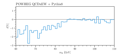
Figure 6: The plot shows the relative difference in the prediction of the invariant-mass distribution using the simple matching, where the Powheg scale is the starting scale of the shower, with respect to the vetoed shower as described in the text. Here, we have employed $S^{\mathcal{M}}$, however, the result does not depend on the $S$ functions in a significant way.

Moreover, we use the fine-structure constant in the Thomson limit:
      TimeShower:alphaEMorder 0 SpaceShower:alphaEMorder 0
Finally, we use an internal NNPDF set of Pythia:
      PDF:pSet 15
For the left panel of Figure 1, we use only the Pythia QCD shower. We switch off the QED shower by the following settings:
      SpaceShower:QEDshowerByL off SpaceShower:QEDshowerByQ off TimeShower:QEDshowerByGamma off TimeShower:QEDshowerByL off TimeShower:QEDshowerByQ off
To compare EW effect in the right panel of Figure 1, we disable the QCD shower in Pythia by the following settings:
      Checks:event off PartonLevel:Remnants off SpaceShower:QCDshower off TimeShower:QCDshower off

For performance reasons we restrict the analysis to parton level by switching off hadronization and multi-parton interactions:
      HadronLevel:all off PartonLevel:MPI off
We checked that hadronization and multi-parton interaction do not alter the results. In particular, we checked that there are no differences for the ratios of the results employing different (resonant-improved) $S$ functions.

Concerning the Powheg-Box, we use the default settings. In addition, we choose the $G_{\mu}$ scheme, $\mu_{F}=\mu_{R}=M_{\mathrm{Z}}$ and photon-induced processes are switched off:
      scheme 2 runningscale 0 photoninduced 0
Moreover, the invariant-mass cut for the neutral-current Drell–Yan process is chosen:
      mass_low 50
For the plots shown in Section 5, we use:
      olddij 1 lepaslight 1
However, the default choice for the $S$ functions or the treatment of lepton masses does not lead to noticeable differences in the differential distributions. Moreover, we choose the complex-mass scheme for the charged-current Drell–Yan process [42] by setting the corresponding flag complexmasses = .true. in init_couplings.f. If svn version r3337 or earlier is used for the neutral-current Drell–Yan process[44], one should make sure to change nubound to a value of $10^{5}$ or higher.

References

- [1] M. L. Mangano, “Production of electroweak bosons at hadron colliders: theoretical aspects,” Adv. Ser. Direct. High Energy Phys. 26 (2016) 231–253, arXiv:1512.00220 [hep-ph].
- [2] M. Baak et al., “Working Group Report: Precision Study of Electroweak Interactions,” in Proceedings, Community Summer Study 2013: Snowmass on the Mississippi (CSS2013): Minneapolis, MN, USA, July 29-August 6, 2013. 2013. arXiv:1310.6708 [hep-ph].
- [3] M. Aaboud et al. [ATLAS Collaboration], “Measurement of the -boson mass in pp collisions at TeV with the ATLAS detector,” arXiv:1701.07240 [hep-ex].
- [4] G. Altarelli, R. K. Ellis, and G. Martinelli, “Large Perturbative Corrections to the Drell-Yan Process in QCD,” Nucl.Phys. B157 (1979) 461.
- [5] R. Hamberg, W. L. van Neerven, and T. Matsuura, “A Complete calculation of the order correction to the Drell-Yan factor,” Nucl. Phys. B359 (1991) 343–405. [Erratum: Nucl. Phys.B644,403(2002)].
- [6] R. V. Harlander and W. B. Kilgore, “Next-to-next-to-leading order Higgs production at hadron colliders,” Phys. Rev. Lett. 88 (2002) 201801, arXiv:hep-ph/0201206 [hep-ph].
- [7] C. Anastasiou, L. J. Dixon, K. Melnikov, and F. Petriello, “High precision QCD at hadron colliders: Electroweak gauge boson rapidity distributions at NNLO,” Phys. Rev. D69 (2004) 094008, arXiv:hep-ph/0312266 [hep-ph].
- [8] S. Catani, L. Cieri, G. Ferrera, D. de Florian, and M. Grazzini, “Vector boson production at hadron colliders: a fully exclusive QCD calculation at NNLO,” Phys. Rev. Lett. 103 (2009) 082001, arXiv:0903.2120 [hep-ph].
- [9] K. Melnikov and F. Petriello, “Electroweak gauge boson production at hadron colliders through ,” Phys. Rev. D74 (2006) 114017, arXiv:hep-ph/0609070 [hep-ph].
- [10] R. Gavin, Y. Li, F. Petriello, and S. Quackenbush, “FEWZ 2.0: A code for hadronic Z production at next-to-next-to-leading order,” Comput. Phys. Commun. 182 (2011) 2388–2403, arXiv:1011.3540 [hep-ph].
- [11] R. Gavin, Y. Li, F. Petriello, and S. Quackenbush, “W Physics at the LHC with FEWZ 2.1,” Comput. Phys. Commun. 184 (2013) 208–214, arXiv:1201.5896 [hep-ph].
- [12] R. Boughezal, J. M. Campbell, R. K. Ellis, C. Focke, W. Giele, X. Liu, F. Petriello, and C. Williams, “Color Singlet Production at NNLO in MCFM,” arXiv:1605.08011 [hep-ph].
- [13] S. Dittmaier and M. Krämer, “Electroweak radiative corrections to W boson production at hadron colliders,” Phys. Rev. D65 (2002) 073007, arXiv:hep-ph/0109062 [hep-ph].
- [14] U. Baur, O. Brein, W. Hollik, C. Schappacher, and D. Wackeroth, “Electroweak radiative corrections to neutral current Drell-Yan processes at hadron colliders,” Phys. Rev. D65 (2002) 033007, arXiv:hep-ph/0108274 [hep-ph].
- [15] U. Baur and D. Wackeroth, “Electroweak radiative corrections to beyond the pole approximation,” Phys. Rev. D70 (2004) 073015, arXiv:hep-ph/0405191 [hep-ph].
- [16] S. Dittmaier and M. Huber, “Radiative corrections to the neutral-current Drell-Yan process in the Standard Model and its minimal supersymmetric extension,” JHEP 01 (2010) 060, arXiv:0911.2329 [hep-ph].
- [17] C. M. Carloni Calame, G. Montagna, O. Nicrosini, and A. Vicini, “Precision electroweak calculation of the charged current Drell-Yan process,” JHEP 12 (2006) 016, arXiv:hep-ph/0609170 [hep-ph].
- [18] C. M. Carloni Calame, G. Montagna, O. Nicrosini, and A. Vicini, “Precision electroweak calculation of the production of a high transverse-momentum lepton pair at hadron colliders,” JHEP 10 (2007) 109, arXiv:0710.1722 [hep-ph].
- [19] A. Arbuzov, D. Bardin, S. Bondarenko, P. Christova, L. Kalinovskaya, G. Nanava, and R. Sadykov, “One-loop corrections to the Drell-Yan process in SANC. I. The Charged current case,” Eur. Phys. J. C46 (2006) 407–412, arXiv:hep-ph/0506110 [hep-ph]. [Erratum: Eur. Phys. J.C50,505(2007)].
- [20] A. Arbuzov, D. Bardin, S. Bondarenko, P. Christova, L. Kalinovskaya, G. Nanava, and R. Sadykov, “One-loop corrections to the Drell–Yan process in SANC. (II). The Neutral current case,” Eur. Phys. J. C54 (2008) 451–460, arXiv:0711.0625 [hep-ph].
- [21] W. Placzek, S. Jadach, and M. W. Krasny, “Drell-Yan processes with WINHAC,” Acta Phys. Polon. B44 no. 11, (2013) 2171–2178, arXiv:1310.5994 [hep-ph].
- [22] Y. Li and F. Petriello, “Combining QCD and electroweak corrections to dilepton production in FEWZ,” Phys. Rev. D86 (2012) 094034, arXiv:1208.5967 [hep-ph].
- [23] G. Balossini, G. Montagna, C. M. Carloni Calame, M. Moretti, O. Nicrosini, F. Piccinini, M. Treccani, and A. Vicini, “Combination of electroweak and QCD corrections to single W production at the Fermilab Tevatron and the CERN LHC,” JHEP 01 (2010) 013, arXiv:0907.0276 [hep-ph].
- [24] S. Alioli et al., “Precision Studies of Observables in and processes at the LHC,” Eur. Phys. J. C77 no. 5, (2017) 280, arXiv:1606.02330 [hep-ph].
- [25] S. Dittmaier, A. Huss, and C. Schwinn, “Mixed QCD-electroweak corrections to Drell-Yan processes in the resonance region: pole approximation and non-factorizable corrections,” Nucl. Phys. B885 (2014) 318–372, arXiv:1403.3216 [hep-ph].
- [26] S. Dittmaier, A. Huss, and C. Schwinn, “Dominant mixed QCD-electroweak O(s) corrections to Drell-Yan processes in the resonance region,” Nucl. Phys. B904 (2016) 216–252, arXiv:1511.08016 [hep-ph].
- [27] J. H. Kühn, A. Kulesza, S. Pozzorini, and M. Schulze, “One-loop weak corrections to hadronic production of Z bosons at large transverse momenta,” Nucl. Phys. B727 (2005) 368–394, arXiv:hep-ph/0507178 [hep-ph].
- [28] J. H. Kühn, A. Kulesza, S. Pozzorini, and M. Schulze, “Electroweak corrections to hadronic production of W bosons at large transverse momenta,” Nucl. Phys. B797 (2008) 27–77, arXiv:0708.0476 [hep-ph].
- [29] A. Denner, S. Dittmaier, T. Kasprzik, and A. Mück, “Electroweak corrections to W + jet hadroproduction including leptonic W-boson decays,” JHEP 08 (2009) 075, arXiv:0906.1656 [hep-ph].
- [30] A. Denner, S. Dittmaier, T. Kasprzik, and A. Mück, “Electroweak corrections to dilepton + jet production at hadron colliders,” JHEP 06 (2011) 069, arXiv:1103.0914 [hep-ph].
- [31] A. Denner, S. Dittmaier, T. Kasprzik, and A. Mück, “Electroweak corrections to monojet production at the LHC,” Eur. Phys. J. C73 no. 2, (2013) 2297, arXiv:1211.5078 [hep-ph].
- [32] A. Gehrmann-De Ridder, T. Gehrmann, E. W. N. Glover, A. Huss, and T. A. Morgan, “Precise QCD predictions for the production of a Z boson in association with a hadronic jet,” Phys. Rev. Lett. 117 no. 2, (2016) 022001, arXiv:1507.02850 [hep-ph].
- [33] R. Boughezal, J. M. Campbell, R. K. Ellis, C. Focke, W. T. Giele, X. Liu, and F. Petriello, “Z-boson production in association with a jet at next-to-next-to-leading order in perturbative QCD,” Phys. Rev. Lett. 116 no. 15, (2016) 152001, arXiv:1512.01291 [hep-ph].
- [34] S. Catani, D. de Florian, G. Ferrera, and M. Grazzini, “Vector boson production at hadron colliders: transverse-momentum resummation and leptonic decay,” JHEP 12 (2015) 047, arXiv:1507.06937 [hep-ph].
- [35] S. Frixione and B. R. Webber, “Matching NLO QCD computations and parton shower simulations,” JHEP 06 (2002) 029, arXiv:hep-ph/0204244 [hep-ph].
- [36] S. Frixione, P. Nason, and C. Oleari, “Matching NLO QCD computations with Parton Shower simulations: the POWHEG method,” JHEP 0711 (2007) 070, arXiv:0709.2092 [hep-ph].
- [37] S. Alioli, P. Nason, C. Oleari, and E. Re, “NLO vector-boson production matched with shower in POWHEG,” JHEP 07 (2008) 060, arXiv:0805.4802 [hep-ph].
- [38] S. Alioli, P. Nason, C. Oleari, and E. Re, “A general framework for implementing NLO calculations in shower Monte Carlo programs: the POWHEG BOX,” JHEP 1006 (2010) 043, arXiv:1002.2581 [hep-ph].
- [39] S. Hoeche, Y. Li, and S. Prestel, “Drell-Yan lepton pair production at NNLO QCD with parton showers,” Phys. Rev. D91 no. 7, (2015) 074015, arXiv:1405.3607 [hep-ph].
- [40] A. Karlberg, E. Re, and G. Zanderighi, “NNLOPS accurate Drell-Yan production,” JHEP 09 (2014) 134, arXiv:1407.2940 [hep-ph].
- [41] S. Alioli, C. W. Bauer, C. Berggren, F. J. Tackmann, and J. R. Walsh, “Drell-Yan production at NNLL’+NNLO matched to parton showers,” Phys. Rev. D92 no. 9, (2015) 094020, arXiv:1508.01475 [hep-ph].
- [42] L. Barze, G. Montagna, P. Nason, O. Nicrosini, F. Piccinini, and A. Vicini, “Neutral current Drell-Yan with combined QCD and electroweak corrections in the POWHEG BOX,” Eur. Phys. J. C73 no. 6, (2013) 2474, arXiv:1302.4606 [hep-ph].
- [43] C. Bernaciak and D. Wackeroth, “Combining NLO QCD and Electroweak Radiative Corrections to W boson Production at Hadron Colliders in the POWHEG Framework,” Phys. Rev. D85 (2012) 093003, arXiv:1201.4804 [hep-ph].
- [44] L. Barze, G. Montagna, P. Nason, O. Nicrosini, and F. Piccinini, “Implementation of electroweak corrections in the POWHEG BOX: single W production,” JHEP 04 (2012) 037, arXiv:1202.0465 [hep-ph].
- [45] T. Jezo and P. Nason, “On the Treatment of Resonances in Next-to-Leading Order Calculations Matched to a Parton Shower,” JHEP 12 (2015) 065, arXiv:1509.09071 [hep-ph].
- [46] C. M. Carloni Calame, M. Chiesa, H. Martinez, G. Montagna, O. Nicrosini, F. Piccinini, and A. Vicini, “Precision Measurement of the W-Boson Mass: Theoretical Contributions and Uncertainties,” arXiv:1612.02841 [hep-ph].
- [47] S. Frixione, Z. Kunszt, and A. Signer, “Three jet cross-sections to next-to-leading order,” Nucl. Phys. B467 (1996) 399–442, arXiv:hep-ph/9512328 [hep-ph].
- [48] S. Catani and M. H. Seymour, “A General algorithm for calculating jet cross-sections in NLO QCD,” Nucl. Phys. B485 (1997) 291–419, arXiv:hep-ph/9605323 [hep-ph]. [Erratum: Nucl. Phys.B510,503(1998)].
- [49] S. Dittmaier, “A General approach to photon radiation off fermions,” Nucl.Phys. B565 (2000) 69–122, arXiv:hep-ph/9904440 [hep-ph].
- [50] S. Dittmaier, A. Kabelschacht, and T. Kasprzik, “Polarized QED splittings of massive fermions and dipole subtraction for non-collinear-safe observables,” Nucl. Phys. B800 (2008) 146–189, arXiv:0802.1405 [hep-ph].
- [51] G. ’t Hooft and M. Veltman, “Scalar One Loop Integrals,” Nucl.Phys. B153 (1979) 365–401.
- [52] L. Basso, S. Dittmaier, A. Huss, and L. Oggero, “Techniques for the treatment of IR divergences in decay processes at NLO and application to the top-quark decay,” Eur. Phys. J. C76 no. 2, (2016) 56, arXiv:1507.04676 [hep-ph].
- [53] S. Brensing, S. Dittmaier, M. Krämer, and A. Mück, “Radiative corrections to boson hadroproduction: Higher-order electroweak and supersymmetric effects,” Phys. Rev. D77 (2008) 073006, arXiv:0710.3309 [hep-ph].
- [54] J. Alwall, R. Frederix, S. Frixione, V. Hirschi, F. Maltoni, O. Mattelaer, H. S. Shao, T. Stelzer, P. Torrielli, and M. Zaro, “The automated computation of tree-level and next-to-leading order differential cross sections, and their matching to parton shower simulations,” JHEP 07 (2014) 079, arXiv:1405.0301 [hep-ph].
- [55] J. Alwall et al., “A Standard format for Les Houches event files,” Comput. Phys. Commun. 176 (2007) 300–304, arXiv:hep-ph/0609017 [hep-ph].
- [56] T. Sjostrand, S. Mrenna, and P. Z. Skands, “A Brief Introduction to PYTHIA 8.1,” Comput. Phys. Commun. 178 (2008) 852–867, arXiv:0710.3820 [hep-ph].
- [57] T. Sjostrand, S. Mrenna, and P. Z. Skands, “PYTHIA 6.4 Physics and Manual,” JHEP 0605 (2006) 026, arXiv:hep-ph/0603175 [hep-ph].
- [58] A. Buckley, J. Butterworth, L. Lonnblad, D. Grellscheid, H. Hoeth, J. Monk, H. Schulz, and F. Siegert, “Rivet user manual,” Comput. Phys. Commun. 184 (2013) 2803–2819, arXiv:1003.0694 [hep-ph].
- [59] A. Denner, S. Dittmaier, M. Roth, and D. Wackeroth, “Predictions for all processes fermions + gamma,” Nucl. Phys. B560 (1999) 33–65, arXiv:hep-ph/9904472 [hep-ph].
- [60] A. Denner, S. Dittmaier, M. Roth, and L. H. Wieders, “Electroweak corrections to charged-current fermion processes: Technical details and further results,” Nucl. Phys. B724 (2005) 247–294, arXiv:hep-ph/0505042 [hep-ph]. [Erratum: Nucl. Phys.B854,504(2012)].
- [61] NNPDF Collaboration, R. D. Ball, V. Bertone, S. Carrazza, L. Del Debbio, S. Forte, A. Guffanti, N. P. Hartland, and J. Rojo, “Parton distributions with QED corrections,” Nucl. Phys. B877 (2013) 290–320, arXiv:1308.0598 [hep-ph].
- [62] NNPDF Collaboration, S. Carrazza, “Towards the determination of the photon parton distribution function constrained by LHC data,” PoS DIS2013 (2013) 279, arXiv:1307.1131 [hep-ph].
- [63] NNPDF Collaboration, S. Carrazza, “Towards an unbiased determination of parton distributions with QED corrections,” in Proceedings, 48th Rencontres de Moriond on QCD and High Energy Interactions, pp. 357–360. 2013. arXiv:1305.4179 [hep-ph].
- [64] A. Buckley, J. Ferrando, S. Lloyd, K. Nordström, B. Page, M. Rüfenacht, M. Schönherr, and G. Watt, “LHAPDF6: parton density access in the LHC precision era,” Eur. Phys. J. C75 (2015) 132, arXiv:1412.7420 [hep-ph].
- [65] K. P. O. Diener, S. Dittmaier, and W. Hollik, “Electroweak higher-order effects and theoretical uncertainties in deep-inelastic neutrino scattering,” Phys. Rev. D72 (2005) 093002, arXiv:hep-ph/0509084 [hep-ph].
- [66] N. Davidson, T. Przedzinski, and Z. Was, “PHOTOS Interface in C++: Technical and Physics Documentation,” Comput. Phys. Commun. 199 (2016) 86–101, arXiv:1011.0937 [hep-ph].
- [67] T. Jezo, J. M. Lindert, P. Nason, C. Oleari, and S. Pozzorini, “An NLO+PS generator for and production and decay including non-resonant and interference effects,” Eur. Phys. J. C76 no. 12, (2016) 691, arXiv:1607.04538 [hep-ph].
- [68] “Powheg merging.” https://web.archive.org/web/20170120102438/http://home.thep.lu.se/~torbjorn/pythia82html/POWHEGMerging.html. Accessed: 2017-01-20.
- [69] P. Nason, “A New method for combining NLO QCD with shower Monte Carlo algorithms,” JHEP 11 (2004) 040, arXiv:hep-ph/0409146 [hep-ph].