Constraining Superfluidity in Dense Matter from the Cooling of
Isolated Neutron Stars

Abstract

We present a quantitative analysis of superfluidity and superconductivity in dense matter from observations of isolated neutron stars in the context of the minimal cooling model. Our new approach produces the best fit neutron triplet superfluid critical temperature, the best fit proton singlet superconducting critical temperature, and their associated statistical uncertainties. We find that the neutron triplet critical temperature is likely $2.09^{+4.37}_{-1.41}\times 10^{8}$ K and that the proton singlet critical temperature is $7.59^{+2.48}_{-5.81}\times 10^{9}$ K. However, we also show that this result only holds if the Vela neutron star is not included in the data set. If Vela is included, the gaps increase significantly to attempt to reproduce Vela’s lower temperature given its young age. Further including neutron stars believed to have carbon atmospheres increases the neutron critical temperature and decreases the proton critical temperature. Our method demonstrates that continued observations of isolated neutron stars can quantitatively constrain the nature of superfluidity in dense matter.

I Introduction

Neutron stars, the remnants of the gravitational collapse of $\sim{8}$ to $20~{}\mathrm{M}_{\odot}$ main-sequence stars, contain matter with densities at least several times larger than the densities at the center of atomic nuclei Lattimer and Prakash (2001). Matter at these densities is difficult to probe in the laboratory, except at high temperatures, which confounds the extraction of dense matter properties from experiment. Thus, neutron stars are a unique laboratory for the study of dense and strongly-interacting matter.

Current constraints from neutron star mass and radius observations determine the equations of state of dense matter (EOS) above the nuclear saturation densities to within about a factor of two (see recent constraints in Refs. Steiner et al. (2015); Nättilä et al. (2016) or an alternate perspective in Ref. Ozel and Freire (2016)). Recent progress in nuclear theory constrains the energy per baryon of neutron matter at the saturation density to within a few MeV Gandolfi et al. (2015). However, the EOS alone is not enough to fully describe dense matter. Almost all neutron star observables also require some knowledge of how energy and momentum are transported in dense matter. Transport properties, in turn, are strongly affected by the presence of superconductivity and superfluidity Page et al. (2014).

At the end of a supernova, the neutron star is born with a core temperature $\sim$ $10^{11}$ K, and, in some cases, a measurable velocity with respect to the remnant. Except for a thin shell at the surface, the neutron star becomes isothermal after a few hundred years. In isolated neutron stars without a companion, the temperature decreases (unless heated by magnetic field dissipation or some dark matter-related process) at a rate determined by the nature of dense matter Page et al. (2004); Yakovlev and Pethick (2004); Page and Reddy (2006). In the first $10^{5}$ years, cooling is dominated by the emission of neutrinos from the core, after which photon emission from the surface takes over. The neutrino rates strongly depend on the nature of neutron superfluidity and proton superconductivity. Thus, if one obtains temperature and age estimates from a number of cooling neutron stars, the comparison of theoretical models to data results in a constraint on the nature of superfluidity in dense matter.

II Method

There are several isolated neutron stars where age estimates are available and where x-ray data provides an estimate of the surface temperature. The extraction of the surface temperature, however, depends on the composition of the atmosphere. Older neutron stars are expected to have atmospheres made of iron-peak elements and these atmospheres are well fit by black body models giving black body radii in the range of 10$-$13 km expected from theoretical models Steiner et al. (2016). The inferred radii from black body fits to younger stars are often much smaller than expected, leading to the idea that younger isolated neutron stars may have light-element atmospheres, and hydrogen (H) atmosphere fits to the data often result in neutron star radii closer to what is expected. For most objects, only black body and H atmosphere fits to the x-ray data are available.

The temperature profile of the star depends on the composition of the envelope, which is the region between the photosphere and a boundary density near $\rho_{b}=10^{10}~{}\mathrm{g}/\mathrm{cm}^{3}$. This boundary density is defined so that the luminosity at this boundary is equal to the total luminosity of the star. In the case of a light-element atmosphere, the presence of light elements in the envelope can modify the inferred surface temperature. Light-element envelopes are not expected with iron-peak atmospheres described by black body models, as light elements in the envelope will inevitably make their way to the surface.

Similar to the procedure used in Ref. Page et al. (2004), we use the temperatures and luminosities implied by H atmosphere fits to the x-ray spectra for younger stars (less than about $10^{5}$ years) in which black body radii are too small to be realistic. In older stars, we use temperatures and luminosities obtained by blackbody fits to the x-ray spectra. The observational data set is summarized in Table 1. In the case of PSR J2043, we use the results from an H atmosphere fit because no blackbody fit was available.

The true x-ray spectrum of an isolated neutron star is not that of a black body. Modeling heat transport in hydrostatic equilibrium, Ref. Gudmundsson et al. (1983) found one can obtain a simple relationship between the effective surface temperature which depends on the amount of light elements in the envelope and the temperature at the base of the envelope, $T_{b}=T(\rho_{b})$. This relationship simplifies the calculation considerably, allowing one to connect envelope models on top of a neutron star interior Page et al. (2004). Younger stars may have light elements which affects the surface temperature, but older stars which have heavy element photospheres are not expected to have light element envelopes (as otherwise the light elements in the envelope would move towards the surface). The work in Ref. Gudmundsson et al. (1983) was updated in Ref. Potekhin et al. (1997) and our neutron star cooling model uses this work to determine the effective surface temperature and luminosity as a function of the temperature at the base of the envelope. We vary the amount of light elements in the envelope in all neutron stars less than $10^{5}$ years old, which is consistent with the notion that neutron star atmospheres evolve from light elements to iron-peak elements over time through nuclear fusion.

We also do not include any stars with magnetic fields larger than $10^{14}$ G in our data set, as the magnetic field has a strong impact on the atmosphere and may cause strong variations of the temperature on the surface which our model cannot accurately describe Potekhin (2014). In some cases, H atmosphere fits to x-ray spectra imply magnetic fields on the order of $10^{12}$ G, but we assume that there is no modification to the surface temperature or luminosity from these fields. In particular, we assume the temperature distribution is uniform across the neutron star surface.

There are a few objects for which neither H nor black body atmospheres imply a realistic neutron star radius, but where carbon atmospheres fit well. This is the case for the neutron star located in Cassiopeia A and XMMU J1732 located in HESS J1731$-$347, which we include in our analysis along with the possibility that they also may contain light elements in their envelopes.

If a neutron star can be associated with a nearby supernova remnant and its proper motion can be measured, one can determine the kinetic age, $t_{\mathrm{kin}}$. Alternatively, pulsar ages can be estimated from the spin-down timescale, $t_{\mathrm{sd}}=P/(2\dot{P})$, an age estimate assuming an evolution with a dipolar magnetic field. Spin-down ages can be measured precisely, but they disagree with kinetic ages by a factor of 3 or more Page et al. (2009), thus we assume a factor of 3 uncertainty in $t_{\mathrm{sd}}$. We presume kinetic ages are more accurate than spin-down ages, but this is not certain.

Star	$\log_{10}(t_{\rm{sd}}/\mathrm{yr})$	$B$ (G)	$\log_{10}(T^{\infty}/\mathrm{K})$	atmos.	$\log_{10}(L^{\infty})$	mass	radius	Ref.
	or $\log_{10}(t_{\rm{kin}}/\mathrm{yr})$			model	$\mathrm{erg}/\mathrm{s}$	($M_{\odot}$)	(km)
Cas A NS	2.52 (observed) Fesen et al. (2006)	$8\times 10^{10}$	$6.26^{+0.02}_{-0.02}$	C	$33.63^{+0.08}_{-0.08}$	$1.4^{*}$	12-15	Ho and Heinke (2009)
			$6.447^{+0.012}_{-0.012}$	H		$1.4^{*}$	4	Ho and Heinke (2009)
			$6.653^{+0.007}_{-0.007}$	BB		$1.4^{*}$	$<$ 1	Ho and Heinke (2009)
PSR J1119$-$6127	3.20 (s) Kumar et al. (2012)	$4.1\times 10^{13}$	$6.09^{+0.08}_{-0.08}$	HA	$33.32^{+0.14}_{-0.14}$	$1.4^{*}$	10∗	Safi-Harb and Kumar (2008)
			$6.39^{+0.02}_{-0.02}$	BB	$33.39^{+0.11}_{-0.11}$	$1.4^{*}$	$2.7{\pm}0.7$	Safi-Harb and Kumar (2008)
RX J0822$-$4247	$3.57^{+0.04}_{-0.04}$ (k)	$\sim 10^{12}$	$6.24^{+0.04}_{-0.04}$	HA	$33.93^{+0.08}_{-0.08}$	$1.4^{*}$	10∗	Zavlin et al. (1999)
			$6.65^{+0.04}_{-0.04}$	BB	$33.75^{+0.15}_{-0.15}$	$1.4^{*}$	$\approx$2	Zavlin et al. (1999)
1E 1207.4$-$5209++	$3.85^{+0.48}_{-0.48}$ (k) Zavlin et al. (2000); Roger et al. (1988)	$3\times 10^{12}$	$6.21^{+0.07}_{-0.07}$	HA	$33.50^{+0.24}_{-0.24}$	$1.4^{*}$	10∗	Pavlov et al. (2002)
			$6.48^{+0.01}_{-0.01}$	BB	$33.29^{+0.59}_{-0.59}$	$1.4^{*}$	$<$ 1.5	Mereghetti et al. (1996); Zavlin et al. (1998)
PSR J1357$-$6429	3.86 (s)	$8{\times}10^{12}$	$5.88^{+0.04}_{-0.04}$	HA	$32.63^{+0.17}_{-0.17}$	$1.5-1.6$	10∗	Zavlin (2007a)
			$6.23^{+0.05}_{-0.05}$	BB	$33.56^{+0.20}_{-0.20}$	$1.5-1.6$	$2.5{\pm}0.5$	Zavlin (2007a)
RX J0002+6246†	$3.96^{+0.08}_{-0.08}$ (k)		$6.03^{+0.03}_{-0.03}$	HA	$33.21^{+0.13}_{-0.13}$			Page et al. (2004); Pavlov et al. (2004)
			$6.15^{+0.11}_{-0.11}$	BB	$32.5^{+0.32}_{-0.32}$			Page et al. (2004); Pavlov et al. (2004)
PSR B0833$-$45	$3.97^{+0.23}_{-0.23}$ (k) Tsuruta et al. (2009)	$3{\times}10^{12}$	$5.83^{+0.02}_{-0.02}$	HA	$32.58^{+0.04}_{-0.04}$	$1.4^{*}$	13	Pavlov et al. (2001)
			$6.18^{+0.02}_{-0.02}$	BB	$32.16^{+0.12}_{-0.12}$	$1.4^{*}$	$2.1{\pm}0.2$	Pavlov et al. (2001)
PSR B1706$-$44	4.24 (s) Gotthelf et al. (2002)	$3{\times}10^{12}$	$5.80^{+0.13}_{-0.13}$	HA	$32.37^{+0.56}_{-0.56}$	$1.45-1.59$	13	McGowan et al. (2004)
			$6.22^{+0.04}_{-0.04}$	BB	$32.78^{+0.30}_{-0.30}$	$1.4^{*}$	$<6$	Gotthelf et al. (2002)
XMMU J1732$-$344	$4.43^{+0.17}_{-0.43}$ (k) Tian et al. (2008)	$\sim 10^{10-11}$	$6.25^{+0.01}_{-0.0045}$	C	$33.99^{+0.04}_{-0.02}$			Klochkov et al. (2015)
PSR J0538+2817∥	$4.47^{+0.05}_{-0.06}$ (s) Kramer et al. (2003)	$\sim 10^{12}$	$6.05^{+0.10}_{-0.10}$	HA	$33.10^{+0.50}_{-0.50}$	$1.4^{*}$	10.5	Zavlin and Pavlov (2004)
			$6.327^{+0.007}_{-0.007}$	BB		$1.4^{*}$	$<$ 2	McGowan et al. (2003)
PSR B2334+61	4.61 (s)	$\sim 10^{10-12}$	$5.68^{+0.17}_{-0.17}$	HA	$32.70^{+0.68}_{-0.68}$	$1.4^{*}$	10-13	McGowan et al. (2006)
			$6.02^{+0.19}_{-0.19}$	BB		$1.4^{*}$	$<$ 2	McGowan et al. (2006)
PSR B0656+14	5.04 (s) Zavlin (2007b)	$5{\times}10^{12}$ Mignani et al. (2015)	$5.71^{+0.03}_{-0.04}$	BB	$32.58^{+0.40}_{-0.40}$	$1.4^{*}$	12-17	Possenti et al. (1996)
PSR J1740+1000	5.06 (s) McLaughlin et al. (2002)	$1.8{\times}10^{12}$	$6.04^{+0.01}_{-0.01}$	BB	$32.15^{+0.05}_{-0.05}$			Kargaltsev et al. (2012) Viganò et al. (2013)
PSR B0633+1748	5.53 (s)		$5.75^{+0.04}_{-0.05}$	BB	$31.18^{+0.33}_{-0.33}$	$1.4^{*}$	10∗	Halpern and Wang (1997)
RX J1856.4$-$3754‡	$5.70^{+0.05}_{-0.25}$ (k) Ho (2007)	$4{\times}10^{12}$	$5.75^{+0.15}_{-0.15}$	BB	$31.56^{+0.12}_{-0.12}$		14	Pons et al. (2002); Burwitz et al. (2003)
PSR B1055$-$52§	5.73 (s)	4${\times}10^{12}$	$5.88^{+0.08}_{-0.08}$	BB	$32.57^{+0.52}_{-0.52}$	$1.4^{*}$	13	Pavlov and Zavlin (2003)
PSR J2043+2740¶	6.08 (s)	$4\times 10^{11}$	$5.64^{+0.08}_{-0.08}$	HA	$29.62^{+0.52}_{-0.52}$		10∗	Zavlin (2007b)
PSR J0720.4-3125	$6.11$ (s) de Vries et al. (2004)	$~{}10^{13}$ Kaplan et al. (2002)	$5.75^{+0.20}_{-0.20}$	BB	$31.89^{+0.52}_{-0.52}$	$1.4^{*}$	11-13	Kaplan et al. (2003)

Table 1: The data set used in the current work is adapted from the earlier work in Refs. Page et al. (2004); Viganò et al. (2013) and Lim et al. (2017). As in Ref. Page et al. (2004) we favor kinetic ages over spin-down ages where possible. The letters ‘s’ and ‘k’ in column 2 denote characteristic spin down age and kinetic age, respectively. References are given in column 2 only where our ages differ from the values used in Ref. Page et al. (2004). We use  H atmosphere (HA) fits to stars less than $10^{5}$ years and blackbody (BB) fits for older stars. In some of the H atmosphere fits, a magnetic field was used (either as a fixed value or as a fit parameter), and this is indicated in the fourth column (mHA). Notes: $(*)$ This value was assumed not derived. $(\|)$ For the H atmosphere fit, we use the redshifted temperature from Ref. Zavlin and Pavlov (2004), $10^{6.04}$, instead of the value reported as $10^{5.94}$ in Ref. Lim et al. (2017). $(\ddagger)$ As in Ref. Page et al. (2004), we use a range determined by the colder blackbody component from Ref. Pons et al. (2002) and the warmer blackbody component in Ref. Burwitz et al. (2003). $(\mathsection)$ We have used the updated information from Ref. Pavlov and Zavlin (2003) as in Ref. Lim et al. (2017) over the values in Ref. Page et al. (2004). $(\mathparagraph)$ We use a H atmosphere fit for this source since a blackbody fit is not available. $(5)$ As in Ref. Page et al. (2004) we use a range determined by the cold and warm components from the blackbody model in Ref. Kaplan et al. (2003). $(\dagger)$ Ref. Esposito et al. (2008) claims this is not a neutron star. $(++)$ As discussed in Ref. Page et al. (2004), Ref. Zavlin et al. (2004) suggests that this star may be accreting due to its spin-down behavior.

We employ the minimal cooling model from Ref. Page et al. (2004), assuming that the neutron star is made entirely of neutrons, protons, and leptons, and that the direct Urca process does not occur. When the direct Urca process does not operate, the neutron star cooling depends only weakly on the neutron star mass and the bulk thermodynamics of matter which is determined by the equation of state. If the direct Urca process does occur, then the cooling curves would depend strongly on the equation of state and individual neutron star masses. In this work, we assume the Akmal-Pandharipande-Ravenhall (APR) Akmal et al. (1998) equations of state and we also set the mass of all isolated neutron stars to 1.4 $\mathrm{M}_{\odot}$ (we will find below that the data does not require the direct Urca process, except possibly in the case of the Vela pulsar). We assume no additional cooling occurs due from presence of deconfined quarks, Bose condensates, or exotic (i.e., heavy) hadrons. The simplification provided by the minimal cooling model is important because it allows us to decrease our parameter space which is already relatively large (as described below). We also ignore any possible effects on the cooling from rotation.

In the minimal model, the principal unknown quantities in dense matter which impact neutron star cooling are the neutron superfluid and proton superconducting gaps. Superfluidity and superconductivity exponentially suppress the specific heat and modify the neutrino emissivities in dense matter (for a review see Ref. Page et al. (2014)). These effects begin when the temperature of the neutron star cools below the critical temperature. In the original BCS theory of superconductivity, the critical temperature and the value of the gap at zero temperature are related by $\Delta$$(\text{T}=0)$$\simeq 1.8\,k_{B}T_{c}$. The BCS approximation to superconductivity does not necessarily apply in the strongly-interacting nucleonic fluid, but we retain the standard practice of assuming that the BCS relation is approximately correct.

Neutron superfluidity in the singlet (${}^{1}\mathrm{S}_{0}$) channel is present in the neutron star crust, but the critical temperatures are too large to be constrained by the data of neutron stars older than a few hundred years. Proton singlet superconductivity in the outer core and neutron triplet ³P₂ superfluidity in the inner core, on the other hand, are the most important parameters in the minimal cooling model and can be constrained by neutron stars with the ages found in our data set. Superfluid gaps suppress heat capacity for temperatures well below $T_{c}$ (but increase heat capacity at temperature just below $T_{c}$). Superfluidity and superconductivity also allow a new neutrino emission process induced by the formation of Cooper pairs. This cooling process is included, along with the correction from suppression in the vector channel Flowers et al. (1976); Leinson and Perez (2006); Leinson and Pérez (2006); Steiner and Reddy (2009). We also include the axial anomalous contribution to the pair-breaking emissivity from Ref. Leinson (2010).

Theoretical calculations of the neutron and proton critical temperatures in the neutron star core appear approximately as Gaussian functions of the Fermi momentum Page et al. (2014). Pairing is suppressed at low densities as the interparticle spacing is increased, and also suppressed at high densities as the repulsion between nucleons quenches the attractive interaction. In this work, we assume that both the proton singlet and neutron triplet critical temperatures can be described by the Gaussian form

$$T_{c}(k_{F})=T_{c,\mathrm{peak}}\exp\left[\frac{\left(k_{F}-k_{F,\mathrm{peak}}\right)^{2}}{2\Delta k_{F}^{2}}\right]$$ (1)

with parameters $T_{c,\mathrm{peak}}$, $k_{F,\mathrm{peak}}$ and $\Delta k_{F}$.

To avoid overcounting models where the gaps vanish, we constrain $k_{F,p,\mathrm{peak}}$ and $k_{F,n,\mathrm{peak}}$ to lie between the crust-core transition (taken to be at $n_{B}=0.09~{}\mathrm{fm}^{-3}$) and the central density of a $1.4~{}\mathrm{M}_{\odot}$ neutron star (at $n_{B}=0.545~{}\mathrm{fm}^{-3}$). This implies $0.481~{}\mathrm{fm}^{-3}<k_{F,p,\mathrm{peak}}<1.304~{}\mathrm{fm}^{-3}$ and $1.418~{}\mathrm{fm}^{-3}<k_{F,n,\mathrm{peak}}<2.300~{}\mathrm{fm}^{-3}$. To avoid overcounting models where the gap is nearly independent of density, we also enforce $\Delta k_{F,p}<1.304~{}\mathrm{fm}^{-3}$ and $\Delta k_{F,n}<2.300~{}\mathrm{fm}^{-3}$. Finally, we constrain our critical temperatures to be smaller than $10^{10}$ K because the fit is insensitive to larger values.

In the case where one is fitting a model to data with small uncertainties in the independent variable, the $\chi^{2}$ procedure gives an unambiguous procedure to determine the best fit assuming that the data points are statistically independent and have a normally distributed uncertainty in the dependent variable. When the data points are presented in a two-dimensional plane with comparable uncertainties in both axes, there is no unique “correct” fitting procedure (this conclusion holds in both the frequentist and Bayesian paradigms). In the frequentist picture, the lack of a unique fitting procedure has led to the use of several methods including orthogonal least squares, orthogonal regression, and reduced major axis regression Isobe et al. (1990). Several of these procedures are often referred to by different names. Reduced major axis regression is also referred to as geometric mean regression in Ref. Draper and Yang (1997) and a linear version obtaining the so-called “impartial line” was first used in Ref. Strömberg (1990). This ambiguity is part of the reason why more quantitative fits to neutron star cooling data have not yet been performed before this work.

We choose to proceed using Bayesian inference, with

$$P(M|D)\propto P(D|M)P(M)$$ (2)

where $P(M)$ is the prior distribution for the model $M$ (which in our case has six parameters for superfluidity or superconductivity and one parameter for the envelope composition of each star) and $P(D|M)$ is the likelihood function obtained from the neutron star cooling data. The quantity $P(M|D)$ is the probability distribution that we want to obtain, the probability of the theoretical model given the data. In the Bayesian picture, the non-uniqueness in the fitting procedure described above is manifest in the undetermined prior distribution which one must choose to proceed.

Because the uncertainties in the neutron star cooling data are often presented in terms of the logarithms of temperature and time, we choose to write the likelihood in terms of new variables $\hat{t}$ and $\hat{T}$,

$$\widehat{t} \equiv \frac{1}{5}\log_{10}\left(\frac{t}{10^{2}~{}\mathrm{yr}}\right)\quad\mathrm{and}$$

$$\widehat{T} \equiv \frac{1}{2}\log_{10}\left(\frac{T}{10^{5}~{}\mathrm{K}}\right)$$ (3)

which are defined so that typical values are between 0 and 1.

We assume that our data set is Gaussian in both variables $\widehat{t}$ and $\widehat{T}$, and can thus be specified as $\widehat{t}_{j}$, $\widehat{T}_{j}$, $\delta\widehat{t}_{j}$, and $\delta\widehat{T}_{j}$. (Our uncertainties are sufficiently small that the distinction between normal and log-normal distributions will not strongly impact our qualitative results.) The composition of the envelope is parameterized by a quantity $\eta$ which takes values from 0 to $10^{-7}$, larger values representing a larger contribution from light elements Potekhin et al. (1997). The cooling code computes three different cooling curves, for $\eta=0$, $\eta=10^{-12}$, and $\eta=10^{-7}$ and results for other values of $\eta$ are obtained through linear interpolation. The likelihood function is

$$\cal{L}_{\mathrm{H}} \propto \prod_{j}{\int d\widehat{t}{\sqrt{\left\{\left[\frac{d\widehat{T}(\eta_{j},\widehat{t})}{d\widehat{t}}\right]^{2}+1\right\}}}}\exp\left\{\frac{-\left[\widehat{t}-\widehat{t}_{j}\right]^{2}}{2\left(\delta\widehat{t}_{j}\right)^{2}}\right\}$$ (4)

$$\times\exp\left\{\frac{-\left[\widehat{T}\left(\eta_{j},\widehat{t}\right)-\widehat{T}_{j}\right]^{2}}{2\left(\delta\widehat{T}_{j}\right)^{2}}\right\}\,.$$

where the product runs over all of the neutron stars in the data set. The overall normalization is unspecified and is not necessary for our results. For older neutron stars with spectra well fit by a blackbody spectrum, $\eta=0$, corresponding to the assumption that a heavy-element atmosphere implies no light elements in the envelope. Note that this likelihood function reduces exactly to the likelihood function for the traditional $\chi^{2}$ procedure in the limiting cases that one of the two variables has a small uncertainty. The square root operates as a line element, specifying how one defines a distance when integrating the cooling curve along the data. The ambiguity in defining this distance is the exact same as the choice in using different frequentist regression techniques. Our approach makes this ambiguity explicit.

This technique is very similar to the recent determination of the mass-radius curve given neutron star mass and radius observations (the formalism was first developed in Ref. Steiner et al. (2010) and most recently updated in Ref. Steiner et al. (2016)). There are two significant differences. First, the term under the square root was ignored, appropriate because the radius depends only very weakly on the neutron star mass. Second, the data in that case is not Gaussian in either mass or radius so a more complicated probability distribution was used rather than the product of two Gaussians employed in this work.

In practice, the cooling curves are specified as arrays, $\widehat{T}(\eta,\widehat{t})\rightarrow[\widehat{T}_{k}(\eta),\widehat{t}_{k}]$ and finite differencing gives the derivative $[d\widehat{T}(\eta)/d\widehat{t}]_{k}$. To a good approximation we can replace the integral by a sum

$$\cal{L} \propto \prod_{j}{\sum_{k}{\sqrt{\left\{\left[\frac{d\widehat{T}(\eta_{j})}{d\widehat{t}}\right]_{k}^{2}+1\right\}}}}\exp\left\{\frac{-\left[\widehat{t}_{k}-\widehat{t}_{j}\right]^{2}}{2(\delta\widehat{t}_{j})^{2}}\right\}$$ (5)

$$\times\exp\left\{\frac{-\left[\widehat{T}_{k}(\eta_{j})-\widehat{T}_{j}\right]^{2}}{2(\delta\widehat{T}_{j})^{2}}\right\}\,.$$

over a uniform grid in $\hat{t}\in[0,1]$. In this context, one can see the purpose for the term under the square root sign: in regions where the cooling curve is nearly vertical, the data covers fewer grid points than in regions where the curve is nearly horizontal. The term under the square root compensates for this, ensuring portions of the cooling curve which are nearly vertical get extra weight. This reweighting is relatively weak in comparison to the data, which exponentially affects the likelihood. We choose a grid of size 100 but increasing the number of grid points will not affect our basic conclusions. When we fit luminosities rather than temperatures, we can just replace $\widehat{T}$ with $\widehat{L}\equiv(1/4)\mathrm{log}_{10}[L/(10^{30}~{}\mathrm{erg}/\mathrm{s})]$.

The Markov chain Monte Carlo begins with an initial guess for the six superfluid parameters ($T_{c,\mathrm{peak},n}$, $k_{F,\mathrm{peak},n}$, $\Delta k_{F,n}$, $T_{c,\mathrm{peak},p}$, $k_{F,\mathrm{peak},p}$, $\Delta k_{F,p}$) and the envelope composition parameters. A new set of gaps and envelope compositions is randomly selected and the new likelihood is computed. The step is rejected or accepted according to the Metropolis algorithm. The autocorrelation length of all of the parameters is computed and the data is block averaged to ensure the uncertainties in the parameters are properly estimated.

Quantity	Value and 1$-\sigma$ uncertainty
	w/o Vela or carbon	w/o carbon	All
$\log_{10}T_{c,\mathrm{peak},n}$	$8.48\pm 0.57$	$9.11\pm 0.19$	$9.61\pm 0.22$
$k_{F,\mathrm{peak},n}~{}(\mathrm{fm}^{-1})$	$1.70\pm 0.12$	$1.924\pm 0.089$	$1.750\pm 0.082$
$\Delta k_{F,n}~{}(\mathrm{fm}^{-1})$	$0.21\pm 0.09$	$1.980\pm 0.076$	$1.80\pm 0.10$
$\log_{10}T_{c,\mathrm{peak},p}$	$8.57\pm 0.60$	$8.81\pm 0.81$	$8.72\pm 0.45$
$k_{F,\mathrm{peak},p}~{}(\mathrm{fm}^{-1})$	$0.67\pm 0.10$	$0.937\pm 0.086$	$1.02\pm 0.10$
$\Delta k_{F,p}~{}(\mathrm{fm}^{-1})$	$0.33\pm 0.12$	$0.145\pm 0.061$	$0.219\pm 0.067$
$\log_{10}\eta_{\mathrm{Cas\>A}}$			$-9.52\pm 0.87$
$\log_{10}\eta_{\mathrm{XMMU\>J1732}}$			$-9.14\pm 0.70$
$\log_{10}\eta_{\mathrm{PSR\>J1119}}$	$-14.3\pm 1.4$	$-16.00\pm 0.77$	$16.56\pm 0.63$
$\log_{10}\eta_{\mathrm{RXJ\>0822}}$	$-8.80\pm 0.68$	$-9.80\pm 0.64$	$-9.97\pm 0.84$
$\log_{10}\eta_{\mathrm{1E\>1207}}$	$-9.57\pm 0.87$	$-10.8\pm 1.0$	$-10.22\pm 0.71\$
$\log_{10}\eta_{\mathrm{PSR\>J1357}}$	$-9.30\pm 0.81$	$-9.18\pm 0.50$	$-9.58\pm 0.88$
$\log_{10}\eta_{\mathrm{RX\>J0002}}$	$-16.36\pm 0.68$	$-16.90\pm 0.39$	$-16.40\pm 0.61$
$\log_{10}\eta_{\mathrm{PSR\>B0833}}$		$-8.29\pm 0.49$	$-8.65\pm 0.67$
$\log_{10}\eta_{\mathrm{PSR\>B1706}}$	$-9.35\pm 0.79$	$-8.9\pm 1.1$	$-8.30\pm 0.51$
$\log_{10}\eta_{\mathrm{PSR\>J0538}}$	$-16.18\pm 0.66$	$-16.57\pm 0.25$	$-16.88\pm 0.40\hphantom{-1}$
$\log_{10}\eta_{\mathrm{PSR\>B2334}}$	$-8.61\pm 0.79$	$-8.14\pm 0.32$	$-8.12\pm 0.47$

Table 2: Posterior parameter values for three fits of the minimal cooling model to data. The first column labels the parameter, the second column gives results obtained without including Vela (B0833$-$45) or the carbon atmosphere stars, the third column includes Vela, and the fourth column includes all of the stars in the data set. The gap parameters depend most strongly on whether or not Vela is included in the fit. The envelope compositions are relatively insensitive to the data selection, but vary strongly between individual neutron stars.

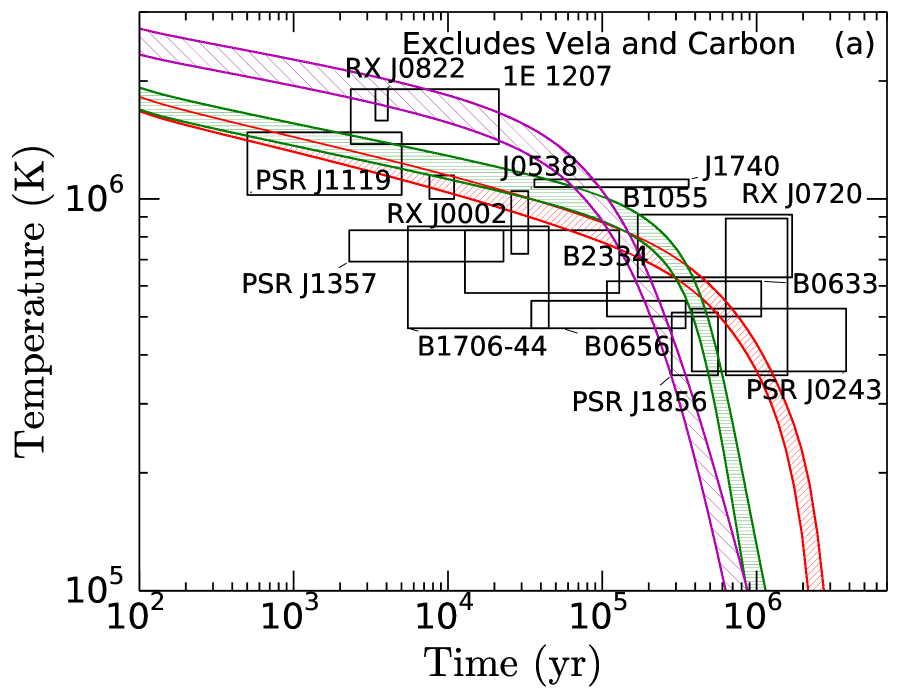
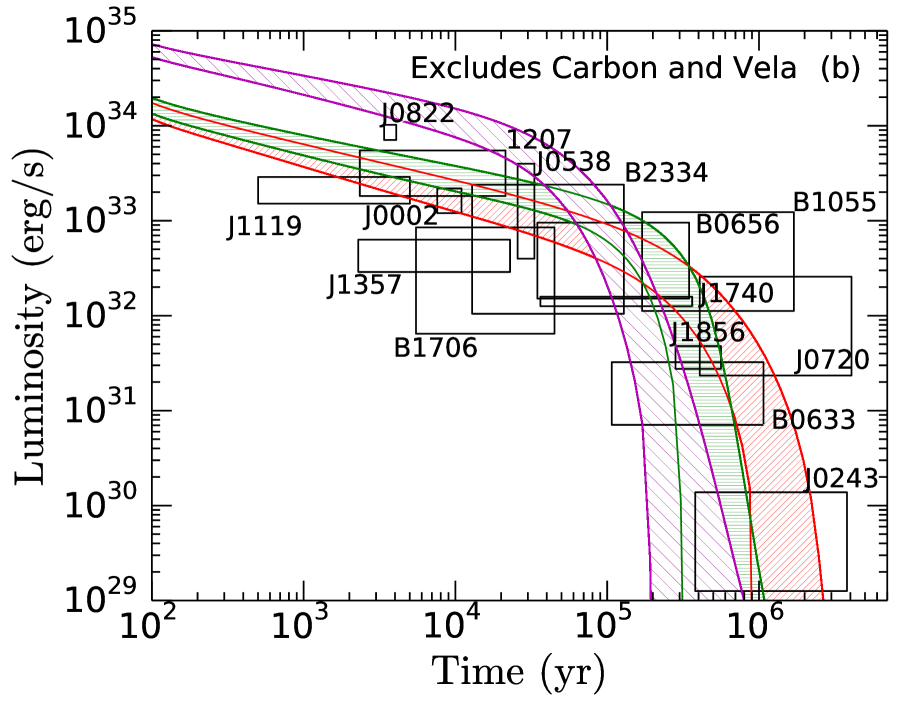
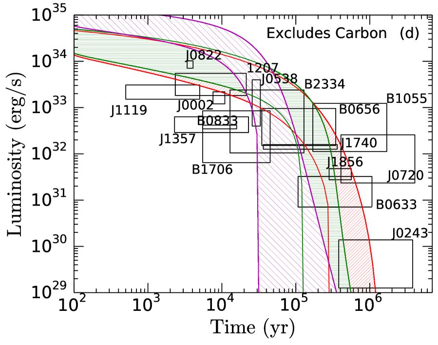
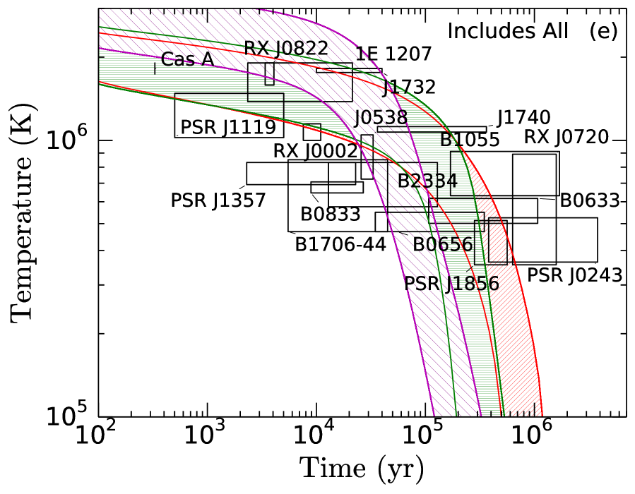
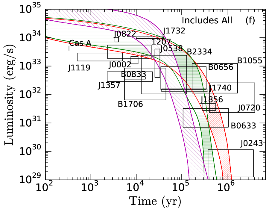
Figure 1: (Color online) Theoretical cooling curves illustrating how temperature and luminosity decrease over time. The black boxes represent neutron star cooling data and three colored bands show the $\pm 1\sigma$ uncertainties on the cooling curves (from superfluidity and superconductivity). The three bands represent three different values of $\eta$, $10^{-7}$ (purple, \\  hatching), $10^{-12}$ (green, horizontal hatching) and $10^{-17}$ (red, // hatching). The temperature results [labeled (a), (c), and (e)] correspond to the parameter limits in Table 2, while the luminosity results [labeled (b), (d), and (f)] correspond to the parameter limits in Table 3.

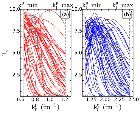
Figure 2: Uncorrelated samples from the critical temperatures from the fit to the luminosities as a function of the Fermi momenta for protons [left panel, (a)] and neutrons [right panel, (b)] without Vela or the carbon stars. The left boundary in both panels represents the Fermi momentum at the crust-core transition (denoted “$k^{\rm{p}}_{\rm{f}}\,\rm{min}$”). The right boundary represents the Fermi momentum in the center (denoted “$k^{\rm{n}}_{\rm{f}}\,\rm{max}$”) of a $1.4~{}\mathrm{M}_{\odot}$ neutron star. The uncertainty in the critical temperatures is large and there is a preference for proton superconductivity to peak at lower Fermi momenta.

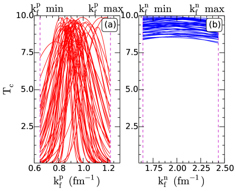
Figure 3: Uncorrelated samples from the critical temperatures from the fit to the luminosities as in Fig. 2 but now with Vela. Similar to previous works, we find strong proton superconductivity (a) and slightly weaker neutron triplet superfluidity (b). The proton superconductivity moves to higher densities and the density dependence of the neutron superfluid gap broadens to maximize the cooling to match the low luminosity of Vela.

Quantity	Value and 1$-\sigma$ uncertainty
	w/o Vela or carbon	w/o carbon	all
$\log_{10}T_{c,\mathrm{peak},n}$	$8.32\pm 0.49$	$9.34\pm 0.38$	$9.55\pm 0.29$
$k_{F,\mathrm{peak},n}~{}(\mathrm{fm}^{-1})$	$1.78\pm 0.16$	$1.95\pm 0.12$	$1.714\pm 0.087$
$\Delta k_{F,n}~{}(\mathrm{fm}^{-1})$	$0.28\pm 0.12$	$2.05\pm 0.11$	$1.744\pm 0.089$
$\log_{10}T_{c,\mathrm{peak},p}$	$8.88\pm 0.63$	$9.26\pm 0.46$	$8.48\pm 0.42$
$k_{F,\mathrm{peak},p}~{}(\mathrm{fm}^{-1})$	$0.641\pm 0.11$	$0.928\pm 0.07$	$0.99\pm 0.09$
$\Delta k_{F,p}~{}(\mathrm{fm}^{-1})$	$0.276\pm 0.12$	$0.115\pm 0.047$	$0.21\pm 0.085$
$\log_{10}\eta_{\mathrm{Cas\>A}}$			$-9.51\pm 0.70$
$\log_{10}\eta_{\mathrm{XMMU\>J1732}}$			$-9.03\pm 0.81$
$\log_{10}\eta_{\mathrm{PSR\>J1119}}$	$-14.39\pm 0.98$	$-16.41\pm 0.40$	$16.51\pm 0.61$
$\log_{10}\eta_{\mathrm{RXJ\>0822}}$	$-9.3\pm 1.1$	$-9.88\pm 0.52$	$-9.99\pm 0.64$
$\log_{10}\eta_{\mathrm{1E\>1207}}$	$-10.0\pm 1.1$	$-10.9\pm 0.52$	$-10.22\pm 0.76\$
$\log_{10}\eta_{\mathrm{PSR\>J1357}}$	$-9.15\pm 0.94$	$-9.31\pm 0.68$	$-9.87\pm 0.88$
$\log_{10}\eta_{\mathrm{RX\>J0002}}$	$-16.41\pm 0.80$	$-16.84\pm 0.39$	$-16.17\pm 0.55$
$\log_{10}\eta_{\mathrm{PSR\>B0833}}$		$-8.27\pm 0.38$	$-8.44\pm 0.53$
$\log_{10}\eta_{\mathrm{PSR\>B1706}}$	$-9.46\pm 1.1$	$-8.33\pm 0.52$	$-8.42\pm 0.50$
$\log_{10}\eta_{\mathrm{PSR\>J0538}}$	$-16.00\pm 0.10$	$-16.69\pm 0.57$	$-16.80\pm 0.46\hphantom{-1}$
$\log_{10}\eta_{\mathrm{PSR\>B2334}}$	$-8.46\pm 0.64$	$-8.03\pm 0.35$	$-7.88\pm 0.27$

Table 3: Luminosity fits of the same posterior parameter values.

III Results

We begin by removing Vela (PSR B0833$-$45) and the two carbon atmosphere stars in Cas A and XMMU J1732. We perform a MCMC simulation as described above, assuming that the minimal cooling model holds, i.e., that the direct Urca process does not operate and that no exotic matter is present. We fit the theoretical effective surface temperatures (accounting for the redshift factor) to the temperatures in Table 1 implied by the x-ray spectra. The resulting gap parameters, the envelope compositions, and their uncertainties (which we have assumed symmetric with respect to their central values) are given in the first column of Table 2. The posterior cooling curves for $\eta=0,10^{-12}$, and $10^{-7}$ are plotted in the top left panel of Fig. 1. We find large uncertainties in the critical temperatures for the singlet proton gap and the triplet neutron gap, and our numbers are not in disagreement with previous results from Ref. Page et al. (2009).

The results from fitting the luminosities rather than the temperatures are presented in the upper right panel of Fig. 1 and the first column of Table 3. The results are relatively similar to those obtained by fitting the temperature rather than the luminosity. Representative curves which show the dependence of the superfluid gaps on Fermi momentum are given in Fig. 2, showing that the proton superconducting gap is likely largest just near the crust core transition and falls off dramatically at the highest densities in the core. The triplet neutron superfluid critical temperature, on the other hand, may peak at any density so long as a large enough portion of the core undergoes the superfluid phase transition.

The quantitative nature of our fit also allows us to determine the envelope composition for H atmosphere neutron stars. We find PSR J1119-6127, RX J0002+6246 and PSR J0538+2817 all most likely have no light elements in their envelopes, in contrast with a small amount of light elements in 1E 1207.4-5209 and a significant contribution from light elements in all of the other H atmosphere stars. Note that stars which lie to the left and below the cooling curves tend to have a large amount of light elements, fitting better to the $\eta=10^{-7}$ (purple) curve lying to the right of the data point than the $\eta=10^{-17}$ (red) curve above the data point (because the time uncertainty is larger than the temperature uncertainty).

Now we add Vela and redo the temperature fit. The results are summarized in the second column of Table 2, and the middle left panel of Fig. 1. This one data point, lying to the left and below the curves, has a strong impact: The critical temperatures implied by the data are much larger than those obtained previously. We find neutron superfluid critical temperatures near $10^{9}$ K are required to explain the data and the width of the Gaussian increases significantly allowing a large part of the core to participate in the Cooper pair neutrino emissivity. The proton superconducting gap also increases slightly and moves to higher densities. The fit to the luminosities shown in the second column of Table 3 and the middle right panel in Fig. 1 shows the same trend. Representative curves which show the critical temperature are given in Fig. 3. The increase in gaps leads to a larger uncertainty in the cooling curves, as a larger part of the star now participates in the pair-breaking neutrino emissivity and thus the cooling is more sensitive to the gaps. The dramatic effect of Vela is partially because of the age revision of Vela down to $(5-16)\times 10^{3}$ years as obtained in Ref. Tsuruta et al. (2009) and discussed in Ref. Page et al. (2009). The envelope compositions are unchanged (within errors) and the fit prefers a significant amount of light elements in Vela’s envelope to become closer to the $\eta=10^{-7}$ curve lying to the right.

While the absolute normalization of the likelihood function is not meaningful, relative values are physical. A typical data point contributes a factor of 0.5 to the likelihood while Vela’s contribution is $10^{-3}$. This is a strong indication that fitting Vela is difficult in the minimal cooling model. The observation of Vela, as it currently stands, provides some evidence for the direct Urca process or the presence of exotic matter in neutron star cores.

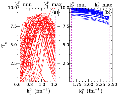
Figure 4: Uncorrelated samples from the critical temperatures from the fit to the luminosities as in Figs. 2 and 3 now having added both Vela (B0833$-$45) and the carbon-atmosphere stars to the analysis [(a) displays proton critical temperatures; (b) displays neutron critical temperatures]. Comparing to Fig. 3, the proton critical temperatures are smaller. The smaller proton critical temperature ensures younger stars are warm enough to match the relatively large luminosities from these two stars.

Previous works Page et al. (2011); Shternin et al. (2011) found very strong constraints on proton singlet superfluidity and neutron triplet superfluidity from observations which implied the neutron star in Cas A had cooled over a 10-year observation period Ho and Heinke (2009). References Blaschke et al. (2012, 2013) present an alternative explanation: In-medium effects on thermal conductivity as well as the presence of a particular proton gap explain the cooling. Reference Ho et al. (2015) found similar constraints on the gaps as found in Refs. Page et al. (2011); Shternin et al. (2011), and employed a polynomial parametrization of the gaps [in contrast to the Gaussian form we use in Eq.( 1)]. Recent observations of the neutron star in Cas A imply that it may not have cooled appreciably in the past 15 years Elshamouty et al. (2013); Posselt et al. (2013). For this work, we assume that the systematics do not enable us to constrain the cooling over a short time scale.

Employing this assumption, adding the neutron star in Cas A to the data set does not make a strong modification in our results. Because the surface temperature of Cas A lies in between the results for envelopes with and without light elements we simply choose a moderate amount of light elements $\eta\sim 10^{-10}$ to explain the data. However, adding the other neutron star thought to have a carbon atmosphere, XMMU J1732, creates a strong preference for warmer stars with light element envelopes. The results are summarized in the third column of Table 2 (for the temperature fit), and the third column of Table 3 (for the luminosity fit), and the bottom panels of Figs. 1 and  4. We find strong neutron superfluidity is required with a weak dependence on the neutron Fermi momenta and moderate proton superfluidity with a larger uncertainty on the proton Fermi momentum for which the critical temperature is maximized. These results are in strong tension with Vela, which has a strong preference for cooler stars with light element envelopes. This tension results in very tight constraints on the superfluid properties of dense matter. In the context of Bayesian inference where the evidence for a particular model is determined by the integral over the likelihood, the dramatic decrease in the parameter uncertainties leads to a model with very small evidence. In other words, if Vela and XMMU J1732 are confirmed to have ages and temperatures near the central values reported in Table 1, then it is likely that a model with some additional parameter which enables faster cooling in Vela will provide a much better fit.

IV Discussion

Most importantly, our work quantifies the extent to which superfluid properties can be constrained from currently available data on the cooling of isolated neutron stars. Most of the previous works on this topic give more qualitative results: They do not employ any particular likelihood function and thus cannot give full posteriors for their parameter values. The extent to which our quantitative approach will be possible without making the assumptions of the minimal cooling model will be explored in future work.

Our analysis has either 14, 15, or 17 parameters corresponding to 15, 16, or 18 data points, respectively. One of the advantages of our Bayesian approach is that our formalism does not require the fitting problem to be strongly over-constrained. Had we not employed the minimal cooling model, we would have required at least four new parameters to describe the EOS and an additional mass parameter for each neutron star (bringing us to a total of 39 parameters for 18 data points). An accurate mass measurement for even a few of the neutron stars in this data set would improve the fitting problem substantially.

One possible extension would be to attempt to explain the surface temperatures of accreting neutron stars as well, as done in Refs. Beznogov and Yakovlev (2015a) and Beznogov and Yakovlev (2015b). It is well known that some of those objects, in particular SAX J1808.4$-$3658, are too cold to be explained within the minimal cooling model Heinke et al. (2007), and thus the direct Urca process is invoked. The approach taken in Refs. Beznogov and Yakovlev (2015a) and Beznogov and Yakovlev (2015b) is similar in that they employ a systematic exploration of their parameter space; it is different in that they do not explicitly compute the likelihood of their models as we have done in Eq. (4). Extending our method to include the direct Urca process would necessitate also considering the variation in the EOS as well.

Our theoretical model presumes that the surface temperature of the neutron star does not vary across the surface. Hot spots on the neutron star surface may not create pulsations in the emission if they lie near the axis of rotation. It was argued that fits to the luminosity rather than the effective temperature partially ameliorate this difficulty because uneven temperature distributions impact the shape of the spectrum more strongly than the luminosity Potekhin et al. (2015). Our results demonstrate that the luminosity and temperature fits obtain qualitatively similar constraints on the superfluid gaps with some quantitative differences (for example, the luminosity fit implies different critical temperatures for proton superconductivity, especially when Vela is included). Nevertheless, fitting to luminosities rather than temperatures may be insufficient to fully explain the data if the temperature variation across the surface is dramatic.

Our model computes an effective surface temperature based on an atmosphere model and the amount of light elements in the envelope (see Ref. Potekhin (2014) for a recent review). The observed x-ray data is analyzed presuming a H atmosphere (sometimes including an estimate of the magnetic field), a carbon atmosphere, or a black body spectrum. Our results are thus limited by these two ingredients insofar as they allow us to correctly determine the temperature at the base of the envelope.

Several authors have examined the cooling of isolated neutron stars outside the minimal model. Reference Tsuruta et al. (2009) examined cooling with hyperons, and finds that superfluidity is required to ensure that the direct Urca process does not make neutron stars too cold. By allowing the direct Urca process, Refs. de Carvalho et al. (2015); Grigorian et al. (2015, 2016); Sedrakian (2016a) obtain a strong EOS dependence in their results. These works, along with Refs. Beznogov and Yakovlev (2015a, b), find that the data can be explained without exotic matter so long as the direct Urca process operates in some stars. We find (as first found in Ref. Page et al. (2004)), that the isolated neutron stars (with the exception of the Vela pulsar) can be easily explained without having to invoke the direct Urca process, so long as one allows for variations in the envelope composition at early times. Reference Sedrakian (2016b) has invoked axions in a model which does not include the direct Urca process. While we are performing our work in a model which contains more restrictive assumptions about the nature of dense matter, our statistical analysis allows us to be more quantitative in our conclusions. Extensions of this work beyond the minimal cooling model are in progress.

For the neutron stars with a carbon atmosphere, Ref. Ho et al. (2015) performs a $\chi^{2}$ fit to the data for the neutron star in Cas A, under the alternative assumption that this neutron star is indeed cooling quickly as found in Ref. Ho and Heinke (2009). A $\chi^{2}$ fit is possible here because there is no uncertainty in the $x$ axis, and thus the likelihood function in Eq. (4) gives the same result. We include a larger data set and perform our Monte Carlo over a much larger set of cooling models. Reference Noda et al. (2013) also assumes that Cas A is cooling quickly, and explains the data using a neutrino emissivity from superconducting quarks. The cooling of the carbon atmosphere star XMMU J1732 was addressed in Ref. Ofengeim et al. (2015), who also found a large heat blanketing envelope was required to reproduce the data. Reference Ofengeim et al. (2015) also obtained a constraint on the mass and radius of this neutron star because, in their model, the proton superfluid gap is correlated with the mass and radius. In contrast, we treat the EOS and superfluid properties of matter as independent. Ref. Suleimanov et al. (2017) has argued that the x-ray spectra of Cas A and XMMU J1732 can also be modeled as H atmospheres with hot spots as opposed to uniformly emitting carbon modeled surfaces. This possibility will be considered in future work.

We have presented results with and without Vela, the neutron star in Cas A, and XMMU J1732, but we cannot yet definitively determine whether or not those objects should be included or left out. The decrease in the fit quality may support going beyond the minimal model to explain Vela and an alternative interpretation for XMMU J1732 (such as that in Ref. Suleimanov et al. (2017)), but the final answer on this question requires more data or smaller uncertainties.

V Acknowledgements

The authors would like to thank Jim Lattimer and Madappa Prakash for useful discussions. S.B., S.H., and A.W.S. were supported by Grant No. NSF PHY 1554876. This work was supported by U.S. DOE Office of Nuclear Physics. This project used computational resources from the University of Tennessee and Oak Ridge National Laboratory’s Joint Institute for Computational Sciences.

References

- Lattimer and Prakash (2001) J. M. Lattimer and M. Prakash, Astrophys. J. 550, 426 (2001), URL http://dx.doi.org/10.1086/319702.
- Steiner et al. (2015) A. W. Steiner, S. Gandolfi, F. J. Fattoyev, and W. G. Newton, Phys. Rev. C 91, 015804 (2015), URL http://dx.doi.org/10.1103/PhysRevC.91.015804.
- Nättilä et al. (2016) J. Nättilä, A. W. Steiner, J. J. E. Kajava, V. F. Suleimanov, and J. Poutanen, Astron. Astrophys. 591, A25 (2016), URL http://dx.doi.org/10.1051/0004-6361/201527416.
- Ozel and Freire (2016) F. Ozel and P. Freire, Ann. Rev. Astron. Astrophys. 54, 401 (2016), URL http://dx.doi.org/10.1146/annurev-astro-081915-023322.
- Gandolfi et al. (2015) S. Gandolfi, A. Gezerlis, and J. Carlson, Ann. Rev. Nucl. Part. Sci. 65, 303 (2015), URL http://dx.doi.org/10.1146/annurev-nucl-102014-021957.
- Page et al. (2014) D. Page, J. M. Lattimer, M. Prakash, and A. W. Steiner, Stellar Superfluids (2014), chap. 21, ISBN 9780198719267, URL http://www.arxiv.org/abs/1302.6626.
- Page et al. (2004) D. Page, J. M. Lattimer, M. Prakash, and A. W. Steiner, Astrophys. J. Supp. 155, 623 (2004), URL http://dx.doi.org/10.1086/424844.
- Yakovlev and Pethick (2004) D. Yakovlev and C. Pethick, Annual Review of Astronomy and Astrophysics 42, 169 (2004), URL http://dx.doi.org/10.1146/annurev.astro.42.053102.134013.
- Page and Reddy (2006) D. Page and S. Reddy, Ann. Rev. Nucl. Part. Sci. 56, 327 (2006), URL http://dx.doi.org/10.1146/annurev.nucl.56.080805.140600.
- Steiner et al. (2016) A. W. Steiner, J. M. Lattimer, and E. F. Brown, Eur. Phys. J. A 52, 18 (2016), URL http://dx.doi.org/10.1140/epja/i2016-16018-1.
- Gudmundsson et al. (1983) E. H. Gudmundsson, C. J. Pethick, and R. I. Epstein, Astrophys. J. 272, 286 (1983), URL https://dx.doi.org/10.1086/161292.
- Potekhin et al. (1997) A. Y. Potekhin, G. Chabrier, and D. G. Yakovlev, Astron. Astrophys. 323, 415 (1997), URL http://aa.springer.de/papers/7323002/2300415.pdf.
- Potekhin (2014) A. Y. Potekhin, Phys. Usp. 57, 735 (2014), URL https://dx.doi.org/10.3367/UFNe.0184.201408a.0793.
- Page et al. (2009) D. Page, J. M. Lattimer, M. Prakash, and A. W. Steiner, Astrophys. J. 707, 1131 (2009), URL http://dx.doi.org10.1088/0004-637X/707/2/1131.
- Fesen et al. (2006) R. A. Fesen, M. C. Hammell, J. Morse, R. A. Chevalier, K. J. Borkowski, M. A. Dopita, C. L. Gerardy, S. S. Lawrence, J. C. Raymond, and S. van den Bergh, Astrophys. J. 645, 283 (2006), URL https://dx.doi.org/10.1086/504254.
- Ho and Heinke (2009) W. C. G. Ho and C. O. Heinke, Nature 462, 71 (2009), URL http://dx.doi.org/0.1038/nature08525.
- Kumar et al. (2012) H. S. Kumar, S. Safi-Harb, and M. E. Gonzalez, Astrophys. J. 754, 96 (2012), URL https://dx.doi.org/10.1088/0004-637X/754/2/96.
- Safi-Harb and Kumar (2008) S. Safi-Harb and H. S. Kumar, Astrophys. J. 684, 532-541 (2008), URL http://dx.doi.org/10.1086/590359.
- Zavlin et al. (1999) V. E. Zavlin, J. Trümper, and G. G. Pavlov, Astrophys. J. 525, 959 (1999), URL http://dx.doi.org/10.1086/307919.
- Zavlin et al. (2000) V. E. Zavlin, G. G. Pavlov, D. Sanwal, and J. Trümper, Astrophys. J. Lett. 540, L25 (2000), URL http://stacks.iop.org/1538-4357/540/i=1/a=L25.
- Roger et al. (1988) R. S. Roger, D. K. Milne, M. J. Kesteven, K. J. Wellington, and R. F. Haynes, Astrophys. J 332, 940 (1988), URL http://dx.doi.org/10.1086/166703.
- Pavlov et al. (2002) G. G. Pavlov, V. E. Zavlin, D. Sanwal, and J. Trumper, Astrophys. J. Lett. 569, 95 (2002), URL http://dx.doi.org/10.1086/340640.
- Mereghetti et al. (1996) S. Mereghetti, G. F. Bignami, and P. A. Caraveo, Astrophys. J. 464, 842 (1996), URL http://dx.doi.org/10.1086/177370.
- Zavlin et al. (1998) V. E. Zavlin, G. G. Pavlov, and J. Trumper, Astron. & Astrophys. 331, 821 (1998), URL http://arxiv.org/abs/astro-ph/9709267.
- Zavlin (2007a) V. E. Zavlin, Astrophys. J. Lett. 665, 143 (2007a), URL http://dx.doi.org/10.1086/521300.
- Pavlov et al. (2004) G. G. Pavlov, D. Sanwal, and M. A. Teter, IAU Symp. 218, 239 (2004), URL http://www.arxiv.org/abs/astro-ph/0311526.
- Tsuruta et al. (2009) S. Tsuruta, J. Sadino, A. Kobelski, M. A. Teter, A. C. Liebmann, T. Takatsuka, K. Nomoto, and H. Umeda, Astrophys. J. 691, 621 (2009), URL http://dx.doi.org/10.1088/0004-637X/691/1/621.
- Pavlov et al. (2001) G. G. Pavlov, V. E. Zavlin, D. Sanwal, V. Burwitz, and G. Garmire, Astrophys. J. Lett. 552, 129 (2001), URL http://dx.doi.org/10.1086/320342.
- Gotthelf et al. (2002) E. V. Gotthelf, J. P. Halpern, and R. Dodson, Astrophys. J. Lett. 567, 125 (2002), URL http://dx.doi.org/10.1086/340109.
- McGowan et al. (2004) K. E. McGowan, S. Zane, M. Cropper, J. A. Kennea, F. A. Cordova, C. Ho, T. Sasseen, and W. T. Vestrand, Astrophys. J. 600, 343 (2004), URL http://dx.doi.org/10.1086/379787.
- Tian et al. (2008) W. W. Tian, D. A. Leahy, M. Haverkorn, and B. Jiang, Astrophys. J. 679, L85 (2008), URL http://dx.doi.org/10.1086/589506.
- Klochkov et al. (2015) D. Klochkov, V. Suleimanov, G. Pühlhofer, D. G. Yakovlev, A. Santangelo, and K. Werner, Astron. Astrophys. 573, A53 (2015), URL http://dx.doi.org/10.1051/0004-6361/201424683.
- Kramer et al. (2003) M. Kramer, A. G. Lyne, G. Hobbs, O. Lohmer, P. Carr, C. Jordan, and A. Wolszczan, Astrophys. J. Lett. 593, 31 (2003), URL http://dx.doi.org10.1086/378082.
- Zavlin and Pavlov (2004) V. E. Zavlin and G. G. Pavlov, Mem. Soc. Ast. It. 75, 458 (2004), URL http://sait.oat.ts.astro.it/MmSAI/75/PDF/458.pdf.
- McGowan et al. (2003) K. E. McGowan, J. A. Kennea, S. Zane, F. A. Córdova, M. Cropper, C. Ho, T. Sasseen, and W. T. Vestrand, Astrophys. J. 591, 380 (2003), URL http://dx.doi.org/10.1086/375332.
- McGowan et al. (2006) K. E. McGowan, S. Zane, M. Cropper, W. T. Vestrand, and C. Ho, Astrophys. J. 639, 377 (2006), URL http://dx.doi.org/10.1086/497327.
- Zavlin (2007b) V. E. Zavlin, in Neutron Stars and Pulsars: About 40 Years After the Discovery (2007b), vol. 357, p. 181, URL http://dx.doi.org/10.1007/978-3-540-76965-1_9.
- Mignani et al. (2015) R. P. Mignani, P. Moran, A. Shearer, V. Testa, A. Sowikowska, B. Rudak, K. Krzeszowki, and G. Kanbach, Astron. Astrophys. 583, A105 (2015), eprint 1510.01057, URL http://dx.doi.org/10.1051/0004-6361/201527082.
- Possenti et al. (1996) A. Possenti, S. Mereghetti, and M. Colpi, Astron. Astrophys. 313, 565 (1996), URL http://adsabs.harvard.edu/abs/1996A%26A...313..565P.
- McLaughlin et al. (2002) M. A. McLaughlin, Z. Arzoumanian, J. M. Cordes, D. C. Backer, A. N. Lommen, D. R. Lorimer, and A. F. Zepka, Astrophys. J. 564, 333 (2002), URL https://dx.doi.org/10.1086/324151.
- Kargaltsev et al. (2012) O. Kargaltsev, M. Durant, Z. Misanovic, and G. Pavlov, Science 337, 946 (2012), URL https://dx.doi.org/10.1126/science.1221378.
- Viganò et al. (2013) D. Viganò, N. Rea, J. A. Pons, R. Perna, D. N. Aguilera, and J. A. Miralles, Mon. Not. R. Astron. Soc. 434, 123 (2013), URL https://dx.doi.org/10.1093/mnras/stt1008.
- Halpern and Wang (1997) J. P. Halpern and F. Y.-H. Wang, Astrophys. J. 477, 905 (1997), URL http://iopscience.iop.org/article/10.1086/303743/pdf.
- Ho (2007) W. C. G. Ho, Mon. Not. Roy. Astron. Soc. 380, 71 (2007), URL http://dx.doi.org/10.1111/j.1365-2966.2007.12043.x.
- Pons et al. (2002) J. A. Pons, F. M. Walter, J. M. Lattimer, M. Prakash, R. Neuhauser, and P.-h. An, Astrophys. J. 564, 981 (2002), URL http://dx.doi.org/10.1086/324296.
- Burwitz et al. (2003) V. Burwitz, F. Haberl, R. Neuhaeuser, P. Predehl, J. Truemper, and V. E. Zavlin, Astron. Astrophys. 399, 1109 (2003), URL http://dx.doi.org/10.1051/0004-6361:20021747.
- Pavlov and Zavlin (2003) G. G. Pavlov and V. E. Zavlin, in Proceedings 21st Texas Symposium on Relativistic Astrophysics. Edited by R. Bandiera, R. Maiolino and F. Mannucci. Singapore, World Scientific, 2003. p. 319 (2003), URL http://www.arxiv.org/abs/astro-ph/0305435.
- de Vries et al. (2004) C. P. de Vries, J. Vink, M. Mendez, and F. Verbunt, Astron. Astrophys. 415, L31 (2004), URL http://dx.doi.org/10.1051/0004-6361:20040009.
- Kaplan et al. (2002) D. L. Kaplan, S. R. Kulkarni, M. H. van Kerkwijk, and H. L. Marshall, Astrophys. J. Lett. 570, 79 (2002), URL http://dx.doi.org/10.1086/341102.
- Kaplan et al. (2003) D. L. Kaplan, M. H. van Kerkwijk, H. L. Marshall, B. A. Jacoby, S. R. Kulkarni, and D. A. Frail, Astrophys. J. 590, 1008 (2003), URL http://dx.doi.org/10.1086/375052.
- Lim et al. (2017) Y. Lim, C. H. Hyun, and C.-H. Lee, Int. J. Mod. Phys. E 26, 1750015 (2017), URL https://dx.doi.org/10.1142/S021830131750015X.
- Esposito et al. (2008) P. Esposito, A. De Luca, A. Tiengo, A. Paizis, S. Mereghetti, and P. A. Caraveo, Mon. Not. Roy. Astron. Soc. 384, 225 (2008), URL http://dx.doi.org/10.1111/j.1365-2966.2007.12677.x.
- Zavlin et al. (2004) V. E. Zavlin, G. G. Pavlov, and D. Sanwal, Astrophys. J. 606, 444 (2004), URL http://dx.doi.org/10.1086/382725.
- Akmal et al. (1998) A. Akmal, V. R. Pandharipande, and D. G. Ravenhall, Phys. Rev. C 58, 1804 (1998), URL http://dx.doi.org/10.1103/PhysRevC.58.1804.
- Flowers et al. (1976) E. Flowers, M. Ruderman, and P. Sutherland, Astrophys. J. 205, 541 (1976), URL http://dx.doi.org/10.1086/154308.
- Leinson and Perez (2006) L. B. Leinson and A. Perez, arXiv:astro-ph/0606653 (2006), URL http://arxiv.org/abs/astro-ph/0606653.
- Leinson and Pérez (2006) L. B. Leinson and A. Pérez, Phys. Lett. B 638, 114 (2006), URL http://dx.doi.org/10.1016/j.physletb.2006.05.036.
- Steiner and Reddy (2009) A. W. Steiner and S. Reddy, Phys. Rev. C 79, 015802 (2009), URL http://dx.doi.org/10.1103/PhysRevC.79.015802.
- Leinson (2010) L. B. Leinson, Phys. Rev. C 81, 025501 (2010), URL https://dx.doi.org/10.1103/PhysRevC.81.025501.
- Isobe et al. (1990) T. Isobe, E. D. Feigelson, M. G. Akritas, and G. J. Babu, Astrophys. J. 364, 104 (1990), URL http://dx.doi.org/10.1086/169390.
- Draper and Yang (1997) N. R. Draper and Y. Yang, Comp. Stat. and Data Anal. 23, 355 (1997), URL http://dx.doi.org/10.1016/S0167-9473(96)00037-0.
- Strömberg (1990) G. Strömberg, Astrophys. J. 92, 156 (1990), URL http://dx.doi.org/10.1086/144209.
- Steiner et al. (2010) A. W. Steiner, J. M. Lattimer, and E. F. Brown, Astrophys. J. 722, 33 (2010), URL http://dx.doi.org/10.1088/0004-637X/722/1/33.
- Page et al. (2011) D. Page, M. Prakash, J. M. Lattimer, and A. W. Steiner, Phys. Rev. Lett. 106, 081101 (2011), URL http://dx.doi.org/10.1103/PhysRevLett.106.081101.
- Shternin et al. (2011) P. S. Shternin, D. G. Yakovlev, C. O. Heinke, W. C. G. Ho, and D. J. Patnaude, Mon. Not. R. Astron. Soc. Lett. 412, 108 (2011), URL http://dx.doi.org/10.1111/j.1745-3933.2011.01015.x.
- Blaschke et al. (2012) D. Blaschke, H. Grigorian, D. N. Voskresensky, and F. Weber, Phys. Rev. C 85, 022802 (2012), URL http://dx.doi.org/10.1103/PhysRevC.85.022802.
- Blaschke et al. (2013) D. Blaschke, H. Grigorian, and D. N. Voskresensky, Phys. Rev. C 88, 065805 (2013), URL http://dx.doi.org/10.1103/PhysRevC.88.065805.
- Ho et al. (2015) W. C. G. Ho, K. G. Elshamouty, C. O. Heinke, and A. Y. Potekhin, Phys. Rev. C 91, 015806 (2015), URL http://dx.doi.org/10.1103/PhysRevC.91.015806.
- Elshamouty et al. (2013) K. G. Elshamouty, C. O. Heinke, G. R. Sivakoff, W. C. G. Ho, P. S. Shternin, D. G. Yakovlev, D. J. Patnaude, and L. David, Astrophys. J. 777, 22 (2013), URL http://dx.doi.org/10.1088/0004-637X/777/1/22.
- Posselt et al. (2013) B. Posselt, G. G. Pavlov, V. Suleimanov, and O. Kargaltsev, Astrophys. J. 779, 186 (2013), URL http://dx.doi.org/10.1088/0004-637X/779/2/186.
- Beznogov and Yakovlev (2015a) M. V. Beznogov and D. G. Yakovlev, Mon. Not. Roy. Astron. Soc. 447, 1598 (2015a), URL http://dx.doi.org/10.1093/mnras/stu2506.
- Beznogov and Yakovlev (2015b) M. V. Beznogov and D. G. Yakovlev, Mon. Not. Roy. Astron. Soc. 452, 540 (2015b), URL http://dx.doi.org/10.1093/mnras/stv1293.
- Heinke et al. (2007) C. O. Heinke, P. G. Jonker, R. Wijnands, and R. E. Taam, Astrophys. J. 660, 1424 (2007), URL http://dx.doi.org/10.1086/513140.
- Potekhin et al. (2015) A. Y. Potekhin, J. A. Pons, and D. Page, Space Sci. Rev. 191, 239 (2015), URL https://dx.doi.org/10.1007/s11214-015-0180-9.
- de Carvalho et al. (2015) S. M. de Carvalho, R. Negreiros, M. Orsaria, G. A. Contrera, F. Weber, and W. Spinella, Phys. Rev. C 92, 035810 (2015), URL http://dx.doi.org/10.1103/PhysRevC.92.035810.
- Grigorian et al. (2015) H. Grigorian, D. Blaschke, and D. N. Voskresensky, Phys. Part. Nucl. 46, 849 (2015), URL http://dx.doi.org/10.1134/S1063779615050111.
- Grigorian et al. (2016) H. Grigorian, D. N. Voskresensky, and D. Blaschke, Eur. Phys. J. A 52, 67 (2016), URL http://dx.doi.org/10.1140/epja/i2016-16067-4.
- Sedrakian (2016a) A. Sedrakian, Eur. Phys. J. A 52, 44 (2016a), URL http://dx.doi.org/10.1140/epja/i2016-16044-y.
- Sedrakian (2016b) A. Sedrakian, Phys. Rev. D 93, 065044 (2016b), URL http://dx.doi.org/10.1103/PhysRevD.93.065044.
- Noda et al. (2013) T. Noda, M.-A. Hashimoto, N. Yasutake, T. Maruyama, T. Tatsumi, and M. Fujimoto, Astrophys. J. 765, 1 (2013), URL http://dx.doi.org/10.1088/0004-637X/765/1/1.
- Ofengeim et al. (2015) D. D. Ofengeim, A. D. Kaminker, D. Klochkov, V. Suleimanov, and D. G. Yakovlev, Mon. Not. R. Astroc. Soc. 454, 2668 (2015), URL http://dx.doi.org/10.1093/mnras/stv2204.
- Suleimanov et al. (2017) V. F. Suleimanov, D. Klochkov, J. Poutanen, and K. Werner, Astron. Astrophys. 600, A43 (2017), URL https://dx.doi.org/10.1051/0004-6361/201630028.