Learning physical descriptors for materials science
by compressed sensing

Abstract

The availability of big data in materials science offers new routes for analyzing materials properties and functions and achieving scientific understanding. Finding structure in these data that is not directly visible by standard tools and exploitation of the scientific information requires new and dedicated methodology based on approaches from statistical learning, compressed sensing, and other recent methods from applied mathematics, computer science, statistics, signal processing, and information science. In this paper, we explain and demonstrate a compressed-sensing based methodology for feature selection, specifically for discovering physical descriptors, i.e., physical parameters that describe the material and its properties of interest, and associated equations that explicitly and quantitatively describe those relevant properties. As showcase application and proof of concept, we describe how to build a physical model for the quantitative prediction of the crystal structure of binary compound semiconductors.

I Introduction

Big-data-driven research offers new routes towards scientific insight. This big-data challenge is not only about storing and processing huge amounts of data, but also, and in particular, it is a chance for new methodology for modeling, describing, and understanding. Let us explain this by a simple, but most influential, historic example. About 150 years ago, D. Mendeleev and others organized the 56 atoms that were known at their time in terms of a table, according to their weight and chemical properties. Many atoms were not yet identified, but from the table, it was clear that they should exist, and even their chemical properties were anticipated. The scientific reason behind the table, i.e., the shell structure of the electrons, was unclear and was understood only 50 years later when quantum mechanics had been developed. Finding structure in the huge space of materials, e.g., one table (or a map) for each property, or function of interest, is one of the great dreams of (big-)data-driven materials science.

Obviously, the challenge to sort all materials is much bigger than that of the mentioned example of the Periodic Table of Elements (PTE). Up to date, the PTE contains 118 elements that have been observed. About $200\,000$ materials are “known” to exist LB , but only for very few of these “known” materials, the basic properties (elastic constants, plasticity, piezoelectric tensors, thermal and electrical conductivity, etc.) have been determined. When considering surfaces, interfaces, nanostructures, organic materials, and hybrids of these mentioned systems, the amount of possible materials is practically infinite. It is, therefore, highly likely that new materials with superior and up to now simply unknown characterstics exist that could help solving fundamental issues in the fields of energy, mobility, safety, information, and health.

For materials science it is already clear that big data are structured, and in terms of materials properties and functions, the space of all possible materials is sparsely populated. Finding this structure in the big data, e.g., asking for efficient catalysts for CO₂ activation or oxidative coupling of methane, good thermal barrier coatings, shape memory alloys as artery stents, or thermoelectric materials for energy harvesting from temperature gradients, just to name a few examples, may be possible, even if the actuating physical mechanisms of these properties and functions are not yet understood in detail. Novel big-data analytics tools, e.g., based on machine learning or compressed sensing, promise to do so.

Machine learning of big data has been used extensively in a variety of fields ranging from biophysics and drug design to social media and text mining. It is typically considered a universal approach for ‘learning’ (fitting) a complex relationship $y=f(x)$. Some, though few, machine-learning based works have been done in materials science, e.g., Refs. Lorenz et al., 2004; Hautier et al., 2010; Behler, 2011; Pilania et al., 2013; Szlachta et al., 2014; Mueller et al., 2014; Schütt et al., 2014; Atsuto et al., 2015; Faber et al., 2015; Caccin et al., 2015; Isayev et al., 2015; Mannodi-Kanakkithodi et al., 2016; Kim et al., 2016; Ueno et al., 2016; Solovyeva and von Lilienfeld, 2016; Bialon et al., 2016. Most of them use kernel ridge regression or Gaussian processes, where in both cases the fitted/learned property is expressed as a weighted sum over all or selected data points. A clear breakthrough, demonstrating a ‘game change’, is missing, so far, and a key problem, emphasized in Ref. Ghiringhelli et al., 2015, is that a good feature selection for descriptor identification is central to achieving a good-quality, predictive statistically learned equation.

One of the purposes of discovering structure in materials-science data, is to predict a property of interest for a given complete class of materials. In order to do this, a model needs to be built, that maps some accessible, descriptive input quantities, identifying a material, into the property of interest. In statistical learning, this set of input parameters is called descriptor Ghiringhelli et al. (2015). For our materials science study, this descriptor (elsewhere also termed “fingerprint” Pilania et al. (2013); Isayev et al. (2015)) is a set of physical parameters that uniquely describe the material and its function of interest. It is important that materials that are very different (similar) with respect to the property or properties of interest, should be characterized by very different (similar) values of the descriptors. Moreover, the determination of the descriptor must not involve calculations as intensive as those needed for the evaluation of the property to be predicted.

In most papers published so far, the descriptor has been introduced ad hoc, i.e., without performing an extensive, systematic analysis and without demonstrating that it is the best (in some sense) within a certain broad class. The risk of such ad hoc approach is that the learning step is inefficient (i.e., very many data points are needed), the governing physical mechanisms remain hidden, and the reliability of predictions is unclear. Indeed, machine learning is understood as an interpolation and not extrapolation approach, and it will do so well, if enough data are available. However, quantum mechanics and materials science are so multifaceted and intricate that we are convinced that we hardly ever will have enough data. Thus, it is crucial to develop these tools as domain-specific methods and to introduce some scientific understanding, keeping the bias as low as possible.

In this paper, we present a methodology for discovering physically meaningful descriptors and for predicting physically (materials-science) relevant properties. The paper is organized as follows: In section II, we introduce compressed-sensingDonoho (2006); Candès and Wakin (2008); Davenport et al. (2012); Boche et al. (2015) based methods for feature selection; in section III, we introduce efficient algorithms for the construction and screening of feature spaces in order to single out “the best” descriptor. “Feature selection” is a widespread set of techniques that are used in statistical analysis in different fields Guyon and Elisseeff (2003). In the following sections, we analyze the significance of the descriptors found by the statistical-learning methods, by discussing the interpolation ability of the model based on the found descriptors (section IV), the stability of the models in terms of sensitivity analysis (section V), and the extrapolation capability, i.e., the possibility of predicting new materials (section VI).

As showcase application and proof of concept, we use the quantitative prediction of the crystal structure of binary compound semiconductors, which are known to crystallize in zincblende (ZB), wurtzite (WZ), or rocksalt (RS) structures. The structures and energies of ZB and WZ are very close and for the sake of clarity we will not distinguish them here. For many materials, the energy difference between ZB and RS is larger, though still very small, namely just 0.001% or less of the total energy of a single atom. Thus, high accuracy is required to predict this difference. The property $P$ that we aim to predict is the difference in the energies between RS and ZB for the given AB-compound material, $\Delta E_{\textrm{AB}}$. The energies are calculated within the Kohn-Sham formulationKohn and Sham (1965) of density-functional theory Hohenberg and Kohn (1964), with the local-density approximation (LDA) exchange-correlation functional Ceperley and Alder (1980); Perdew and Wang (1992). Since in this paper we are concerned with the development of a data-analytics approach, it is not relevant that also approximations better than LDA exist, only the internal consistency and the realistic complexity of the data are important. The below described methodology applies to these better approximations as well.

Clearly, the sign of $\Delta E_{\textrm{AB}}$ gives the classification (negative for RS and positive for ZB), but the quantitative prediction of $\Delta E_{\textrm{AB}}$ values gives a better understanding. The separation of RS and ZB structures into distinct classes, on the basis of their chemical formula only, is difficult and has existed as a key problem in materials science for over 50 years van Vechten (1969); Phillips (1970); Bloch and Simons (1972); John and Bloch (1974); Zunger (1980); Chelikowsky (1982); Pettifor (1984); Villars (1985); Andreoni et al. (1985); Andreoni and Galli (1987); Saad et al. (2012). In the rest of the paper, we will always write the symbol $\Delta E$, without the subscript AB, to signify the energy of the RS compound minus the energy of the ZB compound.

II Compressed-sensing based methods for feature selection

Let us assume that we are given data points $\{\bm{d}_{1},P_{1}\},\dots,\{\bm{d}_{N},P_{N}\}$, with $\bm{d}_{1},\dots,\bm{d}_{N}\in\mathbb{R}^{M}$ and $P_{1},\dots,P_{N}\in\mathbb{R}.$ We would like to analyze and understand the dependence of the output $P$ (for “Property”) on the input $\bm{d}$ (for “descriptor”), that reflects the specific measurement or calculation. Specifically, we are seeking for an interpretable equation $P=f(\bm{d})$, e.g., an explicit analytical formula, where $P$ depends on a small number of input parameters, i.e., the dimension of the input vector $\bm{d}$ is small. Below, we will impose constraints in order to arrive at a method for finding a low-dimensional linear solution for $P=f(\bm{d})$. Later, we introduce nonlinear transformations of the vector $\bm{d}$; dealing with such nonlinearities is the main focus of this paper.

When looking for a linear dependence $P=f(\bm{d})=\bm{d}\cdot\bm{c}$, the most simple approach to the problem is the method of least squares. This is the solution of

$$\mathop{\rm argmin}\limits_{\bm{c}\in\mathbb{R}^{M}}\sum_{j=1}^{N}\Bigl{(}P_{j}-\sum_{k=1}^{M}d_{j,k}c_{k}\Bigr{)}^{2}=\mathop{\rm argmin}\limits_{\bm{c}\in\mathbb{R}^{M}}\|\bm{P}-\bm{D}\bm{c}\|_{2}^{2},$$ (1)

where $\bm{P}=(P_{1},\dots,P_{N})^{T}$ is the column vector of the outputs and $\bm{D}=(d_{j,k})$ is the $(N\times M)$-dimensional matrix of the inputs, and the column vector $\bm{c}$ is to be determined. The equality defines the $\ell_{2}$ or Euclidean norm ($\|\cdot\|_{2}$) of the vector $\bm{P}-\bm{D}\bm{c}$. The resulting function would then be just the linear relationship $f(\bm{d})=\langle\bm{d},\bm{c}\rangle=\sum_{k=1}^{M}d_{k}c_{k}$. It is the function that minimizes the error $\|\bm{P}-\bm{D}\bm{c}\|_{2}^{2}$ among all linear functions of $\bm{d}$. Let us point out a few properties of Eq. (1). First, the solution of Eq. (1) is given by an explicit formula $\bm{c}=(\bm{D}^{T}\bm{D})^{-1}\bm{D}^{T}\bm{P}$ if $\bm{D}^{T}\bm{D}$ is a non-singular matrix. Second, it is a convex problem, therefore the solution could also be found efficiently even in large dimensions (i.e. if $M$ and $N$ are large) and there are many solvers available Bertsekas (1999). Finally, it does not put any more constraints on $\bm{c}$ (or $f$) than that it is linear and minimizes Eq. (1).

A general linear function $f$ of $\bm{d}$ usually involves also an absolute term, i.e. it has a form $f(\bm{d})=c_{0}+\sum_{k=1}^{M}d_{k}c_{k}$. It is easy to add the absolute term (also called bias) to Eq. (1) in the form

$$\mathop{\rm argmin}\limits_{c_{0}\in\mathbb{R},\bm{c}\in\mathbb{R}^{M}}\sum_{j=1}^{N}\Bigl{(}P_{j}-c_{0}-\sum_{k=1}^{M}d_{j,k}c_{k}\Bigr{)}^{2}.$$ (2)

This actually coincides with Eq. (1) if we first enlarge the matrix $\bm{D}$ by adding a column full of ones. We will tacitly assume in the following that this modification was included in the implementation and shall not repeat that any more.

If pre-knowledge is available, it can be (under some conditions) incorporated into Eq. (1). For example, we might want to prefer those vectors $\bm{c}$, which are small (in some sense). This gives rise to regularized problems. In particular, the ridge regression

$$\mathop{\rm argmin}\limits_{\bm{c}\in\mathbb{R}^{M}}\left(\|\bm{P}-\bm{D}\bm{c}\|_{2}^{2}+\lambda\|\bm{c}\|^{2}_{2}\right)$$ (3)

with a penalty parameter $\lambda>0$ weights the magnitude of the vector $\bm{c}$ and of the error of the fit against each other. The larger $\lambda$, the smaller is the minimizing vector $\bm{c}$. The smaller $\lambda$, the better is the least square fit (the first addend in Eq. (3)). More specifically, if $\lambda\to 0$, the solutions of Eq. (3) converge to the solution of Eq. (1). And if $\lambda\to\infty$, the solutions of Eq. (3) tend to zero.

II.1 Sparsity, NP-hard problems, and convexity of the minimization problem

The kind of pre-knowledge, which we will discuss next, is that we would like $f(\bm{d})$ depend only on a small number of components of $\bm{d}$. In the notation of Eq. (1), we would like to achieve that most of the components of the solution $\bm{c}$ are zero. Therefore, we denote the number of non-zero coordinates of a vector $\bm{c}$ by

$$\|\bm{c}\|_{0}=\#\{j:c_{j}\not=0\}.$$ (4)

Here, $\{j:c_{j}\not=0\}$ stands for the set of all the coordinates $j$, such that $c_{j}$ is non-zero, and $\#\{\ldots\}$ denotes the number of elements of the set $\{\ldots\}$. Thus, $\|\bm{c}\|_{0}$ is the number of non-zero elements of the vector $\bm{c}$, and it is often called the $\ell_{0}$ norm of $\bm{c}$. We say that $\bm{c}\in\mathbb{R}^{M}$ is $k$-sparse, if $\|\bm{c}\|_{0}\leq k$, i.e. if at most $k$ of its coordinates are not equal to zero.

When trying to regularize Eq. (1) in such a way that it prefers sparse solutions $\bm{c}$, one has to minimize:

$$\mathop{\rm argmin}\limits_{\bm{c}\in\mathbb{R}^{M}}\left(\|\bm{P}-\bm{D}\bm{c}\|_{2}^{2}+\lambda\|\bm{c}\|_{0}\right).$$ (5)

This is a rigorous formulation of the problem that we want to solve, but it has a significant drawback: It is computationally infeasible when $M$ is large. This can be easily understood as follows. The naive way of solving Eq. (5) is to look first on all index sets $T\subset\{1,\dots,M\}$ with one element and try to minimize over vectors supported in such sets. Then one looks for all subsets with two, three, and more elements. Unfortunately. their number grows quickly with $M$ and the level of sparsity $k$. It turns out, that this naive way can not be improved much. The problem is called “NP-hard”Arora and Barak (2009). In a “Non-deterministic Polynomial-time hard” problem, a good candidate for the solution can be checked in a polynomial time, but the solution itself can not be found in polynomial time. The basic reason is that Eq. (5) is not convex.

II.2 Methods based on the $\ell_{1}$ norm

Reaching a compromise between convexity and promoting sparsity is made possible by the LASSO (Least Absolute Shrinkage and Selection Operator)Tibshirani (1996) approach, in which the $\ell_{0}$ regularization of Eq. (5) is replaced by the $\ell_{1}$ norm:

$$\mathop{\rm argmin}\limits_{\bm{c}\in\mathbb{R}^{M}}\|\bm{P}-\bm{D}\bm{c}\|_{2}^{2}+\lambda\|\bm{c}\|_{1}.$$ (6)

The use of the $\ell_{1}$ norm ($\|\bm{c}\|_{1}=\sum_{k}|c_{k}|$), also known as the “Manhattan” or “Taxicab” norm, is crucial here. On the one hand, the optimization problem is convex Hastie et al. (2009). On the other hand, the geometry of the $\ell_{1}$-unit ball $\{\bm{x}\in\mathbb{R}^{M}:\|\bm{x}\|_{1}\leq 1\}$ shows, that it promotes sparsity Davenport et al. (2012); Boche et al. (2015).

Similarly to Eq. (3), the larger the $\lambda>0$, the smaller the $\ell_{1}$-norm of the solution of Eq. (6) would be, and vice versa. Actually, there exists a smallest $\lambda_{0}>0$, such that the solution of Eq. (6) is zero. If $\lambda$ then falls below this threshold, one or more components of $\bm{c}$ become non-zero.

II.3 Compressed sensing

The minimization problem in Eq. (6) is an approximation of the problem in Eq. (5), and their respective results do not necessarily coincide. The relation between these two minimization problems was studied intensively Greenshtein (2006); van de Geer (2008); Bühlmann and van de Geer (2011) and we summarize the results, developed in the context of a recent theory of compressed sensing (CS) Donoho (2006); Davenport et al. (2012); Boche et al. (2015). These will be useful for justifying the implementation of our method (see below). The literature on CS is extensive and we believe that the following notes are a useful compendium.

We are especially interested in conditions on $\bm{P}$ and $\bm{D}$ which guarantee that the solutions of Eqs. (5) and (6) coincide, or at least do not differ much. We concentrate on a simplified setting, namely attempting to find $\bm{c}\in\mathbb{R}^{M}$ fulfilling $\bm{Dc}=\bm{P}$ with fewest non-zero entries. This is written as

$$\mathop{\rm argmin}\limits_{\bm{c}:\bm{D}\bm{c}=\bm{P}}\|\bm{c}\|_{0}.$$ (7)

As mentioned above, this minimization is computationally infeasible, and we are interested in finding the same solution by its convex reformulation:

$$\mathop{\rm argmin}\limits_{\bm{c}:\bm{D}\bm{c}=\bm{P}}\|\bm{c}\|_{1}.$$ (8)

The answer can be characterized by the notion of the Null Space Property (NSP) Cohen et al. (2009). Let $\bm{D}\in\mathbb{R}^{M\times N}$ and let $\Omega\in\{1,\dots,N\}$. Then $\bm{D}$ is said to have the NSP of order $\Omega$ if

$$\sum_{j\in T}|v_{j}|<\sum_{j\not\in T}|v_{j}|\quad\forall\bm{v}\not=0\ \text{with}\ \bm{D}\bm{v}=0\ \forall T\subset\{1,\dots,N\}\ \text{with}\ \#T\leq\Omega.$$ (9)

It is shown Cohen et al. (2009) that every $\Omega$-sparse vector $\bm{x}$ is the unique solution of Eq. (8) with $\bm{P}=\bm{D}\bm{x}$ if, and only if, $\bm{D}$ has the NSP of order $\Omega$. As a consequence, the minimization of the $\ell_{1}$ norm as given by Eq. (8) recovers the unknown $\Omega$-sparse vectors ${\bm{c}}\in\mathbb{R}^{N}$ from $\bm{D}$ and $\bm{P}=\bm{D}\bm{c}$ only if $\bm{D}$ satisfies the NSP of order $\Omega$. Unfortunately, when given a specific matrix $\bm{D}$, it is not easy to check if it indeed has the NSP.

However, the CS analysis gives us some guidance for the admissible dimension $M$ of $\bm{D}.$ It is known Cohen et al. (2009); Boche et al. (2015) that there exists a constant $C>0$ such that whenever

$$M\geq C\ \!\Omega\ \!\ln(N)$$ (10)

then there exist matrices $\bm{D}\in\mathbb{R}^{M\times N}$ with NSP of order $\Omega$. Actually, a random matrix with these dimensions satisfies the NSP of order $\Omega$ with high probability. On the other hand, this bound is tight, i.e., if $M$ falls below this bound no stable and robust recovery of $\bm{c}$ from $\bm{D}$ and $\bm{P}$ is possible, and this is true for every matrix $\bm{D}\in\mathbb{R}^{M\times N}.$ Later on, $M$ will correspond to the number of AB compounds considered and will be fixed to $M=82$. Furthermore, $N$ will be the number of input features, and Eq. (10) tells us that we can expect reasonable performance of $\ell_{1}$-minimization only if their number is at most of the order $e^{\frac{M}{C\Omega}}.$

Furthermore, the CS analysis sets forth that the NSP is surely violated already for $\Omega=2$ if any two columns of $\bm{D}$ are a multiple of each other. In general, one can expect the solution of Eq. (8) to differ significantly from the solution of Eq. (7) if any two columns of $\bm{D}$ are highly correlated or, in general, if any of the columns of $\bm{D}$ lies close to the span of a small number of any other its columns.

Historically, LASSO appeared first in 1996 as a machine-learning (ML) technique, able to provide stable solutions to underdetermined linear systems, thanks to the $\ell_{1}$ regularization. Ten years later, the CS theory appeared, sharing with LASSO the concept of $\ell_{1}$ regularization, but the emphasis is on the reconstruction of a possibly noisy signal $\bm{c}$ from a minimal number of observations. CS can be considered the theory of LASSO, in the sense that it gives conditions (on the matrix $\bm{D}$) on when it is reasonable to expect that the $\ell_{1}$ and $\ell_{0}$ regularizations coincide. If the data and a, typically overcomplete, basis set are known, then LASSO is applied as a ML technique, where the task is to identify the smallest number of basis vectors that yield a model of a given accuracy. If the setting is such that a minimal set of measurements should be performed to reconstruct a signal, as in quantum-state tomography Gross et al. (2010), then CS tells how the data should be acquired. As it will become clear in the following, our situation is somewhat intermediate, in the sense that we have the data (here, the energy of the 82 materials), but we have a certain freedom to select the basis set for the model. Therefore, we use CS to justify the construction of the matrix $\bm{D}$, and we adopt LASSO as a mean to find the low-dimensional basis set.

II.4 A simple LASSO example: the energy differences of crystal structures

In this and following sections, we walk through the application of LASSO to a specific materials-science problem, in order to introduce step by step a systematic approach for finding simple analytical formulas, that are built from simple input parameters (the primary features), for approximating physical properties of interest. We aim at predicting $\Delta E_{\textrm{AB}}$, the difference in DFT-LDA energy between ZB and RS structures in a set of 82 octet binary semiconductors. Calculations were performed using the all-electron full-potential code FHI-aims Blum et al. (2009) with highly accurate basis sets, $\bf k$-meshes, integration grids, and scaled ZORA van Lenthe et al. (1994) for the relativistic treatment.

The order of the two atoms in the chemical formula AB is chosen such that element A is the cation, i.e., it has the smallest Mulliken electronegativity, $\textrm{EN}\!=\!-(\textrm{IP}+\textrm{EA})/2$. IP and EA are the ionization potential and electron affinity of the free, isolated, spinless, and spherical symmetric atom. As noted, the calculation of the descriptor must involve less intensive calculations than those needed for the evaluation of the property to be predicted. Therefore, we consider only properties of the free atoms A and B, that build the binary material, and properties of the gas-phase dimers. In practice, we identified the following primary features, exemplified for atom A: the ionization potential IP(A), the electron affinity EA(A) IPE , H(A) and L(A), i.e., the energies of the highest-occupied and lowest-unoccupied Kohn-Sham (KS) levels, and $r_{s}$(A), $r_{p}$(A), and $r_{d}$(A), i.e., the radii where the radial probability density of the valence $s$, $p$, and $d$ orbitals are maximal. The same features were used for atom B. Clearly, these primary features were chosen because it is well known since long that the relative ionization potentials, the atomic radii, and $sp$-hybridization govern the bonding in these materials. Consequently, some authorsSimons and Bloch (1973); Chelikowsky and Phillips (1978); Andreoni et al. (1979) already recognized that certain combinations of $r_{s}$ and $r_{p}$ – called $r_{\sigma}$ and $r_{\pi}$ (see below) – may be crucial for constructing a descriptor that predicts the RS/ZB classification. Note that just the sign of $\Delta E$ was predicted, while the model we present here targets at a quantitative prediction of $\Delta E$. In contrast to previous work, we analyze how LASSO will perform in this task and how much better the corresponding description is. We should also note that the selected set of atomic primary features contains redundant physical information, namely H(A) and L(A) contain similar information as IP(A) and EA(A). In particular H(A) $-$ L(A) is correlated, on physical grounds, to IP(A) $-$ EA(A). However, since the values of these two differences are not the same IPE , all four features were included. As it will be shown below and in particular in Appendix A, the two pairs of features are not interchangeable.

We start with a simplified example, in order to show in an easily reproducible way the performance of LASSO in solving our problem. To this extent, we describe each compound AB by the vector of the following six quantities:

$$\bm{d}_{\textrm{AB}}=(r_{s}(\textrm{A}),r_{p}(\textrm{A}),r_{d}(\textrm{A}),r_{s}(\textrm{B}),r_{p}(\textrm{B}),r_{d}(\textrm{B})).$$ (11)

All this data collected gives a $82\times 6$ matrix $\bm{D}$ – one row for each compound. We standardize $\bm{D}$ to have zero mean and variance 1, i.e. subtract from each column its mean and divide by its standard deviation. Standardization of the data is common practiceHastie et al. (2009) and aimed at controlling the numerical stability of the solution. However, when non-linear combinations of the features and cross-validation is involved, the standardization has to be performed carefully (see below). The energy differences are stored in a vector $\bm{P}\in\mathbb{R}^{82}.$

We are aiming at two goals:

• On the one hand, we would like to minimize the mean-squared error (MSE), a measure of the quality of the approximation, given by

  $$\frac{1}{N}\sum_{j=1}^{N}\Bigl{(}P_{j}-\sum_{k=1}^{M}d_{j,k}c_{k}\Bigr{)}^{2}.$$ (12)

  In this tutorial example, the size $N$ of the dataset is 82 and, with the above choice of Eq. (11), $M=6$.

• On the other hand, we prefer sparse solutions $\bm{c}^{\dagger}$ with small $\Omega$, as we like to explain the dependence of the energy difference $\bm{P}$ based on a low-dimensional (small $\Omega$) descriptor $\bm{d}^{\dagger}$.

These two tasks are obviously closely connected, and go against each other. The larger the coefficient $\lambda$ in Eq. (6), the more sparse the solution $\bm{c}$ will be; the smaller $\lambda$, the smaller the mean-squared error will be. The choice of $\lambda$ is at our disposal and let us weight sparsity of $\bm{c}$ against the size of the MSE.

In the following, we will rather report the root mean square error(RMSE) as a quality measure of a model. The reason is that the RMSE has the same units as the predicted quantities, therefore easier to understand in absolute terms. Specifically, when a sparse solution $\bm{c}^{\dagger}$ of Eq. (6) is mentioned, with $\Omega$ non-zero components, we report the RMSE:

$$\sqrt{\frac{1}{82}\sum_{j=1}^{82}\Bigl{(}P_{j}-\sum_{k=1}^{\Omega}d_{j,k}^{\dagger}c_{k}^{*}\Bigr{)}^{2}},$$

where $\bm{D}^{\dagger}=(d_{j,k}^{\dagger})$ contains the columns corresponding to the non-zero components of $\bm{c}^{\dagger}$ and $\bm{c}^{*}=(c_{k}^{*})$ is the solution of the least square fit:

$$\mathop{\rm argmin}\limits_{\bm{c}^{*}\in\mathbb{R}^{\Omega}}\|\bm{P}-\bm{D}^{\dagger}\bm{c}^{*}\|_{2}^{2}.$$

Let us first state that the MSE obtained when setting $\bm{c}=0$ is 0.1979 eV², which corresponds to a RMSE of 0.4449 eV. This means that if one “predicts” $\Delta E=0$ for all the materials, the RMSE of such “model” is 0.4449 eV. This number acts as a baseline for judging the quality of new models.

In order to run this and all the numerical tests in this paper, we have written Python scripts and used the linear-algebra solvers, including the LASSO solver, from the scikit_learn (sklearn) library (see Appendix D for the actual script used for this section). We like to calculate the coefficients for a decreasing sequence of a hundred $\lambda$ values, starting from the smallest $\lambda=\lambda_{1}$, such that the solution is $\bm{c}=0$. $\lambda_{1}$ is determined by $N\lambda_{1}=\mathop{\rm max}\limits_{i}\langle\bm{d}_{i}\,,\bm{c}\rangle$ Hastie et al. (2009). The sequence of $\lambda$ values is constructed on a log scale, and the smallest $\lambda$ value is set to $\lambda_{100}=0.001\lambda_{1}$. In our case, $\lambda_{1}=0.3169$ and the first non-zero component of $\bm{c}$ is the second one, corresponding to $r_{p}(\textrm{A})$. At $\lambda_{19}=0.0903$, the second non-zero component of $\bm{c}$ appears, corresponding to $r_{d}(\textrm{B})$ (see Eq. (11)). For decreasing $\lambda$, more and more components of $\bm{c}$ are different from zero until, from the column corresponding to $\lambda_{67}=0.0032$ down to $\lambda_{100}=0.0003$, all entries are occupied, i.e. no sparsity is left. The method clearly suggests $r_{p}(\textrm{A})$ to be the most useful feature for predicting the energy difference. Indeed, by enumerating all six linear (least-square) models constructed with only one of the components of vector $\bm{d}$ at a time, the smallest RMSE is given by the model based on $r_{p}(\textrm{A})$. We conclude that LASSO really finds the coordinate best describing (in a linear way) the dependence of $P$ on $\bm{d}$.

Let us now proceed to the best pair. The second appearing non-zero component is $r_{d}(B)$. The RMSE for the pair $(r_{p}(\textrm{A}),r_{d}(\textrm{B}))$ is 0.2927 eV. An exhaustive search over all the fifteen pairs of elements of $\bm{d}_{\textrm{AB}}$ reveals that the pair $(r_{p}(\textrm{A}),r_{d}(\textrm{B}))$, indeed, yields the lowest (least-square) RMSE among all possible pairs in $\bm{d}_{\textrm{AB}}$.

The outcome for the best triplet reveals the weak point of the method. The third non-zero components of $\bm{d}$ is $r_{p}(\textrm{B})$, and the RMSE of the triplet $r_{p}(\textrm{A}),r_{p}(\textrm{B}),r_{d}(\textrm{B})$ is 0.2897 eV, while an exhaustive search over all the triplets found, suggests ($r_{s}(\textrm{B}),r_{p}(\textrm{A}),r_{p}(\textrm{B})$) to be optimal with a RMSE error of 0.2834, i.e., some 2% better. The reason is that Eq. (6) is only a convex proxy of the actual problem in Eq. (5). Their solutions have similar performance in terms of RMSE, but they do not have to coincide. Now let us compare the norm $\|\bm{c}\|_{1}$ of both triplets, for $\bm{c}^{*}$ obtained by the least square regression with standardized columns. For the optimal triplet, $(r_{s}(\textrm{B}),r_{p}(\textrm{A}),r_{p}(\textrm{B}))$, $\|\bm{c}\|_{1}=3.006$ and for $(r_{p}(\textrm{A}),r_{p}(\textrm{B}),r_{d}(\textrm{B}))$, $\|\bm{c}\|_{1}=0.5843$. Here we observe, that the first one needs higher coefficients for a small $\|\bm{P}-\bm{D}\bm{c}\|_{2}^{2}$, while the second one provides a better compromise between a small $\|\bm{P}-\bm{D}\bm{c}\|_{2}^{2}$ and a small $\lambda\|\bm{c}\|_{1}$ in Eq. (6). The reason for the large coefficients for the former is that considering the 82-dimensional vectors whose components are the values of $r_{s}(\textrm{B})$ and $r_{p}(\textrm{B})$ for all the materials (in the same order), these vectors are almost parallel (their Pearson correlation coefficient is 0.996)Cor (a). In order to understand this, let us have a look at both least square models:

$$\Delta E_{\ell_{0}}=+1.272r_{s}(\textrm{B})-0.296r_{p}(\textrm{A})-1.333r_{p}(\textrm{B})+0.106$$ (13)

$$\Delta E_{\ell_{1}}=-0.337r_{p}(\textrm{A})-0.044r_{p}(\textrm{B})-0.097r_{d}(\textrm{B})+0.106.$$ (14)

In the optimal $\ell_{0}$ model, the highly correlated vectors $r_{s}(\textrm{B})$ and $r_{p}(\textrm{B})$ appear approximatively as the difference $r_{s}(\textrm{B})-r_{p}(\textrm{B})$ (their coefficients in the linear expansion have almost the same magnitude, $\sim 1.3$, and opposite sign). The difference of these two almost collinear vectors with the same magnitude (due to the applied standardization) is a vector much shorter than both $r_{s}(\textrm{B})$ and $r_{p}(\textrm{A})$, but also much shorter than $r_{p}(\textrm{B})$ and $P$, therefore $r_{s}(\textrm{B})-r_{p}(\textrm{B})$ needs to be multiplied by a relatively large coefficient in order to be comparable with the other vectors. Indeed, while the coefficient of $r_{s}(\textrm{B})-r_{p}(\textrm{B})$ is about 1.3, all the other coefficients, in particular in the $\ell_{1}$ solution, are much smaller. Such large coefficient is penalized by the $\lambda\|\bm{c}\|_{1}$ term and therefore a sub-optimal (according to $\ell_{0}$-regularized minimization) triplet is selected. This examples shows how with highly correlated features, $\lambda\|\bm{c}\|_{1}$ may not be a good approximation for $\lambda\|\bm{c}\|_{0}$.

Repeating the LASSO procedure for the matrix $\bm{D}$ consisting once only of elements of the first triplet and once of the second triplet, shows that only for $\lambda\leq 0.00079$ the first triplet has a smaller LASSO-error, since then the contribution of the high coefficients to the LASSO-error are sufficiently small. When $\bm{D}$ contains all features, at this $\lambda$ already all coefficients are non-zero.

For the sake of completeness, let us just mention that the RMSE for the pair of descriptors defined by John and Bloch John and Bloch (1974) as

$$r_{\sigma} = \big{|}\big{(}r_{p}(\textrm{A})+r_{s}(\textrm{A})\big{)}-\big{(}r_{p}(\textrm{B})+r_{s}(\textrm{B})\big{)}\big{|}$$ (15)

$$r_{\pi} = \big{|}r_{p}(\textrm{A})-r_{s}(\textrm{A})\big{|}+\big{|}r_{p}(\textrm{A})-r_{s}(\textrm{A})\big{|}$$ (16)

is 0.3055 eV. For predicting the energy difference in a linear way, the pair of descriptors $(r_{p}(\textrm{A}),r_{d}(\textrm{B}))$ is already slightly better (by 4%) than this.

II.5 A more complex LASSO example: non-linear mapping

Until this point, we have treated only linear models, i.e., where the function $P=f(\bm{d})$ is a linear combination of the components of the input vector $\bm{d}$. This is a clear limitation. In this section, we describe how one can easily introduce non-linearities, without loosing the simplicity of the linear-algebra solution. To the purpose, the vector $\bm{d}$ is mapped by a (in general non-linear) function $\Phi:\mathbb{R}^{M_{1}}\to\mathbb{R}^{M_{2}}$ into a higher-dimensional space, and only then the linear methods are applied in $\mathbb{R}^{M_{2}}$. This idea is well known in $\ell_{2}$-regularized kernel methods Hofmann et al. (2008), where the so-called kernel trick is exploited. In our case, we aim at explicitly defining and evaluating a higher dimensional-mapping of the initial features, where each new dimension is a non-linear function of one or more initial features.

We stay with the case of 82 compounds. To keep the presentation simple, we leave out the inputs $r_{d}(\textrm{A})$ and $r_{d}(B)$. Hence, every compound is first described by the following four primary features,

$$\bm{d}_{\textrm{AB}}=(r_{s}(\textrm{A}),r_{p}(\textrm{A}),r_{s}(B),r_{p}(B)).$$ (17)

We will construct a simple, but non-trivial non-linear mapping $\Phi:\mathbb{R}^{4}\to\mathbb{R}^{M^{*}}$ (with $M^{*}$ to be defined) and apply LASSO afterwards. The construction of $\Phi$ involves some of our pre-knowledge, for example, on dimensional grounds, we expect that expressions like $r_{s}(\textrm{A})^{2}-r_{p}(\textrm{A})$ have no physical meaning and should be avoided. Therefore, in practice, we allow for sums and differences only of quantities with the same units. We hence consider the 46 features listed in Table 1: the 4 primary plus 42 derived features, building $\Phi(\bm{d}_{AB})$, represented by the matrix $\bm{D}$.

Columns of $\bm{D}$	Description	Typical formula
1-4	Primary features	$r_{s}(\textrm{A}),r_{p}(\textrm{A}),r_{s}(B),r_{p}(B)$
5-16	All ratios of all pairs of $r$’s	$r_{s}(\textrm{A})/r_{p}(\textrm{A})$
17-22	Differences of pairs	$r_{s}(\textrm{A})-r_{p}(\textrm{A})$
23-34	All differences divided by the remaining $r$’s	$(r_{s}(\textrm{A})-r_{p}(\textrm{A}))/r_{s}(B)$
35-40	Absolute values of differences	$|r_{s}(\textrm{A})-r_{p}(\textrm{A})|$
41-43	Sums of absolute values of differences
	with no $r$ appearing twice	$|r_{s}(\textrm{A})-r_{p}(\textrm{A})|+|r_{s}(B)-r_{p}(B)|$
44-46	Absolute values of sums of differences
	with no $r$ appearing twice	$|r_{s}(\textrm{A})-r_{p}(\textrm{A})+r_{s}(B)-r_{p}(B)|$

Table 1: Definition of the feature space for the tutorial example described in section II.E.

The descriptors of John and Bloch John and Bloch (1974), $r_{\pi}$ and $r_{\sigma}$, are both included in this set, with indexes 41 and 46, respectively. The data are standardized, so that each of the 46 columns of $\bm{D}$ has mean zero and variance 1. Note that for columns 5-46, the standardization is applied only after the analytical function of the primary features is evaluated, i.e., for physical consistency, the primary features enter the formula unshifted and unscaled.

$\lambda$	$\ell_{0}$	Feature	Action
0.317	1	$r_{p}(\textrm{A})$	+
0.257	2	$|r_{p}(\textrm{A})-r_{s}(\textrm{A})|+|r_{p}(\textrm{B})-r_{s}(\textrm{B})|$	+
0.240	3	$r_{s}(\textrm{B})/r_{p}(\textrm{A})$	+
0.147	4	$r_{s}(\textrm{A})/r_{p}(\textrm{A})$	+
0.119	3	$|r_{p}(\textrm{A})-r_{s}(\textrm{A})|+|r_{p}(\textrm{B})-r_{s}(\textrm{B})|$	$-$
0.111	4	$r_{s}(\textrm{A})$	+
0.104	3	$r_{p}(\textrm{A})$	$-$
0.084	4	$|r_{s}(\textrm{B})-r_{p}(\textrm{B})|$	+
0.045	5	$(r_{s}(\textrm{B})-r_{p}(\textrm{B}))/r_{p}(\textrm{A})$	+
0.034	6	$|r_{s}(\textrm{A})-r_{p}(\textrm{B})|$	+
0.028	5	$r_{s}(\textrm{A})$	$-$

Table 2: Bookkeeping of (decreasing) $\lambda$ values at which either a new feature gets non-zero coefficients (marked by a ‘+’ in column Action) or a feature passes from non-zero to zero coefficient (marked by a ‘$-$’). The value of $\ell_{0}$ counts the non-zero coefficients at each reported $\lambda$ value. In a rather non-intuitive fashion, the number of non-zero coefficients fluctuates with decreasing $\lambda$, rather than monotonically increasing; this is an effect of linear correlations in the feature space.

Applying LASSO gives the result shown in Table 2, where we list the coordinates as they appear when $\lambda$ decreases. Where we have truncated the list, at $\lambda=0.028$, the features with non-zero coefficient are:

$$1:\frac{r_{s}(\textrm{A})}{r_{p}(\textrm{A})},2:\frac{r_{s}(\textrm{B})}{r_{p}(\textrm{A})},3:\frac{r_{s}(\textrm{B})-r_{p}(\textrm{B})}{r_{p}(\textrm{A})},4:|r_{s}(\textrm{A})-r_{p}(\textrm{B})|\ \text{and}\ 5:|r_{s}(\textrm{B})-r_{p}(\textrm{B})|.$$

Let us remark, that the features 2 and 3 and the features 3 and 5 are strongly correlated, with covariance greater than 0.8 for both pairs tra . This results in a difficulty for LASSO to identify the right features.

With these five descriptor candidates, we ran an exhaustive $\ell_{0}$ test over all the 5 $\cdot$ 4/2=10 pairs. We discovered that the pair of the second and third selected features, i.e. of

$$\frac{r_{s}(\textrm{B})}{r_{p}(\textrm{A})},\quad\frac{r_{s}(\textrm{B})-r_{p}(\textrm{B})}{r_{p}(\textrm{A})}$$ (18)

achieves the smallest RMSE of $0.1520$ eV, improving on John and Bloch’s descriptors John and Bloch (1974) by a factor 2. We also ran an exhaustive $\ell_{0}$ search for the optimal pair over all 8 features that were singled out in the LASSO sweep, i.e., including also $r_{p}(\textrm{A})$, $r_{\pi}$, and $r_{s}(\textrm{A})$. The best pair was still the one in Eq. (18). We then also performed a full search over the 46 $\cdot$ 45/2 = 1035 pairs, where the pair in Eq. (18) still turned out to be the one yielding the lowest RMSE. We conclude that even though LASSO is not able to find directly the optimal $\Omega$-dimensional descriptor, it can efficiently be used for filtering the feature space and single out the “most important” features, whereas the optimal descriptor is then identified by enumeration over the subset identified by LASSO.

The numerical test discussed in this section shows the following:

• A promising strategy is to build an even larger feature space, by combining the primary features via analytic formulas. In the next section, we walk through this strategy for systematically constructing a large feature space.

• LASSO cannot always find the best $\Omega$-dimensional descriptor as the first $\Omega$ columns of $\bm{D}$ with non-zero coefficient by decreasing $\lambda$. This is understood as caused by features that are (nearly) linearly correlated. However, an efficient strategy emerges: First using LASSO for extracting a number $\Theta>\Omega$ of “relevant” components. These are the first $\Theta$ columns of $\bm{D}$ with non-zero coefficients found when decreasing $\lambda$. Then, performing an exhaustive search over all the $\Omega$-tuples that are subsets of the $\Theta$ extracted columns. The latter is in practice the problem formulated in Eqs. (4) and (5). In the next section, we formalize this strategy, which we call henceforth LASSO+$\ell_{0}$, because it combines LASSO ($\ell_{1}$) and $\ell_{0}$ optimization.

The feature-space construction and LASSO+$\ell_{0}$ strategies presented in the next section, are essentially those employed in our previous paper Ghiringhelli et al. (2015). The purpose of this extended presentation is to describe a general approach for the solution of diverse problems, where the only requisite is that the set of basic ingredients (the primary features) is known. As a concluding remark of this section, we note that compressed sensing and LASSO were successfully demonstrated to help solving quantum-mechanics and materials-science problems in Refs. Nelson et al., 2013a, b; Ozoliņš et al., 2013; Zhou et al., 2014; Budich et al., 2014. In all those papers, a $\ell_{1}$ based optimization was adopted to select from a well defined set of functions, in some sense the “natural basis set” for the specific problem, a minimal subset of “modes” that maximally contribute to the accurate approximation of the property under consideration. In our case, the application of the $\ell_{1}$ (and subsequent $\ell_{0}$) optimization must be preceded by the construction of a basis set, or feature space, for which a construction strategy is not at all a priori evident.

In the discussed numerical tests until this point, we have always looked for the low-dimensional model that minimizes the square error (the square of the $\ell_{2}$ norm of the fitting function). Another quantity of physical relevance that one may want to minimize is the maximum absolute error (maxAE) of the fit. This is called infinity norm and, for the vector $\bm{x}$, it is written as $\|\bm{x}\|_{\infty}=\max|x_{k}|$. The minimization problem of Eq. (6) then becomes

$$\mathop{\rm argmin}\limits_{\bm{c}\in\mathbb{R}^{M}}\|\bm{P}-\bm{D}\bm{c}\|_{\infty}+\lambda\|\bm{c}\|_{1}\ .$$ (19)

This is still a convex problem. of Eq. (6). We have looked for the model that gives the lowest MaxAE, starting from the feature space of size 46 defined in Table 1.

$\Omega$	Type	RMSE	MaxAE	Descriptor
1	$\ell_{2}$	0.32	1.93	$r_{p}(\textrm{A})$
1	$\ell_{\infty}$	0.36	1.70	$r_{s}(\textrm{A})/r_{s}(\textrm{B})$
2	$\ell_{2}$	0.15	0.42	$r_{s}(\textrm{B})/r_{p}(\textrm{A}),(r_{s}(\textrm{B})-r_{p}(\textrm{B}))/r_{p}(\textrm{A})$
2	$\ell_{\infty}$	0.15	0.42	$r_{s}(\textrm{B})/r_{p}(\textrm{A}),(r_{s}(\textrm{B})-r_{p}(\textrm{B}))/r_{p}(\textrm{A})$

Table 3: Comparison of descriptors selected by minimizing the $\ell_{2}$-norm of the fitting function (the usual LASSO problem) or the $\ell_{\infty}$ (maximum norm) over the feature space described in Table 1. Reported is also the performance of the models in terms of RMSE and MaxAE.

For the specific example presented here, we find (see Table 3) that the 2D model is the same for both settings, i.e., the model that minimizes the RMSE also minimizes the MaxAE. This is, of course,not necessarily true in general. In fact, the 1D model that minimizes the RMSE differs from the 1D model that minimizes the MaxAE.

III Generation of a feature space

For the systematic construction of the feature space, we first divide the primary features in groups, according to their physical meaning. In particular, necessary condition is that elements of each group are expressed with the same units. We start from atomic features, see Table 4.

ID	Description	Symbols	#
$A1$	Ionization Potential (IP) and Electron Affinity (EA)	IP(A), EA(A), IP(B), EA(B)	4
$A2$	Highest occupied (H) and lowest unoccupied (L)	H(A), L(A), H(B), L(B)	4
	Kohn-Sham levels
$A3$	Radius at the max. value of $s$, $p$, and $d$	$r_{s}(\textrm{A})$, $r_{p}(\textrm{A})$, $r_{d}(\textrm{A})$	6
	valence radial radial probability density	$r_{s}(\textrm{B})$, $r_{p}(\textrm{B})$, $r_{d}(\textrm{B})$

Table 4: Set of atomic primary features used for constructing the feature space, divided in groups. The ‘ID’ labels the group and ‘#’ indicates the number of features in the group.

Next, we define the combination rules. We note here that building algebraic function over a set of input variables (in our case, the primary features) by using a defined dictionary of algebraic (unary and binary) operators and finding the optimal function with respect to a given cost functional is the strategy of symbolic regression J.R. (1998). In this field of statistical learning, the optimal algebraic function is searched via an evolutionary algorithm, where the analytic expression is evolved by replacing parts of the test functions with more complex functions. In other words, in symbolic regression, the evolutionary algorithm guides the construction of the algebraic functions of the primary features. In our case, we borrow from symbolic regression the idea of constructing functions by combining ‘building blocks’ in more and more complex way, but the selection of the optimal function (in our language, the descriptor) is determined by the LASSO+$\ell_{0}$ algorithm over the whole set of generated functions, after the set of candidate functions is generated.

Our goal is to create “grammatically correct” combinations of the primary features. This means, besides applying the usual syntactic rule of algebra, we add a physically motivated constraint, i.e., we exclude linear combinations of inhomogeneous quantities, such as “IP + $r_{s}$” or “$r_{s}$ + $r_{p}^{2}$”. In practice, quantities are inhomogeneous when they are expressed with different units. Except this exclusions of physically unreasonable combinations, we produce as many combinations as possible. However, compressed-sensing theory poses a limit on the maximum size $M$ of the feature space from which the best (low-) $\Omega$-dimensional descriptor can be extracted by sampling the feature space with the knowledge of $N$ data points: $N=C\ \!\Omega\ \!\ln(M)$ Donoho (2006); Candés et al. (2006); Foucart and Rauhut (2013), when the $M$ candidate features are uncorrelated. $C$ is not a universal constant, however it is typically estimated to be in the range between 4 and 8 (see Ref. Boche et al., 2015). For $\Omega=2$ and $N=82$, this implies a range of $M$ between $\sim 200$ and $\sim 30000$. Therefore, we regarded values of a few thousand as an upper limit for $M$. Since the number of thinkable features is certainly larger than few thousands, we proceeded iteratively in several steps, by learning from the previous step what to put and what not in the candidate-feature list of the next step. In the following, we describe how a set of $\sim 4500$ features was created. In Appendixes A and B, we summarize how different feature space can be constructed, starting from different assumptions.

First of all, we form sums and absolute differences of homogeneous quantities and apply some unary operators (powers, exponential), see Table 5.

ID	Description	Prototype formula	#
$B1$	Absolute differences of $A1$	$|\textrm{IP}(\textrm{A})-\textrm{EA}(\textrm{A})|$	6
$B2$	Absolute differences of $A2$	$|\textrm{L}(\textrm{A})-\textrm{H}(\textrm{A})|$	6
$B3$	Absolute differences and sums of $A3$	$|r_{p}(\textrm{A})\pm r_{s}(\textrm{A})|$	30
$C3$	Squares of $A3$ and $B3$ (only sums)	$r_{s}(\textrm{A})^{2},(r_{p}(\textrm{A})+r_{s}(\textrm{A}))^{2}$	21
$D3$	Exponentials of $A3$ and $B3$ (only sums)	$\exp(r_{s}(\textrm{A})),\exp(r_{p}(\textrm{A})\pm r_{s}(\textrm{A}))$	21
$E3$	Exponentials of squared $A3$ and $B3$ (only sums)	$\exp[r_{s}(\textrm{A})^{2}],\exp[(r_{p}(\textrm{A})\pm r_{s}(\textrm{A}))^{2}]$	21

Table 5: First set of operators applied to the primary features (Table 4). Each group, labeled by a different ID, is formed by starting from a different group of primary features and/or by applying a different operator. The label A stays for both A and B of the binary material

Next, the above combinations are further combined, see Table 6.

ID	Description	Prototype formula	#
$\{F1,F2,F3\}$	Abs. differences and sums of	$\left||r_{p}(\textrm{A})\pm r_{s}(\textrm{A})|\mp|r_{p}(\textrm{B})\pm r_{s}(\textrm{B})|\right|$ [rsr, ]	72
	$\{B1,B2,B3\}$, without repetitions
$G$	ratios of any of $\{Ai,Bi\},i=1,2,3$	$\left|r_{p}(\textrm{B})-r_{s}(\textrm{B})\right|/(r_{d}\textrm{({A})}+r_{s}(\textrm{B}))^{2}$	$\sim 4300$
	with any of $\{A3,C3,D3,E3\}$

Table 6: Second set of operators applied to the groups defined in Table 4 and 5.

LASSO was then applied to this set of $\sim 4500$ candidate features. If the features had low linear correlation, the first two features appearing upon decreasing $\lambda$ would be the best 2D descriptor, i.e., the one that minimizes the RMSE Cor (b). Unfortunately, checking all pairs of features for linear correlation would scale with size $M$ as unfavorably as just performing the brute force search for the best 2D descriptor by trying all pairs. Furthermore, such a screening would require the definition of a threshold for the absolute value of the covariance, for the decision whether or not any two features are correlated, and then possibly discarding one of the two. A similar problem would appear in case more refined techniques, like singular-value decomposition, were tried in order to discard eigenvectors with low eigenvalues. Still a threshold should be defined and thus tuned.

We adopted instead a simple yet effective solution: The best $\Omega=30$ features with non-zero coefficients that emerge from the application of LASSO at decreasing $\lambda$ are grouped, and among them an exhaustive $\ell_{0}$ minimization is performed (Eqs. (4) and (5) for $\|\bm{c}\|_{0}=1,2,3,$ …). The single features, pairs, triplets, etc. that score the lowest RMSE are the outcome of the procedure as 1D, 2D, 3D, etc., descriptors. The validity of this approach was tested by checking that running it on smaller feature spaces ($M\sim$ few hundreds), where the direct search among all pairs and all triples could be carried out, gave the same result.

Our procedure, applied to the above defined set of features (Tables 4-6), found both the best 1D, 2D, and 3D descriptor, as well as the coefficients of the equations for predicting the property $\Delta E$ as shown below (energies are in eV and radii are in Å):

$$\Delta E = 0.117\frac{\textrm{EA(B)}-\textrm{IP(B)}}{r_{p}(\textrm{A})^{2}}-0.342,$$ (20)

$$\Delta E = 0.113\frac{\textrm{EA(B)}-\textrm{IP(B)}}{r_{p}(\textrm{A})^{2}}+1.542\frac{|r_{s}(\textrm{A})-r_{p}(\textrm{B})|}{\exp(r_{s}(\textrm{A}))}-0.137,$$ (21)

$$\Delta E = 0.108\frac{\textrm{EA(B)}-\textrm{IP(B)}}{r_{p}(\textrm{A})^{2}}+1.737\frac{|r_{s}(\textrm{A})-r_{p}(\textrm{B})|}{\exp(r_{s}(\textrm{A}))}+$$ (22)

$$+ 9.025\frac{\left|r_{p}(\textrm{B})-r_{s}(\textrm{B})\right|}{\exp(r_{d}\textrm{({A})}+r_{s}(\textrm{B}))}-0.030.$$

We removed the absolute value from “$\textrm{IP(B)}-\textrm{EA(B)}$” as this difference is always negative. In Fig. 1, we show a structure map obtained by plotting the 82 materials, where we used the two components of the 2D descriptor (Eq. (21)) as coordinates. We note that the descriptor we found contains physically meaningful quantities, like the band gap of B in the numerator of the first component and the size mismatch between valence $s$- and $p$-orbitals (numerators of the second and third component).

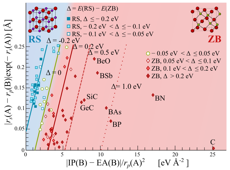
Figure 1: Predicted energy differences between RS and ZB structures of the 82 octet binary AB materials, arranged according to our optimal two-dimensional descriptor. The parallel straight lines are isolevels of the predicted model, from left to right, at -0.2, 0, 0.2, 0.5, 1.0 eV. The distance from the 0 line is proportional to the difference in energy between RS and ZB. The color/symbol code is for the reference (DFT-LDA) energies.

In closing this section, we note that the algorithm described above can be dynamically run in a web-based graphical application at:
https://analytics-toolkit.nomad-coe.eu/tutorial-LASSO_L0.

IV Cross Validation, sensitivity analysis, and extrapolation

In this section, we discuss in detail a series of analyses performed on our algorithm. We start with the adopted cross-validation (CV) scheme. Then, we investigate how the cross-validation error varies with the size of the feature space (actually, its “complexity”, as will be defined below). We proceed by discussing the stability of the choice of the descriptor with respect to sensitivity analysis. Finally, we test the extrapolation capabilities of the model.

In the numerical test described above, we have always used all the data for the training of the models; the RMSE given as figure of merit were therefore fitting errors. However, in order to assess the predictive ability of a model, it is necessary to test it on data that have not been used for the training, otherwise one can incur the so-called overfittingHastie et al. (2009). Overfitting is in general signaled by a noticeable discrepancy between the fitting error (the RMSE over the training data) and the test error (the RMSE over control data, i.e., the data that were not used during the fitting procedure). If a large amount of data is available, one can just partition the data into a training and a test set, fully isolated one from another. In our case, that is not so unusual, the amount of data is too little for such partitioning, therefore, we adopted a cross-validation strategy.

In general, the data set is still partitioned into training and test data, but this procedure repeated several times, choosing different test data, in order to achieve a good statistics. In our case, we adopted a leave-10%-out cross-validation scheme, where the data set is divided randomly into a $\sim 90$% of training data (75 data points, in our case) and a $\sim 10$% of test data. The model is trained on the training data and the RMSE is evaluated on the test set. By “training”, we mean the whole LASSO+$\ell_{0}$ procedure that selects the descriptor and determines the model (the coefficients of the linear equation) as in Eqs. (20)–(22). Another figure of merit that was monitored is the maximum absolute error over the test set. The random selection, training, and error evaluation procedure was repeated until the average RMSE and maximum absolute errors did not change significantly. In practice, we typically performed 150 iterations, but the quantities were actually converged well before. We note that, at each iteration, the standardization is applied by calculating the average and standard deviation only of the data points in the training set. In this way, no information from the test set is used in the training, while if the standardization were computed once and for all over all the available data, some information on the test set would be used in the training. In fact, it can be shown Hastie et al. (2009) that such approach can lead to spurious performance.

The cross-validation test can serve different purposes, depending on the adopted framework. For instance, in kernel ridge regression, for a Gaussian kernel, the fitted property is expressed as a weighted sum of Gaussians (see also section V): $P({\bm{d}})=\sum_{i=1}^{N}c_{i}\exp{\left(-\|{\bm{d}}_{i}-{\bm{d}}\|^{2}_{2}/2\sigma^{2}\right)}$, where $N$ is the number of training data points, i.e., there are as many coefficients as (training) data points. The coefficients $c_{i}$ are determined by minimizing $\sum_{i=1}^{N}(P({\bm{d}}_{i})-P_{i})^{2}+\lambda\sum_{i,j=1}^{N,N}c_{i}{c}_{j}\exp{\left(-\|{\bm{d}}_{i}-{\bm{d}}_{j}\|^{2}_{2}/2\sigma^{2}\right)}$, where $\|{\bm{d}}_{i}-{\bm{d}}_{j}\|^{2}_{2}=\sum_{\alpha=1}^{\Omega}(d_{i,\alpha}-d_{j,\alpha})^{2}$ is the squared $\ell_{2}$ norm of the difference of descriptors of different materials. A recommended strategy Hastie et al. (2009) is to use the cross validation to determine the optimal value of the so-called hyper-parameters, $\lambda$ and $\sigma$, in the sense that it is selected the pair $(\lambda,\sigma)$ that minimizes the average RMSE upon cross validation. In our scheme, we can regard the dimensionality $\Omega$ of the descriptor and the size $M$ of the feature space as hyper-parameters. By increasing both parameters, we do not observe a minimum, but we rather reach a plateau, where no significant improvement on the cross-validation average RMSE is achieved (see below).

Since in our procedure, the descriptor is found by the algorithm itself, a fundamental aspect of the cross-validation scheme is that all the procedure, including the selection of the descriptor, is repeated from scratch with each training set. This means that, potentially, the descriptor changes at each training-set selection. We found a remarkable stability of the 1D and 2D descriptors. The 1D was the same as the all-data descriptor (Eq. (20) for 90% of the training sets, while the 2D descriptor was the same as in Eq. (21) in all cases. For 3D and higher dimensionality, as expected from the $N=C\Omega\ln(M)$ relationship, the selection of the descriptor becomes more unstable, i.e., for different training sets, the selected descriptor often differs in at least one of the three components. The RMSE, however, does not change much from one training set to the other, i.e., the instability of the descriptor selection just reflects the presence of many competing models. We show in Table 8 the cross-validation figures of merit, average RMSE and maximum absolute error, as a function of increased dimensionality. We also show in comparison the fitting error.

Descriptor	1D	2D	3D	5D
RMSE	0.14	0.10	0.08	0.06
MaxAE	0.32	0.32	0.24	0.20
RMSE, CV	0.14	0.11	0.08	0.07
MaxAE, CV	0.27	0.18	0.16	0.12

Table 7: Root mean square error (RMSE) and maximum absolute error (MaxAE) in eV for the fit of all data (first two lines) and of the test set in a leave-10%-out cross validation (L-10%-OCV), averaged over 150 random selections of the training set (last two lines), according to our LASSO+$\ell_{0}$ algorithm.

IV.1 Complexity of the feature space

Our feature space is subdivided in 5 tiers.

• In tier zero, we have the 14 primary features as in Table 4.

• In tier one, we group features obtained by applying only one unary (e.g., $\mathcal{A}^{2},\exp(\mathcal{A})$) or binary (e.g., $|\mathcal{A}-\mathcal{B}|$) operation on primary features, where $\mathcal{A}$ and $\mathcal{B}$ stand for any primary feature. Note that in this scheme the absolute value, applied to differences, is not counted as an extra operation, i.e., we consider the operator $|\mathcal{A}-\mathcal{B}|$ as a single operator.

• In tier two, two operations are applied, e.g., $\mathcal{A}/(\mathcal{B}+\mathcal{C}),(\mathcal{A}-\mathcal{B})^{2},\mathcal{A}/\mathcal{B}^{2},\mathcal{A}\exp(-\mathcal{B})$.

• In tier three, we apply three operations: $|\mathcal{A}\pm B|/(\mathcal{C}+\mathcal{D}),|\mathcal{A}\pm\mathcal{B}|/\mathcal{C}^{2},|\mathcal{A}\pm\mathcal{B}|\exp(-\mathcal{C}),\mathcal{A}/(\mathcal{B}+\mathcal{C})^{2},\ldots$.
  

• Tier four: $|\mathcal{A}\pm\mathcal{B}|/(\mathcal{C}+\mathcal{D})^{2},|\mathcal{A}\pm\mathcal{B}|\exp(-(\mathcal{C}+\mathcal{D})),\ldots$.

• Tier five: $|\mathcal{A}\pm\mathcal{B}|\exp(-(\mathcal{C}+\mathcal{D})^{2}),\ldots$.

Our procedure was executed with tier 0, then with tier 0 AND 1, then with tiers from 0 to 2, and so on. The results are shown in Table 9. A clear result of this test is that little is gained, in terms of RMSE, when going beyond tier 3. The reason why MaxAE may increase at larger tiers is that the choice of the descriptor becomes more unstable (i.e., different descriptors may be selected) the larger the feature space is. This leads to less controlled maximal errors, and is a reflection of overfitting.

	Tier 0	Tier 1	Tier 2	Tier 3	Tier 4	Tier 5
$\Omega=1$
RMSE, CV	0.31	0.19	0.14	0.14	0.14	0.14
MaxAE, CV	0.67	0.37	0.32	0.28	0.29	0.30
$\Omega=2$
RMSE, CV	0.27	0.16	0.12	0.10	0.10	0.10
MaxAE, CV	0.60	0.39	0.27	0.18	0.19	0.22
$\Omega=3$
RMSE, CV	0.27	0.12	0.10	0.08	0.08	0.08
MaxAE, CV	0.52	0.39	0.27	0.16	0.18	0.20

Table 8: Errors after L-10%-OCV. “Tier $x$” means that all tiers up to tier $x$ are included in the feature space.

Incidentally, while for the 1D and 2D descriptor, the results presented in Eqs. (20) and (21) contain only features up to tier 3, the third component of the 3D descriptor shown in Eq. (22) belongs to tier 4. The 3D descriptor and model limited to tier 3 is:

$$\Delta E = 0.108\frac{\textrm{EA(B)}-\textrm{IP(B)}}{r_{p}(\textrm{A})^{2}}+1.790\frac{|r_{s}(\textrm{A})-r_{p}(\textrm{B})|}{\exp(r_{s}(\textrm{A}))}+$$

$$+ 3.766\frac{\left|r_{p}(\textrm{B})-r_{s}(\textrm{B})\right|}{\exp(r_{d}\textrm{({A})})}-0.0267$$

This is the same as presented in Ref. Ghiringhelli et al., 2015. The CV RMSE of the 3D model compared to the one in Eq. (22) is worse by less than 0.01 eV.

IV.2 Sensitivity Analysis

Cross validation tests if the found model is good only for the specific set of data used for the training or if it is stable enough to predict the value of the target property for unseen data. Sensitivity analysis is a complementary test on the stability of the model, where the data are perturbed, typically by random noise. The purpose of sensitivity analysis can be finding out which of the input parameters maximally affect the output of the model, but also how much the model depends on the specific values of the training data. In practice, the training data can be affected by measurement errors even if they are calculated by an ab initio model. This is because numerical approximations are used to calculate the actual values of both the primary features and the property. Since, through our LASSO+$\ell_{0}$ methodology, we determine functional relationships between the primary features and the property, applying noise to the primary features and the property is a way of finding out how much the found functional relationship is affected by numerical inaccuracies; in other words, if it is an artifact of the level of accuracy or a deeper, physically meaningful, relationship.

IV.2.1 Noise applied to the primary features

In this numerical test, each of the 14 primary features of Table 4 was independently multiplied by Gaussian noise with mean 1 and standard deviation $\sigma=0.001,0.01,0.03,0.05,0.1,0.13,0.3$, respectively. The derived features are then constructed by using these primary features including noise. We also considered multiplying by Gaussian noise (same level as for the independent features) all features at once. The test with independent features reflects the traditional sensitivity analysis test (see e.g., Ref. Meskine et al., 2009), where the goal is to single out which input parameters maximally affect the results yielded by a model. The test with all features perturbed takes into account that all primary features (as well as the fitted property) are evaluated with the same physical model and computational parameters. Therefore, inaccuracies related to not fully converged computational settings are modeled as noise.

Feature	CV scheme	Measure of Gaussian noise, $\sigma$
		0.001	0.010	0.030	0.050	0.100	0.130	0.300
IP(B)	LOOCV	99	99	98	70	4	0	0
IP(B)	L-10%-OCV	84	84	71	51	10	1	0
EA(B)	LOOCV	99	99	99	98	91	86	30
EA(B)	L-10%-OCV	86	84	84	84	80	72	28
$r_{s}(\textrm{A})$	LOOCV	99	99	99	99	96	61	0
$r_{s}(\textrm{A})$	L-10%-OCV	83	87	84	86	72	38	0
$r_{p}(\textrm{A})$	LOOCV	99	98	86	64	2	0	0
$r_{p}(\textrm{A})$	L-10%-OCV	85	85	67	42	0	0	0
$r_{p}(\textrm{B})$	LOOCV	99	99	99	99	81	50	1
$r_{p}(\textrm{B})$	L-10%-OCV	86	85	86	83	72	53	2
All 14	LOOCV	99	98	70	11	0	0	0
All 14	L-10%-OCV	85	82	52	15	0	0	0

Table 9: Number of times the 2D descriptor of the noiseless model (see Eq. 21) is found when noise is applied to the primary features. The noise is measured in terms of the standard deviation of the Gaussian-distributed set of random numbers that multiply the feature. Only for the 5 features contained in the 2D noiseless model, the noise affects the selection of the descriptor, therefore only 5 out of 14 primary features are listed. The last line shows the effect of noise applied to all primary features simultaneously. The results are displayed for both leave-one-out (LOOCV) and leave-10%-out CV schemes, as indicated by the “CV scheme” column.

Table 10 summarizes the results. It reports the fractional number of times, in %, in which the 2D descriptor of Eq. (21) is found by LASSO+$\ell_{0}$ as a function of the noise level. For each noise level, 50 random extractions of the Gaussian-distributed random number were performed. For the leave-one-out CV (LOOCV) scheme, 82 iterations were performed for each random number, i.e. each materials was once the test material. For the leave-10%-out (L-10%-OCV) 50 iterations were performed, with 50 random selections of 74 materials as training and 8 materials as test set. As expected, for the 9 primary features that do not appear in the 2D descriptor of Eq. (21), the noise does not affect the final result at any level, i.e., the 2D descriptor of the noiseless model is always found, together with the fitting coefficients.

When one of the 5 features appearing in the 2D descriptor is perturbed, the result is affected by the noise level. For noise applied to some features, the percent of selection of the 2D descriptor of the noiseless model drops faster with the noise level than for others. Of course, even when the 2D descriptor of the noiseless model is found, the fitting coefficients differ from iteration to iteration (each iteration is characterized by a different value of the random noise). For the LOOCV, the RMSE goes from 0.09 eV ($\sigma=0.001$) to 0.12 eV ($\sigma=0.3$), while for the L-10%-OCV the RMSE goes from 0.11 to 0.15 eV. So, even when, at the largest noise level, the selected descriptor may vary each time, the RMSE is only mildly affected. This reflects the fact that many competitive models are present in the feature space, and therefore a model yielding a similar RMSE can always be found. It is interesting to note that upon applying noise to IP(B) in all cases the new 2D descriptor is

$$\left(\frac{\textrm{EA(B)}}{r_{p}(\textrm{A})^{2}},\frac{|r_{s}(\textrm{A})-r_{p}(\textrm{B})|}{\exp(r_{s}(\textrm{A}))}\right),$$ (24)

i.e, the very similar to the descriptor in Eq. (21), but here IP(B) is simply missing. It is also surprising that for quite large levels of noise (10-13%) applied to EA(B), the descriptor containing this feature is selected. In general, up to noise levels of 5%, the descriptor of the noiseless model is recovered the majority of times or more. Therefore, we can conclude that the model selection is not very sensitive to the noise applied to isolated features. When the noise is applied to all features, however, the frequency of recovery of the 2D descriptor of Eq. (21) drops quickly. Still, for noise levels up to 1%, that could be related, e.g., to computational inaccuracies (non fully converged basis sets, or other numerical settings), the model is recovered almost always.

IV.2.2 Adding noise to $P=\Delta E$

We have added uniformly distributed noise of size $\delta=\pm 0.01,\pm 0.03,\ldots$ eV to the DFT data of $\Delta E$. Here, we have selected two feature spaces of size 2924 and 1568, constructed by two different set of functions, but always including the descriptors of Eqs. (20)-(22). The results are shown in Table 11. For $\Omega=2$, we report the fraction of trials for which the 2D descriptor of the unperturbed data was found in a L-10%-OCV test. (10 selection of random noise were performed and for each selection L-10%-OCV was run for 50 random selections of the training set, so the statistic is over 500 independent selections.) The selection of the descriptor is remarkably stable up to uniform noise of $\pm 0.1$ eV (incidentally, at around the value of the RMSE), then it drops rapidly. We note that the errors stay constant when the noise is in the “physically meaningful” regime, i.e., the relative ordering of the materials along the $\Delta E$ scale is not much perturbed. Only when the noise starts mixing the relative order of the materials, then the prediction becomes also less and less accurate in terms of RMSE.

Number of features	Quantity	Measure of uniform noise, $\delta$ [eV]
		$\pm 0.0$	$\pm 0.01$	$\pm 0.03$	$\pm 0.10$	$\pm 0.20$
1536	% best 2D descriptor	100	99	99	93	63
	RMSE [eV]	0.10	0.11	0.11	0.12	0.17
	AveMaxAE [eV]	0.18	0.18	0.18	0.23	0.32
2924	% best 2D descriptor	96	94	93	86	68
	RMSE [eV]	0.11	0.11	0.12	0.13	0.18
	AveMaxAE [eV]	0.19	0.20	0.22	0.24	0.34

Table 10: Performance of the model for increasing uniform noise added to the calculated $\Delta E$. Besides the RMSE and the AveMaxAE, we report the number of times, the 2D descriptor of the unperturbed data is recovered.

IV.3 Extrapolation: (re)discovering diamond

Most of machine-learning models, in particular kernel-based models, are known to yield unreliable performance for extrapolation, i.e., when predictions are made for a region of the input data where there are no training data. We note that, in condensed-matter physics, the distinction between what systems are similar and suitable for interpolation and what are not is difficult if not impossible. We test the extrapolative capabilities of our LASSO+$\ell_{0}$ methodology, by setting up two exemplary numerical tests. In the first test, we remove from the training set the two most stable ZB materials, namely C-diamond and BN (the two rightmost points in Fig. 1), and then calculate for both of them $\Delta E$, as predicted by the trained model. Although the prediction errors of 1.2 and 0.34 eV for C and BN, respectively, are very large, as can be seen in Table 11 for the 2D descriptor, the model still predicts C and BN as the most stable ZB structures. Thus, in a setup where C and BN were unknown, the model would have predicted them as good candidates to be the most stable ZB materials.

Material	$\Delta E$ [eV]		$E_{\textrm{coh}}$ [eV]
	LDA	Predicted	LDA
C	-2.64	-1.44	-10.14
BN	-1.71	-1.37	-9.72

Table 11: Performance of the model found by LASSO+$\ell_{0}$ when diamond and BN are excluded from the training. The rightmost column reports the LDA cohesive energy per atom of the ZB structure, referred to spinless atoms as used for determining the primary features in this work.

In the other test, we remove form the training set all four carbon-containing materials, namely C-diamond, SiC, GeC, and SnC, and then calculate for all of them $\Delta E$, as predicted by the trained model. The results are reported in Table 12 for the model based on the 2D descriptor. The prediction error for C-diamond is comparable to the first numerical test, and also the other errors are relatively large. However, the remarkable thing, here, is that the trained model does not know anything about carbon as a chemical element, nevertheless, it is able to predict that it will form ZB materials, and the relative magnitude of $\Delta E$ is respected.

Material	$\Delta E$ [eV]		$E_{\textrm{coh}}$ [eV]
	LDA	Predicted	LDA
C	-2.64	-1.37	-10.14
SiC	-0.67	-0.48	-8.32
GeC	-0.81	-0.46	-7.28
SnC	-0.45	-0.23	-6.52

Table 12: Performance of the model found by LASSO+$\ell_{0}$ when the carbon atom is excluded from the training, i.e., C-diamond, SiC, GeC, SnC are excluded from the training.The rightmost column reports the LDA cohesion energy per atom of the ZB structure, referred to spinless atoms as used for determining the primary features in this work.

We conclude that a LASSO+$\ell_{0}$ based model is likely to have good, at least qualitative, extrapolation capabilities. This is owing to the stability of the linear model and the physical meaningfulness of the descriptor, which contains elements of the chemistry of the chemical species building the material.

In closing this section, that we cannot draw general conclusions from the particularly robust performance of the descriptors that are found by our LASSO+$\ell_{0}$ algorithm when applied to the features space constructed as explained above. The tests described in this section, however, form a useful basis for assessing the robustness of a found model. We regard such or similar strategy to be good practice. Two criteria give us confidence that the found models may have a physical meaning: These are the particular nature of the models found by our methodology, i.e., they are expressed as explicit analytic functions of the primary features, and the evidence of robustness with respect to perturbations on the training set and the primary features. We also note that the functional relationships between a subset of the primary features and the property of interest that are found by our methodology cannot be automatically regarded as physical laws. In fact, both the primary features and $\Delta E$ are determined by the Kohn-Sham equations where the physically relevant input only consists of the atomic charges.

V Comparison to Gaussian-kernel ridge regression with various descriptors

In this section, we use Gaussian-kernel ridge regression to predict the DFT-LDA $\Delta E$ for the 82 octet binaries, with various descriptors built from our primary features (see Table 4) or functions of them. The purpose of this analysis is to point out pros and cons of using kernel ridge regression (KRR), when compared to an approach such as our LASSO+$\ell_{0}$. In the growing field of data analytics applied to materials-science problems, KRR is perhaps the machine-learning method that is most widely used to predict properties of a given set of molecules or materials Rupp et al. (2012); Pilania et al. (2013); Schütt et al. (2014); Faber et al. (2016).

KRR solves the nonlinear regression problem:

$$\mathop{\rm argmin}\limits_{\bm{c}}\sum_{j=1}^{N}\left(P_{j}-\sum_{i=1}^{N}c_{i}k({\bm{d}}_{i},{\bm{d}}_{j})\right)^{2}+\lambda\sum_{i,j=1}^{N}c_{i}k({\bm{d}}_{i},{\bm{d}}_{j}){c}_{j}$$ (25)

where $P_{j}$ are the data points, $k({\bm{d}}_{i},{\bm{d}}_{j})$ is the kernel matrix built with the descriptor ${\bm{d}}$, and $\lambda$ is the regularization parameter, with a similar role as $\lambda$ in Eqs. (3), (5), and (6). In KRR, $\lambda$ is determined by minimizing the cross-validation error. The fitting function determined by KRR is therefore $P({\bm{d}})=\sum_{i=1}^{N}c_{i}k({\bm{d}}_{i},{\bm{d}})$, i.e. a weighted sum over all the data points. The crucial steps for applying this method are the selection of the descriptor and of the kernel. The most commonly used kernel is the Gaussian kernel: $k({\bm{d}}_{i},{\bm{d}}_{j})=\exp{\left(-\|{\bm{d}}_{i}-{\bm{d}}_{j}\|^{2}_{2}/2\sigma^{2}\right)}$. The parameter determining the width of the Gaussian, $\sigma$, is recommendedHastie et al. (2009); Hansen et al. (2013) to be determined together with $\lambda$, by minimizing the cross-validation error, and this is the strategy used here. The results are summarized in Table 13. In each case, the optimal $(\lambda,\sigma)$ was determined by running LOOCV.

ID	Dim.	Descriptors	$(\lambda,\sigma)$	RMSE [eV]
1	2D	$Z_{\textrm{A}},Z_{\textrm{B}}$	$(1\cdot 10^{-6},0.008)$	0.13
2	2D	John and Bloch’s $r_{\sigma}$ and $r_{\pi}$	$(7\cdot 10^{-6},0.008)$	0.09
3	2D	our 2D	$(7\cdot 10^{-6},0.73)$	0.10
4	4D	G(A), G(B), R(A), R(B)	$(1\cdot 10^{-6},0.14)$	0.09
5	4D	$r_{s}(\textrm{A}),r_{p}(\textrm{A}),r_{s}(\textrm{B}),r_{p}(\textrm{B})$	$(2\cdot 10^{-6},0.14)$	0.08
6	5D	IP(B), EA(B), $r_{s}(\textrm{A}),r_{p}(\textrm{A}),r_{p}(\textrm{B})$	$(7\cdot 10^{-6},0.14)$	0.07
7	14D	All atomic features	$(1\cdot 10^{-6},0.42)$	0.09
8	23D	All atomic and dimer features	$(1\cdot 10^{-6},6.72)$	0.24

Table 13: Performance of the KRR method with various descriptors, in terms of the minimum cross-validation RMSE over a grid of $30\times 30$ $(\lambda,\sigma)$ values. Descriptor 4 is built with the IUPAC group (G, from 1 to 18) and period (R from row, to avoid confusion with the property ($P$)) of the elements in the PTE; performance of this set of four possible primary features with LASSO$+\ell_{0}$ is discussed in Appendix B.1. Descriptors 5 contains the 4 primary features used for building descriptor 2. Similarly, descriptor 6 contains the 5 primary features found in descriptor 3. Descriptor 7 contains all 14 atomic features listed in Table 4. Descriptor 8 contains the 14 atomic features plus 9 dimer features (see Table 16 in Appendix A).

We make the following observations:

• With several atomic-based descriptors, KRR fits reach levels of RMSE comparable to or slightly better than our fit with the LASSO+$\ell_{0}$.

• However, the performance of KRR is not improving with the dimensionality of the descriptor: Descriptor 7 contains the same features as descriptor 5 or 6, plus other, possibly relevant, features. One thus expects a better performance, which is not the case. The same happens when going to all 23 atomic and dimer features (descriptor 8).

V.1 Prediction test with KRR

We have repeated the tests as in section IV.C, i.e., we have trained a KRR model for all materials except C and BN and for all materials except all four carbon compounds. Then we have evaluated the predicted $\Delta E$ for the excluded materials. This test was done by using descriptors 1, 2, 4, 5, and 7 from Table 13. Furthermore, the 2D LASSO+$\ell_{0}$ descriptors were evaluated for the two datasets described above (details on these descriptors are given in Appendix C). These two 2D descriptors are analytical functions of five primary features each and these were also used as a 5D descriptor. In all cases, we have determined the dimensionless hyperparameters $\lambda$ and $\sigma$ by minimizing the RMSE over a LOOCV run, and the descriptors are normalized component by component. Each component of the descriptor is normalized by the $\ell_{2}$ norm of the vector of the values of that component over the whole training set. The results are shown in Tables 14 and 15.

Method	Descriptor	Dim.	($\lambda,\sigma$)	$\Delta E$(BN)	$\Delta E$(C)
LDA				-1.71	-2.64
LASSO+$\ell_{0}$	CBN	2		-1.37	-1.44
KRR	CBN	2	$(1\cdot 10^{-6},0.14)$	-2.85	-4.30
KRR	CBN∗	5	$(7\cdot 10^{-6},0.24)$	-0.96	-1.35
KRR	$Z_{\textrm{A}},Z_{\textrm{B}}$	2	$(1\cdot 10^{-6},0.0085)$	-0.68	-0.56
KRR	G(A), G(B), R(A), R(B)	4	$(1\cdot 10^{-6},0.079)$	-0.50	-1.29
KRR	$r_{\sigma}$ and $r_{\pi}$	2	$(0.013,0.045)$	-1.00	-1.17
KRR	$r_{s}(\textrm{A}),r_{p}(\textrm{A}),r_{s}(\textrm{B}),r_{p}(\textrm{B})$	4	$(1\cdot 10^{-6},0.14)$	-1.27	-2.31
KRR	All atomic features	14	$(1\cdot 10^{-6},0.42)$	-1.01	-1.91

Table 14: KRR prediction of $\Delta E$ (all in eV) for C and BN, when these two materials are not included in the training set for various descriptors, compared to the LASSO$+\ell_{0}$ result and the LDA reference. Descriptor CBN is the same 2D descriptor found by LASSO$+\ell_{0}$ for this dataset (see Table 19, row b) and descriptor CBN^∗ is built with the 5 primary features found in descriptor CBN.

Method	Descriptor	Dim.	($\lambda,\sigma$)	$\Delta E$(C)	$\Delta E$(SiC)	$\Delta E$(GeC)	$\Delta E$(SnC)
LDA				-2.64	-0.67	-0.81	-0.45
LASSO+$\ell_{0}$	$x$C	2		-1.37	-0.48	-0.46	-0.23
KRR	$x$C	2	$(1.3\cdot 10^{-5},0.079)$	-3.05	-0.66	-0.71	-0.24
KRR	$x$C∗	5	$(5.7\cdot 10^{-4},0.42)$	-2.28	-0.48	-0.44	-0.17
KRR	$Z_{\textrm{A}},Z_{\textrm{B}}$	2	$(7.3\cdot 10^{-3},0.015)$	-2.38	-0.22	-0.59	-0.29
KRR	G(A),G(B),R(A),R(B)	4	$(1\cdot 10^{-6},0.13)$	-2.28	-0.48	-0.47	-0.28
KRR	$r_{\sigma}$ and $r_{\pi}$	2	$(1.6\cdot 10^{-4},0.079)$	-1.96	-0.67	-0.50	-0.31
KRR	$r_{s}(\textrm{A}),r_{p}(\textrm{A}),r_{s}(\textrm{B}),r_{p}(\textrm{B})$	4	$(1.3\cdot 10^{-5},0.079)$	-3.06	-0.66	-0.70	-0.24
KRR	All atomic features	14	$(1\cdot 10^{-6},0.42)$	-1.55	-1.24	-0.31	-0.04

Table 15: KRR prediction of $\Delta E$ (all in eV) for all four carbon compounds, when these materials are not included in the training set for various descriptors, compared to the LASSO$+\ell_{0}$ result and the LDA reference. Descriptor $x$C^∗ is the same 2D descriptor found by LASSO$+\ell_{0}$ for this dataset (see Table 19, row d) and descriptor $x$C^∗ is built with the 5 primary features found in descriptor $x$C.

The performance of KRR in predicting the $\Delta E$ of selected subsets of materials is strongly dependent on the descriptor. In particular, when KRR is used for extrapolation (descriptor CBN, where C and BN data points are distant from the other data points in the metric defined by this 2D descriptor), the performance is rather poor in terms of quantitative error, even though still correctly predicting BN and C as very stable ZB materials. Some descriptors expected to carry relevant physical information, such as the set ($r_{s}(\textrm{A}),r_{p}(\textrm{A}),r_{s}(\textrm{B}),r_{p}(\textrm{B})$), show also good predictive ability in these examples.

In summary, KRR is a viable alternative to the analytical models found by LASSO$+\ell_{0}$ (as also noted in Ref. Kim et al., 2016), but only when a good descriptor is identified. The strength of our LASSO$+\ell_{0}$ approach is that the descriptor is determined by the method itself. Most importantly, LASSO$+\ell_{0}$ is not fooled by features that are redundant or useless (i.e., carrying little or no information on the property). These features are simply discarded. In contrast, KRR cannot discard components of a descriptor, resulting in decreasing predictive quality when a mixture of relevant and non-relevant features is naively used as descriptor.

VI Conclusions

We have presented a compressed-sensing methodology for identifying physically meaningful descriptors, i.e., physical parameters that describe the material and its properties of interest, and for quantitatively predicting properties relevant for materials-science. The methodology starts from introducing possibly relevant primary features that are suggested by physical intuition and pre-knowledge on the specific physical problem. Then, a large feature space is generated by listing nonlinear functions of the primary features. Finally, few features are selected with a compressed-sensing based method, that we call LASSO+$\ell_{0}$ because it uses the Least Absolute Shrinkage and Selection Operator for a prescreening of the features, and an $\ell_{0}$-norm minimization for the identification of the few most relevant features. This approach can deal well with linear correlations among different features. We analyzed the significance of the descriptors found by the LASSO+$\ell_{0}$ methodology, by discussing the interpolation ability of the model based on the found descriptors, the robustness of the models in terms of stability analysis, and their extrapolation capability, i.e., the possibility of predicting new materials.

VII Acknowledgment

This project has received funding from the European Union’s Horizon 2020 research and innovation program under grant agreement No 676580, The NOMAD Laboratory, a European Center of Excellence, the BBDC (contract 01IS14013E), and the Einstein Foundation Berlin (project ETERNAL). J.V. was supported by the ERC CZ grant LL1203 of the Czech Ministry of Education and by the Neuron Fund for Support of Science. This research was initiated while CD, LMG, MS, and JV were visiting the Institute for Pure and Applied Mathematics (IPAM), which is supported by the National Science Foundation (NSF).

Appendix A More details on the construction of the feature space

In order to determine the final feature space as described in section III, we proceeded in this way:

• As scalar features describing the valence orbitals, we use the radii at which the radial probability densities of the valence $s$, $p$, and $d$ orbitals have their maxima. This type of radii was, in fact, selected by our procedure, as opposed to the average radii (i.e., the quantum-mechanical expectation value of the radius). To the purpose, first two feature spaces starting from both sets of radii as primary features were constructed. In practice, in one case we started from the same primary features as in Table 4, but without group A2 (in order to reduce the dimensionality of the final space), in the other case we substituted the average radii in group $A3$, again without group $A2$. We then constructed both spaces following the rules of Tables 5 and 6. Finally, we joined the spaces and applied LASSO+$\ell_{0}$ to this joint space. Only features containing the radii at maximum were selected among the best.

• Similarly, we also defined three other radii-derived features for the atoms: the radius of the highest occupied orbital of the neutral atom, $r_{0}$, and analogously defined radii for the anions, $r_{-}$, and the cations, $r_{+}$. $r_{0}$ is either $r_{s}$ or $r_{p}$ as defined above, depending on which valence orbital is the HOMO. As in the previous point, we constructed a feature space containing both $\{r_{0},r_{-},r_{+}\}$ and $\{r_{s},r_{p},r_{d}\}$ and their combinations, and found that only the latter radii were selected among the best.

• We have considered in addition features related to the AA, BB and AB dimers (see Table 16). These new features where combined in the same way as the groups $A1$, $A2$, and $A3$, respectively (see Tables 4–6). After running our procedure, we found that features containing dimer-related quantities are never selected among the most prominent ones.

  ID	Descriptor	Symbols	#
  $A1^{\prime}$	Binding energy	$E_{b}(\textrm{AA})$, $E_{b}(\textrm{BB})$, $E_{b}(\textrm{AB})$	3
  $A2^{\prime}$	HOMO-LUMO KS gap	HL(AA), HL(BB), HL(AB)	3
  $A3^{\prime}$	Equilibrium distance	$d$(AA), $d$(BB), $d$(AB)	3

  Table 16: Set of primary features related to homo- and hetero-nuclear (spinless) dimers.

• We constructed in sequence several alternative sets of features, in particular varying systematically the elements of group $G$ (see Table 6). Multiplication of the $\{Ai,Bi,Ei\}$, $(i=1,2,3)$, by the $\{A3,B3\}$ was included, as well as division of $\{Ai,Bi,Ei\},(i=1,2,3)$, by the $\{A3,B3\}$ cubed (instead of squared ans in Table 6). Only division by $C3$ were selected by LASSO. At this stage, a descriptor in the form

  $$\left(\frac{|\textrm{IP(B)}-\textrm{EA(B)}|}{r_{p}(\textrm{A})^{2}},\,\frac{|r_{s}(\textrm{A})-r_{p}(\textrm{B})|}{r_{s}(\textrm{A})^{2}},\,\frac{\left|r_{p}(\textrm{B})-r_{s}(\textrm{B})\right|}{r_{d}\textrm{({A})}^{2}}\right)$$ (26)

  was found.

  The persistence of the $C3$ group in the denominator suggested to try other decaying functions of $r$ and $r+r^{\prime}$; for instance, exponentials as defined in $D3$ and $E3$. Interestingly, when the set of features containing $C3$, $D3$, and $E3$ was searched, the second and third component of the above descriptor were substituted by corresponding forms where the denominator squared is replaced by exponentials of the same atomic features (see below). This descriptor was therefore found by LASSO, in the sense that the substitutions $1/r_{s}(\textrm{A})^{2}\rightarrow\exp(-r_{s}(\textrm{A}))$ and $1/r_{d}\textrm{({A})}^{2}\rightarrow\exp(-r_{d}\textrm{({A})})$ are an outcome of the LASSO procedure, not of a directly attempted substitution.

• The fact that all selected features belong to group $G$ (see Table 6), which is the most populated, is not due to the fact that members of the other groups are “submerged” by the large population of group $G$ and “not seen” by LASSO. We have run extensive tests on the groups excluding $G$ and, indeed, the best-performing descriptors yield RMSE larger than those we have found.

• By noticing that the features in group $A2$ (see Table 4) never appear in the selected descriptors, and that the information carried by the features in $A1$ is similar to those in $A2$, we investigated what happens if $A1$ is removed from the primary features (and therefore all derived features containing primary features from $A1$ are removed from the feature space). We find the following models

  $$\Delta E = 0.518\frac{|\textrm{H(A)}-\textrm{L(B)}|}{\exp[r_{p}(\textrm{A})^{2}]}-0.174,$$ (27)

  $$\Delta E = 4.335\frac{r_{d}(\textrm{A})-r_{s}(\textrm{B})}{(r_{p}(\textrm{A})+r_{d}(\textrm{A}))^{2}}+16.321\frac{r_{s}(\textrm{B})}{\exp[(r_{p}(\textrm{A})+r_{p}(\textrm{B}))^{2}]}-0.406.$$ (28)

  In practice, $|\textrm{H(A)}-\textrm{L(B)}|$ replaces $|\textrm{IP(B)}-\textrm{EA(B)}|$ in the 1D model, with a similar denominator as in Eq. (21). However, the 2D model does not contain any feature from $A2$ and it is all built with features from $A3$. The RMSE of the 1D model of Eq. (27) is 0.145 eV, slightly worse than 0.142 eV for the model of Eq. (20). The RMSE of the 2D model in Eq. (28) is 0.109 eV, compared to 0.099 eV for Eq. (21). Equation (28) is also the best LASSO+$\ell_{0}$ model if the features space is constructed by using only $A3$ as primary features. In the latter case, the 1D model would be (RMSE=0.160 eV):

  $$\Delta E = 19.384\frac{r_{p}(\textrm{B})}{\exp[(r_{s}(\textrm{A})+r_{s}(\textrm{B}))^{2}]}-0.257$$ (29)

Appendix B Other feature spaces

In this Appendix, we show the performance of our algorithm with feature spaces constructed from completely different primary features than in the main text. The purpose is to underline the importance of the choice of the initial set of features. We note that when combination rules are established, performing new numerical tests takes just the (human) time to tabulate the new set of primary features for the data set.

B.1 Primary features including valence and row of the PTE

We included the “periodic-table coordinates”, period (labeled as R for Row) and group (labeled as G, from 1 to 18 according to the IUPAC numbering) as features. The reason for this test is to see whether by introducing more information than just the atomic number Z${}_{\textrm{A}}$ and Z${}_{\textrm{B}}$ (see Ghiringhelli et al., 2015), a predictive model for $\Delta E$ is obtained. The new information is the explicit similarity between elements of the same group (they share coordinate G), that is not contained in the atomic number Z. First we started with only R(A), R(B), G(A), and G(B) as primary features and constructed a features space using the usual combination rules. We note that G(B) is redundant for many but not all the cases, given G(A). In fact, for $sp$ octet binaries, the sum of the groups is 18, but for binaries containing Cu, Ag, Cd, and Zn (16 out of 82), the sum is different and therefore the coordinates are effectively 4. Next, we construct a feature space starting from the set of 14 primary fetures described in Table 4 – but where the group $A2$ (the HOMO and LUMO Kohn-Sham levels) are substituted with R(A), R(B), G(A), and G(B) – and then following the rules summarized in Tables 5and 6.

For the case where the primary features are only R(A), R(B), G(A), and G(B), we generated a feature space of size 1143 and then ran LASSO+$\ell_{0}$. The outcome is shown in Table 17. We conclude that R(A), R(B), G(A), and G(B) alone do not contain enough information for building a predictive model, following our algorithm.

	$\Omega=1$	$\Omega=2$	$\Omega=3$
RMSE [eV]	0.20	0.19	0.17
MaxAE [eV]	0.69	0.71	0.62

Table 17: Feature space with primary features R (Row or Period) and G (Group) of the PTE. Performance over the whole set of 82 materials.

For the case where the primary features are 14, including R(A), R(B), G(A), and G(B), we constructed a feature space of size 4605, and LASSO+$\ell_{0}$ found the following 1D optimal model:

$$\Delta E=-0.376+0.0944\frac{|\textrm{R(B)}-\textrm{G(B)}|}{r_{p}(\textrm{A})^{2}}.$$ (30)

In essence, $|\textrm{R(B)}-\textrm{G(B)}|$ replaced $|\textrm{IP(B)}-\textrm{EA(B)}|$ in Eq. (20), while the denominator remained unchanged. The RMSE of this new 1D model is only sightly better than the model in Eq. (20), namely 0.13 eV (vs 0.14 eV), but the MaxAE is much worse, i.e., 0.43 vs. 0.32 eV. However, this finding is remarkable as it implies some correlation between $|\textrm{R(B)}-\textrm{G(B)}|$ and $|\textrm{IP(B)}-\textrm{EA(B)}|$, where the latter is a DFT-LDA property while the former comes simply from the number of electrons and the Aufbau principle. Indeed, there is a Pearson’s correlation of 0.87 between the two quantities, while, when both quantities are divided by $r_{p}(\textrm{A})^{2}$, the Pearson’s correlation becomes as high as 0.98. The 2D and 3D optimal descriptor, though, are the same as in Eqs. (21) and (22).

Even though it is expected that the difference IP$-$EA grows when moving in the PTE to the right, a linear correlation between the difference $|\textrm{R(B)}-\textrm{G(B)}|$ and IP$-$EA it is unexpected. Figure 2 shows in the bottom panel this correlation for the $p$ elements (the anions B in the AB materials) of the PTE, while the top panel shows an even stronger linear correlation between IP$-$EA and the group G in the PTE, for each period.

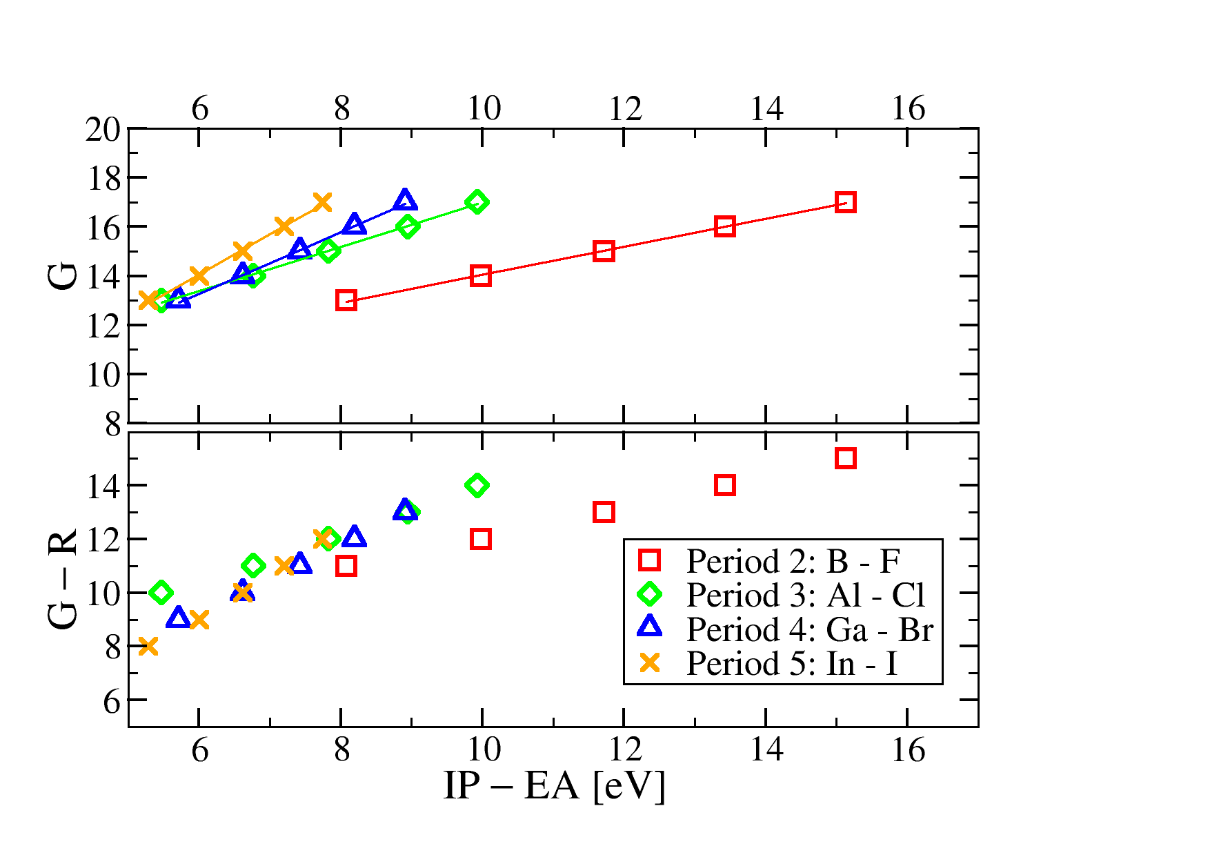
Figure 2: Plot of the difference IP$-$EA for the anions (B atoms in the AB materials) vs their Group (top pane) or the difference Group$-$Row (bottom pane) in the PTE. The straight lines are linear least-square fit of the data points

B.2 Adding John and Bloch’s $r_{\sigma}$ and $r_{\pi}$ as primary features

Here, we added $r_{\sigma}$ and $r_{\pi}$ John and Bloch (1974) to the primary features, in order to see whether combined with other features, according to our rules, yielded a more accurate and/or more robust modeling. The feature space was reduced, as plainly adding all the combinations with these 2 extra features, made the whole procedure unstable (remember that we have only 82 data points). By optimizing over a feature space of size 2924 and using all 82 materials for learning and testing, LASSO$+\ell_{0}$ identified the same 2D descriptor as in Eq. (21). In other words, no function of $r_{\sigma}$ or $r_{\pi}$ won over the known descriptor. For the L-10%-OCV, in about 10% of the cases, a descriptor containing a function of $r_{\sigma}$ or $r_{\pi}$ was selected.

B.3 Use of force constants derived from the tedrahedral pentamers AB₄ and BA₄ as primary features

Here, we build a feature space exploring the idea that the difference in energy between RS and ZB may depend on the mechanical stability of the basic constituent of either crystal structure. For instance, we choose ZB and we look at the mechanical stability of the tetrahedral pentamers AB₄ and BA₄. In practice, we look at the elastic constants for the symmetric and antisymmetric stretching deformations.

We write the elastic energy of deformation of a tetrahedral pentamer XY₄, for a symmetric stretch:

$$\Delta E_{\textrm{harm}}^{\textrm{SYMM}}=4\alpha_{\textrm{XY}}(\Delta r)^{2}$$ (31)

where $\alpha_{\textrm{XY}}$ is the bond-stretching constant (of one XY bond in the tetrahedral arrangement, which is not necessarily the same value as the one of the XY dimer). The factor 4 comes from the fact that there are 4 bonds equally stretched. The second derivative of $\Delta E_{\textrm{harm}}^{\textrm{SYMM}}$ with respect to $\Delta r$ is $(\Delta E_{\textrm{harm}}^{\textrm{SYMM}})^{\prime\prime}=8\alpha_{\textrm{XY}}$. The left-hand side is evaluated from the (LDA) calculated $\Delta E_{\textrm{harm}}^{\textrm{SYMM}}(\Delta r)$ curve, fitted to a second order polynomial.

Considering an asymmetric stretch, which means that we moved the central atom X along one of the four XY bonds, we write:

$$\Delta E_{\textrm{harm}}^{\textrm{ASYMM}} = 2\alpha_{\textrm{XY}}(\Delta r)^{2}+3\beta_{\textrm{YXY}}(\theta_{1})^{2}+3\beta_{\textrm{YXY}}(\theta_{2})^{2},$$ (32)

where $\theta_{1}$ and $\theta_{2}$ are the two different distortion angles, that the 6 angles formed by the atoms X-Y-X, undergo upon the asymmetric stretch. After working out the geometrical relationship $\theta_{1,2}^{2}=\theta_{1,2}^{2}((\Delta r)^{2})$, we find:

$$\Delta E_{\textrm{harm}}^{\textrm{ASYMM}} = 2(\alpha_{\textrm{XY}}+4\beta_{\textrm{YXY}})(\Delta r)^{2}.$$ (33)

Since the asymmetric deformation is defined through $\Delta r$, for convenience, $\beta_{\textrm{YXY}}$ is referred to the linear displacement, rather than the angular one. In practice, the relationship $\theta^{2}((\Delta r)^{2})$ was derived. The second derivative of the above expression is equated to the second derivative of the calculated $\Delta E(\Delta r)$ curve. Since $\alpha_{\textrm{XY}}$ is known from Eq. (31), $\beta_{\textrm{YXY}}$ is then inferred.

We have 4 primary features for each material, now. The first two, $\alpha_{\textrm{AB}}$ and $\alpha_{\textrm{ABA}}$, come from the AB₄ tetrahedral molecule, while the third and fourth ones, $\alpha_{\textrm{BA}}$ and $\alpha_{\textrm{BAB}}$ come from the BA₄ molecule. In addition, by noting that $\alpha_{\textrm{XY}}$ and $\beta_{\textrm{YXY}}$ enter the expression $\Delta E_{\textrm{harm}}^{\textrm{ASYMM}}$, with a ratio of 1/4, two primary features were added, i.e., $\alpha_{\textrm{AB}}+4\beta_{\textrm{ABA}}$ and $\alpha_{\textrm{BA}}+4\beta_{\textrm{BAB}}$. These 6 primary features were combined in (some of) the usual ways. Note that the above combination of $\alpha_{\textrm{BA}}$ and $\alpha_{\textrm{BAB}}$ opens a new level of complexity. At present, when constructing the feature space, we apply operations like $\textrm{A}+\textrm{B}$ and $|\textrm{A}-\textrm{B}|$, but we do not allow for the freedom of arbitrary linear combinations of them. Note also that the information about the two atoms here are intermingled in all six primary features.

To give an idea, the so obtained 2D descriptor is:

$$\left(\left[\beta_{\textrm{ABA}}-(\alpha_{\textrm{BA}}+4\beta_{\textrm{BAB}})\right]\alpha_{\textrm{AB}},\frac{\alpha_{\textrm{AB}}+4\beta_{\textrm{ABA}}+\alpha_{\textrm{BA}}+4\beta_{\textrm{ BAB}}}{\alpha_{\textrm{AB}}+\alpha_{\textrm{BA}}}\right)$$ (34)

The performance in terms of RMSE and CV is summarized in Table 18.

$\Omega$	RMSE all	RMSE CV	MAE CV	MaxAE CV
$1$	0.1910	0.1809	0.1473	0.3583
$2$	0.1532	0.1797	0.1303	0.3836
$3$	0.1346	0.2195	0.1553	0.4810

Table 18: Performance of the model built from primary features based on force-constants.

We conclude that the features based on the elastic energy do not yield a model with good predictive ability.

Appendix C Numerical tests excluding selected elements

In this numerical test, we have removed several sets of materials from the data set. In practice, we have removed:

0) Nothing
a) C-diamond (1 material)
b) C-diamond and BN (2 materials)
c) BN (1 material)
d) All carbon compounds (4 materials)
e) All boron compounds (4 materials)
f) CdO (example of a material with $\Delta E\sim 0$ (1 material))
g) All oxygen-containing compounds (7 materials)
h) All cadmium-containing compounds (4 materials)
After the removal, the usual L-10%-OCV was performed on the remaining materials. The purpose was to analyze the stability of the model when some crucial (or less crucial) elements/materials are removed completely from the data set. Also, we aimed of identifying outliers, i.e. data points whose removal from the set improve the accuracy of the fit. The results for a tier-3 feature space of size 2420 are summarized in Table 19.

Set	Dimension	RMSE [eV]	RMSE [eV]	MaxAE [eV]	Ratio	Descriptor
		all	CV	CV
0) all	1	0.14	0.15	0.28	0.85	$\mathfrak{A}$
	2	0.10	0.11	0.18	0.99	$\mathfrak{A,B}$
	3	0.08	0.09	0.17	0.95	$\mathfrak{A,B,C}$
a) no CC	1	0.12	0.14	0.29	0.91	$\mathfrak{D}$
	2	0.10	0.13	0.26	0.39	$\mathfrak{B,E}$
	3	0.08	0.08	0.17	0.91	$\mathfrak{D,B,C}$
b) no CC, BN	1	0.12	0.14	0.27	0.94	$\mathfrak{D}$
	2	0.10	0.12	0.26	0.36	$\mathfrak{D,C}$
	3	0.08	0.08	0.16	0.91	$\mathfrak{D,C,B}$
c) no BN	1	0.14	0.19	0.39	0.75	$\mathfrak{A}$
	2	0.10	0.13	0.26	0.83	$\mathfrak{A,B}$
	3	0.08	0.11	0.24	0.87	$\mathfrak{A,B,C}$
d) no C	1	0.12	0.13	0.27	0.76	$\mathfrak{F}$
	2	0.09	0.12	0.23	0.74	$\mathfrak{B,E}$
	3	0.07	0.10	0.20	0.47	$\mathfrak{D,B,C}$
e) no B	1	0.13	0.18	0.37	0.37	$\mathfrak{G}$
	2	0.10	0.14	0.30	0.42	$\mathfrak{A,B}$
	3	0.08	0.12	0.24	0.38	$\mathfrak{A,B,C}$
f) no CdO	1	0.14	0.18	0.38	0.77	$\mathfrak{A}$
	2	0.10	0.12	0.23	0.86	$\mathfrak{A,B}$
	3	0.08	0.10	0.22	0.90	$\mathfrak{A,B,C}$
g) no O	1	0.13	0.16	0.33	0.79	$\mathfrak{A}$
	2	0.10	0.13	0.27	0.74	$\mathfrak{A,B}$
	2	0.08	0.12	0.25	0.33	$\mathfrak{A,B,H}$
h) no Cd	1	0.14	0.18	0.38	0.80	$\mathfrak{A}$
	2	0.10	0.13	0.26	0.84	$\mathfrak{A,B}$
	3	0.08	0.11	0.24	0.89	$\mathfrak{A,B,C}$

Table 19: Summary of the training and CV errors for 1-, 2-, 3-dimensional descriptors for different datasets. The last column reports the descriptor found using all data in the dataset for the training and the column “Ratio” reports the fraction of times the same descriptor was found over the L-10%-OCV iterations. CC means C-diamond.

The code for the descriptors is:

$$\mathfrak{A} :\frac{\textrm{IP(B)}-\textrm{EA(B})}{r_{p}(\textrm{A})^{2}} \,\mathfrak{B} :\frac{|r_{s}(\textrm{A})-r_{p}(\textrm{B})|}{\exp(r_{s}(\textrm{A}))} \,\mathfrak{C} :\frac{|r_{s}(\textrm{B})-r_{p}(\textrm{B})|}{\exp(r_{d}(\textrm{A}))}$$

$$\mathfrak{D} :\frac{\textrm{IP(B)}}{\exp[(r_{p}(\textrm{A}))^{2}]} \,\mathfrak{E} :\frac{|\textrm{H(B)}-\textrm{L(B)}|}{r_{p}(\textrm{A})^{2}} \,\mathfrak{F} :\frac{\textrm{H(B)}}{r_{p}(\textrm{A})^{2}}$$

$$\mathfrak{G} :\frac{\textrm{IP(A)}}{[r_{s}(\textrm{A})+r_{p}(\textrm{A})]^{2}} \,\mathfrak{H} :\frac{\textrm{EA(A)}}{\exp[(r_{d}(\textrm{A}))^{2}]}$$ (35)

We make the following observations:

• When C-diamond (and C-diamond together with BN) are excluded from the set, the errors are marginally smaller. However, the descriptor changes in both cases. In particular, the 3D descriptor is remarkably stable both for b) and a).

• Removal or all 4 carbon compound leads to a similar behavior as in a) and b). However, upon removal of BN or all boron compounds leads to a fit similar to 0).

• Carbon can be thus considered as an anomaly, but it also carries important information for the stability of the overall fit.

Appendix D PYTHON script for running the LASSO algorithm with the scikit_learn library

⬇

from sklearn import linear_model

lasso = sklearn.linear_model.Lasso(alpha=lambda)

lasso.fit(D,P)

coefficients = lasso.coef_

Here sklearn solves the problem in Eq. (6), with the $\ell_{2}$-norm scaled by a factor $\frac{1}{2N}$. The bias $c_{0}$ is included by default.

References

- (1) Springer Materials, Landolt-Börnstein, “The most comprehensive collection of data in the fields of physics, physical and inorganic chemistry, materials science, and related fields”; http://materi- als.springer.com/.
- Lorenz et al. (2004) S. Lorenz, A. Groß, and M. Scheffler, Chem. Phys. Lett. 395, 210 (2004).
- Hautier et al. (2010) G. Hautier, C. C. Fischer, A. Jain, T. Mueller, and G. Ceder, Chem. Mater. 22, 3762 (2010).
- Behler (2011) J. Behler, Phys. Chem. Chem. Phys. 13, 17930 (2011).
- Pilania et al. (2013) G. Pilania, C. Wang, X. Jiang, S. Rajasekaran, and R. Ramprasad, Scientific Reports 3, 2810 (2013).
- Szlachta et al. (2014) W. Szlachta, A. Bartók, and G. Csányi, Phys. Rev. B 90, 104108 (2014).
- Mueller et al. (2014) T. Mueller, E. Johlin, and J. Grossman, Phys. Rev. B 89, 115202 (2014).
- Schütt et al. (2014) K. Schütt, H. Glawe, F. Brockherde, A. Sanna, K. Müller, and E. Gross, Phys. Rev. B 89, 205118 (2014).
- Atsuto et al. (2015) S. Atsuto, A. Togo, H. Hayashi, K. Tsuda, L. Chaput, and I. Tanaka, Phys. Rev. Lett. 115, 205901 (2015).
- Faber et al. (2015) F. Faber, A. Lindmaa, O. von Lilienfeld, and R. Armiento, Int. J. Quantum Chemistry 115, 1094 (2015).
- Caccin et al. (2015) M. Caccin, Z. Li, J. Kermode, and A. De Vita, Int. J. Quantum Chemistry 115, 1129 (2015).
- Isayev et al. (2015) O. Isayev, D. Fourches, E. N. Muratov, C. Oses, K. Rasch, A. Tropsha, and S. Curtarolo, Chem. Mater. 27, 753 (2015).
- Mannodi-Kanakkithodi et al. (2016) A. Mannodi-Kanakkithodi, G. Pilania, T. Doan Huan, T. Lookman, and R. Ramprasad, Sci. Reports 6, 20952 (2016).
- Kim et al. (2016) C. Kim, G. Pilania, and R. Ramprasad, Chem. Mater. 28, 1304 (2016).
- Ueno et al. (2016) T. Ueno, T. Rhone, Z. Hou, T. Mizoguchi, and K. Tsuda, Materials Discovery, in press (2016).
- Solovyeva and von Lilienfeld (2016) A. Solovyeva and O. von Lilienfeld, arXiv:1605.08080 (2016).
- Bialon et al. (2016) A. F. Bialon, T. Hammerschmidt, and R. Drautz, Chem. Mater. 28, 2550 (2016).
- Ghiringhelli et al. (2015) L. M. Ghiringhelli, J. Vybiral, S. V. Levchenko, C. Draxl, and M. Scheffler, Phys. Rev. Lett. 114, 105503 (2015).
- Donoho (2006) D. Donoho, IEEE Trans. Inform. Theory 52, 1289 (2006).
- Candès and Wakin (2008) E. J. Candès and M. B. Wakin, IEEE Signal Processing Magazine 25, 21 (2008).
- Davenport et al. (2012) M. Davenport, M. Duarte, Y. Eldar, and G. Kutyniok, Introduction to compressed sensing: Theory and Applications (Cambridge University Press, 2012).
- Boche et al. (2015) H. Boche, R. Calderbank, G. Kutyniok, and J. Vybiral, Compressed sensing and its applications (2015).
- Guyon and Elisseeff (2003) I. Guyon and A. Elisseeff, J. Mach. Learn. Res. 3, 1157 (2003).
- Kohn and Sham (1965) W. Kohn and L. Sham, Phys. Rev. 140, A1133 (1965).
- Hohenberg and Kohn (1964) P. Hohenberg and W. Kohn, Phys. Rev. 136, B864 (1964).
- Ceperley and Alder (1980) D. M. Ceperley and B. J. Alder, Phys. Rev. Lett. 45, 566 (1980).
- Perdew and Wang (1992) J. P. Perdew and Y. Wang, Phys. Rev. B 45, 13244 (1992).
- van Vechten (1969) J. A. van Vechten, Phys. Rev. 182, 891 (1969).
- Phillips (1970) J. C. Phillips, Rev. Mod. Phys. 42, 317 (1970).
- Bloch and Simons (1972) A. N. Bloch and G. Simons, J. Am. Chem. Soc. 94, 8611 (1972).
- John and Bloch (1974) J. S. John and A. Bloch, Phys. Rev. Lett. 33, 1095 (1974).
- Zunger (1980) A. Zunger, Phys. Rev. B 22, 5839 (1980).
- Chelikowsky (1982) J. Chelikowsky, Phys. Rev. B 26, 3433 (1982).
- Pettifor (1984) D. G. Pettifor, Solid State Commun. 51, 31 (1984).
- Villars (1985) P. Villars, Less-Common Met. 109, 93 (1985).
- Andreoni et al. (1985) W. Andreoni, G. Galli, and M. Tosi, Phys. Rev. Lett. 55, 1734 (1985).
- Andreoni and Galli (1987) W. Andreoni and G. Galli, Phys. Rev. Lett. 58, 2742 (1987).
- Saad et al. (2012) Y. Saad, D. Gao, T. Ngo, S. Bobbitt, J. R. Chelikowsky, and W. Andreoni, Phys. Rev. B 85, 104104 (2012).
- Bertsekas (1999) D. P. Bertsekas, Nonlinear Programming (Athena Scientific, 1999).
- Arora and Barak (2009) S. Arora and B. Barak, Computational Complexity: A Modern Approach (University Press, Cambridge, 2009).
- Tibshirani (1996) R. Tibshirani, J. Royal Statist. Soc. B 58, 267 (1996).
- Hastie et al. (2009) T. Hastie, R. Tibshirani, and J. Friedman, The elements of statistical learning (Springer, New York, 2009).
- Greenshtein (2006) E. Greenshtein, Ann. Statist. 34, 2367 (2006).
- van de Geer (2008) S. van de Geer, Ann. Statist. 36, 614 (2008).
- Bühlmann and van de Geer (2011) P. Bühlmann and S. van de Geer, Statistics for High-Dimensional Data (Springer, Berlin, 2011).
- Cohen et al. (2009) A. Cohen, W. Dahmen, and R. DeVore, J. Am. Math. Soc. 22, 211 (2009).
- Gross et al. (2010) D. Gross, Y.-K. Liu, S. T. Flammia, S. Becker, and J. Eisert, Phys. Rev. Lett. 105, 150401 (2010).
- Blum et al. (2009) V. Blum, R. Gehrke, F. Hanke, P. Havu, V. Havu, X. Ren, K. Reuter, and M. Scheffler, Comp. Phys. Comm. 180, 2175 (2009).
- van Lenthe et al. (1994) E. van Lenthe, E. J. Baerends, and J. G. Snijders, J. Chem. Phys. 101, 9783 (1994).
- (50) We used for IP (EA) the energy of the half occupied Kohn-Sham orbital in the half positively (negatively) charged atom.
- Simons and Bloch (1973) G. Simons and A. N. Bloch, Phys. Rev. B 7, 2754 (1973).
- Chelikowsky and Phillips (1978) J. R. Chelikowsky and J. C. Phillips, Phys. Rev. B 17, 2453 (1978).
- Andreoni et al. (1979) W. Andreoni, A. Baldereschi, E. Biémont, and J. C. Phillips, Phys. Rev. B 20, 4814 (1979).
- Cor (a) Differently from H L and IP EA, which are expected, and are, correlated on physical grounds for all atoms, is not necessairly expected to be correlated to . This is true for all the atoms considered in this work, but it could well be that such strong correlation is not valid for all atoms. This situation is somewhat reminiscent of the Berkson paradox, i.e., when a spurious correlation is found due to a biased selection of the data set.
- Hofmann et al. (2008) T. Hofmann, B. Schölkopf, and A. J. Smola, Ann. Stat. 36, 1171 (2008).
- (56) “Having a large correlation” is clearly not a transitive relationship, i.e., if the vector is highly correlated with (the absolute value of the covariance is close to 1), and is highly correlated to , is not necessarily highly correlated to .
- Nelson et al. (2013a) L. J. Nelson, G. L. W. Hart, F. Zhou, and V. Ozoliņs̆, Phys. Rev. B 87, 035125 (2013a).
- Nelson et al. (2013b) L. Nelson, V. Ozoliņš, C. Reese, F. Zhou, and G. L. W. Hart, Phys. Rev. B 88, 155105 (2013b).
- Ozoliņš et al. (2013) V. Ozoliņš, R. Lai, R. Caflisch, and S. Osher, Proc. Natl. Acad. Sci. USA 110, 18368 (2013).
- Zhou et al. (2014) F. Zhou, W. Nielson, Y. Xia, and V. Ozoliņš, Phys. Rev. Lett. 113, 185501 (2014).
- Budich et al. (2014) J. Budich, J. Eisert, E. Bergholtz, S. Diehl, and P. Zoller, Phys. Rev. B 11, 115110 (2014).
- J.R. (1998) K. J.R., Genetic Programming (MIT PRess, 1998).
- Candés et al. (2006) E. J. Candés, J. Romberg, and T. Tao, IEEE Trans. Inform. Theory 52, 489 (2006).
- Foucart and Rauhut (2013) S. Foucart and H. Rauhut, A mathematical introduction to compressive sensing (Springer, New York, 2013).
- (65) With signs this is St. John & Bloch’s , with signs it is .
- Cor (b) Correlation between pairs of features means in this context that the absolute value of the covariance (i.e., the scalar product of the 82-dimensional vectors containing the values of features and , with each vector subtracted of its mean value and divided by its standard deviation) is close to 1. If their covariance is close to zero, the two features are uncorrelated.
- Meskine et al. (2009) H. Meskine, S. Matera, M. Scheffler, K. Reuter, and H. Metiu, Surf. Sci. 603, 1724 (2009).
- Rupp et al. (2012) M. Rupp, A. Tkatchenko, K.-R. Müller, and O. A. von Lilienfeld, Phys. Rev. Lett. 108, 058301 (2012).
- Faber et al. (2016) F. A. Faber, A. Lindmaa, O. A. von Lilienfeld, and R. Armiento, Phys. Rev. Lett. 117, 135502 (2016).
- Hansen et al. (2013) K. Hansen, G. Montavon, F. Biegler, S. Fazli, M. Rupp, M. Scheffler, O. A. von Lilienfeld, A. Tkatchenko, and K.-R. Müller, JCTC 9, 3404 (2013).