Electron acceleration at pulsar wind termination shocks

Abstract

We study the acceleration of electrons and positrons at an electromagnetically modified, ultra-relativistic shock in the context of pulsar wind nebulae (PWNe). We simulate the outflow produced by an obliquely rotating pulsar in proximity of its termination shock with a two-fluid code which uses a magnetic shear wave to mimic the properties of the wind. We integrate electron trajectories in the test-particle limit in the resulting background electromagnetic fields to analyse the injection mechanism. We find that the shock-precursor structure energizes and reflects a sizeable fraction of particles, which becomes available for further acceleration. We investigate the subsequent first-order Fermi process sustained by small-scale magnetic fluctuations with a Monte Carlo code. We find that the acceleration proceeds in two distinct regimes: when the gyro-radius $r_{\textrm{g}}$ exceeds the wavelength of the shear $\lambda$, the process is remarkably similar to first-order Fermi acceleration at relativistic, parallel shocks. This regime corresponds to a low density wind which allows the propagation of superluminal waves. When $r_{\textrm{g}}<\lambda$, which corresponds to the scenario of driven reconnection, the spectrum is softer.

1. Introduction

In this paper we address the mechanisms by which relativistic particles are accelerated in pulsar wind nebulae (PWNe). The broad-band non-thermal radiation emitted by these objects is normally modeled as Synchrotron and inverse Compton emission from a population of high-energy electrons and positrons (here collectively referred to as “electrons”) distributed in a broken power-law spectrum. These particles are presumably accelerated at, or close to, the termination shock (TS) of the relativistic pulsar wind, which is located roughly where its momentum flux density is balanced by the confining pressure of the external medium (for young, isolated pulsars, the parent supernova remnant, for older ones, the interstellar medium). The electron spectrum $N(\gamma)\propto\gamma^{-s}$ is hard ($s\sim 1.5$) at the low energies responsible for the radio to optical emission, and softens ($s\gtrsim 2.2$) at the high energies responsible for the $X$-ray Synchrotron emission. The X-ray morphology suggests that electrons are preferentially accelerated in the equatorial belt of an almost axisymmetric structure (Kirk et al., 2009b; Amato, 2014; Porth et al., 2014; Olmi et al., 2015).

In the best observed source — the Crab Nebula — the power-law index at high energies is close to that predicted for first-order Fermi acceleration at a parallel, ultra-relativistic shock front (Bednarz & Ostrowski, 1998; Kirk et al., 2000; Achterberg et al., 2001). At first sight, this is surprising, since the magnetic field is not expected to be normal to the TS. On the contrary, the field is embedded in the radial pulsar wind and is tightly wound up by the rotating neutron star. In an axisymmetric wind, this leads to a perpendicular magnetic field configuration over almost the entire surface of the TS, and, consequently, to strong suppression of the Fermi process (Begelman & Kirk, 1990; Sironi & Spitkovsky, 2009; Summerlin & Baring, 2012; Sironi et al., 2015).

Axisymmetry, however, is a good approximation only far from the neutron star. Close to the surface of the star, the boundary conditions impose a non-axisymmetric structure, which is frequently modeled as an inclined magnetic dipole (e.g., Michel, 1991). In the region in which the wind is launched, this structure is converted into a wave with an alternating magnetic field in the equatorial zone (Tchekhovskoy et al., 2016). Magnetic reconnection in the equatorial zone was originally suggested by Coroniti (1990) as a way of energizing electrons in a “striped wind”. Although subsequent work suggests that the process is too slow to annihilate the field completely before the wind encounters the TS (Lyubarsky & Kirk, 2001; Kirk & Skjæraasen, 2003), it nevertheless remains a promising possibility, in particular for the production of gamma-ray pulses (Mochol & Pétri, 2015; Cerutti et al., 2016) and flares (Arons, 2012; Baty et al., 2013; Takamoto et al., 2015).

Therefore, given that reconnection is unlikely to be complete, the equatorial zone of the wind arriving at the TS will contain a substantial oscillating component of the magnetic field. Although oriented perpendicular to the shock normal, this field is nevertheless available for dissipation (Lyubarsky, 2003). The dissipation process itself can pictured in two scenarios, depending on the local value of the plasma density:

1. In a high-density plasma, the equations of MHD can be expected to give a good description of the dynamics except close to surfaces at which the polarity of the field reverses. In this case, the simplest picture of the structure of the TS is one in which the magnitude of the magnetic field in the upstream plasma is constant, but its direction reverses at current sheets embedded in the flow. At the TS, a fast-mode shock compresses the magnetized parts as in the standard MHD picture. Because the plasma is strongly magnetized, the shock is weak, and does not significantly dissipate the magnetic energy (Kennel & Coroniti, 1984). However, the compression of the embedded current sheets triggers reconnection inside them, a phenomenon referred to as “driven reconnection”. As the sheets are advected downstream in the compressed, striped pattern, dissipation becomes more and more important, causing them to expand and, ultimately, completely disrupt the pattern, thereby releasing the magnetic energy (Pétri & Lyubarsky, 2007; Sironi & Spitkovsky, 2011).

2. In a low-density plasma, the equations of MHD fail because of a lack of charge-carrying particles. This happens when the characteristic scale on which the fields in the upstream plasma vary — in this case the rotation frequency of the pulsar — is faster than the intrinsic frequency of non-MHD waves, which is the local plasma frequency, possibly modified by relativistic effects. The most important non-MHD waves in this context are transverse, electromagnetic modes. In the limit of low density, these correspond to vacuum waves that propagate at $c$. At finite plasma density, their group speed is subluminal, but their phase speed exceeds $c$, giving rise to the nomenclature “superluminal waves”(Arka & Kirk, 2012; Mochol & Kirk, 2013a, b). In this parameter regime, the simplest picture of the structure of the TS is again one in which the magnitude of the magnetic field in the upstream plasma is constant, but, instead of reversing direction at a current sheet, the magnetic vector rotates smoothly in a monochromatic, static shear. At the TS, this pattern converts into superluminal waves, some of which propagate back into the upstream plasma, and dissipate there in an “electromagnetic precursor”(Amano & Kirk, 2013).

In a realistic system, the pulsar wind upstream of the TS will not correspond exactly to either the striped case, or the monochromatic, static shear, so that elements of each scenario may be present. However, their relative importance will depend primarily on the ratio of the pulsar frequency to the local plasma frequency. For almost all isolated pulsars, this is a large number at the TS (Arka & Kirk, 2012). Therefore, we concentrate in this paper on particle acceleration in the low density scenario 2.

First, we use the two-fluid code described in Amano & Kirk (2013) to generate a realization of the turbulent electromagnetic fields in the proximity of the TS, and examine the fate of test-particles moving in these fields. We find that a sizeable fraction of these decouples from the fluid flow and is reflected, thereby becoming available for further acceleration via the first-order Fermi mechanism. Assuming that small-scale magnetic fluctuations scatter particles in both the upstream and downstream plasma, we then use a Monte Carlo (MC) code to simulate this acceleration process, in which particles cross and recross the compound TS layer, consisting of an electromagnetic precursor and shock compression. Despite the fact that the upstream plasma contains an oscillating magnetic field oriented perpendicular to the shock normal, we find that in the regime where superluminal waves propagate, the spectral index of accelerated particles is close to that predicted for a parallel shock, whereas, for high-energy particles, a softer spectrum is predicted for the regime of driven reconnection.

The paper is organized as follows. In Sect. 2 we describe the two-fluid simulation, in 3 the test-particle integration, and, in 4, the Monte-Carlo simulations. The implications of our results are discussed in Sect. 5 and compared with results obtained in the high density, driven reconnection regime. Section 6 summarizes our main conclusions.

2. Two-fluid simulation

Numerical simulation of the structure of the TS in the low-density regime presents a challenge. Sophisticated, 3D-MHD simulations are capable of addressing the global structure downstream of the TS and the problem of dissipation in the pulsar wind nebula (e.g., Porth et al., 2014), but these assume that all fluctuations at the pulsar rotation frequency have been damped away. Particle-in-cell simulations, on the other hand, are not limited by this assumption, but they are computationally intensive. To date, they have been performed in 2D and 3D, but only in the high-density regime, where an extended, electromagnetic precursor does not form (Sironi & Spitkovsky, 2011; Takamoto et al., 2015). At present, the most promising method available is two-fluid simulation, in which the electrons and positrons constitute separate, charged fluids that are coupled by Maxwell’s equations (Zenitani et al., 2009; Barkov & Komissarov, 2016).

Amano & Kirk (2013) used a relativistic, two-fluid (electron and positron) code (1D in space, 3D in velocity and electromagnetic fields) to show that superluminal waves strongly modify the TS when the ambient density is low enough to permit the propagation of these waves. They discussed in detail the dissipation processes in the electromagnetic precursor upstream of the main compression, which resembles a hydrodynamics sub-shock. Whether or not this complex structure is also capable of dissipating energy into a population of accelerated, non-thermal particles extending over a broad range in energy depends crucially on its ability to reflect some of the particles that make up the incoming fluids (e.g., Sironi & Spitkovsky, 2009). To attack this question, we first use the two-fluid code to generate an example of such a precursor that has reached a long-lived, quasi-steady state.

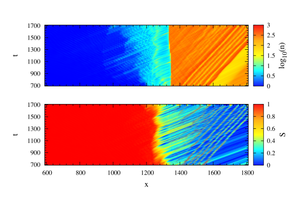
Figure 1.— Time evolution of the modified shock structure. The top and bottom panels show the proper density and the normalized Poynting flux profiles, respectively. We show only the phase with a quasi-stationary precursor.

The set-up and parameters we choose are similar to those discussed by Amano & Kirk (2013). A sinusoidal, circularly polarized, transverse magnetic shear is assumed to be incident on the upstream boundary. In the following, we use the expressions “shear wave”and “striped wind”interchangeably. We define a frame of reference called the URF (upstream rest frame) in which the electric field of this wave vanishes. Denoting quantities measured in this frame by a bar, and using cartesian coordinates with $x$ along the shock normal, its magnetic field is

$$\overline{B}_{y}=+\overline{B}_{0}\cos(\overline{k}_{0}\overline{x})$$ (1)

$$\overline{B}_{z}=-\overline{B}_{0}\sin(\overline{k}_{0}\overline{x})\,.$$ (2)

The corresponding current is everywhere parallel to the magnetic field, whose magnitude is constant, so that the wave is, in fact, a force-free equilibrium. The proper density $n_{0}$ of the positron fluid equals that of the electron fluid and is constant; the velocity $\overline{v}_{0}$ of the positron fluid, is parallel to $\overline{\bf B}$ and constant in magnitude (the electron fluid velocity is $-\overline{v}_{0}$).

By a suitable choice of downstream boundary conditions, the reference frame in which the simulation is performed (called the SRF — shock/simulation rest frame) is arranged to coincide with that in which the shock-precursor structure is almost stationary. Seen from this frame, the URF moves along the $x$-axis at the “shock speed” $c\beta_{\rm s}$, which equals the phase speed of the incoming wave. Using unadorned symbols for quantities measured in the SRF, the incoming wave has wavenumber and frequency given by $k=\Gamma_{\rm s}\overline{k}$, $\omega=c\beta_{\rm s}\Gamma_{\rm s}\overline{k}$, where the “shock Lorentz factor” $\Gamma_{\rm s}=1/\sqrt{1-\beta_{\rm s}^{2}}$. Assuming the pulsar moves slowly with respect to the TS, we identify the wave frequency with its rotation frequency.

Three dimensionless parameters are required to specify the initial conditions for the simulation. In addition to $\Gamma_{\rm s}$, these are the ratio $\Omega$ of the incoming wave frequency to the proper plasma frequency associated with $n_{0}$: $\Omega=\omega/\omega_{{\rm p}0}$, $\omega_{{\rm p}0}=\left(8\pi n_{0}e^{2}/m\right)^{1/2}$, and the incoming magnetization parameter $\sigma_{0}$ (defined below). Our choice of $\Omega$ is restricted, on the one hand, to $\Omega>1$ by the requirement that superluminal waves can propagate (see e.g., Arka & Kirk, 2012). On the other hand, in order to find a precursor that is contained within the simulation box, we find that $\Omega\lesssim 2$. Therefore, following Amano & Kirk (2013), we choose $\Omega=1.2$ as a representative value. In order to correspond to pulsar conditions, the shock Lorentz factor $\Gamma_{\rm s}$ should be $\sim 10^{4}$ or larger, but its value in the simulation is limited by technical issues associated with code stability, and we adopt a compromise value of $\Gamma_{\rm s}=100$. Finally, the magnetization parameter $\sigma$ is defined in the simulation as the ratio of the fluxes in the $x$ direction of electromagnetic energy and particle enthalpy. However, the requirement that the shock speed should greatly exceed the speed of the fast magnetosonic wave: $\Gamma_{\rm s}\gg\sigma_{0}^{1/2}$, implies that the velocity of the fluids in the URF is non-relativistic: $\overline{v}_{0}/c\approx\Omega\sigma_{0}^{1/2}/\Gamma_{\rm s}\ll 1$, in which case, $\sigma_{0}\approx\overline{B}_{0}^{2}/\left(8\pi n_{0}mc^{2}\right)$. In our simulation, we select $\sigma_{0}=25$, giving $\overline{v}_{0}=0.06\,c$, and fix a cool initial fluid temperature corresponding to a thermal velocity of $0.14\,c$.

The resulting profiles of density and Poynting flux are shown in Fig. 1 where time and space are plotted in units of $1/\omega_{{\rm p}0}$ and $c/\omega_{{\rm p}0}$, respectively. We confirm the findings of Amano & Kirk (2013) that the breakout of the precursor is triggered by the launch of superluminal waves which lead to the dissipation of the Poynting flux $S$ carried by the incoming wave into enthalpy of the plasma. As can be seen in the top and middle panels of Fig.  2, where we plot the pressure and the longitudinal component of the four-velocity of the plasma at $t=1700$, the dissipation is, at least in part, due to the formation of small-scale shocks. These decelerate and heat the plasma before it encounters the hydrodynamic sub-shock, which is located at $x_{\textrm{s}}=1335$ and is represented by the black solid line in Fig. 2. In this figure, we depict the “precursor” as that region located between the sub-shock and the point $x_{\textrm{p}}=1175$, marked with a dashed black line, where the bulk of the Poynting flux is dissipated. Here, there is a strong increase in plasma temperature and pressure, which lowers the local plasma frequency, thereby permitting the propagation of low frequency superluminal modes. Further upstream, the plasma is still perturbed by the propagation of superluminal waves, but dissipation is limited to increasing the plasma enthalpy at the expense of its kinetic energy. This structure can be identified in Fig. 1, by comparing the extension of the region upstream of the shock where the plasma density increases (the cyan region in the top panel) with the region where the Poynting flux has its maximum value (red region in the bottom panel). It can also be seen in fig. 2, by comparing the spatial profile of the Poynting flux with that of the plasma velocity at $t=1700$.

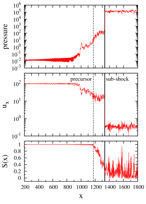
Figure 2.— Pressure (top panel), $x$ component of the plasma four-speed (middle panel) and normalized Poynting flux (bottom panel) profiles at $t=1700$. The solid and dashed black lines represent the position of the hydrodynamic sub-shock and leading edge of the precursor, respectively.

In the precursor, the Poynting flux carried by the incoming wave is almost completely converted into plasma enthalpy, as shown in the bottom panels of both Fig. 1 and 2, leaving a region of turbulent fields downstream of the shock. Here, the amplitude of the turbulence decreases as the distance to the shock increases, showing that the magnetic field of the incoming shear wave is completely annihilated.

3. Test-particle trajectories

To assess the ability of the TS to energize and potentially reflect individual particles, we extract, from the simulation described above, the electromagnetic fields in a space-time volume in which a quasi-stationary precursor is established, and follow the trajectories of test particles in these fields.

Two technical issues arise in extracting the fields. Firstly, they are stored as vector quantities on a fixed grid in space-time. In order to limit the data to a manageable volume, we keep the spatial grid used in the two-fluid code (i.e., $4\times 10^{4}$ points) and store snapshots (typically 2000) taken at intervals of $\omega_{{\rm p}0}^{-1}$. Since we use an adaptive time-step to advance the test-particle trajectories, it is necessary to interpolate the fields on this two-dimensional grid. For this purpose, we use a 2-D cubic-spline algorithm (see Press et al., 1986), which ensures continuity and differentiability of the interpolated function and its first derivative, whilst avoiding spurious oscillations between grid points.

Secondly, examination of Fig. 1 shows that the precursor can be regarded as quasi-stationary for times $t>700$. Thus, the total time for which we are able to simulate this turbulence is limited to $t\lesssim 1000$. However, test particles can potentially spend a much longer time in the precursor before being transmitted or reflected. We deal with this problem by imposing periodic boundaries in time on the fields, i.e., by folding as many times as necessary the subset of snapshots between $t=700$ and $t=700+\tau$. To check that this procedure does not introduce artifacts, we integrate several thousand trajectories, building the electron spectrum and angular distribution at both the upstream and downstream spatial boundaries for $\tau=250$, $500$, $1000$.

With this method, we obtain a representation of the spatial and temporal dependence of the turbulent electric and magnetic fields in the precursor, that covers fluctuations on timescales between $\omega_{{\rm p}0}^{-1}$ and $1000\omega_{{\rm p}0}^{-1}$, and length scales between $10^{-2}\,\lambda$ and the size of the computational box, roughly $500\lambda$. These fields are responsible for scattering and pre-accelerating super-thermal test-particles that are drawn from the electron and positron fluids.

The test-particle integration procedure itself employs a standard fourth-order Runge-Kutta algorithm, with the adaptive time-step routine described by Press et al. (1986). This is applied to the equations of motion written in the form given by Kirk et al. (2009a), but excluding the effects of radiation reaction. All trajectories are initiated far upstream of the shock using one of two prescriptions:

1. The initial four-momentum equals that of the electron fluid at that time-space point. We use this prescription to study how and where the difference between fluid and test particle trajectories manifests itself.

2. The initial four momentum seen in the URF is randomly (isotropically) distributed in angle and uniformly in Lorentz factor over the range $[1:1.2]$. With this prescription test-electrons have roughly the same energy as background electrons, but decouple more rapidly from the fluid flow.

Each trajectory is followed until it terminates upon reaching either the upstream or the downstream edge of the simulation box. The reflection probability is then the ratio of the number of trajectories that terminate at the upstream absorbing boundary to the total number of trajectories.

Typical electron trajectories are plotted in Fig. 3, where the black solid line represents the position of the sub-shock and the black dashed line represents the approximate position of the leading edge of the precursor. Trajectories 1-3 are initiated with the same four-momentum as a local fluid element (prescription 1). Trajectory 4 (for clarity plotted with a small off-set in time) starts with $\overline{\gamma}=1.001$ and a random direction in the local fluid frame (prescription 2) at the same

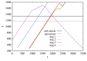
Figure 3.— Typical electron trajectories in the proximity of the sub-shock (black solid line) and of its precursor (black dashed line). Trajectories 1-3 are initiated as fluid elements (prescription 1). Trajectory 4 is initiated as a test-particle (prescription 2) at the same location and time of trajectory 2 (for clarity plotted with a small off-set in time).

time and position as trajectory 3. Test electrons obey the same equations of motion as the fluid elements, except that the latter have an additional pressure force that prevents them intersecting each other. Consequently, test particles decouple from the background plasma when the pressure term becomes appreciable. The fate of characteristic trajectories is shown in Fig. 3. Particles can travel across the shock with very little deflection (trajectory 2) or undergo several reversals (changes in the sign of $\beta_{x}$, trajectories 1, 3 and 4). If they experience one or more reversals, electrons can subsequently be registered at either one of the two spatial boundaries. We find that the first reversal can only occur downstream of the sub-shock, whereas the following can occur on either side of the sub-shock.

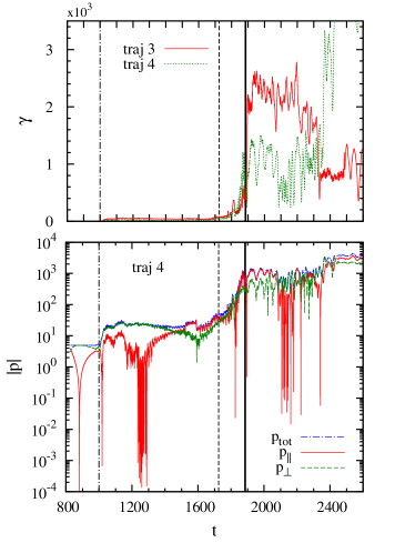
Figure 4.— Top panel: Comparison of the electron Lorentz factor expressed in the frame comoving with the fluid along $x$ for trajectories 3 and 4. Bottom panel: Total (blue), longitudinal (red) and transverse (green) electron momentum for trajectory 4 expressed in the same frame. In both panels the vertical solid, dashed and dot-dashed black lines represent the sub-shock, precursor and superluminal wave-front, respectively.

In Fig. 4 we plot the electron Lorentz factor for trajectories 3 and 4 (top panel) and the components of the electron momentum (total (blue), longitudinal (red) and transverse (green)) for trajectory 4 in a frame moving along the $x$-axis at the same speed as the charged fluids (each of which has, to high accuracy, the same $x$-velocity). The vertical dot-dashed, dashed and solid black lines represent the time at which an electron crosses the superluminal wave-front, the leading edge of the precursor and the hydrodynamic sub-shock, respectively. The top panel of Fig. 4 along with Fig. 3, shows that there is no significant difference between the trajectory and temporal behavior of the Lorentz factor between the two prescriptions used to initiate the electron trajectory. For both prescriptions, as seen in the frame comoving with the fluids, test particles move with the plasma until they cross the superluminal wave-front. There, the Lorentz factor slightly increases and subsequently stays almost constant until the electrons reach the leading edge of the precursor. In the precursor, the total energy of test particles is enhanced by almost two orders of magnitude. When electrons move downstream of the shock their Lorentz factor oscillates about a constant value unless, as in the specific cases under consideration (trajectories 3 and 4), more reversals occur, which can cause a change in the total energy. The bottom panel of Fig. 4 shows that the transverse momentum of an electron whose trajectory is initiated with prescription 2 dominates over its longitudinal momentum almost up to the leading edge of the precursor. Close to the precursor the longitudinal momentum takes over and dominates the energy balance for the rest of the trajectory. Whether the energized electrons are transmitted to the downstream absorbing boundary or reflected to the upstream one depends on their parallel momentum and on the degree of turbulence they encounter in the downstream. The reason for this is that if the parallel momentum is large, or, conversely, the magnetic field they encounter is small, their gyro-radius $r_{\textrm{g}}\propto p_{\parallel}/B$ exceeds the size of the turbulent region and they easily escape downstream.

As mentioned above, the ratio of the number of trajectories that terminate at the upstream edge of the simulation box to the total number simulated is interpreted as the injection/reflection probability. In order to check that this is accurate, i.e., represents a good estimate also for boundaries far removed from the shock, we examine the particle fluxes across boundaries located at different positions with respect to the shock front, both upstream (referred to as UB) and downstream (referred to as DB). For each pair of boundaries, we compute the reflection and transmission probabilities that would be found by treating these as absorbing boundaries.

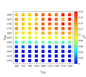
Figure 5.— Injection/reflection probability map as a function of the position of the upstream and downstream absorbing boundaries, UB and DB, respectively. The boundaries recede from the shock front moving leftwards on the UB-axis and upwards on the DB-axis.

The results are shown in Fig. 5, where the injection probability is plotted as a function of the position of UB and DB. The injection probability vanishes when DB is immediately downstream of the shock (lowest row in the probability grid), since all the trajectories are recorded at the boundary as soon as they cross the shock front. When DB recedes from the shock (moving upwards in the grid) the injection probability increases since more and more electrons have the chance to be deflected into the upstream. On the other hand, when UB is immediately upstream of the shock front, the reflection probability is maximum (for a fixed position of DB), since all the trajectories reflected upstream are registered as soon as they reach UB. When UB recedes from the shock (moving leftwards in the grid), the injection probability decreases since some of the trajectories can be further deflected into the downstream by the turbulent magnetic field in the precursor. The value of the injection probability reaches an almost constant value when DB is sufficiently far away from the shock and UB is upstream of the leading edge of the precursor, indicating that an accurate estimate of the asymptotic value has been reached. For the simulation described in Sect. 2, we find a reflection probability of $P_{\textrm{inj}}\sim 12\%$. The spectra of transmitted (blue, measured at the downstream edge of the simulation box) and reflected (red, measured at the upstream edge of the simulation box) electrons is shown in Fig. 6. The transmitted spectrum is plotted in the frame of reference computed from the Rankine-Hugoniot conditions as corresponding to that in which the downstream plasma would be at rest, if the electromagnetic fields have been completely annihilated (the “DRF”), whereas the spectrum of reflected particles is expressed in the URF.

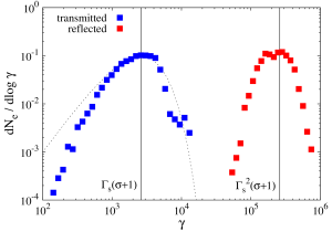
Figure 6.— Energy spectrum of test electrons transmitted (blue points) and reflected (red points) measured at the TS. The spectrum of transmitted particles is expressed in DRF, whereas the spectrum of reflected particles is expressed in the URF. The black dotted line represents a relativistic Maxwellian peaked at $\Gamma_{\textrm{s}}(\sigma+1)$. Both spectra are normalized to the number of trajectories recorded at the related boundary.

The spectrum of transmitted electrons resembles a relativistic Maxwellian, $M(\gamma)\propto\gamma\sqrt{\gamma^{2}-1}\,\textrm{exp}(-\gamma/\Delta\gamma)$, shown, for comparison as a black dotted line. This is in agreement with the results of Sironi & Spitkovsky (2011) and Teraki et al. (2015), who studied acceleration in the driven magnetic reconnection and in the superluminal regimes, respectively. The peak energy of the distribution is $\Gamma_{\textrm{s}}(\sigma+1)$, shown in Fig. 6 by the leftmost vertical black solid line, which means that in the electromagnetic precursor the electron energy increases on average by a factor of $\sigma$, as expected for complete dissipation of the Poynting flux. As for the spectrum of electrons upstream, the average energy is $\Gamma_{\textrm{s}}^{2}(\sigma+1)$, as expressed in the URF. This energy value is represented by the rightmost vertical black solid line in Fig. 6. The fact that during the first shock encounter the energy gain is $\propto\Gamma_{\textrm{s}}^{2}$ is well-known (e.g., Vietri, 1995; Gallant & Achterberg, 1999; Achterberg et al., 2001). However, here we show that the electromagnetically modified shock is able to energize the particles by an extra factor of $\sigma$ due to the dissipation of the magnetic field. The spectrum of reflected electrons in the URF is narrower than that of transmitted electrons in the DRF. In the URF, the angular distribution of reflected electrons is strongly peaked about the direction anti-parallel to the shock normal. We find that these results are insensitive to the period of the ensemble of snapshots folded to integrate the test electron trajectories, and have presented the results for the benchmark value $\tau=1000$. Furthermore, the reflection probability map and particle spectra are not sensitive to the injection prescription (1 or 2).

4. Monte Carlo simulations

In the idealized model of the pulsar wind as a magnetic shear, electrons that escape across the boundaries of our simulation box that encloses the TS shock are lost, in the sense that their trajectories never return to the box. In a more realistic picture, however, the incoming wave and the downstream plasma will contain magnetic irregularities, such as Alfvén waves or turbulence generated by the escaping particles themselves, which can perturb these trajectories. The realization that this process leads to particle acceleration underlies the theories of diffusive shock acceleration at non-relativistic shocks as well as the corresponding (but non-diffusive) process at relativistic shocks (for introductory reviews, see Drury, 1983; Kirk & Duffy, 1999). This process is thought to be suppressed at perpendicular, relativistic shocks (e.g., Summerlin & Baring, 2012; Sironi et al., 2015), but has so far not been investigated for the case in which the upstream plasma contains a field with reversing polarity, such as the magnetic shear considered in the previous two sections. For this purpose, we adapt a well tried and tested Monte-Carlo (MC) technique, which assumes the trajectories are stochastically perturbed by a scattering process that causes diffusion of the direction of propagation, but does not change the particle energy. Our method is equivalent to that of Summerlin & Baring (2012) in the limit of small-angle scattering; a recent implementation can be found in Takamoto & Kirk (2015).

At each time step, the particle momentum is advanced with an explicit first-order Euler’s scheme (Achterberg & Krülls, 1992). This is done in the upstream plasma according to the equations of motion in the unperturbed magnetic shear wave (Eqs. 1 and 2), whereas, in the downstream plasma, rectilinear motion is assumed, since the ambient fields vanish according to the two-fluid simulations in Sect. 2. Subsequently, a new direction of motion is randomly chosen in a cone of small aperture $\delta\theta_{\textrm{max}}$ about the previous direction, with a uniform distribution in the interval $[0:\delta\theta_{\textrm{max}}]$. The aperture, combined with the time-step $\Delta t$, sets the diffusion properties of the plasma which can be expressed as a scattering length

$$L_{\textrm{scat}}=\frac{6c}{\delta\theta_{\textrm{max}}^{2}/\Delta t}$$ (3)

which is the length-scale over which a particle is, on average, deflected by an angle $\pi/2$ by the magnetic turbulence, and not by the ambient field. The scattering length is a physical quantity, whose ratio to the wavelength of the shear in the upstream plasma determines the physics of acceleration. On the other hand, both $\Delta t$ and $\delta\theta_{\rm max}$ are artificial quantities introduced by the discretization procedure. For each simulation, we choose them to be sufficiently small and independent of particle energy. This implies that $L_{\rm scat}$ is also independent of particle energy, in contrast with the simulations of, for example, Summerlin & Baring (2012). We discuss this aspect in more detail below.

Each trajectory is initialized at the “shock front”, which corresponds to the upstream boundary of the two-fluid simulation, with momentum directed along the shock normal into the upstream and with $\gamma\gg\Gamma_{\textrm{s}}$. Upon returning to this boundary (which is fixed in the SRF), the Lorentz factor $\overline{\gamma}$ is unchanged, but the corresponding quantity in the SRF is larger. Using the test-particle integration technique described in Sect. 3, we find that particles re-entering the TS with such high Lorentz factors have a negligible probability for reflection — they pass through the simulation box with no change in Lorentz factor and remain essentially undeflected. Therefore, the MC code picks up the trajectory as it emerges on the downstream side of the TS with Lorentz factor and direction given by a Lorentz boost to the DRF, and follows it until it either returns and recrosses the TS, or reaches a boundary placed a fixed distance $d_{\textrm{abs}}$ downstream. We performed a series of tests on the position of this boundary, and selected $500\,\widetilde{L}_{\textrm{scat}}$, the minimum value for which the results showed no sensitivity. We denote by a tilde quantities measured in the DRF.

An important aspect of the simulations is the choice of $\delta\theta_{\textrm{max}}$. Electrons entering the upstream region are restricted to a cone $\overline{\mu}<-\beta_{\textrm{s}}$, where $\mu$ ($\overline{\mu}$) is the cosine of the angle between the shock normal and the particle momentum vector (and not the pitch-angle) in the SRF (URF). This defines a small angle

$$\sin\theta_{\textrm{c}}=\sqrt{1-{\beta}_{\textrm{s}}^{2}}=1/\Gamma_{\textrm{s}}\sim\theta_{\textrm{c}}$$ (4)

on which scale the angular distribution function of the particles is expected to show structure, when viewed in the URF. As mentioned above, here we use this MC technique to describe the process of diffusion in angle, which is represented in the transport equation by a Fokker-Planck operator (see e.g., Kirk & Duffy, 1999; Takamoto & Kirk, 2015). Thus, in order to simulate diffusion in direction accurately and to resolve the structures of the angular distribution, it is necessary to ensure that $\delta\theta_{\textrm{max}}\ll\theta_{\textrm{c}}$.

In contrast to non-relativistic shocks, particles that cross into the downstream region of the relativistic TS have a substantial probability of escaping over the downstream boundary. To compensate for this, and thereby minimize the effects of Poisson noise on the results, we implement a particle splitting method. Every time an electron completes five cycles (upstream-downstream-upstream), we use its momentum as the initial conditions for $N$ daughter particles ($N=10$–$50$), each of which is given a statistical weight $w_{\textrm{stat}}=1/N$ and is evolved independently.

We record the Lorentz factor and angle $\cos^{-1}\mu$ at all shock crossings for particles that have performed more than five cycles. From this, we construct the asymptotic (high-energy) particle distributions, averaged over the azimuthal angle: $f(\gamma,\mu)\propto\gamma^{-s+2}g(\mu)$, and extract the dependence on the polar angle $g(\mu)$ and the index $s$.

We have performed tests of our MC implementation for parallel shocks (or, equivalently, those in which there is no ordered magnetic field), and find good agreement between our results on the angular distribution and spectrum of accelerated particles and those of previous work (Kirk et al., 2000; Achterberg et al., 2001), for a wide range of shock speeds, ${\Gamma}_{\textrm{s}}{\beta}_{\textrm{s}}=10^{-1}$–$10^{3}$.

In the case of the pulsar TS, we expect the level of turbulence outside of the region simulated by the two-fluid code to be much smaller than that inside it, and so restrict ourselves to upstream scattering lengths that are longer than the wavelength of the magnetic shear wave ($\overline{L}_{\textrm{scat}}=10^{3}\,\overline{\lambda}$ for regime I, and $\overline{L}_{\textrm{scat}}=10^{2}\,\overline{\lambda}$ for regime II, see below). Downstream, there is no corresponding restriction, since the ordered field is assumed to be completely dissipated in the precursor-TS structure.

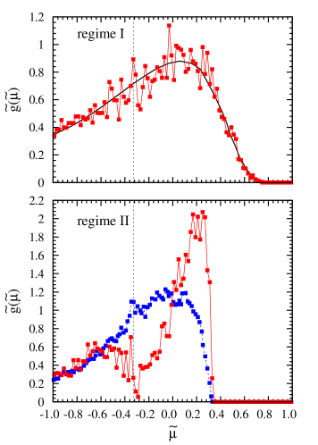
Figure 7.— Angular distribution expressed in the DRF for electrons accelerated at the pulsar wind TS ($\Gamma_{\textrm{s}}\beta_{\textrm{s}}=100$) in regime I (red, upper panel) in comparison with pure scattering at relativistic shock (black, eigenfunction method Kirk et al., 2000), and in regime II (red, lower panel) in comparison with regular magnetic field deflection (blue, numerical simulations, Achterberg et al., 2001).

In this case, our MC results show that electron acceleration proceeds in two distinct regimes, dictated by the relative magnitude of the wavelength of the stripes $\overline{\lambda}$ and of the electron gyro-radius $\overline{r}_{\textrm{g}}$. In the first — regime I — the gyro radius is large compared to the wavelength of the shear. This condition is automatically satisfied by the population of test particles depicted in Fig. 6. In the second — regime II — the gyro radius of accelerated particles is small compared to the wavelength of the magnetic shear wave. This regime corresponds to the situation with driven reconnection at the TS (Lyubarsky, 2003; Sironi & Spitkovsky, 2011), rather than the scenario presented in Sects. 2 and 3, and makes the implicit assumption that also in this case, particles can be injected into the relatively undisturbed upstream medium.

The angular distributions at the TS, as expressed in the DRF, are plotted for $\Gamma_{\textrm{s}}\beta_{\textrm{s}}=100$ in Fig. 7. The top panel shows regime I, and compares our results (red) with those obtained for an unmagnetized (or parallel) shock for $\Gamma_{\textrm{s}}\beta_{\textrm{s}}=10.0$ (black, eigenfunction method, Kirk et al., 2000). The bottom panel shows regime II, and compares our results (again in red) with those obtained for a magnetized perpendicular shock for $\Gamma_{\textrm{s}}\beta_{\textrm{s}}=100.0$ (blue, numerical simulations, Achterberg et al., 2001). The vertical black dotted line represents the value of the speed of the shock in DRF $\widetilde{\beta}_{\textrm{s}}$. This line divides electrons crossing from downstream to upstream on the left-hand side from electrons crossing from upstream to downstream on the right-hand side. In regime I, the wavelength of the magnetic shear is the shortest relevant scale. As a result, electrons are unmagnetized and scattering is the dominant source of particle deflection. We find a very good agreement between our results and the results of the eigenfunction method for $\Gamma_{\textrm{s}}\beta_{\textrm{s}}=10$ (which are indistinguishable from those of the asymptotic solution at $\Gamma_{\textrm{s}}\beta_{\textrm{s}}\to\infty$). The angular distribution is smooth, with a broad peak at $\widetilde{\mu}\sim 0.2$. The distribution extends to large values of $\widetilde{\mu}$ for electrons crossing from upstream to downstream. The corresponding spectral slope is $s=2.23\pm 0.01$ as expected for Fermi-like acceleration at an unmagnetized relativistic shock front.

Table 1Parameters of the simulation (including the energy range expressed in terms of particle gyro-radius) for electron acceleration at the pulsar wind TS ($\Gamma_{\textrm{s}}\beta_{\textrm{s}}=100.0$) for the scattering-dominated (I) and field-dominated (II) regimes.

regime	$\overline{\Delta t}$	$\overline{\delta\theta}_{\rm{max}}$	energy range	$s$
I	$10^{-6}$	$3\times{10^{-6}}$	$\overline{r}_{\textrm{g}}>30\overline{\lambda}$	$2.23\pm 0.01$
II	$10^{-5}$	$10^{-8}$	$10^{-8}\overline{\lambda}<\overline{r}_{\textrm{g}}<10^{-1}\overline{\lambda}$	$2.65\pm 0.03$

In regime II, the gyro-radius of accelerating electrons is smaller than the wavelength of the field. Consequently, the magnetic field in the wind is the dominant source of deflection. Electrons crossing the shock into the upstream medium essentially move into a uniform and static magnetic field (as assumed in the simulations represented by the blue curve) since these particles do not travel far enough into the magnetic pattern to experience the rotation of the magnetic field vector. However, the effect of the magnetic field of the shear wave differs from that of a static and uniform field, as shown in the bottom panel of Fig. 7, because in the former the magnetic field at the shock front rotates while the electron is engaged in an excursion downstream. The number of electrons grazing the pulsar wind termination shock, namely those with $\widetilde{\mu}\sim\widetilde{\beta}_{\textrm{s}}$, is strongly suppressed with respect to the uniform field case. Furthermore, the distribution is strongly peaked at $\widetilde{\mu}\sim 0.24$, while the angular distribution obtained in the other case is smoother and broader with a maximum at $\widetilde{\mu}\sim 0.0$. The resulting spectral index is $s=2.65\pm 0.03$, significantly different from the case of regular magnetic field deflection ($s=2.28\pm 0.01$, Achterberg et al., 2001). The parameters of these simulations are presented in Table 1.

On physical grounds, one expects that the scattering length $L_{\rm scat}$ should increase as the particle’s Lorentz factor grows, whereas, according to our definition in Eq. (3), it is constant. For the acceleration timescale, and for the particle energy spectrum in the transition region between regimes I and II, this is an important effect. However, since we are here concerned with the angular distribution and spectrum only within these regimes, and do not consider acceleration timescales, the chosen energy dependence of $L_{\rm scat}$ does not play a role.

5. Discussion

The two-fluid approach used by Amano & Kirk (2013) allows one to investigate the interaction between the pulsar wind and its termination shock in a scenario which is complementary to that of driven magnetic reconnection (e.g., Lyubarsky, 2003; Pétri & Lyubarsky, 2007; Sironi & Spitkovsky, 2011). Superluminal waves mediate this interaction when the frequency of the wave exceeds the proper plasma frequency ($\Omega>1$ in our notation), whereas a combination of an MHD shock and magnetic reconnection operates for $\Omega<1$, i.e., in a relatively high density regime (e.g., Sironi & Spitkovsky, 2011).

The breakout of the electromagnetic precursor due to the propagation of superluminal waves triggers the dissipation of the Poynting flux of the incoming wind, which starts at the leading edge of the precursor, well upstream of the main compression, and proceeds almost to completion, as illustrated in the bottom panels of Figs. 1 and 2. This mechanism creates a region of turbulent electromagnetic fields where low frequency superluminal waves can propagate and interact with the shear wave ahead of an essentially hydrodynamic sub-shock. The turbulent region is effective in energizing the electrons carried along with the wind, causing a sizeable fraction of them to be reflected after crossing the sub-shock. Upstream of the leading edge of the precursor the incoming plasma is still perturbed, most likely because of the propagation of high frequency superluminal waves, but there is only limited dissipation of the Poynting flux. The test-particle approach used here shows that electrons decoupled from the background plasma gain less than $1\%$ of their final energy in this region. This is due to the presence of a small electric field in the frame comoving with the electron-positron plasma. This heats and compresses the background plasma. On the other hand, test-particles gain momentum in the transverse plane, as shown in the bottom panel of Fig. 4. Since the electric field is perpendicular to the magnetic field, electrons acquire a small component of momentum in the transverse plane perpendicular to the magnetic field and start gyrating about the local magnetic field line. This causes the “bouncing”pattern of the parallel momentum (red) in the bottom panel of Fig. 4, where the peaks are due to motion parallel and anti-parallel to the $x$-axis. In the precursor, the net electric field in the comoving frame grows substantially, and electrons are accelerated in the direction perpendicular to the bulk motion by a non-MHD electric field arising in the interaction between the superluminal wave and the incoming shear wave (see Amano & Kirk, 2013, for a discussion on non-MHD fields in the two-fluid simulation). The parallel momentum can either increase (as for trajectory 4) or decrease according to the phase of the gyration when the electron enters the precursor. We stress that in Figs. 2-4, the black dashed line represents the average position of the leading edge of the precursor which is subjected to small fluctuations over the simulated time frame. Thus, the energy increase associated with the electron entering the precursor region can occur slightly upstream or downstream of the line depicted in the plots.

Even though the precursor is very turbulent, only the electromagnetic fields that survive downstream of the sub-shock are able to cause the first reversal of the electron trajectory (change of the sign of $\beta_{x}$) and turn trajectories around towards the upstream. This is illustrated by the sample of trajectories plotted in Fig. 3 and holds true for all of the several thousand test-particle trajectories we have examined.

We find an asymptotic value of the reflection probability at the TS in a striped wind (obtained for boundaries far from the sub-shock) of $P_{\textrm{inj}}\sim 12\%$, which is close to that found for parallel shocks using MC techniques (Bednarz & Ostrowski, 1999; Achterberg et al., 2001). This implies that electrons are injected into a subsequent, first-order Fermi process with comparable efficiency in the two cases, despite the fact that a striped wind requires particles to be boosted in energy before they can be reflected.

The spectrum of test electrons downstream of the shock resembles a relativistic Maxwellian peaked at $\sim\sigma\Gamma$, close to that expected for complete dissipation of the wave magnetization into test particles. This resembles the high density regime, where magnetic reconnection is expected to accelerate particles to a similar energy (Kirk, 2004; Kagan et al., 2015; Uzdensky, 2016). However, the dissipation of the magnetic field at the wind TS is not sufficient in itself to accelerate electrons into the power-law spectrum required to explain the observations of PWNe, which requires an additional acceleration mechanism.

The first-order Fermi process provides a possible scenario for this mechanism in the equatorial region of the TS in PWNe. The acceleration regime is determined by the size of the gyro-radius of the electron in comparison with the wavelength of the shear wave, or, in other words, of the wavelength of the stripes in the pulsar wind.

If $\overline{r}_{\textrm{g}}\gg\overline{\lambda}$, particles only perform a partial gyration about the magnetic field line (as seen in URF) before encountering the opposite phase of the magnetic shear wave and gyrating in the opposite direction. In this case, the variation of $\overline{\mu}$ during the partial orbit (electrons are confined into a cone $\overline{\mu}<-\beta_{\textrm{s}}$ upon entering the upstream region, see Sect. 4) is not sufficient for the shock front to overcome the particle. This result was already suggested by our test-particle simulation, where electrons travelling upstream of the leading edge of the precursor in the direction anti-parallel to the wind are always recorded at the upstream absorbing boundary. In regime I, the magnetic field is unimportant and only scattering off magnetic turbulence can provide the deflection necessary for the shock to overcome the electron (scattering-dominated regime). Regime I applies as long as the magnetic field is unable to provide the necessary deflection for electrons to cross the shock for the subsequent excursion in the downstream region. Consequently, the magnetic field is irrelevant for the acceleration process for

$$\frac{\overline{\lambda}}{\overline{r}_{\textrm{g}}}<\theta_{\textrm{c}}\,.$$ (5)

For electrons reflected at TS in our test-particle approach, this condition translates to

$$\overline{\gamma}>2\pi\sqrt{\sigma_{0}}\Gamma_{\textrm{s}}^{2}/\Omega$$ (6)

which is automatically satisfied for the majority of reflected particles, since these have $\overline{\gamma}\sim\sigma_{0}\Gamma_{\textrm{s}}^{2}$, and in this regime $\Omega\sqrt{\sigma_{0}}>1$. Thus, under pulsar wind conditions, although the upstream plasma is highly magnetized, the equatorial section of TS acts as an unmagnetized relativistic shock, producing the angular distribution and the power-law spectral index characteristic of first-order Fermi acceleration at unmagnetized relativistic shock fronts.

The second acceleration regime found in our MC approach (regime II, field-dominated) applies when Eq. (5) is not satisfied. This would require injection of particles in the upstream with $\overline{r}_{\textrm{g}}\ll\overline{\lambda}$, at odds with the results of Sect. 3. Assuming that such an injection mechanism can be provided by another mechanism, such as reconnection, the trajectory which enters the upstream is, nevertheless, bound to a specific field line which drives it back towards the shock. As seen in the URF, the electron again performs only a partial gyration about the field line. Since the shock is highly relativistic, it overruns the electrons soon after the condition $\overline{\mu}<-\beta_{\textrm{s}}$ is met, and prevents them from acquiring a large deflection. Therefore, the resulting angular distribution, which is plotted in the bottom panel of Fig. 7, shows almost no particles with $\widetilde{\mu}>0.4$. In addition, the number of electrons grazing the shock and accumulating at $\widetilde{\mu}=-0.33$ is suppressed in this case in comparison with the uniform magnetic field case (blue curve in the bottom panel of Fig. 7). In a uniform field, electrons moving parallel to the shock front ($\mu\sim 0$) and to the magnetic field in the upstream which perform very short excursions downstream (namely with little variation of $\mu$) are basically “bound”to the magnetic field line upstream. These electrons cross the shock multiple times (with very little energy gain at each cycle) and generate many shock crossing events with $\widetilde{\mu}\sim-\widetilde{\beta}_{\textrm{s}}$ in our plot. Such trajectories are absent in the case of a shear wave. In fact, during an excursion downstream, the orientation of the upstream field at the shock front changes and trajectories that return to the shock can suffer a very large change in pitch angle. This increases the average upstream excursion time and shifts the peak of the distribution of particles crossing the shock from upstream to downstream to larger values of $\widetilde{\mu}$. The larger average deflection upon returning to the shock leads to a larger average energy gain, but also to an increased escape probability. As a result, the spectrum of particles accelerated at a shear wave in regime II is softer than that of particles accelerated in a uniform field.

Comparing the two regimes we note that magnetic dissipation produces a Maxwellian spectrum in regime I, (as noted in Sect. 3), whereas regime II (driven reconnection) produces a power-law spectrum with a relatively hard $s\sim 1.5$ spectrum for $\gamma\ll\sigma_{0}\Gamma_{\textrm{s}}$ up to a cut-off (Sironi & Spitkovsky, 2011). In principle, the different signatures of acceleration contained in the angular distributions and, more importantly, in the energy spectra can be used to discriminate between the dissipation mechanisms that operate in the proximity of the TS. We stress that our conclusions apply only in the equatorial region of the pulsar wind TS, where the magnetic field averaged over the wavelength of the stripes is small. At higher latitudes, Fermi-type acceleration is inhibited by the large non-oscillating component of the magnetic field, which advects electrons away from the shock, quenching the acceleration process.

6. Conclusions

The relativistic shock front terminating the striped wind emitted by a pulsar in the equatorial region acts as an effectively unmagnetized shock. Electrons and positrons accelerated at this location have an angular distribution and a power-law spectral index consistent with the predictions of first-order Fermi acceleration at parallel, relativistic shocks.

We have used a combination of two-fluid, test-particle and Monte Carlo simulations to investigate electron acceleration at the termination shock in PWNe. The two-fluid simulations provide a representation of the turbulent electromagnetic fields in the proximity of the shock, capturing the process of dissipation of the magnetic field in the stripes of the wind and the formation of an electromagnetic precursor. We have shown that test-particle electrons propagating in the precursor increase their energy on average by a factor of $\sim\sigma_{0}$, as expected for almost complete dissipation of the Poynting flux at the TS. These particles form a relativistic Maxwell-like distribution peaked at $\sigma\Gamma_{\textrm{s}}$ in the downstream of the shock. A fraction $P_{\textrm{inj}}\sim 12\%$ of the incoming electrons is reflected upstream, forming a population of particles available for further acceleration. We have shown that subsequent stochastic acceleration at the shock can operate in two regimes. These are scattering- or field-dominated, according to the relative magnitude of the electron gyro-radius and wavelength of the stripes. Since, in pulsar wind environments the wavelength of the stripes is always the smallest relevant length-scale, the acceleration is likely to proceed in the scattering-dominated regime (regime I). The resulting angular distribution and spectral index $s=2.23\pm 0.01$ are similar to those obtained for Fermi acceleration at relativistic and unmagnetized shocks (when radiation losses are neglected). Interestingly, this slope is very close to the that needed to explain the TeV emission from the Crab. The field-dominated regime (regime II) corresponds to acceleration in driven magnetic reconnection and produces a softer spectrum of slope $s=2.65\pm 0.03$. However, this regime requires a different injection mechanism, which we do not discuss in this paper.

Finally, although we discuss our results in the context of PWNe, they may also be relevant to other sources that contain relativistic, magnetically dominated flows, such as AGNs or GRBs.

References

- Achterberg et al. (2001) Achterberg, A., Gallant, Y. A., Kirk, J. G., & Guthmann, A. W. 2001, MNRAS, 328, 393
- Achterberg & Krülls (1992) Achterberg, A., & Krülls, W. M. 1992, A&A, 265, L13
- Amano & Kirk (2013) Amano, T., & Kirk, J. G. 2013, ApJ, 770, 18
- Amato (2014) Amato, E. 2014, IJMPS, 28, 1460160
- Arka & Kirk (2012) Arka, I., & Kirk, J. G. 2012, ApJ, 745, 108
- Arons (2012) Arons, J. 2012, Space Sci. Rev., 173, 341
- Barkov & Komissarov (2016) Barkov, M. V., & Komissarov, S. S. 2016, MNRAS, 458, 1939
- Baty et al. (2013) Baty, H., Petri, J., & Zenitani, S. 2013, MNRAS, 436, L20
- Bednarz & Ostrowski (1998) Bednarz, J., & Ostrowski, M. 1998, Physical Review Letters, 80, 3911
- Bednarz & Ostrowski (1999) —. 1999, MNRAS, 310, L11
- Begelman & Kirk (1990) Begelman, M. C., & Kirk, J. G. 1990, ApJ, 353, 66
- Cerutti et al. (2016) Cerutti, B., Philippov, A. A., & Spitkovsky, A. 2016, MNRAS, 457, 2401
- Coroniti (1990) Coroniti, F. V. 1990, ApJ, 349, 538
- Drury (1983) Drury, L. O. 1983, Reports on Progress in Physics, 46, 973
- Gallant & Achterberg (1999) Gallant, Y. A., & Achterberg, A. 1999, MNRAS, 305, L6
- Kagan et al. (2015) Kagan, D., Sironi, L., Cerutti, B., & Giannios, D. 2015, Space Sci. Rev., 191, 545
- Kennel & Coroniti (1984) Kennel, C. F., & Coroniti, F. V. 1984, ApJ, 283, 694
- Kirk (2004) Kirk, J. G. 2004, Physical Review Letters, 92, 181101
- Kirk et al. (2009a) Kirk, J. G., Bell, A. R., & Arka, I. 2009a, PPCF, 51, 085008
- Kirk & Duffy (1999) Kirk, J. G., & Duffy, P. 1999, JPhG, 25, 163
- Kirk et al. (2000) Kirk, J. G., Guthmann, A. W., Gallant, Y. A., & Achterberg, A. 2000, ApJ, 542, 235
- Kirk et al. (2009b) Kirk, J. G., Lyubarsky, Y., & Petri, J. 2009b, in Astrophys. Space. Sci. Lib., Vol. 357, Astrophys. Space. Sci. Lib., ed. W. Becker, 421
- Kirk & Skjæraasen (2003) Kirk, J. G., & Skjæraasen, O. 2003, ApJ, 591, 366
- Lyubarsky & Kirk (2001) Lyubarsky, Y., & Kirk, J. G. 2001, ApJ, 547, 437
- Lyubarsky (2003) Lyubarsky, Y. E. 2003, MNRAS, 345, 153
- Michel (1991) Michel, F. C. 1991, Theory of neutron star magnetospheres (Chicago University Press)
- Mochol & Kirk (2013a) Mochol, I., & Kirk, J. G. 2013a, ApJ, 771, 53
- Mochol & Kirk (2013b) —. 2013b, ApJ, 776, 40
- Mochol & Pétri (2015) Mochol, I., & Pétri, J. 2015, MNRAS, 449, L51
- Olmi et al. (2015) Olmi, B., Del Zanna, L., Amato, E., & Bucciantini, N. 2015, MNRAS, 449, 3149
- Pétri & Lyubarsky (2007) Pétri, J., & Lyubarsky, Y. 2007, A&A, 473, 683
- Porth et al. (2014) Porth, O., Komissarov, S. S., & Keppens, R. 2014, MNRAS, 438, 278
- Press et al. (1986) Press, W. H., Flannery, B. P., & Teukolsky, S. A. 1986, Numerical recipes. The art of scientific computing (Cambridge: University Press, 1986)
- Sironi et al. (2015) Sironi, L., Keshet, U., & Lemoine, M. 2015, Space Sci. Rev., 191, 519
- Sironi & Spitkovsky (2009) Sironi, L., & Spitkovsky, A. 2009, ApJ, 698, 1523
- Sironi & Spitkovsky (2011) —. 2011, ApJ, 741, 39
- Summerlin & Baring (2012) Summerlin, E. J., & Baring, M. G. 2012, ApJ, 745, 63
- Takamoto & Kirk (2015) Takamoto, M., & Kirk, J. G. 2015, ApJ, 809, 29
- Takamoto et al. (2015) Takamoto, M., Pétri, J., & Baty, H. 2015, MNRAS, 454, 2972
- Tchekhovskoy et al. (2016) Tchekhovskoy, A., Philippov, A., & Spitkovsky, A. 2016, MNRAS, 457, 3384
- Teraki et al. (2015) Teraki, Y., Ito, H., & Nagataki, S. 2015, ApJ, 805, 138
- Uzdensky (2016) Uzdensky, D. A. 2016, in Astrophysics and Space Science Library, Vol. 427, Astrophysics and Space Science Library, ed. W. Gonzalez & E. Parker, 473
- Vietri (1995) Vietri, M. 1995, ApJ, 453, 883
- Zenitani et al. (2009) Zenitani, S., Hesse, M., & Klimas, A. 2009, ApJ, 696, 1385