A brief history of the introduction of generalized ensembles to Markov chain
Monte Carlo simulations

Abstract

The most efficient weights for Markov chain Monte Carlo calculations of physical observables are not necessarily those of the canonical ensemble. Generalized ensembles, which do not exist in nature but can be simulated on computers, lead often to a much faster convergence. In particular, they have been used for simulations of first order phase transitions and for simulations of complex systems in which conflicting constraints lead to a rugged free energy landscape. Starting off with the Metropolis algorithm and Hastings’ extension, I present a minireview which focuses on the explosive use of generalized ensembles in the early 1990s. Illustrations are given, which range from spin models to peptides.

1 Introduction

In this minireview I give a personal account of the birth of generalized ensemble simulations, which happened in the early 1990s. Though essential ideas go well back into the 1970s, they were not build on, but rediscovered around 1990. Later papers were often unaware of their predecessors. Nevertheless, I make here an attempt to present developments in a chronological order. Starting with the Metropolis algorithm, subsequent early work on the methodology, and Hastings’ extension to a general Markov chain Monte Carlo (MCMC) scheme, I come then to the introduction of generalized ensembles: Umbrella sampling and more than a decade later the almost simultaneous emergence of multicanonical (MUCA) ensembles, expanded ensembles and replica exchange simulations (parallel tempering).

My account of the last two methods remains rather sketchy as I was not involved into their development. My emphasis is on publications in which I participated and those which influenced my own work or crossed its path by one or another reason. No attempt of an “objective” overview or covering the field beyond the early developments is made. So, my focus is on MUCA simulations for which calculations of interface tensions of first order phase transitions via Binder’s method were the point of departure. Subsequently, I discuss applications to spin glasses and peptides (small proteins) as examples of complex systems with conflicting constraints. Concerning the performance, it is outlined that even for first order phase transitions a residual exponential slowing down remains. Wang-Landau sampling is recommended for calculating the MUCA weights. Summary and conclusion are given in the final section.

2 Metropolis algorithm and Hastings’ extension

MCMC calculations started in earnest with the 1953 paper by Metropolis, Rosenbluth² and Teller² Met . In their own words: “A general method, suitable for fast computing machines, for investigating such properties as the equations of state for substances consisting of interacting molecules is described. The method consists of a modified Monte Carlo integration over configuration space.” It relies on calculating the change in energy $\triangle E$, which is caused by a stochastic move of a particle position: “If $\triangle E<0$, i.e., if the move would bring the system to a state of lower energy, we allow the move and put the particle in its new position. If $\triangle E>0$, we allow the move with probability $\exp(-\triangle E/kT)$; i.e., we take a random number $\xi_{3}$ between 0 and 1, and if $\xi_{3}<\exp(-\triangle E/kT)$, we move the particle to its new position. If $\xi_{3}>\exp(-\triangle E/kT)$, we return it to its old position. Then, whether the move has been allowed or not, i.e., whether we are in a different configuration or in the original configuration, we consider that we are in a new configuration for the purpose of taking our averages.”

Whether to count a configuration after a rejected move again or not caused some discussion at its time and may still be a stumbling block for newcomers. I remember that I found the false choice in a lattice gauge theory (LGT) Metropolis programs of a postdoc in the 1990s, who had been running them for quite while on supercomputers.

2.1 Notable early developments

In 1959 Salsburg et al. Sals made an attempt to calculate the partition function by MCMC using a method called in the modern language “reweighting”:

$$\exp(-\beta E)\ \to\ \exp(-\beta E-\triangle\beta E)=\exp(-\beta^{\prime}E)\,.$$ (1)

As noticed by the authors their method is restricted to very small lattices when one wants to cover the entire $\beta$ range from 0 to $\infty$ as needed for the partition function, because for a fixed, possibly large, statistics and away from critical points $\triangle\beta\sim 1/\sqrt{\rm V}$ ($V$ volume) holds for the admissible $\triangle\beta$ range.

In the next almost thirty years reweighting was several times forgotten and re-discovered (for instance, McDonald and Singer McDS used reweighting to evaluate physical quantities over a small range of temperatures) until finally the time was right and the MCMC community had grown large enough so that reweighting never became extinct again after the 1988 paper by Ferrenberg and Swendsen FS .

Continuing with the MCMC time line, in his 1963 article Glauber Glauber transcends the Metropolis dynamics by introducing the heatbath and other dynamical approaches for the Ising model.

2.2 Hastings

In Hastings own words Hastings : “A generalization of the sampling method introduced by Metropolis et al. (1953) is presented along with an exposition of the relevant theory, techniques of application and methods and difficulties of assessing the error in Monte Carlo estimates.” Unfortunately, the mathematician Hastings renamed everything the chemists and physicists had introduced before: “Equilibrium” to “stationary”, “detailed balance” to “reversibility” and “ergodicity” to “irreducibility”.

Instead of focusing on the Boltzmann distribution, Hastings constructs a Markov chain matrix $P$ with a general stationary distribution $\pi$. Following his paper, the matrix $P$ is made to satisfy the detailed balance (reversibility) condition

$$\pi_{i}\,p_{ij}=\pi_{j}\,p_{ji}$$ (2)

for all pairs of states $i$ and $j$. This property ensures that $\sum_{i}\pi_{i}p_{ij}=\pi_{j}$ for all $j$, and hence that $\pi$ is an equilibrium (stationary) distribution of $P$. Ergodicity (irreducibility) of $P$ must be checked in each specific application. For this it is only necessary that there is a positive probability of going from state $i$ to state $j$ in some finite number of transitions.

It is then assumed that $p_{ij}$ has the form

$$\pi_{i}\,p_{ij}=q_{ij}\,\alpha_{ij}\ (i\neq j)~{}~{}{\rm with}~{}~{}p_{ij}=1-\sum_{j\neq i}p_{ij}\,.$$ (3)

Here $Q=\{q_{ij}\}$ is the transition matrix of an arbitrary Markov chain on the states $0,1,\dots,S$ and $\alpha_{ij}$ is given by

$$\alpha_{ij}=\frac{s_{ij}}{1+(\pi_{i}q_{ij})/(\pi_{j}q_{ji})}\,,$$ (4)

where it is noticeable that the normalization of the distribution $\pi$ drops out. Metropolis updating $(s^{M}_{ij})$ is a special case:

$$s_{ij}^{M}=\cases{1+(\pi_{i}q_{ij})/(\pi_{j}q_{ji})\ {\rm for}\ (\pi_{j}q_{ji})/(\pi_{i}q_{ij})\geq 1\ \Rightarrow\ \alpha_{ij}^{M}=1\,,\cr 1+(\pi_{j}q_{ji})/(\pi_{i}q_{ij})\ {\rm for}\ (\pi_{j}q_{ji})/(\pi_{i}q_{ij})<1\ \Rightarrow\ \alpha_{ij}^{M}=(\pi_{j}q_{ji})/(\pi_{i}q_{ij})\,.}$$ (5)

It goes for $q_{ij}\neq q_{ji}$ sometimes under the name biased Metropolis updating. Requiring symmetry:

$$q_{ij}=q_{ji}~{}~{}\Rightarrow~{}~{}\alpha_{ij}^{M}=\cases{1~{}{\rm for}~{}\pi_{j}/\pi_{i}\geq 1\,,\cr\pi_{j}/\pi_{i}~{}{\rm for}~{}\pi_{j}/\pi_{i}<1\,,}$$ (6)

and assuming the Boltzmann distribution $\pi_{i}=\exp(-\beta E_{i})$, we obtain the original Metropolis algorithm back.

However, Hastings did not make progress in identifying suitable distributions $\pi$ for important applications and error estimates of MCMC simulations are nowadays much better under control BB04 . Besides, Hastings appeared to be unaware of Glauber’s earlier work Glauber generalizing the Metropolis approach.

3 Umbrella sampling

Until about 1990 the paradigm of MCMC calculations in statistical physics appeared to be that the use of Boltzmann weights will optimize the simulation. However, there had been notable exceptions.

Figure 1: Probability density $P(E)$, $E$ energy, for a umbrella sample (solid line) together with canonical probabilities at two temperatures, $T_{1}$ and $T_{2}$, as obtained by reweighting of the umbrella sample (sketched according to TV77 ).

Already in 1972 Valleau and Card VC72 used overlapping bridging distributions to estimate entropy and free energy by what they called “multistage sampling”. Nowadays we call this multi-histogram reweighting. Torrie and Valleau TV74 continued with estimation of free energies from distributions designed for this purpose. Patey and Valleau PV75 sampled ionic potentials with weights $w(r_{12})\,\exp(-U/kT)$, where the weighting functions $w(r_{12})$ was chosen to spread the sampling over a desired range. In 1977 this line of work culminated in the proposal of “Nonphysical Sampling Distributions in Monte Carlo Free-Energy Estimation: Umbrella Sampling” by Torrie and Valleau TV77 .

Markov chains, which sample these distributions, are special cases of Hastings framework, but the real problem is the engineering of sampling weights that work for a particular purpose. In any case, no reference to Hastings is given, though his Hastings and the Valleau et al. papers VC72 ; TV74 ; PV75 ; TV77 have in common to be products of Toronto University.

The basic idea of umbrella sampling is sketched in Fig. 1: The umbrella distribution is much broader than canonical distributions in its range, which are then not obtained by direct simulations, but by reweighting of a umbrella distribution. This leads us to the question “How to get the umbrella distribution in the first place?” and we find in the paper of Torrie and Valleau TV77 : “Superficially, the most serious limitation of the sampling techniques described here may appear to be the lack of a direct and straightforward way of determining the weighting function to use for a given problem. Instead $w({\bf q}^{N})$ must be determined by a trial-and-error procedure for each case, often beginning with the information available from the distribution in a very short Boltzmann-weighted experiment which is then broadened in stages through subsequent short test runs with successively greater bias of the sampling. What this rather inelegant procedure lacks aesthetically is more than compensated by the efficiency of the ultimate umbrella-sampling experiment.”

Umbrella sampling survived mainly in a niche of computational chemistry, e.g., Ch85 . But ten years later the conclusion by Lie and Scheraga LS88 was still: “The difficulty of finding such weighting factors has prevented wide applications of umbrella sampling”.

What is really gained by using umbrella distributions instead of a series of canonical samples and possibly patching them? The documentation at its time remained rudimentary and gains appear to be no larger than, maybe, factors of 10 to 20. An exception is the improvement one can find in chapter 6.3 of the 1987 statistical mechanics book by Chandler Chandler . He considered a $20\times 20$ Ising model below the (critical) Curie temperature, where visitation of states with magnetization $m=0$ is a rare event. By patching 10 umbrella windows he can reach $m=0$ and sample configurations which are in canonical Boltzmann simulations suppressed by 6 to 7 orders of magnitude. Unfortunately, this impressive demonstration of the numerical method missed a physical focus. Naturally this would have been a calculation of the interface tension, known exactly since Onsager’s Onsager 1944 solution of the 2D Ising model. However, this requires Binder’s Bi82 relation (7), which is discussed in the next section (presumably Chandler was not aware of it).

Independently of Chandler, and unaware of umbrella sampling, Bhanot and collaborators Bh87 developed a similar method of patching microcanonical simulations, then defined as simulations restricted to some small energy range $E_{\min}\leq E\leq E_{\max}$, and applied it to a number of physical topics.

4 Multicanonical and other generalized ensembles

The spread of the multicanonical approach is an example of an interdisciplinary success story with unexpected turns of events. In 1988 Parisi et al. Pa88 claimed that the deconfining phase transition of SU(3) LGT is second order, what appeared rather weird, because a large number of previous publications had agreed on a weak first order transition. However, as this was Georgio Parisi, everyone felt obliged to take this very seriously and immediately, as well as over the subsequent years, a large number of papers appeared, including one by myself and collaborators BB90 , which all re-confirmed the first order nature of this transition.

This also stimulated work on simpler models than SU(3) LGT with the aim to develop better methods to identify first order transitions. Examples of simple systems with first order phase transitions are 2D and 3D Ising models below the Curie temperature for which the transition is at $h=0$ in an applied magnetic field and $q$-state Potts models for which there is a first order transition in the temperature ($q\geq 4$ in 2D, $q\geq 3$ in 3D required). One focus was on calculations of their interface tensions. In particular, Potvin and Rebbi PR89 as well as Kajanti et al. Ka89 , used the 7-state 2D Potts model as laboratory for a newly developed approach, which estimated the interface tension by driving half a lattice “adiabatically” from one phase into the other. Thomas Neuhaus and I stumbled in this context over Binder’s method for estimating interface tensions.

4.1 Binder’s method

Figure 2: Ising model with periodic boundary conditions below the Curie temperature: Order parameter (magnetization) distribution (qualitatively drawn after Ref. Bi82 ).

Figure 2 sketches the probability density of the magnetization $m$ for a 2D Ising model with periodic boundary conditions at a temperature below its critical and at external magnetic field $h=0$. For the interface tension $f^{s}$ Binder Bi82 derived the relation

$$f^{s}\ =\ \lim_{L\to\infty}f^{s}_{L}~{}~{}{\rm with}~{}~{}f^{s}_{L}\ =\ -\frac{1}{L^{(D-1)}}\,\ln\left(\frac{P^{\min}_{L}}{P^{\max}_{L}}\right)\,,$$ (7)

where $P^{\max}_{L}$ is the maximum and $P^{\min}_{L}$ the minimum of the probability density of the magnetization on a finite lattice of size $L^{D}$ with periodic boundary conditions. In case of the order-order transition of Fig. 2 at $h=0$ it is obvious that the probability density is symmetric in the magnetization $m$. For a temperature driven first order transition there is no such symmetry. The energy, instead of the magnetization, is recorded on the abscissa and it becomes part of the calculations to determine suitable pseudotransition temperatures $\beta_{t}(L)$.

On finite lattices $P^{\max}_{L}$ and $P^{\min}_{L}$ can be calculated by MCMC, but initial attempts Bi82 remained pitiful, because they were carried out in the canonical ensemble and estimates deteriorate then quickly with increasing lattice size as configurations for $P^{\min}_{L}$ are exponentially suppressed according to $P^{\min}_{L}\sim\exp\left(-f^{s}L^{D-1}\right)$. So, Binder’s method remained dormant for almost ten years.

4.2 Multicanonical ensemble

Figure 3: Reweighting of a MUCA simulation at the first order phase transition of the 2D 10-state Potts model to the canonical ensemble BN92 .

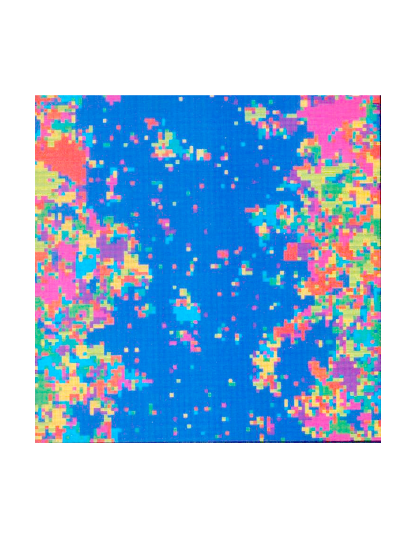
Figure 4: 2D 10-state Potts model: A configuration with disorder-order interfaces from the $P_{L}^{\min}$ configurations of the canonical ensemble.

For a temperature driven first order transition the MUCA approach BN91 ; BN92 calculates $P_{L}^{\min}$ by sampling no longer with Boltzmann weights but with the inverse number of states,

$$W(E)\ =\ {\rm const}/n(E)\,,$$ (8)

as weights. Subsequently, one reweights the thus obtained MUCA ensemble to the canonical ensemble at an effective transition temperature, $\beta_{t}(L)$, for which equal heights of the maxima of the spectral probability density are realized (equal weights have also been suggested BK92 ).

In contrast to umbrella sampling the MUCA weights are precisely defined, but in principle MUCA appears to suffer from the same shortcoming: The weights are a-priory unknown (in contrast to the Boltzmann weights). However, well defined target weights led to a clear focus on the problem of getting them. Especially, for the envisioned calculations of interface tensions weights can be obtained by finite size extrapolations from small to increasingly larger systems: For very small systems canonical simulations work and provide the starting point. Then one extrapolates weights for the next larger system, corrects them by simulation results from this system, proceeds to the next larger system, and so on.

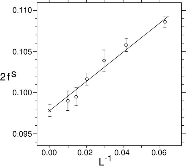
Figure 5: Extrapolation of the interface tension for the 2D 10-state Potts model BN92 .

Table 1: Interface tensions $f^{s}$ for some 2D Potts models.

$q$	MUCA JBK92 ; BN92	Potvin and Rebbi PR89	Exact (Borgs and Janke BJ92 )
7	0.0241 (10)	0.1886 (12)	0.020792$\dots$
10	0.09781 (75)	$-$	0.094701$\dots$

For the 2D 10-state Potts model lattices up to size $100^{2}$ were covered in this way. Figure 3 shows for a $70^{2}$ lattice the energy histogram obtained by using approximate MUCA weights and at the pseudotransition temperature the canonically reweighted histogram. Improvements by a factor $10^{5}$ over canonical simulations are easily achieved. Figure 4 gives an example of a configuration with interfaces as found for $P^{min}_{L}$ in the canonical ensemble. Equation (7) yields for each lattice size the effective interface tension and in Fig. 5 these estimates are extrapolated to the infinite volume result ($1/L\to 0$). The thus obtained $f^{s}$ is the second entry of the third row of Table 1.

However, there was a problem now: The MUCA estimate for the interface tension of the 2D 10-state Potts model is lower than this estimate for the 2D 7-state Potts model by Potvin and Rebbi PR89 , the third entry of the second row of Table 1 (Kajanti et al. Ka89 agree and give $2f^{s}\approx 0.2$ without error bar). As the strength of the 2D Potts model transitions increases with the number of states, this should be the other way round. The discrepancy was confirmed by a direct MUCA calculation of the 2D 7-state Potts model JBK92 for which $f^{s}$ is listed as the second entry of the second row of Table 1. What now? As nobody will easily admit that his or her numerical method does not work, an endless debate was looming. But:

4.3 Miracles happen (thanks to Borgs and Janke)

After the numerical results were published Borgs and Janke BJ92 realized, based on previous work by Buffenoir and Wallon BW92 and others, that there is actually an exact solution for the interface tension of 2D $q$-state Potts models. While numerical calculations tend to reproduce known exact results accurately, this was not so much the case for these previously unknown exact results, which are for the 2D 7-state and 10-state models collected in the 4th column of Table 1. The MUCA estimate for the 10-state Potts model agrees within less than 4%, but only within five sigma. For the 7-state model the MUCA estimate needs three error bars to include the exact value. However, this is very good when compared to the other numerical estimate for the 7-state model, which is an entire order of magnitude too large. So, due to the paper by Borgs and Janke the looming endless discussion was cut short (the interfaces are perceived as too stiff in the method of PR89 ; Ka89 ). Looking back, the controversy helped a lot to draw attention on MUCA simulations as a reliable method. Almost needless to say, once the exact results are known, the discrepancies with MUCA estimates can be resolved by applying more sophisticated fits BNB94 than the one of Fig. 5.

4.4 Other early multicanonical simulations and new horizons

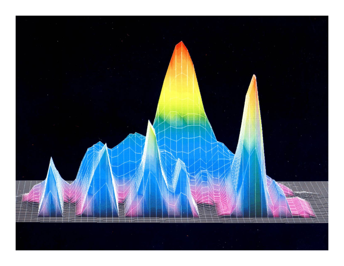
Figure 6: Probability densities of the magnetization for the 3D Ising model at a temperature below its critical value BHN93 .

Figure 7: Snapshot from a MUCA simulation of the 2D Edwards-Anderson Ising spin glass, which exhibits barriers in the overlap parameter BC92 .

Soon MUCA calculations were also carried out for the interface tensions of the order-order transitions of 2D and 3D Ising models below their critical temperatures and MUCA is in this application called multimagnetical (MUMA). The 2D case allows for comparison with Onsager’s Onsager exact result and MUMA calculations were well consistent BHN91 . This was certainly of interest when this paper was submitted in September 1991 and the controversy about the estimates for Potts models was still unsettled. However, due to the malice of some referees, which were finally overruled by the editor, the paper appeared only in January 1993. By then subsequent work BHN93 , which included estimates for 3D Ising model interface tensions, appeared almost simultaneously in print. Figure 7 shows the reweighted canonical probability densities of one of our MUMA simulations of the 3D Ising model and it is clear that an astronomically large improvement over canonical simulation is reached: Configurations for the minimum are sampled, which are suppressed by a factor of approximately $e^{-150}\approx 10^{-60}$ in the canonical ensemble.

Somewhat later extensions of the MUCA method to cluster algorithms, multibondic (MUBO) simulations, were introduced and studied by Janke and collaborators JK95 ; BJ07 .

Realizing the importance of the MUCA approach beyond first order phase transitions, Celik and I BC92 published in 1992 an application to complex systems with a rugged free energy landscape due to frustrated interactions: The 2D Edwards-Anderson Ising spin glass. By sampling with MUCA weights (8) one can move in and out of valleys and find their relative heights by connecting them through the disordered phase. This is illustrated in Fig. 7: The mountain in the background is sampled from configurations of the disordered high temperature phase and the MUCA updating process travels in and out of low temperature valleys (this is where the histogram entries are), which are separated by high barriers (means no histogram entries) in the probability density of the overlap parameter. Our spin glass investigations with MUCA went on for quite a while BCH and the final paper with Billoire and Janke BBJ was about overlap barriers in the 3D and 4D Edwards-Anderson Ising spin glass model. In contrast to first order phase transitions finite size extrapolations of the MUCA weights are not possible for spin glasses, because each replica is unique. So, Ref. BC92 introduced a recursive approach to estimate them. Progress has since then been achieved with respect to this and is shortly reviewed in section 4.7.

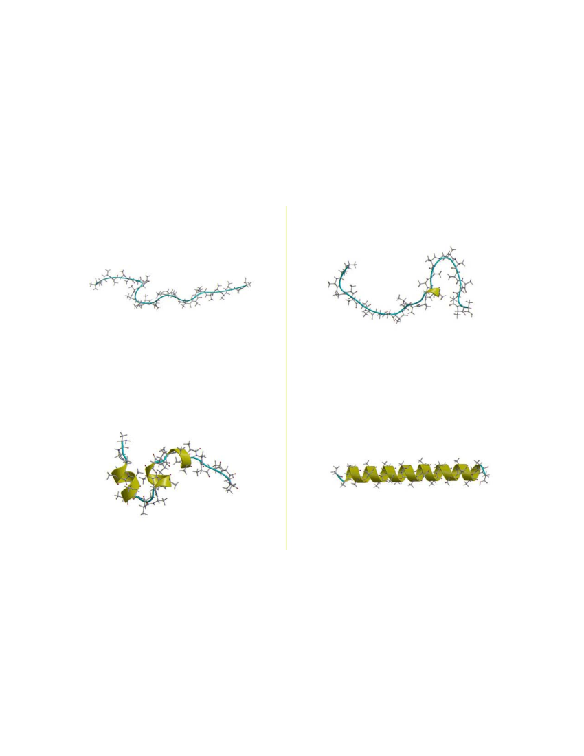
Figure 8: Configurations from folding of poly-alanine into its helix groundstate HO99a .

The concluding remarks in BC92 are: “The similarities of spin glasses to other problems with conflicting constraints suggest that MUCA simulations may be of value for a wide range of investigations: optimization problems like the traveling salesman, neural networks, protein folding, and others.” Hansmann and Okamoto made the application to small proteins reality HO93 . Figure 8 pictures the folding of poly-alanine configurations into their helix groundstates in a MUCA simulation that connects the native groundstate with a disordered initial configuration HO99a . Their review article HO99b coined the generic name “Generalized Ensembles” for MUCA ensembles, umbrella sampling, expanded ensembles and the replica exchange method.

4.5 Expanded ensembles and the replica exchange method

Expanded ensembles LM92 ; MP92 enlarge the configuration space by one or more additional variables. If this is the temperature, the method is also called “simulated tempering”. In the replica exchange method Ge91 ; HN96 several identical replica of the systems are simulated with parameter values chosen so that transitions between the replica, which are accepted according to the Metropolis method, become possible, i.e., have reasonable acceptance rates. This is a special case of the approach of Ref. SW86 , which was not focused enough to provide guidance for practical applications. The replica exchange method allows for easy parallelization, because the simulation of each replica is independent from that of the other replica and the exchanges requires only transfer of a few variables. See Ja08 for work by Janke and collaborators on this subject.

If the replica differ in the temperature variable, the replica exchange method is often called “parallel tempering” (PT), which should not be confused with simulated tempering. Presumably due to the easy use of many processors on supercomputers, PT has become quite popular, in particular for protein simulations to which it was introduced in Ref. Ha97 within the MCMC framework. However, in biophysics molecular dynamics (MD) simulations are most widely used. To them PT was adapted a few years later in Ref. SO99 .

That all these methods flourished since the early 1990s, and were not forgotten again, shows that by now the time was right to create a sufficiently large and sophisticated user community.

4.6 Performance of generalized ensemble simulations

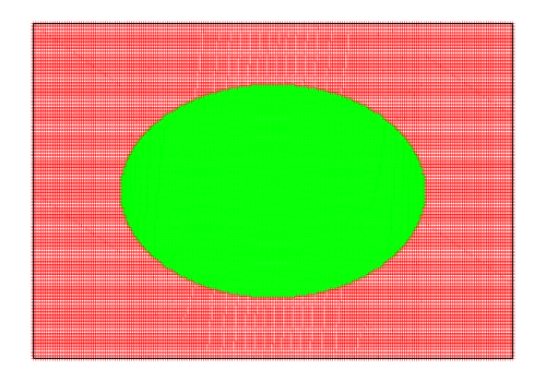
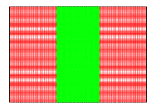
Figure 9: Energy optimized droplet versus percolated configuration as discussed in NH03 .

The number of steps a random walk (diffusive process) needs to bridge a distance $N$ is proportional to $N^{2}$. Therefore, the optimal performance of a MUCA simulation to bridge an extensive energy gap is proportional to $V^{2}$, where $V$ is the volume of the system. In the early work BN92 it was assumed that for first order transitions the performance would be close to this optimum, something like $V^{2.3}$ was consistent with the data. This turned out to be too optimistic. The slowing down is still exponential in system size $L$. Only the worst exponential, $\sim\exp\left(-f^{s}L^{D-1}\right)$, has been eliminated. The argument due to Neuhaus and Hager NH03 is illustrated in Fig. 9 for an order-order transition. The interface energy minimized shape for the green within the red phase is a droplet as long the green phase region is sufficiently small. However, once the green phase is sufficiently large, the optimal shape becomes the percolated green rectangle and transitions from the droplet to the rectangle have to go through exponentially suppressed configurations. This is an example of hidden barriers for which a good reweighting variable is difficult to identify. In practice the coefficient of this subleading exponential appears to be rather small, so that the diffusive process dominates the slowing down for some while and effectively a power law in $L$ is observed as long as the systems are not too large.

This argument does not apply directly to PT, because each replica is then simulated in the canonical ensemble. As a consequence rare configurations of free energy barriers like the one of the right side of Fig. 9 are in practice not sampled but at best jumped and it is wrong to use this method when one is interested in sampling barrier configurations. On the other hand, when one is interested in connecting distinct groundstate branches, like those of our spin glass Fig. 7, through the disordered phase, PT appears to be well suited.

4.7 Wang-Landau recursion and parallelization

Ever since BC92 recursions for MUCA weights received appropriate attention. The proposed schemes, like Be96 , relied on manipulations of additive histograms of the already covered energy ranges. This changed when Wang and Landau WL01 introduced a new sampling method that relies on a multiplicative instead of a additive recursion of weights:

$$\ln W(E)\ \to\ \ln W(E)-a\,,~{}~{}a>0\,,$$ (9)

whenever the (discrete) energy $E$ is sampled. Then $a\to a/2$ after a sufficiently flat histogram is obtained. Though proposed as a sampling method, in the MUCA context it is best used as a recursion where the weights get frozen once they are working estimates of the MUCA weights. Here “working estimate” means that the energy range of interest is cycled with the frozen weights (instead of getting stuck in part of that range). In tests, which I performed iterating the MUCA weights this way, it has turned out to be a robust way of getting working estimates within a small fraction of the CPU time needed for the subsequent calculation with fixed weights. So, there is little incentive to hunt for further improvement, although it is not finally settled whether additive recursions can do as well or even better (a poster Ja16 comparing Wang-Landau and MUCA recursions was presented at this conference).

With Bazavov BB09 I have worked out a straightforward implementation of the Wang-Landau recursion for the case of a continuous energy variable. The basic steps are:

1. Bin into histograms just large enough so that a single updating step cannot jump a bin.

2. Track the mean values within each bin.

3. Do not use constant weights over a bin, but interpolate logarithmic weights (9) weights linearly between mean values of neighbor bins.

The performance was as good as the one achieved in models with discrete energies.

For simulations on supercomputers parallelization is crucial. Here I like to point the reader towards two relatively recent papers. Massively parallel Wang-Landau sampling is discussed by Landau and collaborations in La13 and parallelization of MUCA simulations by Janke and collaborators in Ja13 .

5 Summary and conclusions

A message is that mastering simulational methods is not the trivial part of a physical, chemical or biophysical MCMC study. Astronomically large efficiency factors can float around between getting a simulation optimized or not. There have been hundreds of papers refining and improving the methods sketched here. Within this limited review I cannot follow up on them. An efficient way to track such investigations is to look for citations of the papers quoted here and work from there up to the latest developments.

Obviously, for a number of applications generalized ensembles allowed great leaps in the efficiency of MCMC simulations, but ultimately it is unavoidable that one reaches some limits where one is stuck again. The two main problems appear to me:

1. There are often hidden barriers and we have been unable to find reaction coordinates in which these barriers become explicit. Recommendation: Keep trying.

2. The optimal performance of the discussed methods is limited by the $V^{2}$ power law due to being a diffusive process. For large systems that can still be far too slow.

At second order phase transitions collective updating with cluster algorithms provides great improvements, but they have a rather limited applications range. Non-equilibrium simulations could be a way out if one could relate the generated configurations to those of canonical equilibrium ensembles. Putting in some dynamics into simulations by combinations of MCMC with MD may help. Most important, we are awaiting the not yet existing ideas of the next generation of computational physicists.

Acknowledgments: I would like to thank Martin Weigel and the other organizers for inviting me to Wolfhard’s belated birthday party.

References

- (1) N. Metropolis, A.W. Rosenbluth, M.N. Rosenbluth, A.H. Teller and E. Teller, J. Chem. Phys. 21, (1953) 1087-1092
- (2) Z.W. Salsburg, J.D. Jacobson, W.S. Fickett and W.W. Wood, J. Chem. Phys. 30, (1959) 65-72
- (3) I.R. McDonald and K. Singer, Disc. Faraday Soc. 43, (1967) 40-49
- (4) A.M. Ferrenberg and R.H. Swendsen, Phys. Rev. Lett. 61, (1988) 2635-2638; 63, (1988) 1658
- (5) R.J. Glauber, J. Math. Phys. 4, (1963) 294-307
- (6) W.K. Hastings, Biometrika 57, (1970) 97-109
- (7) B.A. Berg, Markov chain Monte Carlo simulations and their statistical analysis (World Scientific, 2004)
- (8) J.P. Valleau and D.N. Card, J. Chem. Phys. 57, (1972) 5457-5462
- (9) G.M. Torrie and J.P. Valleau, Chem. Phys. Lett. 28, (1974) 578-581
- (10) G.N. Patey and J.P. Valleau, J. Chem. Phys. 63, (1975) 2334-2339
- (11) G.M. Torrie and J.P. Valleau, J. Comp. Phys. 23, (1977) 187-199
- (12) J. Chandrasekar, S.F. Smith and W.K. Jorgensen, J. Am. Chem. Soc. 107, (1985) 154-163
- (13) Z. Lie and H.A. Scheraga, J. Mol. Struct. (Theochem) 179, (1978) 333-352
- (14) D. Chandler, Introduction to Modern Statistical Mechanics, (Oxford University Press, 1987)
- (15) L. Onsager, Phys. Rev. 65, (1944) 117-149
- (16) K. Binder, Phys. Rev. A 25, (1982) 1699-1709
- (17) G. Bhanot, R. Salvador, S. Black, P. Carter and R. Toral, Phys. Rev. Lett. 59, (1987) 803-806 and references therein
- (18) G. Parisi et al., Phys. Rev. Lett. 61, (1988) 1545-1548
- (19) N.A. Alves, B.A. Berg and S. Sanielevici, Phys. Rev. Lett. 64, (1990) 3107-3110
- (20) J. Potvin and C. Rebbi, Phys. Rev. Lett. 62, (1989) 3062-3065
- (21) K. Kajanti, L. Kärkkäinen and K. Rummukainen, Phys. Lett. B 223, (1989) 213-217
- (22) B.A. Berg and T. Neuhaus, Phys. Lett. B 267, (1991) 249-253
- (23) B.A. Berg and T. Neuhaus, Phys. Rev. Lett. 68, (1992) 9-12
- (24) C. Borgs and S. Kappler, Phys. Lett. A 171, (1992) 37-42
- (25) W. Janke, B.A. Berg and M. Katoot, Nucl. Phys. B 382, (1992) 649-661
- (26) C. Borgs and W. Janke, J. Phys. I France 2, (1992) 2011-2018
- (27) E. Buffenoir and S. Wallon, Saclay preprint SPHT/92-077
- (28) A. Billoire, T. Neuhaus and B.A. Berg, Nucl. Phys. B 413, (1994) 795-812
- (29) B.A. Berg, U. Hansmann and T. Neuhaus, Phys. Rev. B 47, (1993) 497-501
- (30) B.A. Berg, U. Hansmann and T. Neuhaus, Z. Phys. B 90, (1993) 229-239
- (31) W. Janke and S. Kappler, Phys. Rev. Lett. 74, (1995) 212-215
- (32) B.A. Berg and W. Janke, Phys. Rev. Lett. 98, (2007) 040602.
- (33) B.A. Berg and T. Celik, Phys. Rev. Lett. 69, (1992) 2292-2295
- (34) B.A. Berg, T. Celik and U. Hansmann, Phys. Rev. B 50, (1994) 16444-16452
- (35) B.A. Berg, A. Billoire and W. Janke, Phys. Rev. B 61, (2000) 12143-12150
- (36) U. Hansmann and Y. Okamoto, J. Comp. Chem. 14, (1993) 1333-1338
- (37) U. Hansmann and Y. Okamoto, J. Chem. Phys. 110, (1999) 1267-1276; Erratum 111, (1999) 1339
- (38) U. Hansmann and Y. Okamoto, Ann. Rev. Comp. Phys. (edited by D. Stauffer) VI, (World Scientific 1999) 129-157
- (39) A.P. Lyubartsev, A.A. Martsinovski, S.V. Shevkanov and P.N. Vorontsov-Velyaminov, J. Chem. Phys. 96, (1992) 1776–1783
- (40) E. Marinari and G. Parisi, Europhys. Lett. 19, (1992) 451-458
- (41) G.J. Geyer in Computing Science and Statistics, Proceedings of the 23rd Symposium on the Interface (edited by E.M. Keramidas and S.M. Kaufman), (1991) Interface Foundation, Fairfax, VA, 156–163
- (42) K. Hukusima and K. Nemoto, J. Phys. Soc. Japan 65, (1996) 1604–1608
- (43) R.H. Swendsen and J.-S. Wang, Phys. Rev. Lett. 57, (1986) 2607–2609
- (44) U.H. Hansmann, Chem. Phys. Lett. 281, (1997) 140-150
- (45) E. Bittner, A. Nußbaumer and W. Janke, Phys. Rev. Lett. 101, (2008) 130603
- (46) Y. Sugita and Y. Okamoto, Chem. Phys. Lett. 314, (1999) 141-151
- (47) T. Neuhaus and J.S. Hager, J. Stat. Phys. 113, (2003) 47-83
- (48) B.A. Berg, J. Stat. Phys. 82, (1996) 323-342
- (49) F. Wang and D.P. Landau, Phys. Rev. Lett. 86, (2001) 2050-2053
- (50) E. Bittner and W. Janke, in preparation.
- (51) A. Bazavov and B.A. Berg, Comp. Phys. Comm. 180, (2009) 2339-2347
- (52) T. Vogel, Y.W. Li, T. Wüst and D.P. Landau, Phys. Rev. Lett. 110, (2013) 210603
- (53) J. Zierenberg, M. Marenz and W. Janke, Comp. Phys. Comm. 184, (2013) 1155-1160