Calculating Probabilistic Excursion Sets and Related Quantities Using \pkgexcursions
David Bolin, Finn Lindgren \PlaintitleCalculating Probabilistic Excursion Sets and Related Quantities Using Excursions \AbstractThe \proglangR software package \pkgexcursions contains methods for calculating probabilistic excursion sets, contour credible regions, and simultaneous confidence bands for latent Gaussian stochastic processes and fields. It also contains methods for uncertainty quantification of contour maps and computation of Gaussian integrals. This article describes the theoretical and computational methods used in the package. The main functions of the package are introduced and two examples illustrate how the package can be used.
\KeywordsExcursion sets, contour maps, contour curves, simultaneous credible bands, Gaussian integrals, \proglangR
\Plainkeywordsexcursion sets, contour maps, contour curves, simultaneous credible bands, Gaussian integrals, R
\Address
David Bolin
Department of Mathematical Sciences
Chalmers university of technology
S-412 96 Gothenburg, Sweden
E-mail: davidbolin@gmail.com
URL: http://www.math.chalmers.se/~bodavid/
Finn Lindgren
The University of Edinburgh
James Clerk Maxwell Building
Peter Guthrie Tait Road
Edinburgh EH9 3FD, United Kingdom
E-mail: finn.lindgren@ed.ac.uk
URL: http://www.maths.ed.ac.uk/~flindgre/
1 Introduction
The ability to find regions where a stochastic process exceeds a certain level, or is significantly different from some reference level, is important in several areas of application. Examples in geosciences include studies of air pollution (Cameletti et al., 2013), temperature (Furrer et al., 2007), precipitation (Sain et al., 2011), and vegetation (Eklundh and Olsson, 2003; Bolin et al., 2009), and similar problems can be found in a wide range of scientific fields including brain imaging (Marchini and Presanis, 2003) and astrophysics (Beaky et al., 1992). A related problem is uncertainty quantification of contour curves and more generally of contour maps, which are often used to display estimates of continuous surfaces. The number of contours used in a contour map should typically reflect the uncertainty in the estimate, since one should be allowed to draw many contours if the uncertainty of the estimated surface is low and fewer contours if the uncertainty is high. The ability to quantify the uncertainty in the contour map is important if one should be able to choose the number of contours in a rigorous way.
The \proglangR (\proglangR Core Team, 2013) software package \pkgexcursions (Bolin and Lindgren, 2016a) contains functions for solving these problems for latent Gaussian models (LGMs), which is a large model class that is widely used in applications (see e.g., Rue et al., 2009). The computational methods are based on the theory introduced by Bolin and Lindgren (2015, 2016b) and are especially well-suited for models where the latent field has Markov properties. Solving the problems involves compting high-dimensional Gaussian integrals, which can be done more efficiently if Markov properties can be utilized. With the ability to efficiently compute Gaussian integrals, one can also compute simultaneous credible bands for latent Gaussian processes, and more generally for mixtures of Gaussian processes. This was investigated by Bolin et al. (2015) and \pkgexcursions contains a slightly more general implementation of the methods from these papers.
The package supports at least three ways of specifying the model that shuold be analysed. The standard method for purely Gaussian models is to specify the model by providing the parameters of the Gaussian process. For more general models, the input can either be given as Monte Carlo simulations of the process or as the result from an analysis using the \proglangR-\pkgINLA software package (Lindgren and Rue, 2015, package available from http://r-inla.org/download/). The package is available to install from the Comprehensive R Archive Network (CRAN) at https://CRAN.R-project.org/package=excursions. A development version of the package is available via the repository https://bitbucket.org/davidbolin/excursions. The development version is updated more frequently, and can be easily be installed directly in R as described on the repository homepage.
The following sections describe the theoretical methods used in the package and provide an introduction to the implementation. Section 2 summarizes the theory, Section 3 introduces the main functions in the package, and Section 4 contains two examples that illustrate how the package can be used. Finally, future plans for the package is discussed in Section 5.
2 Definitions and computational methodology
Hierarchical models are of great importance in many areas of statistics. In the simplest form, a hierarchical model has a likelihood distribution for observed data , which is specified conditionally on a latent process of interest, , which has a distribution . For Bayesian hierarchical models, one also specifies prior distributions for the model parameters . The most important special case of these models are the LGMs, which are obtained by assuming that has a Gaussian distribution. Numerous applications can be studied using models of this form, and these are therefore the main focus of the methods in \pkgexcursions.
A statistical analysis using an LGM often concludes with reporting the posterior mean as a point estimate of the latent field, possibly together with posterior variances as a measure of uncertainty. In many applications, however, reporting posterior means and variances are not enough. As stated in the introduction, one may be interested in computing regions where the latent field exceeds some given threshold, contour curves with their associated uncertainty, or simultaneous confidence bands. In some applications, only a contour map of the posterior mean is reported, where the number of levels in the contour map should represent the uncertainty in the estimate. These are quantities that can be computed with \pkgexcursions and we now define these in more detail before outlining how they can be computed. For details we refer to Bolin and Lindgren (2015, 2016b).
2.1 Definitions
The main quantities that can be computed using \pkgexcursions are (1) excursion sets, (2) contour credible regions and level avoiding sets, (3) excursion functions, (4) contour maps and their quality measures, (5) simultaneous confidence bands. This section defines these in more detail.
Throughout the section, will denote a stochastic process defined on some domain of interest, , which we assume is open with a well-defined area . Since it is not necessary for the definitions, we will not explicitly state the dependency on the data, but simply allow to have some possible non-stationary distribution. In practice, however, the distribution of will typically be a posterior distribution conditionally on data, . For frequentist models, the distribution of could also be conditionally on for example a maximum likelihood estimate of the parameters, .
2.1.1 Excursion sets
An excursion set is a set where the process exceeds or goes below some given level of interest, . A where is referred to as a positive excursion set, whereas a set where is referred to as a negative excursion set. If is a known function, these sets can be computed directly as and respectively. If is a latent random process, one can only provide a region where it with some (high) probability exceeds the level. More specifically, the positive level excursion set with probability , , is defined as the largest set so that with probability the level is exceeded at all locations in the set,
| (1) |
Similarly, the negative excursion set with probability , , is defined as the largest set so that with probability the process is below the level at all locations in the set. This set is obtained by replacing with in (1).
2.1.2 Contour credible regions and level avoiding sets
For a function , a contour curve (or set in general) of a level is defined as the set of all level crossings. Formally, the level curve is defined as , where denotes the interior of the set and denotes the complement. Note that not only includes the set of locations where , but also all discontinuous level crossings.
For a latent random process , one can only provide a credible region for the contour curve. A level contour credibility region, , is defined as the smallest set such that with probability all level crossings of are in the set. This set can be seen as the complement of the level contour avoiding set , which is defined as the largest union , where jointly in and in . Formally,
where the sets are open. The sets and are denoted as the pair of level avoiding sets. The notion of level avoiding sets can naturally be extended to multiple levels , which is needed when studying contour maps. In this case, the multilevel contour avoiding set is denoted (For a formal definition, see Bolin and Lindgren, 2016b).
2.1.3 Excursion functions
Bolin and Lindgren (2015) introduced excursion functions as a tool for visualizing excursion sets simultaneously for all values of . For a level , the positive and negative excursion functions are defined as and , respectively. Similarly, the contour avoidance function, and the contour function are defined as and , respectively. Finally, for levels , one can define a contour map function as .
These functions take values between zero and one and each set can be retrieved as the excursion set of the function . An example of an excursion set and the corresponding excursion function is shown in Figure 2.
2.1.4 Contour maps and their quality measures
For a function , a contour map with contour levels is defined as the collection of contour curves and associated level sets , for , where one defines and . In practice, a process is often visualized using a contour map of the posterior mean . The contour maps is visualized either by just drawing the contour curves labeled by their values, or by also visualising each level set in a specific color. The color for a set is typically chosen as the color that corresponds to the level in a given color map. An example of this is shown in Figure 2.
In order to choose an appropriate number of contours, one must be able to quantify the uncertainty of contour maps. The uncertainty can be represented using a contour map quality measure , which is a function that takes values in . Here, should be chosen in such a way that indicates that the contour map, in some sense, is appropriate as a description of the distribution of the random field, whereas should indicate that the contour map is inappropriate.
An example of a contour map quality measure is the normalized integral of the contour map function
| (2) |
The most useful quality measure is denoted and is defined as the simultaneous probability for the level crossings of all falling within their respective level sets (for details, see Bolin and Lindgren, 2016b).
An intuitively interpretable approach for choosing the number of contours in a contour map is to find the largest K such that is above some threshold. For a joint credibility of , say, choose the largest number of contours such that . How this can be done using \pkgexcursions is illustrated in Section 4.2.
2.1.5 Simultaneous confidence bands
Especially for time series applications, the uncertainty in the latent process is often visualized using pointwise confidence bands. A pointwise confidence interval for at some location is given by , where denotes the -quantile in the marginal distribution of .
A problem with using pointwise confidence bands is that there is not joint interpretation, and one is therefore often of interested in computing simultaneous confidence bands. For a process , we define a simultaneous confidence band as the region . Here is chosen such that . Thus controls the probability that the process is inside the confidence band at all locations in . An example of pointwise and simultaneous confidence bands is given in Figure 3.
2.2 Computational methods
If the latent process is defined on a continuous domain , one has to use a discretization, , of the process in the statistical analysis. The vector may be the process evaluated at some locations of interest or more generally the weights in a basis expansion . Computations in the package are in a first stage performed using the distribution of . If is continuous, computations in a second stage interpolates the results for to . In this section, we briefly outline the computational methods used in these two stages. As most quantities of interest can be obtained using some excursion function, we focus on how these are computed. As a representative example, we outline how is computed in the following sections.
As before, let and be a vectors respectively containing observations and model parameters. Computing an excursion function requires computing integrals of the posterior distribution for . To save computation time, it is assumed that if . This means that can be obtained by first reordering the nodes and then computing a sequential integral. The reordering is in this case obtained by sorting the marginal probabilities (for other options, see Bolin and Lindgren, 2015). After reordering, the :th element of is obtained as the integral
| (3) |
Using sequential importance sampling as described below, the whole sequence of integrals can be obtained with the same cost as computing only one integral with , making the computation of feasible also for large problems.
2.2.1 Gaussian integrals
The basis for the computational methods in the package is the ability to compute the required integral when the posterior distribution is Gaussian. In this case, one should compute an integral
| (4) |
Here and are the posterior mean and posterior precision matrix respectively. To take advantage of the possible sparsity of if a Markovian model is used, the integral is rewritten as
| (5) |
where, if the problem has a Markov structure, only depends on a few of the elements in given by the Markov structure. The integral is calculated using a sequential importance sampler by starting with the integral of the last component and then moving backward in the indices, see Bolin and Lindgren (2015) for further details.
2.2.2 Handling non-Gaussian data
Using the sequential importance sampler above, can be computed for Gaussian models with known parameters. For more complicated models, the latent Gaussian structure has to be handled, and this can be done in different ways depending on the accuracy that is needed. \pkgexcursions currently supports the following five methods described in detail in Bolin and Lindgren (2015): Empirical Bayes (\codeEB), Quantile Correction (\codeQC), Numerical Integration (\codeNI), Numerical integration with Quantile Corrections (\codeNIQC), and improved Numerical integration with Quantile Corrections (\codeiNIQC).
The \codeEB method is the simplest method and is based on using a Gaussian approximation of the posterior, . The \codeQC method uses the same Gaussian approximation but modifies the limits in the integral to improve the accuracy. The three other methods are intended for Bayesian models, where the posterior is obtained by integrating over the parameters,
The \codeNI method approximates the integration with respect to the parameters as in the INLA method, using a sum of representative parameter configurations, and the \codeNIQC and \codeiNIQC methods combines this with the \codeQC method to improve the accuracy further.
In general, \codeEB and \codeQC are suitable for frequentist models and for Bayesian models where the posterior distribution conditionally on the parameters is approximately Gaussian. The methods are equivalent if the posterior is Gaussian and in other cases \codeQC is more accurate than \codeEB. For Bayesian models, the \codeNI method is, in general, more accurate than the \codeQC method, and for non-Gaussian likelihoods, the \codeNIQC and \codeiNIQC methods can be used for improved results. In general the accuracy and computational cost of the methods are as follows
| accuracy: | \codeEB \codeQC \codeNI \codeNIQC \codeiNIQC | ||
| comp. cost: |
If the main purpose of the analysis is to construct excursion or contour sets for low values of , we recommend using the \codeQC method for problems with Gaussian likelihoods and the \codeNIQC method for problems with non-Gaussian likelihoods. The increase in accuracy of the \codeiNIQC method is often small compared to the added computational cost.
2.2.3 Continuous domain interpolations
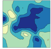
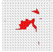
For a continuous spatial domain, the excursion function can be approximated using computed at discrete point locations. The main idea is to interpolate assuming monotonicity of the random field between the discrete computation locations. Specifically, assume that the values of correspond to the values at the vertices of some triangulated mesh such as the one shown in the left panel of Figure 2. If the excursion set should be computed for some specific value of , one has to find the contour for . For interpolation to a location within a specific triangle with corners in and , \pkgexcursions by default uses log-linear interpolation, . Here are the barycentric coordinates of within the triangle.
Further technical details of the continuous domain construction are given in Bolin and Lindgren (2016b). Studies of the resulting continuous domain excursion sets in Bolin and Lindgren (2016b) indicate that the log-linear interpolation method results in sets with coverage probability on target or slightly above target for large target probabilities. An example of a continuous domain excursion set for a triangulated mesh is shown in the middle panel of Figure 2. In the right panel of the figure, the interpolated function is shown. The code that generates the figure is explained in the next section.
3 Implementation
The functions in \pkgexcursions can be divided into four main categories depending on what they compute: (1) Excursion sets and credible regions for contour curves, (2) Quality measures for contour maps, (3) Simultaneous confidence bands, and (4) Utility such as Gaussian integrals and continuous domain mappings. The main functions come in at least three different versions taking different input: (1) The parameters of a Gaussian process, (2) results from an analysis using the \proglangR-\pkgINLA software package, and (3) Monte Carlo simulations of the process. These different categories are described in further detail below.
Much of the computations in the package is done in C functions. These functions use methods from a number of C and Fortran libraries, such as \codeBLAS (Dongarra et al., 1990), \codeLAPACK (Anderson et al., 1999), and \codeCHOLMOD (Chen et al., 2008) for efficient matrix manipulations together with function from the GNU Scientific library (Galassi and Gough, 2006) and several different reordering methods. Notably, the \codeCAMD library (Amestoy et al., 1996, 2004) is used for constrained approximate minimum degree orderings.
As an example that will be used to illustrate the methods in later sections, we generate data at some locations where is a Gaussian random field specified using a stationary SPDE model (Lindgren et al., 2011).
R> x <- seq(from = 0, to = 10, length.out = 20)R> mesh <- inla.mesh.create(lattice = inla.mesh.lattice(x = x, y = x),+ extend = FALSE, refine = FALSE)R> spde <- inla.spde2.matern(mesh, alpha = 2)R> obs.loc <- 10 * cbind(runif(100), runif(100))R> Q <- inla.spde2.precision(spde, theta = c(log(sqrt(0.5)), 0))R> x <- inla.qsample(Q = Q, seed = seed)
Based on the observations, we calculate the posterior distribution of the latent field, which is Gaussian with mean \codemu.post and precision matrix \codeQ.post, these are computed as follows. We refer to Lindgren and Rue (2015) for details about the \proglangR-\pkgINLA related details in the code.
R> A <- inla.spde.make.A(mesh = mesh, loc = obs.loc)R> sigma2.e = 0.01R> Y <- as.vector(A %*% x + rnorm(100) * sqrt(sigma2.e))R> Q.post <- (Q + (t(A) %*% A) / sigma2.e)R> mu.post <- as.vector(solve(Q.post, (t(A) %*% Y) / sigma2.e))
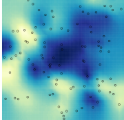

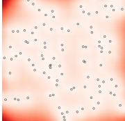

Figure 1 shows the posterior mean and the posterior standard deviations. A contour map of the posterior mean is shown in Figure 2.


3.1 Excursion sets and contour credible regions
The main function for computing excursion sets and contour credible regions is excursions. A typical call to the function looks like
R> res.exc <- excursions(mu = mu.post, Q = Q.post, alpha = 0.1, type = ’>’,+ u = 0, F.limit = 1)
Here, \codemu and \codeQ are the mean vector and precision matrix for the joint distribution of the Gaussian vector \codex. The arguments \codealpha, \codeu, and \codetype are used to specify what type of excursion set that should be computed: \codealpha is the error probability, \codeu is the excursion or contour level, and \codetype determines what type of region that is considered: ’>’ for positive excursion regions, ’<’ for negative excursion regions, ’!=’ for contour avoiding regions, and ’=’ for contour credibility regions. Thus, the call above computes the excursion set .
The argument \codeF.limit is used to specify when to stop the computation of the excursion function. In this case with \codeF.limit=1, all values of are computed, but the computation time can be reduced by decreasing the value of \codeF.limit.
The function has the EB method as default strategy for handling the possible latent Gaussian structure. In the simulated example, the likelihood is Gaussian and the parameters are assumed to be known, so the EB method is exact. The QC method can be used instead by specifying \codemethod=’QC’. In this case, the argument \coderho should be used to also provide a vector with point-wise marginal probabilities: for positive excursions and contour regions, and for negative excursions. In the situation when is Gaussian but is not, the marginal probabilities should be calculated under the distribution and \codemu and \codeQ should be chosen as the mean and precision for the distribution where is the MAP or ML estimate of the parameters.
3.1.1 The INLA interface
The function \codeexcursions.inla is used to compute excursion sets and credible regions for contour curves for latent Gaussian models that have been estimated using \proglangR-\pkgINLA. It takes the same arguments \codeexcursions, except that \codemu and \codeQ are replaced with arguments related to \proglangR-\pkgINLA. A basic call to the function \codeexcursions.inla looks like
R> excursions.inla(result.inla, name, alpha, u, type) Here \coderesult.inla is the output from a call to the \codeinla function, and \codename is the name of the component in the output that the computations should be done for. For more complicated models, one typically specifies the model in \proglangR-\pkgINLA using an \codeinla.stack object. If this is done, the call to \codeexcursions.inla will instead look like
R> excursions.inla(result.inla, stack, tag, alpha, u, type) Here \codestack is now the stack object and \codetag is the name of the component in the stack for which the computations should be done. The typical usage of the \codetag argument is to have one part of the stack that contains the locations where measurements are taken, and another that contains the locations where the output should be computed.
excursions.inla has support for all strategies described in Section 2 for handling latent Gaussian structures: The argument \codemethod can be one of \code’EB’, \code’QC’, \code’NI’, \code’NIQC’, and \code’iNIQC’.
3.1.2 Analysis of Monte Carlo samples
The function excursions.mc can be used to post-process Monte Carlo model simulations in order to compute excursion sets and credible regions. For this function, the model is not specified explicitly. Instead a matrix \codeX containing Monte Carlo simulations of the dimensional process of interest is provided. A basic call to the function looks like
R> excursions.mc(X, u, type) where \codeu again determines the level of interest and \codetype defines the type of set that should be computed. It is important to note that this function does all computations purely based on the Monte Carlo samples that are provided, and it does not use any of the computational methods based on sequential importance sampling for Gaussian integrals that the is the basis for the previous methods. This means that this function in one sense is more general as \codeX can be samples from any model, not necessarily a latent Gaussian model. The price that has to be payed for this generality is that the only way of increasing the accuracy of the results is to increase the number of Monte Carlo samples that are provided to the function.
3.2 Analysis of contour maps
The main function for analysis of contour maps is \codecontourmap. A basic call to the function looks like
R> res.con <- contourmap(mu = mu.post, Q = Q.post, n.levels = 4,+ alpha = 0.1, compute = list(F = TRUE, measures = c("P0")))
Here, \codemu is again the mean value and \codeQ is the precision matrix of the model. The parameter \coden.levels sets the number of contours that should be used in the contour map, and these are spaced equidistant in the range of \codemu by default. Other types of contour maps can be obtained using the \codetype argument. For manual specification of the levels, the \codelevels argument can be used instead. By default, the function computes the specified contour map but no quality measures and it does not compute the contour map function. If quality measures should be computed, this is specified using the \codecompute argument. This argument is also used to decide whether the contour map function should be computed.
As for \codeexcursions, this function comes in two other versions depending on the form of the input: \codecontourmap.inla for model specification using an \proglangR-\pkgINLA object, or \codecontourmap.mc for model specification using Monte Carlo simulations of the model. The model specification using these functions is identical to that in the corresponding \codeexcursions functions.
3.3 Continuous domain interpretations
A common scenario is that the input used in \codecontourmap or \codeexcursions represents the value of the model at some discrete locations in a continuous domain of interest. In this case, the function \codecontinuous can be used to interpolate the discretely computed values by assuming monotonicity of the random field in between the discrete computation locations, as discussed in Section 2. A typical calls to the function looks like
R> sets.exc <- continuous(ex = res.exc, geometry = mesh, alpha = 0.1) Here \codeex is the result of the call to \codecontourmap or \codeexcursions and \codealpha is the error probability of interest for the excursion set or credible region computation. The argument \codegeometry specifies the geometric configuration of the values in input \codeex, either as a general triangulation geometry or as a lattice. A lattice can be specified as an object of the form \codelist(x, y) where \codex and \codey are vectors, or as \codelist(loc, dims) where \codeloc is a two-column matrix of coordinates, and \codedims is the lattice size vector. If \proglangR-\pkgINLA is used, the lattice can also be specified as an \codeinla.mesh.lattice object. In all cases, the input is treated topologically as a lattice with lattice boxes that are assumed convex. A triangulation geometry is specified as an \codeinla.mesh object. Finally, an argument \codeoutput can be used to specify what type of object should be generated. The options are currently \codesp which gives a \codeSpatialPolygons (Bivand et al., 2013) object, and \codeinla which gives an \codeinla.mesh.segment object.
3.4 Simultaneous confidence bands
The function \codesimconf can be used for calculating simultaneous confidence bands for a Gaussian process . A basic call to the function looks like
R> simconf(alpha, mu, Q) where \codealpha is the coverage probability, \codemu is the mean value vector for the process, and \codeQ is the precision matrix for the process. The function has a few optional arguments similar to those of \codeexcursions, all listed in the documentation of the function. The function returns upper and lower limits for both pointwise and simultaneous confidence bands.
As for \codeexcursions and \codecontourmap, there is also a version of \codesimconf that can be used to analyze \proglangR-\pkgINLA models (\codesimconf.inla) and a version that can analyze Monte Carlo samples (\codesimconf.mc). Furthermore, there is a version \codesimconf.mixture which is used to compute simultaneous confidence regions for Gaussian mixture models with a joint distribution on the form
This particular function was used to analyze the models in Bolin et al. (2015) and Guttorp et al. (2014), but is also used internally by \codesimconf.inla.
3.5 Gaussian integrals
Among the utility functions in the package, the function \codegaussint can be especially useful also in a larger context. It contains the implementation of the sequential importance sampling method for computing Gaussian integrals, described in Section 2. This function has two features that separates it from many other functions for computing Gaussian integrals: Firstly it is based on the precision matrix of the Gaussian distribution, and sparsity of this matrix can be utilized to decrease computation time. Secondly, the integration can be stopped as soon as the value of the integral in the sequential integration goes below some given value . If one only is interested in the exact value of the integral given that it is larger than some value , this option can save a lot of computation time.
A basic call to the function looks like
R> gaussint(mu, Q, a, b) where \codemu is the mean value vector, \codeQ is the precision matrix, \codea is a vector of the lower limits in the integral, and \codeb contains the upper integration limits. If the Cholesky factor of \codeQ is known beforehand, this can be supplied to the function using the \codeQ.chol argument. An argument \codealpha is used to set the computational limit for the integral. The function returns an estimate of the integral as well as an error estimate. If the error estimate is too high, the precision can be increased by increasing the \coden.iter argument of the function.
3.6 Plotting
The \pkgexcursions package contains various functions that are useful for visualization. The function \codetricontourmap can be used for visualization of contour maps computed on triangulated meshes. The following code plots the posterior mean using the contour map we previously computed.
R> set.sc <- tricontourmap(mesh, z = mu.post, levels = res.con$u)R> cmap <- colorRampPalette(brewer.pal(9, "YlGnBu"))(100)R> cols <- contourmap.colors(res.con, col = cmap)R> plot(set.sc$map, col = cols) Here \codecontourmap.colors is used to find appropriate colors for each set in the contour map, based on the color map \codecmap that was defined using the \pkgRColorBrewer (Neuwirth, 2014) package. The results of the following commands are shown in Figure 2. The estimated excursion set , can be visualized as
R> plot(sets.exc$M["1"], col = "red", xlim = range(mesh$loc[,1]),+ ylim = range(mesh$loc[,2]))R> plot(mesh, vertex.color = rgb(0.5, 0.5, 0.5), draw.segments = FALSE,+ edge.color = rgb(0.5, 0.5, 0.5), add = TRUE) The second \codeplot command adds the mesh to the plot so that we can see how the set is interpolated by the \codecontinuous function. Finally, the interpolated excursion function , can be plotted easily using the \codeinla.mesh.projector function from the \proglangR-\pkgINLA package.
R> cmap.F <- colorRampPalette(brewer.pal(9, "Greens"))(100)R> proj <- inla.mesh.projector(sets.exc$F.geometry, dims = c(200, 200))R> image(proj$x, proj$y, inla.mesh.project(proj, field = sets.exc$F),+ col = cmap.F, axes = FALSE, xlab = "", ylab = "", asp = 1)R> con <- tricontourmap(mesh, z = mu.post, levels = 0)R> plot(con$map, add = TRUE) The final two lines computes the level zero contour curve and plots it in the same figure as the interpolated excursion function. The colorbars in the figures are plotted using the \pkgfields (Douglas Nychka et al., 2015) package.
4 Two applications
In this section, two examples are used to illustrate how \pkgexcursions can be used.
4.1 Time series data: Tokyo rainfall
To illustrate the methods in the package, we use the much analyzed binomial time series from Kitagawa (1987). Each day during the years 1983 and 1984, it was recorded whether there was more than 1 mm rainfall in Tokyo. Of interest is to study the underlying probability of rainfall as a function of day of the year. The data is modelled as for calendar day . Here for all days except for February 29 () which only occurred during the leap year of 1984. The probability is modeled as a logit-transformed Gaussian process.
The model and the following \proglangR-\pkgINLA implementation of the model is described further in Lindgren and Rue (2015).
R> data("Tokyo")R> mesh <- inla.mesh.1d(seq(1, 367, length = 25), interval = c(1, 367),+ degree = 2, boundary = "cyclic")R> kappa <- 1e-3R> tau <- 1 / (4 * kappa^3)^0.5R> spde <- inla.spde2.matern(mesh, constr = FALSE, theta.prior.prec = 1e-4,+ B.tau = cbind(log(tau), 1), B.kappa = cbind(log(kappa), 0))R> A <- inla.spde.make.A(mesh, loc = Tokyo$time)R> time.index <- inla.spde.make.index("time", n.spde = spde$n.spde)R> stack <- inla.stack(data = list(y = Tokyo$y, link = 1, Ntrials = Tokyo$n),+ A = list(A), effects = list(time.index), tag = "est")R> formula <- y ~ -1 + f(time, model = spde)R> data <- inla.stack.data(stack)
Next, the model is estimated using the \codeinla function. Since we want to analyze the output using \pkgexcursions, the additional option \codecontrol.compute = list(config = TRUE) must be specified in the \codeinla function. This makes the function save some extra output needed by \pkgexcursions.
R> result <- inla(formula, family = "binomial", data = data,+ Ntrials = data$Ntrials, control.predictor = list(+ A = inla.stack.A(stack), link = data$link, compute = TRUE),+ control.compute = list(config = TRUE))
We now have estimates of the posterior mean and marginal confidence intervals for the probability of rain for each day. However, if we also want joint confidence bands, we can estimate these using \codesimconf.inla as
R> res <- simconf.inla(result, stack, tag = "est", alpha = 0.05, link = TRUE)
Note the argument \codelink=TRUE which tells the function that the results should be returned in the scale of the data, and not in the scale of the linear predictor. Next, we plot the results, showing the marginal confidence bands with dashed lines and the simultaneous confidence band with dotted lines. The results are shown in Figure 3.
R> index <- inla.stack.index(stack, "est")$dataR> plot(Tokyo$time, Tokyo$y / Tokyo$n, xlab = "Day", ylab = "Probability")R> lines(result$summary.fitted.values$mean[index])R> matplot(cBind(res$a.marginal, res$b.marginal), type = "l", lty = 2,+ col = 1, add = TRUE)R> matplot(cBind(res$a, res$b), type = "l", lty = 3, col = 1, add = TRUE)

4.2 Spatial data: Parana precipitation
We will now use a spatial dataset to illustrate how \pkgexcursions can be used. In order to keep the parts of the code that are not relevant to \pkgexcursions brief, we again use data available in \proglangR-\pkgINLA. The dataset consists of daily rainfall data for each day of the year 2011, at 616 locations in and around the stated of Paraná in Brazil. In the following analysis, we analyse the data from the month of January.
The statistical model used for the data is a latent Gaussian model, where the precipitation measurements are assumed to be -distributed with a spatially varying mean. The mean is modeled as a log-Gaussian Matérn field specified as an SPDE model. Details of the current model model and the following INLA implementation can be found in the SPDE tutorial available on the \proglangR-\pkgINLA homepage, see Wallin and Bolin (2015) for an analysis of the data using a different non-Gaussian SPDE model.
We start by loading the data and defining the model:
R> data("PRprec")R> data("PRborder")R> Y <- rowMeans(PRprec[, 3 + (1 : 31)])R> ind <- !is.na(Y)R> Y <- Y[ind]R> coords <- as.matrix(PRprec[ind, 1 : 2])R> b <- inla.nonconvex.hull(coords, -0.03, -0.05, resolution = c(100, 100))R> prmesh <- inla.mesh.2d(boundary = b, max.edge = c(.45, 1), cutoff = 0.2)R> A <- inla.spde.make.A(prmesh, loc = coords)R> spde <- inla.spde2.matern(prmesh, alpha = 2)R> mesh.index <- inla.spde.make.index(name = "field", n.spde = spde$n.spde)
The measurement stations are spatially irregular, but we are interested in making predictions to a regular lattice within the state. In order to do continuous domain interpretations, we define the lattice locations as a lattice object using the \codesubmesh function of the \codeexcursions package. The function \codeinout from the package \pkgsplancs (Rowlingson and Diggle, 2015) is used to find the locations on the lattice that are within the region of interest.
R> nxy <- c(50, 50)R> projgrid <- inla.mesh.projector(prmesh, xlim = range(PRborder[, 1]),+ ylim = range(PRborder[, 2]), dims = nxy)R> xy.in <- inout(projgrid$lattice$loc, cbind(PRborder[, 1], PRborder[, 2]))R> submesh = submesh.grid(matrix(xy.in, nxy[1], nxy[2]),+ list(loc=projgrid$lattice$loc, dims = nxy))
We now define the \codestack objects and estimate the model using \codeinla. Again note that we have to set the \codecontrol.compute argument of the results is to be used by \pkgexcursions.
R> A.prd <- inla.spde.make.A(prmesh, loc = submesh$loc)R> stk.prd <- inla.stack(data=list(y = NA), A = list(A.prd, 1),+ effects=list(c(mesh.index, list(Intercept = 1)),+ list(lat = submesh$loc[,2], lon = submesh$loc[,1])), tag = "prd")R> stk.dat <- inla.stack(data = list(y = Y), A=list(A, 1),+ effects = list(c(mesh.index, list(Intercept = 1)),+ list(lat = coords[,2], lon = coords[,1])), tag = "est")R> stk <- inla.stack(stk.dat, stk.prd)R> r <- inla(y ~ -1 + Intercept + f(field, model = spde), family = "Gamma",+ data = inla.stack.data(stk), control.compute = list(config = TRUE),+ control.predictor = list(A = inla.stack.A(stk), compute = TRUE, link=1))
We now want to find areas that likely experienced large amounts of precipitation. In the following code, we compute the excursion set for the posterior mean for the level mm of precipitation. To indicate that this level is in the scale of the data, and not in the scale of the linear predictor, we use the \codeu.link=TRUE argument in the \codeexcursions call.
R> exc = excursions.inla(r, stk, tag = "prd", u = 7, u.link = TRUE,+ type = ">", F.lim = 0.6, method = ’QC’)R> sets <- continuous(exc, submesh, alpha = 0.1) We also compute the contour curve for the level of interest on the continuous domain, using the \codetricontourmap function.
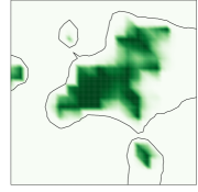
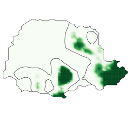
R> con <- tricontourmap(submesh, z=exc$mean, levels = log(7)) We plot the resulting continuous domain excursion function together with the contour curve using the following commands. The result is shown in the right panel of Figure 4.
R> proj <- inla.mesh.projector(sets$F.geometry, dims = c(300,200))R> image(proj$x, proj$y, inla.mesh.project(proj, field = sets$F),+ col = cmap.F, axes = FALSE, xlab = "", ylab = "", asp = 1)R> plot(con$map, add = TRUE)
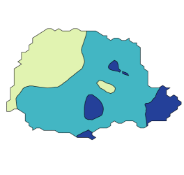


To visualize the posterior mean using a contour map using the following commands
R> lp <- contourmap.inla(r, stack = stk, tag = "prd", n.levels = 2,+ compute = list(F = FALSE))R> tmap <- tricontourmap(submesh, z = exc$mean, levels = lp$meta$levels)R> plot(tmap$map, col = contourmap.colors(lp, col = cmap)) Here, the \codecontourmap.inla computes the levels of the contour map and \codetricontourmap computes the contour map on the mesh. Finally, \codecontourmap.colors is used to compute appropriate colours for visualising the contour map. The result is shown in the left panel of Figure 4.
The contour map we computed had two contours, and a relevant question is now if this is an appropriate number. To investigate this, we compute the quality measure for this contour map and for contour maps with one and three levels.
R> lp1 <- contourmap.inla(r, stack = stk, tag = "prd", n.levels = 1,+ compute = list(F = FALSE, measures = c("P2")))R> lp2 <- contourmap.inla(r, stack = stk, tag = "prd", n.levels = 2,+ compute = list(F = FALSE, measures = c("P2")))R> lp3 <- contourmap.inla(r, stack = stk, tag = "prd", n.levels = 3,+ compute = list(F = FALSE, measures = c("P2")))R> cat(c(lp1$P2, lp2$P2, lp3$P2))
1 0.4785692 0.004764646 We see that using only one contour gives very high credibility, whereas using three contours give a credibility that is close to zero. The contour map with two contours has a credibility around and seems to be a good choice for this application.
5 Discussion
The \pkgexcursions package was first developed for calculating probabilistic excursion sets and contour credible regions for latent Gaussian stochastic processes and fields. Since the early versions, the scope of the package has grown and it now contains functions for several other related computations, such as simultaneous confidence bands, uncertainty quantification of contour maps, and computations of Gaussian integrals.
Some of the functionaliy in \pkgexcursions can also be found in other packages. For example, \pkgExceedanceTools (French, 2014) provides an alternative method for computing excursion sets and uncertainty regions for contour curves for Gaussian models. The package \pkgmvtnorm (Genz et al., 2016) contains functions for computing integrals of Gaussian distributions, but does not have support for computations based on sparse precision matrices. Finally, there are numerous packages with the ability to compute simultaneous confidence bands for various models, such as semiparametric regression models using \pkgAdaptFitOS (Wiesenfarth et al., 2012) or nonparametric regression models for functional data using \pkgSCBmeanfd (Degras, 2016). Comparing the methods in \pkgexcursions to the corresponding methods in these packages is an intersting topic for future studies.
Future work also includes further development of the package, and new features are added as they are needed. One main focus for the current development is to add functionality for large scale computations, where sparse Cholesky factorisation is computationally infeasible. We also plan to add functionality for computations needed in spatial extreme value theory, where certain Gaussian integrals often are needed during likelihood inference. Finally, the technical aspects of the functions are also being improved, and future releases will introduce improvements to both the continuous domain interpretations and to the algorithms for finding the largest excursion sets.
References
- Amestoy et al. (1996) Amestoy P, Davis TA, Duff IS (1996). “An Approximate Minimum Degree Ordering Algorithm.” SIAM Journal on Matrix Analysis and Applications, 17(4), 886–905.
- Amestoy et al. (2004) Amestoy P, Davis TA, Duff IS (2004). “Algorithm 837: AMD, an Approximate Minimum Degree Ordering Algorithm.” ACM Transactions on Mathematical Software, 30(3), 381–388.
- Anderson et al. (1999) Anderson E, Bai Z, Bischof C, Blackford L, Demmel J, Dongarra J, Du Croz J, Hammarling S, Greenbaum A, McKenney A, , Sorensen D (1999). LAPACK Users’ Guide (Third Ed.). Society for Industrial and Applied Mathematics, Philadelphia, PA, USA.
- Beaky et al. (1992) Beaky MM, Scherrer RJ, Villumsen JV (1992). “Topology of Large-Scale Structure in Seeded Hot Dark Matter Models.” Astrophysical Journal, Part 1, 387, 443–448.
- Bivand et al. (2013) Bivand RS, Pebesma E, Gómez-Rubio V (2013). Applied Spatial Data Analysis with \proglangR. Springer New York.
- Bolin et al. (2015) Bolin D, Guttorp P, Januzzi A, Jones D, Novak M, Podschwit H, Richardson L, Särkkä A, Sowder C, Zimmerman A (2015). “Statistical Prediction of Global Sea Level From Global Temperature.” Statistica Sinica, 25, 351–367.
- Bolin and Lindgren (2015) Bolin D, Lindgren F (2015). “Excursion and Contour Uncertainty Regions for Latent Gaussian Models.” Journal of the Royal Statistical Society B, 77, 85–106.
- Bolin and Lindgren (2016a) Bolin D, Lindgren F (2016a). \pkgexcursions: Excursion Sets and Contour Credible Regions for Latent Gaussian Models. \proglangR package version 2.2.2, URL https://CRAN.R-project.org/package=excursions.
- Bolin and Lindgren (2016b) Bolin D, Lindgren F (2016b). “Quantifying the Uncertainty of Contour Maps.” Journal of Computational and Graphical Statistics (in press).
- Bolin et al. (2009) Bolin D, Lindström J, Eklundh L, Lindgren F (2009). “Fast Estimation of Spatially Dependent Temporal Vegetation Trends Using Gaussian Markov Random Fields.” Computational Statistics and Data Analysis, 53, 2885–2896.
- Cameletti et al. (2013) Cameletti M, Lindgren F, Simpson D, Rue H (2013). “Spatio-Temporal Modeling of Particulate Matter Concentration Through the SPDE Approach.” AStA Advances in Statistical Analysis, 97(2), 109–131.
- Chen et al. (2008) Chen Y, Davis TA, Hager WW, Rajamanickam S (2008). “Algorithm 887: CHOLMOD, Supernodal Sparse Cholesky Factorization and Update/Downdate.” ACM Transactions on Mathematical Software (TOMS), 35(3), 22.
- Degras (2016) Degras D (2016). \pkgSCBmeanfd: Simultaneous Confidence Bands for the Mean of Functional Data. \proglangR package version 1.2.2, URL https://CRAN.R-project.org/package=SCBmeanfd.
- Dongarra et al. (1990) Dongarra JJ, Du Croz J, Hammarling S, Duff IS (1990). “A Set of Level 3 Basic Linear Algebra Subprograms.” ACM Transactions on Mathematical Software (TOMS), 16(1), 1–17.
- Douglas Nychka et al. (2015) Douglas Nychka, Reinhard Furrer, John Paige, Stephan Sain (2015). “\pkgfields: Tools for Spatial Data.” 10.5065/D6W957CT. \proglangR package version 8.4-1, URL www.image.ucar.edu/fields.
- Eklundh and Olsson (2003) Eklundh L, Olsson L (2003). “Vegetation Index Trends for the African Sahel 1982–1999.” Geophysical Research Letters, 30, 1430–1433.
- French (2014) French J (2014). \pkgExceedanceTools: Confidence Regions for Exceedance Sets and Contour Lines. \proglangR package version 1.2.2, URL https://CRAN.R-project.org/package=ExceedanceTools.
- Furrer et al. (2007) Furrer R, Knutti R, Sain SR, Nychka D, A MG (2007). “Spatial Patterns of Probabilistic Temperature Change Projections From a Multivariate Bayesian Analysis.” Geophysical Research Letters, 34.
- Galassi and Gough (2006) Galassi M, Gough B (2006). “GNU Scientific Library: Reference Manual.”
- Genz et al. (2016) Genz A, Bretz F, Miwa T, Mi X, Leisch F, Scheipl F, Hothorn T (2016). \pkgmvtnorm: Multivariate Normal and t Distributions. \proglangR package version 1.0-5, URL http://CRAN.R-project.org/package=mvtnorm.
- Guttorp et al. (2014) Guttorp P, Januzzi A, Novak M, Podschwit H, Richardson L, Sowder CD, Zimmerman A, Bolin D, Särkkä A (2014). “Assessing the Uncertainty in Projecting Local Mean Sea Level From Global Temperature.” Journal of Applied Meteorology and Climatology, 53(9), 2163–2170.
- Kitagawa (1987) Kitagawa G (1987). “Non-Gaussian State-Space Modeling of Nonstationary Time Series.” Journal of the American statistical association, 82(400), 1032–1041.
- Lindgren and Rue (2015) Lindgren F, Rue H (2015). “Bayesian Spatial and Spatiotemporal Modelling With \pkgR-INLA.” Journal of Statistical Software, 63(19).
- Lindgren et al. (2011) Lindgren F, Rue H, Lindström J (2011). “An Explicit Link Between Gaussian Fields and Gaussian Markov Random Fields: The Stochastic Partial Differential Equation Approach (With Discussion).” Journal of the Royal Statistical Society B, 73, 423–498.
- Marchini and Presanis (2003) Marchini J, Presanis A (2003). “Comparing Methods of Analyzing fMRI Statistical Parametric Maps.” NeuroImage, 22, 1203–1213.
- Neuwirth (2014) Neuwirth E (2014). \pkgRColorBrewer: ColorBrewer Palettes. \proglangR package version 1.1-2, URL https://CRAN.R-project.org/package=RColorBrewer.
- \proglangR Core Team (2013) \proglangR Core Team (2013). \proglangR: A Language and Environment for Statistical Computing. R Foundation for Statistical Computing, Vienna, Austria. URL http://www.R-project.org/.
- Rowlingson and Diggle (2015) Rowlingson B, Diggle P (2015). \pkgsplancs: Spatial and Space-Time Point Pattern Analysis. \proglangR package version 2.01-37, URL https://CRAN.R-project.org/package=splancs.
- Rue et al. (2009) Rue H, Martino S, Chopin N (2009). “Approximate Bayesian Inference for Latent Gaussian Models Using Integrated Nested Laplace Approximations (With Discussion).” Journal of the Royal Statistical Society B, 71(2), 319–392.
- Sain et al. (2011) Sain SR, Furrer R, Cressie N (2011). “A Spatial Analysis of Multivariate Output From Regional Climate Models.” The Annals of Applied Statistics, 5, 150–175.
- Wallin and Bolin (2015) Wallin J, Bolin D (2015). “Geostatistical Modelling Using Non-Gaussian Matérn Fields.” Scandinavian Journal of Statistics, pp. 872–890.
- Wiesenfarth et al. (2012) Wiesenfarth M, Krivobokova T, Klasen S, Sperlich S (2012). “Direct Simultaneous Inference in Additive Models and its Application to Model Undernutrition.” Journal of the American Statistical Association, 107(500), 1286–1296.