A globally convergent numerical method for a 3D coefficient inverse problem with a single measurement of multi-frequency data
Abstract
The goal of this paper is to reconstruct spatially distributed dielectric constants from complex-valued scattered wave field by solving a 3D coefficient inverse problem for the Helmholtz equation at multi-frequencies. The data are generated by only a single direction of the incident plane wave. To solve this inverse problem, a globally convergent algorithm is analytically developed. We prove that this algorithm provides a good approximation for the exact coefficient without any a priori knowledge of any point in a small neighborhood of that coefficient. This is the main advantage of our method, compared with classical approaches using optimization schemes. Numerical results are presented for both computationally simulated data and experimental data. Potential applications of this problem are in detection and identification of explosive-like targets.
Keywords. global convergence, coefficient inverse problem, inverse medium problem, coefficient identification, multi-frequency data, experimental data, single measurement
AMS subject classification. 35R30, 78A46, 65C20
1 Introduction
We are interested in this paper in the inverse problem of recovering the spatially distributed dielectric constant of the Helmholtz equation from a single boundary measurement of its solution. This inverse problem is also called a coefficient inverse problem with a single measurement data (CIP). CIPs are both ill-posed and highly nonlinear. Therefore, an important and challenging question to address in a numerical treatment of a CIP is: How to obtain at least one point in a sufficiently small neighborhood of the exact coefficient without any advanced knowledge of this neighborhood? As soon as this point is obtained, one can refine it using one of well established techniques, such as, e.g., a Newton-like method or a gradient-like method, see, e.g., [4]. It is well known that a rigorous guarantee of convergence of such a technique to the exact solution can be obtained only if the starting point of iterations belongs to a sufficiently small neighborhood of that solution.
We call a numerical method for a CIP approximately globally convergent (globally convergent in short, or GCM) if: (1) a theorem is proved, which claims that, under a reasonable mathematical assumption, this method delivers at least one point in a sufficiently small neighborhood of the exact solution without any advanced knowledge of this neighborhood, (2) the error of the approximation of the true solution depends only on the level of noise in the boundary data and on some discretization errors. Such an assumption is necessary due to the well known tremendous challenge of the goal to develop those numerical methods for CIPs, which positively address the question posed in the previous paragraph. This is especially true for CIPs with single measurement data, which are known to be one of the most challenging ones. In our particular case that assumption amounts dropping a small term of an asymptotic expansion, and this is used only on the zero iteration of our method, see Section 4.3. Due to our target application, the CIP considered here is a CIP with single measurement data. We refer to [5, 6] for detailed discussions of the notion of the approximate global convergence.
Our CIP has many applications in sonar imaging, geographical exploration, medical imaging, near-field optical microscopy, nano-optics, see, e.g., [13]. However, the target application of this paper is in imaging of dielectric constants of antipersonnel mines and improvised explosive devices (IEDs). We model the so-called “stand off” detection, which means that we use only backscatter data. Currently the radar community relies only on the intensity of radar images [37] to see the geometrical information such as, e.g., sizes and shapes of targets. Thus, we hope that the additional information about values of dielectric constants of targets, which our method delivers, might lead in the future to a better differentiation between explosives and clutter.
CIPs of wave propagation are a part of a bigger subfield, Inverse Scattering Problems (ISPs). ISPs attract a significant attention of the scientific community. There is a large body of the literature on imaging methods for reconstructing geometrical information about targets, such as their shapes, sizes and locations. We refer to, e.g., [2, 3, 9, 12, 19, 21, 30, 31] and references therein for well-known imaging techniques in inverse scattering such as level set methods, sampling methods, expansion methods, and shape optimization methods.
The most popular approach to solve CIPs is nonlinear optimization methods minimizing some cost functionals, see, e.g., [4, 10, 15, 17, 40]. However, in general, such functionals are non-convex and might have multiple local minima and ravines, see, e.g., Figure 1 in [36] for a convincing example of the latter. Therefore, a good initial guess for the true solution is required. Such a first guess might be found by solving the linearized problem using the Born approximation. As a results, the relative target/background contrast is assumed to be small, while it is actually high in many real world applications (see, e.g. the table of dielectric constants on the web site of Honeywell with shortened link by Google https://goo.gl/kAxtzB). This is one of the reasons for us to establish a GCM to solve this inverse problem without knowing a good initial approximation of the true solution.
In [5, 6] an approximately globally convergent method was established for a CIP with single measurement data for a wave-like PDE using Laplace transform. That method was verified on experimental data, see [23, 27, 38, 39], and references cited therein. The GCM of [5, 6] was extended in [11] to a CIP for a different wave equation.
The goal of this paper is to develop a new GCM for a CIP for the Helmholtz equation in with a single measurement of multi-frequency data. In other words, we now work in the frequency domain. Formally, the Helmholtz equation can be obtained via the Fourier transform with respect to time of the solution of the hyperbolic equation considered in [5, 6]. One of the reasons for us not to do so is because the kernel of the Laplace transform, used in the previous GCM [5, 6], decays exponentially fast and therefore some significant information might be lost. The main difficulty in developing this new GCM is to work with complex-valued functions where the maximum principle, which plays an important role in the previous GCM, is no longer applicable. We first develop the theory for the method. Next, we conduct a numerical study for computationally simulated data. At the end, we present one numerical example for experimental data. In fact, this is one of results of the work [32] of our group.
In [32] the method of the current publication was successfully tested on experimental data collected in the frequency domain. In addition, in [26] this method was tested on experimental data collected in the time domain: after a certain preprocessing procedure, these data were “moved” in the frequency domain via the Fourier transform. In both works [26, 32], results of the reconstructions of locations and dielectric constants of inclusions were quite accurate. The 1D version of the method under consideration along with its performance for experimental data can be found in [24].
As to the CIPs with multiple measurement, i.e., the Dirichlet-to-Neumann map data, we mention the recent works [1, 20, 33] and references cited therein, where reconstruction procedures are developed, which do not require a priori knowledge of a small neighborhood of the exact coefficient.
The paper is organized as follows. In Section 2, we state the forward and inverse problems. In Section 3, we discuss some facts about the Lippmann-Schwinger equation. We need these facts for the analysis of our numerical method. In Section 4, we establish an integral differential equation for the CIP and derive an initial approximation for the target coefficient. In Section 5, we present our globally convergent numerical method and formulate the corresponding algorithm. In Section 6, we prove the main theorem of this paper: the global convergence theorem. In addition, we discuss this theorem in Section 6 and present the main discrepancies between the theory and computations. In Section 7, we present our numerical results for both computationally simulated and experimental data. Section 8 is devoted to a short summary.
2 Problem statement
2.1 Assumptions on the coefficient
Below Let be the ball of the radius with the center at Let be convex bounded domains and . Here and below are Hölder spaces where is an integer and Let be a function defined in . Throughout the paper we assume that
| (2.1) | ||||
| (2.2) |
The Riemannian metric generated by the function is
| (2.3) |
This metric generates geodesic lines. Let be an arbitrary number. Consider the plane Note that since outside of the domain then geodesic lines are straight lines outside of In particular, since our incident plane wave propagates along the positive direction of the axis (see this section below), we consider for only those parts of geodesic lines which are parallel to the axis. Then these lines intersect the plane orthogonally. Throughout the paper we use the following assumption about the regularity of and geodesic lines generated by the function
Assumption 2.1.
Assume that . Furthermore, for any point there exists unique geodesic line connecting and the plane and such that intersects the plane orthogonally.
The length of the geodesic line is
| (2.4) |
A sufficient condition for the validity of Assumption was found in [35],
Remark 2.1.
-
1.
The conditions in assumption 2.1 are technical ones. We use them only to derive the asymptotic expansion of the function with respect to in Section 4.1. This expansion was proved in [25], where these conditions were used quite essentially. However, they are not imposed in computations, see also Section 6.2.
-
2.
In the case of propagation of electromagnetic waves, as in the experimental data of [26, 32], is the spatially distributed dielectric constant. We assume its independence on the wavenumber since we end up working on a small interval. In this paper, we assume that the total field satisfies the Helmholtz equation rather than the full Maxwell’s system. This is reasonable when the dielectric constant varies so slowly that it is almost constant over the distances of the order of the wavelength, see [7, Chapter 13] for more details. The good accuracy of our results for experimental data of [26, 32] as well as in Section 7.8 of this paper points towards the validity of this assumption.
2.2 The Coefficient Inverse Problem
Below is the wavenumber. Consider the function , which represents the incident plane wave propagating along the positive direction of the axis. Let be the solution of the following problem:
| (2.5) |
The functions and are called the total field, incident field and scattered field respectively.
It is well-known (see [13, Theorem 8.7]) that problem (2.5) has unique solution In fact, for any , see [16, Theorem 6.17]. In this paper, we consider the following problem:
Coefficient Inverse Problem (CIP). Let and be two positive numbers and . Assume that the function
| (2.6) |
is known where is the solution of the problem (2.5). Determine the function for
In the current paper, we develop the theory of our numerical method for this CIP. We also numerically test our method for a CIP with partial data. Since we have only a single direction of the propagation of the incident plane wave, our CIP is an inverse problem with the data from a single measurement event. In this paper, we focus only on the numerical method for our CIP. As to the question of the uniqueness of the solution, it is worth mentioning that currently uniqueness for the single measurement case can be proved only if the homogeneous equation in (2.5) would be replaced with a non-homogeneous one, in which the right hand side would be nonzero everywhere in . The proof of this fact was first introduced in [8] by using the Carleman estimate. There were many works of many authors since then exploring the method of [8]. We refer the reader to review papers [22, 43]. In the case when the right hand side of equation in (2.5) has some zeros, an attempt to address the uniqueness question faces fundamental challenges which are yet unclear how to tackle. Hence, we assume below uniqueness for our CIP.
It is well known in the theory of Ill-Posed Problems that one should assume the existence of the exact solution, which corresponds to the ideal, noiseless data [4, 5, 40]. Hence, throughout the paper, is that exact coefficient and we use the superscript ∗ to indicate functions related to Naturally, we assume that assumption 2.1 is valid for the function
3 Using the Lippmann-Schwinger equation
In this section we use the Lippmann-Schwinger equation to derive some important facts, which we need both for our algorithm and for the convergence analysis. We use here results of Chapter 8 of the book [13]. Denote
In this section the function and it also satisfies conditions (2.1), (2.2). The Lippmann-Schwinger equation for the function is
| (3.1) |
If the function satisfies equation (3.1) for then we can extend it for via substitution these points in the right hand side of (3.1). Hence, to solve (3.1), it is sufficient to find the function only for points Consider the linear operator defined as
| (3.2) |
It follows from Theorem 8.1 of [13] that
| (3.3) |
Here and below denotes different constants which depend only on listed parameters. Therefore, the operator maps to as a compact operator. Hence, the Fredholm theory is applicable to equation (3.1). Lemmata 3.1 and 3.2 follow from Theorem 8.3 and Theorem 8.7 of [13] respectively.
Lemma 3.1.
Lemma 3.2.
Proof.
Lemma 3.3.
For all the solution of the problem (2.5) is infinitely many times differentiable with respect to . Furthermore, and
Let the function be such that
| (3.8) |
The existence of such functions is well known from the Real Analysis course. While Lemmata 3.1 and 3.2 are formulated for the case when the function is real valued, we now consider the case of a complex valued analog of this function. We will need this for our algorithm. Consider a complex valued function . Let . Then
| (3.9) |
We have the lemma.
Lemma 3.4.
Let . Let be the solution of the problem (2.5) in which is replaced with . Consider equation (3.1) in which is replaced with
| (3.10) |
Then there exists a sufficiently small number depending only on listed parameters such that if and , then equation (3.10) has unique solution . Furthermore, the function and
| (3.11) |
where the constant depends only on the listed parameters.
Proof.
Below denotes different positive constants depending on the above parameters. We have . Since, by (2.2), the function outside of the domain , then (3.8) implies that Hence, and . Using notation (3.2), we rewrite equation (3.10) in the following equivalent form
| (3.12) |
where the linear operator is given by
| (3.13) |
We have for any function
| (3.14) |
Therefore,
| (3.15) |
It follows from Lemma 3.2 and the Fredholm theory that the operator has a bounded inverse operator and
| (3.16) |
Hence, using (3.12), we obtain
| (3.17) |
It follows from (3.15) and (3.16) that there exists a sufficiently small number depending on , such that if and then the operator is a contraction mapping. This implies uniqueness and existence of the solution of equation (3.17), which is equivalent to equation (3.10). Also,
| (3.18) |
with a different constant . Furthermore, by (3.3) the function
We now prove estimate (3.11). Let . Since we obtain the following analog of (3.12)
| (3.19) |
Hence, . Hence, (3.15) and (3.18) lead to
| (3.20) |
Next, we rewrite (3.19) as
| (3.21) |
By (3.3) and (3.13) the right hand side of equation (3.21) belongs to the space Hence, using (3.3), (3.14), (3.18) and (3.20), we obtain from (3.21) that
4 Integral differential equation formulation
In this section, we eliminate the target coefficient from the governing equation (2.5). This process leads to an integral differential equation. Solving this equation is equivalent to solving our CIP. Note that this approach is different from locally convergent methods with iterative optimization processes which typically rely on least-squares formulation. Furthermore, under some mathematical assumptions, we rigorously derive a good initial approximation for The analysis relies on the high frequency asymptotic behavior of the total wave in the next section.
4.1 The asymptotics with respect to
Let be the function defined in (2.4). It was proven in [25, Theorem 1 and its consequence (4.26)] that for the asymptotic expansion of the function with respect to is
| (4.1) | |||
| (4.2) |
where the function is defined in and the number depends only on listed parameters. By (4.1) and (4.2), given a coefficient , one can choose a number such that
We note that by (4.1), (4.2) we need only an estimate from the below for the number rather than its exact value. The development of the theory of this paper would become much more complicated if we would work with the numbers which would depend on the function . Hence, from now on, we assume that these numbers are the same for all functions which we consider here. This assumption is supported from the Physics standpoint by our study of experimental data [26, 32]. Thus, below numbers are the same for all functions considered here and also
| (4.3) | |||
| (4.4) |
4.2 The tail function and some auxiliary functions
We obtain from (4.3), (4.4) and a straightforward calculation that the vector , , is free. Hence, there exists a function such that
| (4.5) |
This implies
Therefore,
Hence,
where is a constant. The smoothness of the function and (4.5) imply that . Choosing , we have found a function such that
| (4.6) |
Remark 4.1.
-
1.
The function , , is determined uniquely up to the addition of a constant , . We can choose . This choice determines the function uniquely. We name it the tail function.
-
2.
The choice of does not effect the results of our reconstruction method since we only use the derivatives of (see Algorithm 5.1) instead of
Define the function
| (4.7) |
Lemma 4.1.
For all , the function belongs to . Moreover
| (4.8) | |||
| (4.9) |
for all .
Proof.
The fact that follows immediately from (4.3), (4.4), (4.7) and Lemma 3.3. Now, we prove only (4.8) and (4.9). Differentiating (4.7) with respect to and then multiplying both sides of the resulting equation by , we obtain
Hence, where is independent on . In particular, letting and using (4.6), we have . This implies (4.8).
We next eliminate the function from equation (4.9). To this end, define the function
| (4.10) |
Differentiating equation (4.9) with respect to , we obtain
| (4.11) |
Plugging the function of (4.7) into (4.11), we obtain Lemma 4.13. Keeping in mind our numerical method, it is convenient to consider in this lemma that rather than the above
Lemma 4.2 (integral differential equation).
The function satisfies the following nonlinear integral differential equation
| (4.12) |
for all and Denoting , we have the following boundary condition
| (4.13) |
Now, solving our CIP is equivalent to solving problem (4.11)–(4.13). To do so, we iteratively approximate both functions and using the predictor-corrector scheme. Here approximations for are used as predictors and approximations for are used as correctors. We first start from an approximation for the tail function .
4.3 The initial approximation of the tail function
In this section we introduce a reasonable mathematical assumption mentioned in Section 1. The idea is to find an initial approximation for using the asymptotic behavior of as . Let and let condition (4.3) be fulfilled. We set in (4.1) and then ignore the term for It follows from (4.2) that we can do this uniformly for all Hence, we obtain the following approximate formula
| (4.14) |
Define the function for as in (4.7). Then, the result in Lemma 4.1 is still valid for Since by (4.8) we set, using (4.14),
| (4.15) |
Since is sufficiently large, we can drop the term in (4.15) and obtain
| (4.16) |
Next, since by (4.7) then (4.16) implies that
| (4.17) |
Next, since we obtain from (4.16)
| (4.18) |
Substituting functions from (4.17) and from (4.18) in problem (4.12)–(4.13) at , we obtain via a straightforward calculation
| (4.19) |
Thus, we have obtained the Dirichlet boundary value problem (4.19) for the Laplace equation with respect to the function . Recall that and that the function By the Schauder Theorem [28], there exists unique solution of the problem (4.19).
In practice, however, we have the non-exact boundary data rather than the exact data Thus, we set the first approximation for the tail function as
| (4.20) |
where the function is the solution of the following analog of problem (4.19)
| (4.21) |
Using (4.9), we define the first approximation for the exact coefficient as
| (4.22) |
Lemma 4.3.
Proof.
Remark 4.2.
-
1.
Formulas (4.14)–(4.18) form the first part of our reasonable mathematical assumption mentioned in Section 1. The second part is that we assume that numbers are the same for all functions we consider here, see (4.3), (4.4) and the paragraph above them. We point out that formulas (4.14)–(4.18) are used only on the first iteration of our method. However, we do not use them on follow up iterations.
-
2.
It follows from estimate (4.24) that the first approximation of the exact coefficient belongs to a small neighborhood of , provided that the error in the data is sufficiently small. Therefore, the global convergence property is achieved just at the start of our iterative process.
- 3.
5 The algorithm
We first consider the discretization of problem (4.12)–(4.13) with respect to the wavenumber . Then, we prove the well-posedness of the resulting problem. In the last part of this section, we propose the globally convergent numerical algorithm.
5.1 The discretization of the interval of wavenumbers
To find and from problem (4.12)–(4.13) using an iterative process, we consider a discretization of this problem with respect to the wavenumber . We divide the interval into subintervals with the uniform step size as follows
| (5.1) |
We approximate the function as a piecewise constant function with respect to ,
| (5.2) |
Now, we define
| (5.3) |
Then
Equation (4.12) becomes
| (5.4) |
We use here instead of since we will update the tail function in our algorithm. By Lemma 3.3 So, assuming that the discretization step size is sufficiently small, we replace in (5.4) with . Using again the fact that is sufficiently small, we also drop in (5.4) the nonlinear term as well as the terms However, we do not drop terms since is a sum of other terms, see (5.3). These approximations enable us to simplify the analysis as well as the computations of our method. Using (5.4), we obtain
| (5.5) |
Let Then (4.13) and (5.2) lead to the following Dirichlet boundary condition for the function
| (5.6) |
5.2 The well-posedness of problem (5.5)–(5.6)
In this section we study the existence and uniqueness of the solution of the Dirichlet boundary value problem (5.5)–(5.6). In the case of real-valued functions, existence and uniqueness of the solution follow from [16, Theorem 6.14]. The proof is based on the maximum principle and Schauder Theorem [16, 28]. However, complex-valued functions cause some additional difficulties, since the maximum principle does not work in this case. Still, we can get our desired results for the case of complex-valued functions using the assumption that the norm is sufficiently small. Keeping in mind the convergence analysis in the next section, it is convenient to consider here problem (5.5)–(5.6) in a more general form
| (5.7) |
Lemma 5.1.
Proof.
Below in this paper denotes different positive constants depending only on the domain Let the complex-valued function Consider the following Dirichlet boundary value problem with respect to the function :
| (5.9) |
The Schauder Theorem implies that there exists unique solution of the problem (5.9) and
| (5.10) |
Hence, for each fixed pair , we can define a map which sends the function in the solution of the problem (5.9), say Hence, Since the operator is affine and (5.10) implies that is a contraction mapping. Let the function be its unique fixed point. Then the function is the unique solution of the problem (5.7). In addition, by (5.10)
which implies (5.8).
Corollary 5.1.
Now, we are ready to establish the globally convergent algorithm.
5.3 The algorithm
Algorithm 5.1 (Globally Convergent Algorithm for CIP).
-
1.
Given (see Section 4.3), set
-
2.
For
-
(a)
Set .
-
(b)
For (for some )
-
(c)
Set , , and
-
(a)
-
3.
Let be the optimal number for the stopping criterion. Set the function as the computed solution of CIP.
6 Global convergence
In this section we formulate and prove the global convergence theorem, which is the main theorem of this paper. Next, we present a discussion of this result.
6.1 The global convergence theorem
Let be the level of the error in the boundary data in (5.6) in the following sense
| (6.1) |
Following (4.10), let All approximations for the function and associated functions with the accuracy as which are used in this section below, can be justified by Lemma 3.3. For , denote For we obtain as Set Similarly with (5.11) define the gradient as
| (6.2) |
Since by (4.9)
| (6.3) |
where the function is clarified in this section below. While equation (5.4) is precise, we have obtained equation (5.5) using some approximations whose error is as This justifies the presence of the term in the following analog of the Dirichlet boundary value problem (5.5)–(5.6):
| (6.4) | ||||
| (6.5) |
where and are error functions. Let be a generic constant which we will specify later. We assume that
| (6.6) |
Now, we prove the main theorem of the paper. For brevity and also to emphasize the main idea of the proof, we formulate and prove Theorem 6.1 only for the case when inner iterations are absent, i.e. for the case . The case is a little bit more technical and is, therefore, more space consuming, while the idea is still the same. Thus, any function in above formulae should be below in this section. Before stating the theorem, we recall that is the first approximation of the tail as in Section 4.2 and that , , is computed as in Section 5.3.
Theorem 6.1 (global convergence).
Let be the function in (3.8) and be the number in (4.4). Let inequalities (6.6) be valid. Suppose that Assumption 2.1 as well as all hypotheses of Corollary 5.1 hold true for and . Assume further that the number is sufficiently small. Then there exists a constant depending only on listed paramaters such that
| (6.7) |
where is the optimal number for the stopping criterion as in Algorithm 5.1.
Proof.
For the convenience of the presentation, we introduce the error parameter
| (6.8) |
Hence, the error functions and in (6.3) and (6.4), respectively, can be estimated as
| (6.9) |
We also assume that for
| (6.10) |
Denote where and are constants of Lemma 5.8 and Corollary 5.1, respectively. Let be the number of Lemma 3.4, which depends only on listed parameters. Assume that is so large that
| (6.11) |
where
| (6.12) |
Denote
| (6.13) | ||||||||||
Here is the multi index with non-negative integer components and Using (4.23), (6.1), (6.8) and (6.11), we obtain
| (6.14) |
Hence, (6.10) and (6.14) imply that
| (6.15) |
Subtract equation (6.4) from equation (5.5). Also, subtract the boundary condition in (6.5) from the boundary condition in (5.6). We obtain
| (6.16) |
where
| (6.17) |
Let and let be an integer. Assume by induction that
| (6.18) |
where Note that in (6.18), the former inequality is our induction assumption while the latter inequality follows from (6.11) and the assumption the is sufficiently small. We assume that
| (6.19) |
Similarly with (6.15) we obtain from (6.6) and (6.18) that
| (6.20) |
It follows from (5.3), (6.18) and (6.20) that
| (6.21) | |||
| (6.22) |
Use the assumption for in Corollary 5.1 with , i.e.,
| (6.23) |
From (6.1), (6.16), (6.20) (6.22) and (6.23), we obtain
| (6.24) |
We now want to express the number via First, using (6.9), (6.10), (6.23) and (6.16)-(6.21), we estimate the norm In doing so, we keep in mind that by (4.3) We obtain
Hence, using (6.24) we obtain Since by (6.11) then
| (6.25) |
Hence,
| (6.26) |
Subtracting (6.2) from (5.11) and using (6.1), we obtain
Hence, using (6.1), (6.8), (6.18), (6.21) and (6.25), we obtain
| (6.27) |
| (6.28) |
Next, by (5.12), (6.3) and (6.1)
| (6.29) |
In particular, since the right hand side of (6.29) belongs to then the function Recalling that and using (6.9), (6.26)–(6.29), we obtain
| (6.30) |
We now estimate the norm . Assume that is sufficiently small such that where was introduced in Lemma 3.4. Then it follows from Lemma 3.4, (6.11) and (6.30) that
| (6.31) |
Hence, similarly to (6.28)
| (6.32) |
Now we can estimate from the below. Since the parameter is sufficiently small, then, using (4.4), (6.19) and (6.31), we obtain
| (6.33) |
We now are ready to estimate Hölder norms of It is obvious that for any two complex valued functions such that in the following estimate is valid
| (6.34) |
Since we have
| (6.35) |
Hence, using (4.4), (6.10), (6.11), (6.12), (6.31), (6.33) and (6.34), we obtain
| (6.36) |
Next,
| (6.37) |
We now estimate each term in (6.37) separately. We obtain similarly with (6.35) and (6.36)
| (6.38) |
Next, using (6.12), (6.10), (6.32)-(6.34), we obtain
| (6.39) |
Hence, using (6.11) and (6.37)-(6.39), we obtain
| (6.40) |
Similarly to (6.28), we derive from (6.36) and (6.40) that Summarizing, assuming the validity of estimates (6.18) and (6.19), we have established the following estimates:
| (6.41) |
Hence, it follows from (6.18) and (6.41) that Hence, We now need to find Let . Then (6.9), (6.11), (6.14)-(6.16) and (6.24) imply that
| (6.42) |
Hence, (6.14), (6.18) and (6.42) imply that Hence, Thus, estimates (6.41) are valid for The target estimate (6.7) of this theorem follows immediately from the estimate for in (6.41) by noticing that and then choosing .
6.2 Discussion of Theorem 6.1
It seems that estimate (6.7) indicates that the function should provide the best approximation for the exact coefficient . However, our computational experience tells us that more iterations should be performed. In fact, it is well-known that the use of more frequencies (i.e. more data) provides more stable reconstruction results. In addition, the convergence estimate (6.7) ensures that functions are located in a sufficiently small neighborhood of the exact coefficient as long as is sufficiently small and the number of iterations does not exceed . At the same time, these estimates do not guarantee that the distances between functions and the function decrease when the iteration number increases from to Due to this phenomenon, the stopping rule for our algorithm should be chosen computationally. A similar phenomenon for Landweber iterations for a linear ill-posed problem is observed in Lemma 6.2 on page 156 of the book [15]. Note that a similar statement can be found on page 157 of [15].
As it was mentioned in the previous paragraph, we have obtained functions , , in a small neighborhood of the true coefficient . This is achieved without any advanced knowledge of a small neighborhood of . By (6.8) the approximation accuracy depends only on the level of the error in the boundary data and the discretization step size with respect to the wavenumber . Hence, Theorem 6.1 implies the global convergence of our algorithm. Furthermore, the global convergence is established for one of the most challenging types of CIPs: a CIP with the data resulting from a single measurement event. Two latter features form the key advantage of Theorem 6.1. On the other hand, the global convergence property is achieved within the framework of a reasonable mathematical approximation indicated in Section 4.3. Hence, to be more precise, this is the approximate global convergence property, as defined in Introduction and in [5, 6].
It can be seen both from our algorithm and from the proof of Theorem 6.1 that the approximations (4.14)-(4.18) are used only to obtain the first approximation for the tail function and are not used on follow up iterations with . Recall that the number of iterations can be considered sometimes as a regularization parameter in the theory of ill-posed problems [5, 15, 40].
6.3 Main discrepancies between the theory and numerical implementation
In our opinion, it is hard to anticipate that some discrepancies between the theory and computations would not occur for such a challenging problem as the one considered in this paper. So, as it often happens with other numerical methods, some conditions are relaxed in computations, compared with ones in the convergence theorem. Indeed, it is well known that the theory is usually more pessimistic than the computational results are. This is because the theory cannot grasp all features of computations. The main discrepancies are:
-
1.
The Assumption 2.1 is used only to obtain the asymptotic formula (4.1), which was derived in [25]. However, since our target applications are in imaging antipersonnel mines and IEDs, the function , in our numerical testing in Section 7 as well as in [26, 32], is discontinuous on the inclusion/background interface.
-
2.
Instead of computing the initial approximation of the tail as in Section 4.3, we find its derivatives directly by solving problem (7.7)–(7.8). This enables us to avoid the error arising from numerical differentiation. We recall that our algorithm requires the derivatives of the tail function rather than this function itself. In addition, the right hand side of formula (5.12) might be non-positive. Hence, we amend this formula in computations via using formula (7.6) and a smoothing procedure (Section 7.3).
-
3.
Our theory works only for the case when the data are given on the entire boundary of the domain However, due to our target applications in detecting and identifying explosives, we are also interested in the case of backscatter data. Thus, we complement the backscatter data as in (7.16).
-
4.
We use the so-called “data propagation procedure” in Section 7.2. This is a heuristic procedure, which, nevertheless, is very effective and it is widely used in the optics community, see, e.g., [34, Chapter 2]. In particular, this procedure helps us to reduce the search domain as in (7.5). We also refer to [14] for a time-reversal technique that was exploited for reducing the computational domain of a coefficient inverse problem.
7 Numerical study
We describe in this section some details of the numerical implementation of the above globally convergent algorithm. Also, we present some reconstruction results for both computationally simulated and experimental data. It is convenient to denote in this section points as
7.1 Dimensionless variables
We want to demonstrate in our computations that our algorithm works with ranges of parameters, which are realistic in our desired application in imaging of antipersonnel mines and IEDs. Hence, we start from variables, which have dimensions and make them dimensionless then. We are guided by our experimental data in [32].
Let 1 = 1 centimeter. Consider the dimensionless variable We do not change notations for brevity. For example, the dimensionless 0.6 means 6 cm. The experimental data of [32] are stable only in a small neighborhood of GHz. Motivated by this fact, we will work on a corresponding interval of wavenumbers in our numerical study. Following the measurement arrangement of [32], we assume in our numerical study that the backscatter data are measured on a rectangle, which we call “measurement plane”. We assume that this plane is 76 cm away from the front face of the target to be imaged. Hence, in dimensionless variables we have measurements on a rectangle.
7.2 Data propagation
The data propagation process is applied to the function on the measurement plane and it aims to approximate the data for on a plane, which is closer to the target. In other words, we “move” the data closer to the target. In doing so, we assume that we know in advance some rough estimates of locations of targets. However, we do not assume that we know exact locations. Such an advanced knowledge of those estimates goes along well with the main principles of the regularization theory [4, 5, 15, 40].
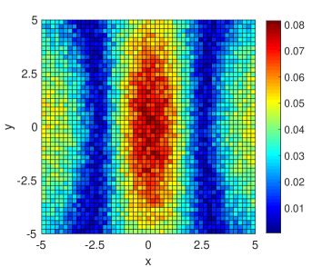
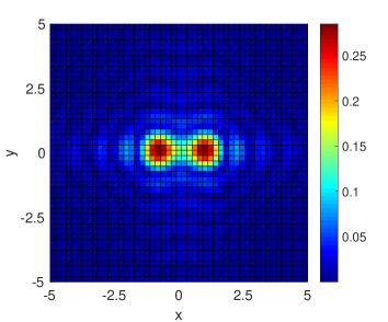
The data propagation process firstly reduces the computational domain for our algorithm and secondly makes the scattered field data look more focused. The latter feature also provides us a reasonable estimate for the location of the target, which is important for the numerical implementation. The data propagation is done using the so called angular spectrum representation, which is a well known technique in optics, see, e.g., [34, Chapter 2]. We also refer to [26, 32, 39], where this process has been exploited for the preprocessing of the experimental data. We display in Figure 1a and Figure 1b the absolute value of the noisy scattered field before and after propagation, respectively. The scatterer in this case consists of two different inclusions as in Figure 4. From the propagated data in Figure 1b we can see two clear peaks at the locations of the inclusions. Comparison of Figure 1a with Figure 1b demonstrates the effectiveness of the data propagation procedure.
7.3 Some computational details
In our computations, and . This means that we have 10 wavenumbers in this interval and from now on we refer to them as for . All computationally simulated data considered below are perturbed by 15 of random artificial noise. More precisely, for each and for each grid point on the measurement plane, the total field data were perturbed as
| (7.1) |
where , and and are random numbers, uniformly distributed on . The norm is taken over the measurement plane. Now assume that is the data obtained after the propagation. More precisely, let be the sum of the propagated scattered field and the incident field. In our algorithm we need the derivative of with respect . We compute it via the finite difference as
Even though the differentiation of the noisy data is an ill-posed problem, this approximation turned out to work well in our numerical implementation. This is partly because the propagated data (Figure 1b) have less noise than the given data (Figure 1a).
Each of our targets to be imaged has its front face at the plane . The backscatter data are measured at the plane on the above mentioned rectangle
| (7.2) |
Next, the backscatter data are propagated to the plane We have noticed that the propagated function is close to zero outside of the rectangle
| (7.3) |
see Figure 1(b). Hence, our computational domain is
| (7.4) |
and we treat as the surface where we have the propagated data.
We have observed that the data propagation process also provides a very good assistance in determining the locations of the targets of interest in the plane. More precisely, the peaks that can be seen in magnitude of the propagated data (Figure 1b), are located exactly at the location of those targets in the plane. Therefore, we can consider our search domain in the plane as
| (7.5) |
where is the number of peaks of on the set and is a neighborhood of the point where attains its th peak. These neighborhoods should not intersect with each other. The truncation value 0.7 was chosen by trial-and-error tests.
When running our algorithm, we do not assume the knowledge of the fact that the front face of any target is located on the plane Still, as we have stated above, we assume the knowledge of some rough estimates of linear sizes of targets of interest. In the direction we search for the target in the range . This search range is motivated by our desired applications for detection of explosives. Indeed, means that the linear size of the target in the direction does not exceed 17.5 cm while linear size of antipersonnel mines and IEDs are typically between 5 cm and 15 cm. Note that similar ranges were used in [26, 32, 39, 38]. Thus, our search domain for the target is . In addition, the right hand side of the formula (5.12) for the function might be complex valued in real computations. Hence, at each iteration we apply the following truncation to the coefficient found by (5.12)
| (7.6) |
Next, the function is smoothed by smooth3 in MATLAB with the Gaussian option. As a result, a new function is obtained. We do not change notation here for brevity. Then, the so obtained function is used for solving the Lippmann-Schwinger equation in the algorithm of Section 5.3.
We solve the Lippmann-Schwinger integral equations (3.10) using a spectral method developed in [29, 42]. This method relies on the periodization technique introduced by Vainikko, which enables the use of the fast Fourier transform in the approximation scheme. For solving the integral equation in our numerical implementation, the domain defined in (7.4) is discretized with the uniform mesh size 0.067 in three dimensions. The code for this numerical solver was done in MATLAB. The boundary value problem (5.5)–(5.6) is solved by the finite element method. We use tetrahedral mesh with a local adaptive refinement for the domain . We coded the numerical solver using FreeFem++ [18], which is a standard software designed with a focus on solving partial differential equations using finite element methods. We refer to www.freefem.org for more information about FreeFem++. All of the figures that are displayed below in this paper were done by visualization tools in MATLAB.
7.4 The first tail function
It is clear from the algorithm (at ) that we use only the gradient , instead of the first tail function . Since we set in Section 4.3, we find the derivatives of by solving the following problem instead of the problem (4.21)
| (7.7) | |||
| (7.8) |
Here, boundary condition (7.8) is from (4.5). Solving (7.7)–(7.8) also helps us avoid the error associated with the numerical differentiation of the first tail function
For the case where only the backscatter data are given on , we simply complete the data on the other parts of the boundary by the incident plane wave , see (7.16). In doing so, we approximately assume that for points located in the domain near . Therefore, this completion leads to the boundary condition for on as
| (7.9) | |||
| (7.10) |
It is seen from condition (7.8) that we need the boundary data for functions , . The derivative with respect to for is calculated as
where is the propagated backscatter field. The function was found by propagating the backscatter field to the two nearby planes and , subtracting the results from each other and dividing by , where we took . Derivatives , , for were calculated using FreeFem++. The propagated data looked very smooth. Again, we have not observed any instabilities.
7.5 The stopping criteria and the choice of the final result
We address in this section the rules for stopping the iterations and the choice of the final result for our algorithm. These rules are guided by the convergence estimate (6.7) of Theorem 6.1 and also by the trial-and-error testing. We recall that estimate (6.7) only claims that functions are located in a sufficiently small neighborhood of the true solution if the number of iterations is not large. However, this theorem does not claim that these functions tend to the exact solution, also see Theorem 2.9.4 in [5] and Theorem 5.1 in [6] for similar results. Therefore, our stopping criteria are derived computationally. We note that the same stopping rules have been used in [32] for the experimental data. For the convenience of the reader we present these rules, which are taken from [32].
We have the stopping criterion for the inner iterations and another one for the outer iterations. Denote by the relative error between the two computed coefficients corresponding by two consecutive inner iterations of the th outer iteration
| (7.11) |
We consider the th and th outer iterations which contains and inner iterations respectively. The sequence of relative errors associated to these two outer iterations is defined by
| (7.12) |
where
The inner iterations with respect to of the th outer iteration in the above algorithm are stopped when either or . We have observed in our numerical experiments that the reconstruction results are essentially the same when we use either 3 or 5 for the maximal number of inner iterations.
Concerning the outer iterations with respect to , it can be seen from the stopping rule for the inner iterations that each outer iteration consists of at least two and at most three inner iterations. Equivalently, the error sequence (7.12) has at least three and at most five elements. We stop the outer iterations if there are two consecutive outer iterations for which their error sequence (7.12) has three consecutive elements less than or equal to . Again, we have no rigorous justification for these stopping rules; they rely on the content of the convergence theorem Theorem 6.1 and on trial-and-error testing. We point out, however, that we do trial-and-error only for one target, which we call “reference target”. Then we use the same rules for all other targets.
We choose the final result for by taking the average of its approximations corresponding to the relative errors in (7.12) that meet the stopping criterion for outer iterations. The computed dielectric constant is determined as the maximal value of the computed ,
| (7.13) |
We have observed in our numerical studies that we need no more than five outer iterations to obtain the final result.
7.6 Numerical examples with complete data
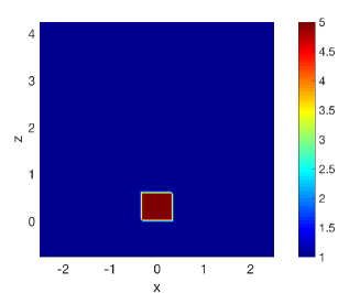
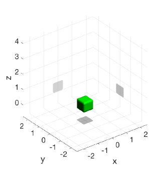
The target we consider for this example is a cube of the size 0.6 defined by
We define the coefficient as
| (7.14) |
We assume that the backscatter data are given on the rectangle (7.2), and on this rectangle the function in (7.1) is replaced with the function . We also assume that the function in (7.1) is given on the part of the domain where and are defined in (7.3) and (7.4) respectively. First, we use the data propagation and obtain the function on the rectangle this way. Next, we consider as the computational domain with the measurement data given on its entire boundary .
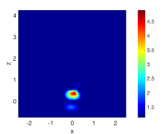
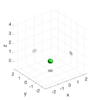
Figure 2 displays the reconstruction result using our algorithm. It can be seen that both the maximal value and the location of the coefficient are well reconstructed. More precisely, for the computed coefficient we have
| (7.15) |
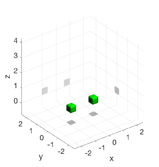
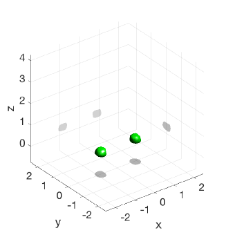
where is defined in (7.13). Hence, it follows from (7.14) and (7.15) that the relative error between the computed maximal value and the exact maximal value of the coefficient is only 2. We visualize the shape and location of the exact target and the reconstructed one using isosurface in MATLAB. The isovalue was chosen as 50 of the maximal value of , and this isovalue is applied to all the other examples in this paper when using isosurface visualization.
7.7 Numerical examples with backscatter data
We examine in this section the performance of our algorithm for the case of backscatter data. This case is of our main interest, which is motivated by our desired application in detecting and identifying of mines and IEDs, where one typically uses only the backscatter measurement in the stand off detection. More precisely, by backscatter data we mean that we are only given the function on the rectangle (7.2). Using the data propagation, we can consider the computational domain in (7.4), where we have the backscatter data on the rectangle defined in (7.3).
Since our method theoretically needs the data on the entire boundary of , we complete the missing data on the other parts of by the corresponding solution of the forward problem in the homogeneous medium, where . In other words, assuming that is the data given on we extend it on the entire boundary as
| (7.16) |
We remark that data completion methods are widely used for inverse problems with incomplete data. The data completion (7.16) is a heuristic technique relying on the successful experiences of [26, 32, 39, 38] when working with globally convergent numerical methods for experimental data.
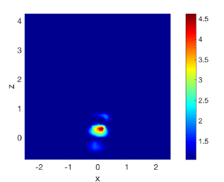
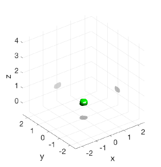
As the first example for the case of backscatter data, we present in Figure 3 the reconstruction results of the coefficient defined in (7.14) for this case. It can be easily seen again that the location is well reconstructed. For the maximal value we have
which implies that the relative error between the exact value and the computed value is 7. Thus, the error has increased from 2% for the case of complete data to 7% for the case of backscatter data only.
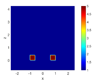
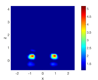
In the second example we consider the target which consists of two similar but separate cubes. The length of the side of each cube is 0.4. The coefficient is defined as
| (7.17) |
| (7.18) |
The reconstruction result for this case is presented in Figure 4. The pictures in the latter figure show a good accuracy of reconstructed locations. Furthermore, we have
This means the relative errors are 4 and for the computed values of the inclusions in and respectively.
7.8 Numerical examples with experimental data
In the last numerical example we address the performance of our algorithm for experimental multi-frequency data. The data were collected by a microwave scattering facility at the University of North Carolina at Charlotte. These measured data are the backscatter signals corresponding to a single incident plane wave . The setting for the measurement is similar to that of the above considered backscatter data case.
It is worth mentioning that the raw data are contaminated by a significant amount of noise, see [32] for a detailed discussion. Furthermore, standard denoising techniques are inapplicable in this case since the raw data have a richer content than the computationally simulated data. Therefore, a heuristic data preprocessing procedure was applied to the raw data in [32]. The preprocessed data were used then as the input for our globally convergent algorithm. The aim of the data preprocessing of [32] is to make the resulting data look somewhat similar to the computationally simulated data. We refer to the paper [32] for all the details about the experimental setup as well as the data preprocessing.
The target here is a tennis ball of the radius 0.31 (see Figure 5(a)). The directly measured average dielectric constant of this target at 3 GHz (or equivalently ) is 3.80, with measurement error given by the standard deviation. This dielectric constant was independently measured by the physicists Professor Michael A. Fiddy and Mr. Steven Kitchin from the Department of Physics and Optical Science at the University of North Carolina Charlotte. Our reconstruction result displayed in Figure 5 indicates that our method accurately reconstructs the location of the target. The maximal value for the computed coefficient is , which is 5.3% error, compared with the direct measurement.
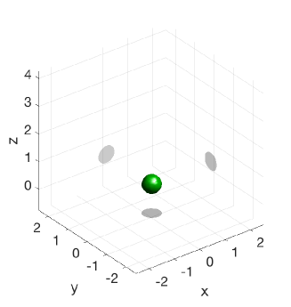
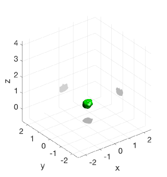
In [32] the above algorithm was tested for five sets of experimental data. Table 1 presents reconstruction results of the value for all five cases; “std.dev” means standard deviation of the error in the a posteriori measured dielectric constants at the frequency of 3 GHz. One can observe that the relative error of the reconstruction is between 2% and 10.3% in cases 1-4, and it is unclear in the case number 5.
| Target | Measured (std. dev.) | Computed | Relative error |
|---|---|---|---|
| A piece of yellow pine | 5.30 (1.6%) | 5.44 | 2.6% |
| A piece of wet wood | 8.48 (4.9%) | 7.60 | 10.3% |
| A geode | 5.44 (1.1%) | 5.55 | 2.0% |
| A tennis ball | 3.80 (13.0%) | 4.00 | 5.2% |
| A baseball | not available | 4.76 | n/a |
8 Summary
We have analytically developed a new numerical method for solving a Coefficient Inverse Problem with single measurement data for the 3D Helmholtz equation. The approximate global convergence of this method is proved. Our targets of interest mimic antipersonnel mines and improvised explosive devices. Numerical results for both computationally simulated and experimental data demonstrate a good accuracy in reconstructed locations and dielectric constants of targets. It is worth mentioning that, in the case of experimental data, this good accuracy is achieved regardless on the above mentioned high level of noise in the data.
Acknowledgments
This work was supported by US Army Research Laboratory and US Army Research Office grant W911NF-15-1-0233 and by the Office of Naval Research grant N00014-15-1-2330. The authors are grateful to Professor Michael A. Fiddy and Mr. Steven Kitchin for their excellent work on collection of experimental data.
References
- [1] A. D. Agaltsov and R.G. Novikov, Riemann-Hilbert approach for two-dimensional flow inverse scattering, J. Math. Phys 55 (2014), 103502.
- [2] H. Ammari, Y. Chow, and J. Zou, Phased and phaseless domain reconstruction in inverse scattering problem via scattering coefficients, SIAM J. Appl. Math. 76 (2016), 1000–1030.
- [3] H. Ammari and H. Kang, Reconstruction of small inhomogeneities from boundary measurements, Lecture Notes in Mathematics, vol. 1846, Springer, 2004.
- [4] A. B. Bakushinsii and M. Y. Kokurin, Iterative Methods for Approximate Solutions of Inverse Problems, Springer, New York, 2004.
- [5] L. Beilina and M. V. Klibanov, Approximate global convergence and adaptivity for coefficient inverse problems, Springer, New York, 2012.
- [6] , A new approximate mathematical model for global convergence for a coefficient inverse problem with backscattering data, J. Inverse and Ill-Posed Problems 20 (2012), 512–565.
- [7] M. Born and E. Wolf, Principles of optics: Electromagnetic theory of propagation, interference and diffraction of light, Cambridge University Press, New York, 1999.
- [8] A. L. Bukhgeim and M. V. Klibanov, Uniqueness in the large of a class of multidimensional inverse problems, Soviet Math. Doklady 17 (1981), 244–247.
- [9] M. Burger and S. Osher, A survey on level set methods for inverse problems and optimal design, European J. of Appl. Math. 16 (2005), 263–301.
- [10] G. Chavent, Nonlinear Least Squares for Inverse Problems: Theoretical Foundations and Step-by-Step Guide for Applications, Scientic Computation, Springer, New York, 2009.
- [11] Y.T. Chow and J. Zou, A numerical method for reconstructing the coefficient in a wave equation, Numerical Methods for PDEs 31 (2015), 289–307.
- [12] D. Colton and A. Kirsch, A simple method for solving inverse scattering problems in the resonance region, Inverse Problems 12 (1996), 383–393.
- [13] D. Colton and R. Kress, Inverse acoustic and electromagnetic scattering theory. second ed., Applied Mathematical Sciences, Springer-Verlag, Berlin, 1998.
- [14] M. de Buhan and M. Kray, A new approach to solve the inverse scattering problem for waves: combining the TRAC and the Adaptive Inversion methods, Inverse Problems 29 (2013), 085009.
- [15] H. W. Engl, M. Hanke, and A. Neubauer, Regularization of Inverse Problems, Kluwer Academic Publishers, Boston, 2000.
- [16] N. Gilbarg and N. S. Trudinger, Elliptic partial differential equations of second order, Springer-Verlag, Berlin Heidelberg New York, 1977.
- [17] A. V. Goncharsky and S. Y. Romanov, Supercomputer technologies in inverse problems of ultrasound tomography, Inverse Problems 29 (2013), 075004.
- [18] F. Hecht, New development in FreeFem++, J. Numerical Mathematics 20 (2012), 251–265.
- [19] K. Ito, B. Jin, and J. Zou, A direct sampling method for inverse electromagnetic medium scattering, Inverse Problems 29 (2013), 095018.
- [20] S. I. Kabanikhin, K. K. Sabelfeld, N.S. Novikov, and M. A. Shishlenin, Numerical solution of the multidimensional Gelfand-Levitan equation, J. Inverse and Ill-Posed Problems 23 (2015), 439–450.
- [21] A. Kirsch, Characterization of the shape of a scattering obstacle using the spectral data of the far field operator, Inverse Problems 14 (1998), 1489–1512.
- [22] M. V. Klibanov, Carleman estimates for global uniqueness, stability and numerical methods for coefficient inverse problems, J. Inverse and Ill-Posed Problems 21 (2013), 477–560.
- [23] M. V. Klibanov, M. A. Fiddy, L. Beilina, N. Pantong, and J. Schenk, Picosecond scale experimental verification of a globally convergent algorithm for a coefficient inverse problem, Inverse Problems 26 (2010), 045003.
- [24] M. V. Klibanov, L. H. Nguyen, A. Sullivan, and L. Nguyen, A globally convergent numerical method for a 1-D inverse medium problem with experimental data, Inverse Problems and Imaging 10 (2016), 1057–1085.
- [25] M. V. Klibanov and V. G. Romanov, Two reconsrtuction procedures for a 3-D phaseless inverse scattering problem for the generalized Helmholtz equation, Inverse Problems 32 (2016), 015005.
- [26] A.E. Kolesov, M. V. Klibanov, L. H. Nguyen, D.-L. Nguyen, and N. T. Thành, Single measurement experimental data for an inverse medium problem inverted by a multi-frequency globally convergent numerical method, preprint, arxiv: 1610.08018, 2016.
- [27] A. V. Kuzhuget, L. Beilina, M. V. Klibanov, A. Sullivan, L. Nguyen, and M. A. Fiddy, Blind backscattering experimental data collected in the field and an approximately globally convergent inverse algorithm, Inverse Problems 28 (2012), 095007.
- [28] O. A. Ladyzhenskaya and N. N. Ural’tseva, Linear and Quasilinear Elliptic Equations, Academic Press, New York, 1968.
- [29] A. Lechleiter and D.-L. Nguyen, A trigonometric Galerkin method for volume integral equations arising in TM grating scattering, Adv. Comput. Math. 40 (2014), 1–25.
- [30] J. Li, H. Liu, and J. Zou, Locating multiple multiscale acoustic scatterers, SIAM Multiscale Model. Simul. 12 (2014), 927–952.
- [31] J. Li, H. Liu and Q. Wang, Enhanced multilevel linear sampling methods for inverse scattering problems, J. Comput. Phys. 257 (2014), 554–571.
- [32] D.-L. Nguyen, M. V. Klibanov, L.H. Nguyen, A. E. Kolesov, M. A. Fiddy, and H. Liu, Numerical solution for a coefficient inverse problem with multi-frequency experimental raw data by a globally convergent algorithm, preprint, arxiv: 1609.03102v2 (2016).
- [33] R. G. Novikov, An iterative approach to non-overdetermined inverse scattering at fixed energy, Sbornik: Mathematics 206 (2015), 120–134.
- [34] L. Novotny and B. Hecht, Principles of nano-optics, 2nd ed., Cambridge University Press, Cambridge, UK, 2012.
- [35] V. G. Romanov, Inverse problems for differential equations with memory, Eurasian J. Math. Comput. Appl. 2 (2014), 51–80.
- [36] J. A. Scales, M. L. Smith, and T. L. Fischer, Global optimization methods for multimodal inverse problems, J. Computational Physics 103 (1992), 258–268.
- [37] M. Soumekh, Syntetic aperture radar signal processing, John Wiley&Sons, New York, 1999.
- [38] , Reconstruction of the refractive index from experimental backscattering data using a globally convergent inverse method, SIAM J. Sci. Comput. 36 (2014), B273–B293.
- [39] N. T. Thành, L. Bellina, M. V. Klibanov, and M. A. Fiddy, Imaging of buried objects from experimental backscattering time dependent measurements using a globally convergent inverse algorithm, SIAM J. Imaging Sciences 8 (2014), 757–786.
- [40] A. N. Tikhonov, A. Goncharsky, V. V. Stepanov, and A. G. Yagola, Numerical methods for the solution of ill-posed problems, Kluwer Academic Publishers Group, Dordrecht, 1995.
- [41] B. R. Vainberg, Asymptotic methods in equations of mathematical physics, Gordon and Breach Science Publishers, New York, 1989.
- [42] G. Vainikko, Fast solvers of the Lippmann-Schwinger equation, Direct and Inverse Problems of Mathematical Physics (Dordrecht) (D.E. Newark, ed.), Int. Soc. Anal. Appl. Comput. 5, Kluwer, 2000, p. 423.
- [43] M. Yamamoto, Carleman estimates for parabolic equations. Topical Review, Inverse Problems 25 (2009), 123013.