Data Compression for the Tomo-e Gozen with Low-rank Matrix Approximation

Abstract

Optical wide-field surveys with a high cadence are expected to create a new field of astronomy, so-called “movie astronomy,” in the near future. The amount of data of the observations will be huge, and hence efficient data compression will be indispensable. Here we propose a low-rank matrix approximation with sparse matrix decomposition as a promising solution to reduce the data size effectively, while preserving sufficient scientific information. We apply one of the methods to the movie data obtained with the prototype model of the Tomo-e Gozen mounted on the 1.0-m Schmidt telescope of Kiso Observatory. Once the full-scale observation of the Tomo-e Gozen commences, it will generate $\sim$30 TB of data per night. We demonstrate that the data are compressed by a factor of about 10 in size without losing transient events like optical short transient point-sources and meteors. The intensity of point sources can be recovered from the compressed data. The processing runs sufficiently fast, compared with the expected data-acquisition rate in the actual observing runs.

=1 The Friends of AASTeX Collaboration

1 Introduction

Optical wide-field surveys with a high cadence has recently emerged as a potential powerful tool to search for optical transient phenomena, and hence to advance our understanding of astrophysics of compact and high-energy objects. The Palomar Transient Factory (PTF) survey with the Palomar 1.2-m Schmidt telescope and the Kiso Supernova Survey (KISS) with the Kiso Wide Field Camera (KWFC) on the Kiso 1.0-m Schmidt telescope have discovered new species of transients with timescales of hours to days from supernovae, novae, to active galactic nuclei (Law et al., 2009; Rau et al., 2009; Sako et al., 2012; Morokuma et al., 2014; Tanaka et al., 2014). High-cadence and wide-field monitoring surveys with the Hyper Suprime-Cam on the Subaru 8.2-m telescope and the Kepler space telescope have successfully obtained transient light-curves originating in shock breakouts of core-collapse supernovae (Tanaka et al., 2016; Garnavich et al., 2016). These results demonstrate importance of high-cadence wide-field survey observations to find rare and short-duration transients. Unsurprisingly, some next-generation survey projects, such as 8.2-m Large Synoptic Survey Telescope (LSST) and Zwicky Transient Facility (ZTF) on the Palomar Schmidt telescope, will be also high-cadence and cover wide fields for galactic, extra-galactic, and solar-system objects (Tyson, 2002; Dekany et al., 2016).

The Tomo-e Gozen is a wide-field CMOS camera on the Kiso 1.0-m Schmidt telescope under development at the time of writing, and is expected to be completed in 2018 (Sako et al., 2016; Ohsawa et al., 2016). It is optimized for movie observations with sub-second to seconds time-resolutions, and once completed, will be capable of taking consecutive frames with a field-of-view of 20 deg² at 2 frames per second (fps) by 84 chips of 2k $\times$ 1k CMOS sensors. The primary objective of observations with the Tomo-e Gozen is to catch rare and fast transient phenomena with a time duration shorter than 10 seconds, such as optical counterparts of fast radio bursts (Keane et al., 2016), giant pulses in millisecond pulsars (Hankins et al., 2003), gamma-ray bursts (Gehrels & Mészáros, 2012), and binary neutron-star mergers (Tanaka & Hotokezaka, 2013). The wide-field movie observation with the Tomo-e Gozen is also ideal for exploring fast moving objects, including near-earth objects and space debris. Such phenomena cannot be explored by the projects using CCDs like PTF, ZTF and LSST, whose time resolutions are 60, 30 and 15 seconds, respectively.

A prototype model of the Tomo-e Gozen with 8 CMOS chips on the Kiso Schmidt telescope (hereafter, the Tomo-e PM; Sako et al., 2016; Ohsawa et al., 2016) has been developed, which has achieved the frame rate of 2-fps so far. We have obtained movie data with a format of FITS cube for each CMOS sensor. A data file typically consists of 400 frames of the same field images with $1136\times 2008$ pixels. The data rate of the Tomo-e PM is $\sim$80 MB s^-1, corresponding to $\sim$3 TB per night. Then, an observation with the complete model of the Tomo-e Gozen will produce a huge amount of data of $\sim$30 TB per night.

It is therefore practically indispensable to compress the data. The data-compression methods have two types: lossless and lossy compressions. Since random noise pervades all the pixels in our case, the former is not effective. For example, the popular lossless tool gzip reduced our movie data by only $\sim$18%. Some lossless methods were proposed for astronomical data sets (Ahnen et al., 2015; Masui et al., 2015). In this paper, we discuss the latter, lossy compression. Various lossy compression algorithms have been proposed for application to astronomical data, such as JPEG2000 (Kitaeff et al., 2015; Vohl, Fluke & Vernardos, 2015), the method using singular value decomposition (SVD; Kolev, Tsvetkova & Tsvetkov, 2012) and wavelet (Belmon et al., 2002). None of them, however, are so far optimized for astronomical “movie” data.

Commercial compression tools for movie data like MPEG4 are readily available. However, we think that at least MPEG method is not appropriate for our data. This method divides images into box regions, and for each box region it compresses the data based on the discrete cosine transform. The level of compression is not uniform, then the fluctuation of pixel intensities becomes different in a source and a background region used for aperture photometry. It results in uncertainty for the photometric intensity of point sources.

Here, we propose an efficient method to compress the movie data for both the space and time domains simultaneously in the lossy-compression manner but without losing signals of transient phenomena, with a calculation speed comparable or faster than the production rate to avoid accumulating yet-unprocessed data.

2 Method

Figure 1: Schematic illustration of data conversion from a cube data to a matrix ($M$), and the matrix decomposition into a low-rank ($L$), sparse ($S$) and noise matrix ($G$). The low-rank matrix is further decomposed by SVD into $L=UDV^{T}$.

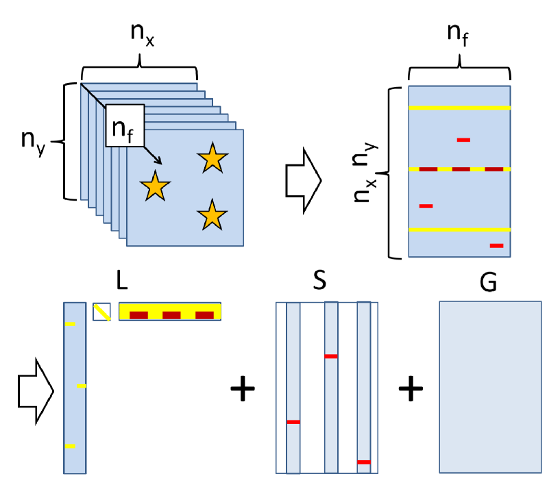
In order to compress the movie data obtained by the Tomo-e Gozen, we choose to use low-rank matrix approximation to reduce the data size without losing transient events. Before applying it, we re-arrange the pixel values contained in a movie data set ($n_{f}$ frames of images with $n_{x}n_{y}$ pixels) into a matrix with $n_{x}n_{y}$ rows and $n_{f}$ columns (Figure 1). Here, $n_{x}$, $n_{y}$, and $n_{f}$ are $1136$, $2008$, and $400$, respectively.

The concept of low-rank matrix approximation with sparse matrix decomposition was originally proposed by Candes et al. (2009). Zhou & Tao (2011) improved the algorithm and the computational speed, and developed GoDec. Since the computational speed is critical in the Tomo-e Gozen application, we develop our method based on GoDec. In our case, an original data matrix $M$ is decomposed into $L+S+G$, where $L$, $S$, and $G$ are a low-rank, sparse, and noise matrix, respectively (See Figure 1), so that the following function is minimized,

$${\rm min}\,\,||G||_{F}={\rm min}\,\,||M-L-S||_{F}$$ (1)

subject to ${\rm rank}(L)<r$ and ${\rm card}(S)<k$, where $||\cdot||_{F}$ denotes the Frobenius norm of a matrix. The parameters $r$ and $k$ control the rank and cardinarity of the low-rank and sparse matrices, respectively.

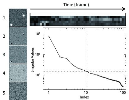
For the low-rank matrix $L$, we check the distribution of singular values, applying singular value decomposition (SVD), as shown in the main panel of Figure 2. The matrix $L$ is expressed as $L=UDV^{T}$, where $U$ and $V$ are orthogonal matrices, and $D$ is a diagonal one. Then, we set the rank of the low-rank matrix by setting zeros for the singular values at indices larger than the rank. Within the sparse matrix $S$, the transient events can be easily extracted, because these events are innately sparse. The time variation of the sky background can be monitored by checking the noise matrix $G$.

After the data matrix $M$ is decomposed into three matrices, $L$, $S$, and $G$, further data processing is necessary, because otherwise the data size would remain three times larger than that of the original data. The low-rank matrix $L$ is easily compressed to three small matrices, as shown in Figure 1. For the sparse matrix $S$, the frames that contain a transient event(s) must be preserved, and the others should be discarded. For this reduction, we use machine-learning methods to select point sources, which has been already established (e.g., Morii et al., 2016, and references therein). For the noise matrix $G$, we obtain some statistics to summarize the distribution of the pixel values and remove the matrix.

Then, the number of pixels can be reduced from the original number of $n_{\rm org}=n_{x}n_{y}n_{f}$ to

$$n_{\rm red}=rn_{x}n_{y}+rn_{f}+r+n_{\rm f,sp}n_{x}n_{y},$$ (2)

where $r$ is a rank of the low-rank matrix $L$, and $n_{\rm f,sp}$ is the number of frames of the sparse matrix $S$, which contains transient events. Typically, $r$ is about $10$ and $n_{\rm f,sp}$ is smaller than 10. Therefore, the reduction factor of the data is $n_{\rm red}/n_{\rm org}\simeq 1/10$.

The original code of GoDec was implemented with MatLab. However, we find the original code to be impractical to apply to our movie data due to the speed of computation and memory consumption. We have rewritten the GoDec code with C++, utilizing OpenBLAS and LAPACK libraries. We use Quick Select, instead of full sorting, to select non-zero elements for a sparse matrix in the GoDec algorithm.

Figure 2: Structure of a low-rank matrix $L$ made by the decomposition. The central panel shows the distribution of singular values of the matrix as a function of the index of the diagonal matrix $D$, obtained by SVD. The five images in the left-hand side show stable point sources, where each image is the decomposed component in the matrix $U$ corresponding to the top five singular values. The upper panel shows the time variation of intensity of these components in the matrix $V$ in gray scale.

3 Application of the proposed method

Figure 3: Example decomposition images for a movie data of the Tomo-e Gozen from two frames (top and bottom rows). Original (denoted as the matrix $M$ in the main text), low-rank ($L$), sparse ($S$), and noise ($G$) images are shown in the four columns in this respective order from the left. A transient point source appears near the center of the image at the time-frame of the top row, as spotted in the original image (a) in contrast to (e) taken in a different frame (bottom row), and as clearly visible in the sparse one (c) in contrast to (g). On the other hand, a line, which is a light trail caused by a meteor, is seen in the second time-frame (bottom row), as in the original image (e) and sparse one (g). These transient events are not recognized in the low-rank images (b, f). Noise images (d, h) do not contain any patterns noticeable.

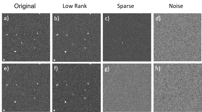
We used a movie dataset of a CMOS sensor for 400 frames obtained with the Tomo-e PM in 2015 December, which contains some transient events lasting for a short duration (Ohsawa et al., 2016). Panels (a) and (e) of Figure 3 show sub-array images with 300 $\times$ 300 pixels in two different time-frames, which contained a transient point source and a meteor, respectively. We applied the decomposition to the data by setting $r=10$ and $k=1\times 10^{8}$. Panels (b, c, d) and (f, g, h) of Figure 3 show the result. A transient was extracted in the sparse matrix $S$ (panel c) and a line generated by a meteor was also detected (panel g). In contrast, the low-rank image $L$ (panels b, f) did not contain any transients. These results confirm that the decomposition was successful.

Figure 4: Distribution of pixel values in the noise image. Histograms for median of pixel intensities of 400 frames are shown. Horizontal and vertical axes are pixel intensity and number of pixels, respectively. The data at zero intensity is not shown.

Figure 5: Relation between pixel intensity of noise frames $G$ and that of original frames $M$.

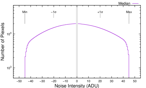
Figure 2 shows the singular values obtained by SVD of the low-rank matrix $L$, suggesting that the rank of 10 is sufficient to preserve the information of stable point sources. Figure 4 shows the pixel values of the noise images $G$. The histograms have a symmetrical shape, no bias and no anomaly structure. In Figure 5, pixel intensities of noise images $G$ were plotted against those of original images $M$, which shows that the intensities of $G$ are independent of the original intensities.

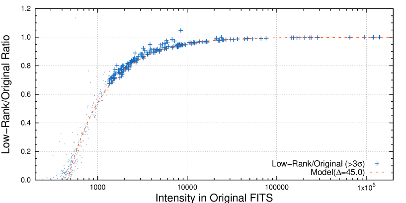
We found that the photometric intensity of point sources in the low-rank matrix $L$ is reduced from the original value, as shown in Figure 6. However, it is possible to recover the original intensity as follows. The photometric intensity of a point source is measured by the standard aperture photometry. To model the distribution of the pixel intensity of a point source, namely point spread function (PSF), we assume a two-dimensional Gaussian function with symmetrical widths for simplicity. That is, the pixel value at a distance $r$ from the center of the point source is given by

$${\rm PSF}(r;d;s)=s\frac{4\ln 2}{\pi d^{2}}\exp\left(-4\ln 2\frac{r^{2}}{d^{2}}\right),$$ (3)

where $d$ and $s$ are the FWHM and the total intensity of a point source, respectively. Then, the total intensity of the pixels within an aperture radius $R$ is

$${I_{\rm enc}}(R;d;s)=s\left[1-\exp\left(-4\ln 2\frac{R^{2}}{d^{2}}\right)\right].$$ (4)

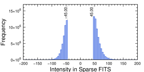
For the residual from the low rank approximation, the pixels lower than a threshold ($\Delta$) are separated into the sparse matrix $S$ or the noise matrix $G$. This applies for the PSF, which results in reducing the aperture size of a point source to $r_{\Delta}$, where ${\rm PSF}(r_{\Delta};d;s)=\Delta$. The $\Delta$ corresponds to the lower threshold of pixel value selected for the sparse matrix $S$. Then, the fraction of the photometric intensity in the low-rank matrix $L$ ($I_{\rm lr}$) to the original one $M$ ($I_{\rm org}$) is approximated by

$$\frac{I_{\rm lr}}{I_{\rm org}}\simeq\frac{{I_{\rm enc}}(r_{\Delta};d;s)}{{I_{\rm enc}}(\infty;d;s)}=1-\frac{\pi d^{2}\Delta}{4\ln 2}\frac{1}{s}.$$ (5)

Figure 6 shows the model curve of $I_{\rm lr}/I_{\rm org}$ for $\Delta=45.0$, obtained from the sparse matrix (Figure 7), and it is in good agreement with the actual data. This implies that the original intensities are recovered well from the low-rank matrix.

Figure 6: Ratio of photometric intensities of point sources in between the low-rank and original frames as a function of the original intensity. Here, the median intensity of 400 frames obtained by photometry for each frame is shown. Cross marks are for sources with a significance of higher than 3 sigma level. Red dashed-line shows the model curve for the ratio (see text).

Figure 7: Distribution of pixel values in the sparse image. The data at zero intensity is not shown.

Next, we examined the sparse matrix, using the transient point source that appeared in the frame of the upper row of Figure 3. We extracted the source from the original $M$ (panel a) and sparse $S$ (panel c) matrices, and found that the intensity of the latter was 74% of the former. This would not be a problem, because we can simply preserve the original image data in any time-frame that is found to contain a transient source(s).

Finally, the processing time of the decomposition was 320 s for the movie data with $1136\times 2008$ pixels and $400$ frames, by setting 10 for the rank of a low-rank matrix, for which we used a budget computer, equipped with a CPU of Intel Xeon Processor E5-1630 (3.70 GHz) consisting of eight cores. The processing time is 1.6 times longer than the duration of observation of 200 s ($0.5$ s $\times$ $400$ frames), which is sufficiently fast for daily observations, as long as one CPU is used for each sensor.

4 Discussion and Conclusion

We have proposed to use the low-rank matrix approximation with sparse matrix decomposition in order to compress the movie astronomical data without losing transient events. Compared with the conventional low-rank matrix approximation with principal component analysis and SVD, our method has an advantage of preserving the transients in the sparse matrices, which is essential for the transient-search project with the Tomo-e Gozen.

Although the value of $k$ was chosen by hand in the current study, it should be chosen so as to maximize the number of the transients which would be selected by the following machine-learning method. If the optimal $k$ is small, further data compression is possible for the sparse matrix $S$ by storing $2k$ numbers for the indices and values of non-zero elements of $S$. In the machine-learning step for the transient detection, either of $S$ and $S+G$ can be used. The latter data may be better, but we have not yet confirmed. We will present these studies in the future.

Our method may miss transient sources which have low significance in each frame but are high significance by stacking multiple frames, if they have time durations of more than a few seconds. In our policy, we discard this type of sources, because the primary objective of the Tomo-e Gozen project is discovering transient sources with a short time scale. In addition, it is possible to keep these transients by stacking raw frames in various time durations like 5, 10, 50 seconds and so on, before applying our compression method.

Now, we are developing both the hardware and software systems of the Tomo-e Gozen survey, including the CMOS camera, data analysis pipeline, and scheduling. Our proposed method has successfully overcome one of the challenges that the project faces. The Tomo-e Gozen will pioneer a new field of astronomy, “movie astronomy.”

References

- Ahnen et al. (2015) Ahnen, M. L., et al., 2015, Astronomy and Computing, 12, 191
- Belmon et al. (2002) Belmon, L., Benoit-Cattin, H., Baskurt, A. & Bougeret, J.-L., 2002, A&A, 386, 1143
- Candes et al. (2009) Candes, E., et al., 2009 http://www-stat.stanford.edu/ candes/papers/RobustPCA.pdf
- Dekany et al. (2016) Dekany, R., et al., 2016, SPIE, 9908, 99085M
- Garnavich et al. (2016) Garnavich, P. M., et al., 2016, ApJ, 820, 23
- Gehrels & Mészáros (2012) Gehrels, N. & Mészáros, P., 2012, Science, 337, 932
- Hankins et al. (2003) Hankins, T. H., et al., 2003, Nature, 422, 141
- Keane et al. (2016) Keane, E. F., et al., 2016, Nature, 530, 453
- Kitaeff et al. (2015) Kitaeff, V. V., et al., 2015, Astronomy and Computing, 12, 229
- Kolev, Tsvetkova & Tsvetkov (2012) Kolev, V., Tsvetkova, K. & Tsvetkov, M., 2012, Publications of the Astronomical Society “Rudjer Boskovic”, 11, 187
- Law et al. (2009) Law, N. M., et al., 2009, PASP, 121, 1395
- Masui et al. (2015) Masui, K., et al. 2015, Astronomy and Comuting, 12, 181
- Morii et al. (2016) Morii, M., et al., 2016 PASJ, accepted (arXiv:1609.03249)
- Morokuma et al. (2014) Morokuma, T., et al. 2014, PASJ, 66, 114
- Ohsawa et al. (2016) Ohsawa, R., et al., 2016, SPIE, 9913, 991339
- Rau et al. (2009) Rau, A., et al. 2009, PASP, 121, 1334
- Sako et al. (2012) Sako, S., et al., 2012, SPIE, 8446, 84466L
- Sako et al. (2016) Sako, S., et al., 2016, SPIE, 9908, 99083P
- Tanaka & Hotokezaka (2013) Tanaka, M. & Hotokezaka, K., 2013, ApJ, 775, 113
- Tanaka et al. (2014) Tanaka, M., et al., 2014, ApJ, 793, L26
- Tanaka et al. (2016) Tanaka, M., et al., 2016, ApJ, 819, 5
- Tyson (2002) Tyson, J. A., 2002, SPIE, 4836, 10
- Vohl, Fluke & Vernardos (2015) Vohl, D., Fluke, C. J., & Vernardos, G., 2015, Astronomy and Computing, 12, 200
- Zhou & Tao (2011) Zhou, T. & Tao, D. 2011, 28th ICML, 33