Path-Complete Graphs and Common Lyapunov Functions

Abstract

A Path-Complete Lyapunov Function is an algebraic criterion composed of a finite number of functions, called its pieces, and a directed, labeled graph defining Lyapunov inequalities between these pieces. It provides a stability certificate for discrete-time switching systems under arbitrary switching.
In this paper, we prove that the satisfiability of such a criterion implies the existence of a Common Lyapunov Function, expressed as the composition of minima and maxima of the pieces of the Path-Complete Lyapunov function. The converse, however, is not true even for discrete-time linear systems: we present such a system where a max-of-2 quadratics Lyapunov function exists while no corresponding Path-Complete Lyapunov function with 2 quadratic pieces exists.
In light of this, we investigate when it is possible to decide if a Path-Complete Lyapunov function is less conservative than another. By analyzing the combinatorial and algebraic structure of the graph and the pieces respectively, we provide simple tools to decide when the existence of such a Lyapunov function implies that of another.

1 Introduction

Switching systems are dynamical systems for which the state dynamics varies between different operating modes. They find application in several applications and theoretical fields, see e.g. PhEsSODT ; AhJuJSRA ; LiMoBPIS ; JuTJSR . They take the form

$$x(t+1)=f_{\sigma(t)}(x(t))$$ (1)

where the state $x(t)$ evolves in $\mathbb{R}^{n}$. The mode $\sigma(t)$ of the system at time $t$ takes value from a set $\{1,\ldots,M\}$ for some integer $M$. Each $i$ mode of the $M$ modes of the system is described by a continuous map $f_{i}(x):\mathbb{R}^{n}\rightarrow\mathbb{R}^{n}$. We assume that $f_{i}(x)=0\Leftrightarrow x=0$ for all modes.

In this paper, we study criteria guaranteeing that the system (1) is stable under arbitrary switching, i.e. where the function $\sigma(\cdot)$, called the switching sequence, takes values in $\{1,\ldots,M\}$ at any time $t$. This analysis can be extended through the more general setting of PhEsSODT (see KoTBWF , (PhEsSODT, , Section 3.5)). We study the following notions of stability, where $x(t,\sigma(\cdot),x_{0})$ is the state of the system (1) at time $t$ with a switching sequence $\sigma(\cdot)$ and an initial condition $x_{0}\in\mathbb{R}^{n}$.

Definition 1

The system (1) is Globally Uniformly Stable if there is a $\mathcal{K}_{\infty}$-function $\alpha:\mathbb{R}^{+}\mapsto\mathbb{R}^{+}$ such that for all $x_{0}\in\mathbb{R}^{n}$, for all switching sequences $\sigma(\cdot)$ and for all $t\geq 0$,

$$\|x(t,\sigma(\cdot),x_{0})\|\leq\alpha(\|x_{0}\|).$$

The system is Globally Uniformly Asymptotically Stable if there is a $\mathcal{KL}$-function $\beta:\mathbb{R}^{+}\times\mathbb{R}^{+}\mapsto\mathbb{R}^{+}$ such that for all $x_{0}\in\mathbb{R}^{n}$, for all switching sequences $\sigma(\cdot)$ and for all $t\geq 0$,

$$\|x(t,\sigma(\cdot),x_{0})\|\leq\beta(\|x_{0}\|,t).$$

The stability analysis of switching systems is a central and challenging question in control (see LiAnSASO for a description of several approaches on the topic). The question of whether or not a system is uniformly globally stable is in general undecidable, even when the dynamics is switching linear (see e.g. JuTJSR ; BlTsTBOA ).

A way to assess stability for switching systems is to use Lyapunov methods, with the drawback that they often provide conservative stability certificates. For example, for linear discrete-time switching systems of the form

$$x(t+1)=A_{\sigma(t)}x(t)$$

it is easy to check for the existence of a common quadratic Lyapunov function (see e.g. (LiAnSASO, , Section II-A)). However, such a Lyapunov function may not exist, even though the system is asymptotically stable (see e.g. LiMoBPIS ; LiAnSASO ). Less conservative parameterizations of candidate Lyapunov functions have been proposed, at the cost of greater computational effort (e.g. for linear switching systems, PaJaAOTJ uses sum-of-squares polynomials, GoHuDMII uses max-of-quadratics Lyapunov functions, and AnLaASCF uses polytopic Lyapunov functions). Multiple Lyapunov functions (see BrMLFA ; ShWiSCFS ; JoRaCOPQ ) arise as an alternative to common Lyapunov functions. In the case of linear systems, the multiple quadratic Lyapunov functions such as those introduced in BlFeSAOD ; DaRiSAAC ; LeDuUSOD ; EsLeCOLS hold special interest as checking for their existence boils down to solving a set of LMIs. The general framework of Path-Complete Lyapunov functions was recently introduced in AhJuJSRA in this context, for analyzing and unifying the approaches cited above.
A Path-Complete Lyapunov function is a multiple Lyapunov function composed of a finite set of pieces $\mathcal{V}=(V_{i})_{i=1,\ldots,N}$, with $V_{i}:\mathbb{R}^{n}\mapsto\mathbb{R}^{+}$, and a set of valid Lyapunov inequalities between these pieces. We assume there exist two $\mathcal{K}_{\infty}$-functions $\alpha_{1}$ and $\alpha_{2}$ such that

$$\forall x\in\mathbb{R}^{n},\,\forall i\in\{1,\ldots,N\},\,\alpha_{1}(\|x\|)\leq V_{i}(x)\leq\alpha_{2}(\|x\|).$$ (2)

These Lyapunov inequalities are represented by a directed and labeled graph $\mathbf{G}=(S,E)$, where $S$ is the set of nodes, and $E$ the set of edges of the graph.There is one node in the graph for each one of the pieces $(V_{i})_{i\in\{1,\ldots,N\}}$ of the Lyapunov function. An edge takes the form $(p,q,w)\in E$, where $p,q\in S$ are respectively its source and destination nodes, and where $w$ is the label of the edge. Such a label is a finite sequence of modes of the system (1) of the form $w=\sigma_{1},\ldots,\sigma_{k}$, with $\sigma_{i}\in\{1,\ldots,M\}$, $1\leq i\leq k$.
An edge as described above encodes the Lyapunov inequality

$$(p,q,w)\in E\Rightarrow\,\forall x\in\mathbb{R}^{n},\,V_{q}(f_{w}(x))\leq V_{p}(x),$$ (3)

where $1\leq p,q\leq P$ and for $w=\sigma_{1}\ldots\sigma_{k}$, with $\sigma_{i}\in\{1,\ldots,M\}$, and $f_{w}=f_{\sigma_{k}}\circ\cdots\circ f_{\sigma_{1}}$ (see Figure 1).

Figure 1: The edge encodes $V_{q}(f_{w}(x))\leq V_{p}(x)$.

By transitivity, paths in the graph $\mathbf{G}$ encode Lyapunov inequalities as well. Given a path $p=(s_{i},s_{i+1},w_{i})_{i=1,\ldots,k}$ of length $k$, we define the label of the path as the sequence $w_{1}\ldots w_{k}$ (i.e. the concatenation of the sequences on the $k$ edges). Such a path encodes the inequality $V_{s_{k+1}}(f_{w_{k}}\circ\cdots\circ f_{w_{1}}(x))=V_{s_{k+1}}(f_{w_{1}\ldots w_{K}}(x))\leq V_{s_{1}}(x)$.
The graph $\mathbf{G}$ defining a Path-Complete Lyapunov function has a special structure, which is defined below and is illustrated in Figure 2.

Definition 2 (Path-Complete Graph)

Consider a directed and labeled graph $\mathbf{G}=(S,E)$, with edges $(s,d,w)\in E$ with $s,d\in S$ and the label $w$ is a finite sequence over $\{1,\ldots,M\}$. The graph is path-complete if for any finite sequence $w$ on $\{1,\ldots,M\}$, there is a path in the graph with a label $w^{\prime}$ such that $w$ is contained in $w^{\prime}$.

(a)

(b)

(c)

Figure 2: The graphs on Figure 2(a) and 2(b) are both path-complete, but the graph on Figure 2(c) is not: there are no paths containing the finite sequence $1212$.

It is shown in (AhJuJSRA, , Theorem 2.4) that a Path-Complete Lyapunov function is indeed a sufficient stability certificate for a switching system. Interestingly, it was recently shown in JuAhACOL that, for linear systems, given a candidate multiple Lyapunov function with quadratic pieces $(V_{i})_{i=1,\ldots,N}$ and with Lyapunov inequalities encoded by a graph $\mathbf{G}$, we cannot conclude stability unless $\mathbf{G}$ is path-complete.

In this paper we first ask a natural question which aims to reveal the connection to classic Lyapunov theory: Can we extract a Common Lyapunov function for the system (1) from a Path-Complete Lyapunov function? We answer this question affirmatively in Section 3, and show that we can always extract a Lyapunov function which is of the form

$$V(x)=\min_{S_{1},\ldots,S_{k}\subseteq S}\left(\max_{s\in S_{i}}V_{s}(x)\right).$$ (4)

Our proof is constructive and makes use of a classical tool from automata theory, namely the observer automaton, to form subsets of nodes in $\mathbf{G}$ that interact in a well defined manner. Next, we show in Subsection 3.2 that the converse does not hold. In detail, we show that there is an asymptotically stable linear system that has a max-of-2-quadratics Lyapunov function, but for which no Path-Complete max-of-2-quadratics Lyapunov function exists. In Section 4 we turn our attention to the problem of deciding a priori when a candidate Path-Complete Lyapunov function provides less conservative stability certificates than another. By analyzing the combinatorial and algebraic structure of the graph and the pieces respectively, we provide tools in Subsections 4.1 and 4.2 to decide when the existence of such a Lyapunov function implies that of another. We illustrate our results numerically in Section 5, and draw the conclusions in Section 6.

2 Preliminaries

Given any integer $M\geq 1$, we write $[M]=\{1,\ldots,M\}$. For the sake of exposition, the directed graphs $\mathbf{G}=(S,E)$ considered herein have the following property: the labels on their edges are of length 1, i.e., for $(i,j,w)\in E$, $w\in[M]$ (which is not the case, e.g. for the graph of Figure 2(b)). It is easy to extend our results to the more general case, as shown in Remark 3.13 later.
We use several tools and concepts from Automata theory (see e.g. (CaLaITDE, , Chapter 2)).

Definition 3 (Connected graph)

The graph $G=(S,E)$ is strongly connected if for all pairs $p,q\in S$, there is a path from $p$ to $q$.

Definition 4 ((Co)-Deterministic Graph)

 
A graph $G=(S,E)$ is deterministic if for all $s\in S$, and all $\sigma\in[M]$, there is at most one edge $(s,q,\sigma)\in E$.
The graph is co-deterministic if for all $q\in S$, and all $\sigma\in[M]$, there is at most one edge $(s,q,\sigma)\in E$.

Definition 5 ((Co)-Complete Graph)

 
A graph $G=(S,E)$ is complete if for all $s\in S$, for all $\sigma\in[M]$ there exists at least one edge $(s,q,\sigma)\in E$.
The graph is co-complete if for all $q\in S$, for all $\sigma\in[M]$, there exists at least one edge $(s,q,\sigma)\in E$.

A (co)-complete graph is also path-complete (AhJuJSRA, , Proposition 3.3). The following allows us to dissociate the graph of a Path-Complete Lyapunov function from its pieces:

Definition 6

Given a system (1), a graph $\mathbf{G}=(S,E)$ and a set of functions $\mathcal{V}=(V_{s})_{s\in S}$, we say that $\mathcal{V}$ is a solution for $\mathbf{G}$, or equivalently, $\mathbf{G}$ is feasible for $\mathcal{V}$, if for all $(p,q,\sigma)\in E$, $V_{q}(f_{\sigma}(x))\leq V_{p}(x).$

Whenever clear from the context, we will make all references to the system (1) implicit.

3 Induced common Lyapunov functions

As defined in the introduction, a Path-Complete Lyapunov function is a type of multiple Lyapunov function with a path-complete graph $\mathbf{G}=(S,E)$ describing Lyapunov inequalities of the form (3) between its pieces $(V_{s})_{s\in S}$.
In this section, we show that we can always extract from a Path-Complete Lyapunov function an induced common Lyapunov function $V(x)$ for the system, that satisfies

$$\forall x\in\mathbb{R}^{n},\,\forall\sigma\in[M],\,V(f_{\sigma}(x))\leq V(x).$$

To do so, we make use of the concept of observer automaton (CaLaITDE, , Section 2.3.4), adapted for directed and labeled graphs (see Remark 1). This graph is defined as follows, and its construction is illustrated in Example 1.

Definition 7 (Observer Graph)

Consider a graph $\mathbf{G}=(S,E)$. The observer graph $O(\mathbf{G})=(S_{O},E_{O})$ is a graph where each state corresponds to a subset of $S$, i.e. $S_{O}\subseteq 2^{S}$, and is constructed as follows:

1. Set $S_{O}:=\{S\}$ and $E_{O}:=\emptyset$.

2. Set $X:=\emptyset$. For each pair $(P,\sigma)\in S_{O}\times[M]$:

   1. Compute $Q:=\cup_{p\in P}\{q|\,(p,q,\sigma)\in E\}.$

   2. If $Q\neq\emptyset$, set $E_{O}:=E_{O}\cup\{(P,Q,\sigma)\}$ then $X:=X\cup Q$.

3. If $X\subseteq S_{O}$, then the observer is given by $O(\mathbf{G})=(S_{O},E_{O})$. Else, set $S_{O}:=S_{O}\cup X$ and go to step 2.

We stress that the nodes of the observer graph $O(\mathbf{G})$ correspond to sets of nodes of the graph $\mathbf{G}$.

Example 1

Consider the graph $\mathbf{G}$ of Figure 3.

Figure 3: A path-complete graph on 4 nodes a,b,c,d and 2 modes, for Example 1.

Figure 4: Observer graph constructed from the graph $\mathbf{G}$ on Figure 3. Each node of the observer $O(\mathbf{G})$ is associated to a set of nodes of $\mathbf{G}$. Notice that the subgraph on the nodes $\{a,c,d\}$, $\{b,d\}$ is itself a complete graph.

The observer graph $O(\mathbf{G})$ is given on Figure 4. The first run through step 2 in Definition 7 is as follows. We have $P=S$. For $\sigma=1$ the set $Q$ is again $S$ itself: indeed, each node $s\in S$ has at least one inbound edge with the label $1$. For $\sigma=2$, since node $b$ has no inbound edge labeled $2$, we get $Q=\{a,c,d\}$. This set is then added to $S_{O}$ in step 3, and the algorithm repeats step 2 with the updated $S_{O}$.

Remark 1

The notion of the observer automaton is presented in (CaLaITDE, , Section 2.3.4). Generally, an automaton is represented by a directed labeled graph with a start state and one or more accepting states. The graphs considered here can be easily transformed into non-deterministic automata by using the so-called $\epsilon$-transitions (see (CaLaITDE, , Section 2.2.4) for definitions). Given a graph $\mathbf{G}=(S,E)$, one can add $\epsilon$-transitions from a new node “a” to all node in S and from all nodes in S to a new node “b”. The generated automaton has the node “a” as the start state and the node “b” as the (single) accepting state.

Observe that in Figure 4 the subgraph of $O(\mathbf{G})$ with two nodes $\{a,c,d\}$ and $\{b,d\}$ is complete and strongly connected. This is due to a key property of the observer graph. We suspect that this property is known (maybe in the automata theory literature) but we have not been able to find a reference until now.

Lemma 1

The observer graph $O(\mathbf{G})=(S_{O},E_{O})$ of any path-complete graph $\mathbf{G}=(S,E)$ contains a unique sub-graph $O^{\star}(\mathbf{G})=(S_{O}^{\star},E_{O}^{\star})$ which is strongly connected, deterministic and complete.

Proof 3.1.

The fact that the observer automaton has a complete, deterministic, connected component is well known (CaLaITDE, , p.90). From Remark 1, the result extends as well to the observer graph.
We prove that this component is unique. For the sake of contradiction, we assume that the observer graph has two complete and deterministic connected components $\mathbf{G}_{1}=(S_{O,1},E_{O,1})$ and $\mathbf{G}_{2}=(S_{O,2},E_{O,2})$. Each component is itself a path-complete graph. Moreover, since they are deterministic and complete, there can never be a path from one component to another.

For any sequence $w$ of elements in $[M]$, there exists a unique path in $O(\mathbf{G})$ with source $S\in S_{O}$ and label $w$. Since $\mathbf{G}_{1}$, $\mathbf{G}_{2}$ are in $O(\mathbf{G})$, then by construction, there exist two sequences $w_{1}$ and $w_{2}$ such that there is a path from $S\in S_{O}$ with label $w_{1}$ that ends in a node in $\mathbf{G}_{1}$ and a path with label $w_{2}$ that ends in a node in $\mathbf{G}_{2}$.

We now consider two paths of infinite length which start from $S\in S_{O}$. The first has the label $w_{1}w_{2}w_{1}\ldots$, illustrated below,

$$S\rightarrow_{w_{1}}P^{1}\rightarrow_{w_{2}}Q^{1}\rightarrow_{w_{1}}P^{2}\rightarrow_{w_{2}}Q^{2}\cdots$$

and visits the nodes $P^{i}\in S_{O,1}$ and $Q^{i}\in S_{O,1}$ after the $ith$ occurrence of the sequences $w_{1}$ and $w_{2}$ respectively. The second path has the label $w_{2}w_{1}w_{2}\ldots$, illustrated below,

$$S\rightarrow_{w_{2}}R^{1}\rightarrow_{w_{1}}T^{1}\rightarrow_{w_{2}}R^{2}\rightarrow_{w_{2}}T^{2}\cdots$$

and visits $R^{i}\in S_{O,2}$ and $T^{i}\in S_{O,2}$ after the $i$-th occurrence of the word $w_{2}$ and $w_{1}$ respectively.

Since $\mathbf{G}_{1}$ and $\mathbf{G}_{2}$ are disconnected, we know that $S\neq P^{i}\neq T^{i}$ and $S\neq Q^{i}\neq R^{i}$. Thus, $P^{1}\subset S$ which in turn implies $Q^{1}\subset R^{1}$, $P^{2}\subset T^{1}$ and so on. More generally, for all $i$, it holds that $Q^{i}\subset R^{i}$ and $P^{i+1}\subset T^{i}$ for all $i$. By symmetry, we have that $T^{i}\subset P^{i}$ and $R^{i+1}\subset Q^{i}$. Consequently, we observe that $|P^{i+1}|\leq|P^{i}|-2$, thus, necessarily, $|P^{|S|-1}|=0$, which is a contradiction since $O(\mathbf{G})$ by construction cannot have empty nodes. Thus, $O(\mathbf{G})$ has a unique, strongly connected, deterministic and complete sub-graph.

We are now in position to introduce our main result.

Theorem 3.2 (Induced Common Lyapunov Function).

Consider Path-Complete Lyapunov function with graph $\mathbf{G}=(S,E)$ and pieces $\mathcal{V}=(V_{s})_{s\in S}$ for the system (1). Let $O^{\star}(\mathbf{G})=(S^{\star}_{O},E^{\star}_{O})$ be the complete and connected sub-graph of the observer $O(\mathbf{G})$. Then, the function

$$V(x)=\min_{Q\in S^{\star}_{O}}\left(\max_{s\in Q}V_{s}(x)\right)$$ (5)

is a Common Lyapunov function for the system (1).

The result is illustrated in the following example, and its proof is provided in Subsection 3.1.

Example 3.3.

Consider the graph $\mathbf{G}$ of Figure 3 and its observer graph in Figure 4. For this observer graph, the unique, strongly connected, deterministic and complete component $O^{\star}(\mathbf{G})=(S_{O}^{\star},E_{O}^{\star})$ has $S_{O}^{\star}=\{\{a,c,d\},\,\{b,d\}\}$. Thus, if $\mathbf{G}$ is feasible for a set of functions $\mathcal{V}=\{V_{a},V_{b},V_{c},V_{d}\}$, from Theorem 3.2, we conclude that

$$V(x)=\min\left\{\max\left(V_{a}(x),V_{c}(x),V_{d}(x)\right),\,\max\left(V_{b}(x),V_{d}(x)\right)\right\}$$ (6)

is a Common Lyapunov function. Figure 5(a) illustrates an example of the level sets of the function (6) when each piece is a quadratic function. Note that this level set is not convex, which shows the expressive power of path-complete criteria. A geometric illustration of the Lyapunov inequalities infered by the graph $\mathbf{G}$, and in particular of the fact that $V(f_{1}(x))\leq V(x)$, is presented in Figure 5(b).

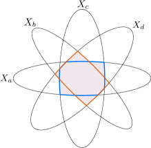
(a) A graphical illustration of the level set of $V$ at Eq. (6) in Example Example 5. The unit sublevel sets $\emph{X}_{s}$, $s\in\{a,b,c,d\}$ of the functions $(V_{s})_{s\in S}$ are ellipsoids. The level set of $V(x)$ is the union of two sets: the set $X_{a}\cap X_{b}\cap X_{c}$ (in blue) and the set $X_{c}\cap X_{d}$ (in orange).

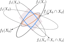
(b) A graphical illustration of the Lyapunov inequalities for Example 5. Let $(X_{s})_{s\in S}$, the level sets of the functions $(V_{s})_{s\in S}$ be such as in Figure 5(a). The image of the set $X_{s}$ set through $f_{1}$ is $f_{1}(X_{s})=\{f_{1}(x),\,x\in X_{s}\}$. From an edge $(s,d,1)\in E$ of the graph $\mathbf{G}$, we can infer that $f_{1}(X_{s})\subseteq X_{d}$ since $V_{s}(x)\geq V_{d}(f_{1}(x))$. We can infer more refined relations by taking several edges. For example, from the edges $(b,a,1)$, $(b,c,1)$, and $(b,d,1)$, we infer that $f_{1}(X_{b})\subseteq X_{a}\cap X_{c}\cap X_{d}$. Taking all edges of the form $(s,d,1)$ into account, we observe that the level set of $V(x)$ (in gray) at Eq. (4) is mapped into itself through $f_{1}$.

Figure 5: Illustrations for Example 2.

3.1 Existence of an induced Common Lyapunov Function

The following results expose relations between two subsets of states of a graph $\mathbf{G}=(S,E)$ that lead to Lyapunov inequalities between the corresponding subsets of pieces of a Path-Complete Lyapunov function. These intermediate results are central to the proof of Theorem 3.2.

Proposition 3.4.

Consider the system (1) and a graph $\mathbf{G}=(S,E)$ which is feasible for a set of functions $(V_{s})_{s\in S}$. Take two subsets $P$ and $Q$ of $S$. If there is a label $\sigma$ such that

$$\forall p\in P,\,\exists q\in Q:\,(p,q,\sigma)\in E,$$ (7)

then

$$\min_{q\in Q}V_{q}(f_{\sigma}(x))\leq\min_{p\in P}{V_{p}(x)}.$$

Proof 3.5.

Take any $x\in\mathbb{R}^{n}$. There exists a node $p^{\star}\in P$ such that $\min_{p\in P}V_{p}(x)=V_{p^{\star}}(x)$. Also, there is at least one edge $(p^{\star},q^{\star},\sigma)\in E$, with $q^{\star}\in Q$. Thus, $V_{q^{\star}}(f_{\sigma}(x))\leq V_{p^{\star}}(x)$ and taking into account that $\min_{q\in Q}V_{q}(f_{\sigma}(x))\leq V_{q^{\star}}(f_{\sigma}(x))$ the result follows.

Proposition 3.4 generalizes the following result, first stated in (AhJuJSRA, , Corollary 3.4).

Corollary 3.6.

If $\mathbf{G}=(S,E)$ is complete and feasible for a set $(V_{s})_{s\in S}$, then $\min_{s\in S}V_{s}(x)$ is a common Lyapunov function for the system (1).

Proof 3.7.

Proposition 3.4 holds here for $P=Q=S$, and all modes $\sigma\in[M]$.

Proposition 3.8.

Consider the system (1) and a graph $\mathbf{G}=(S,E)$ which is feasible for a set of functions $(V_{s})_{s\in S}$. Take two sets of nodes $P$ and $Q$. If there is a label $\sigma$ such that,

$$\forall q\in Q,\exists p\in P:\,(p,q,\sigma)\in E,$$ (8)

then

$$\max_{q\in Q}V_{q}(f_{\sigma}(x))\leq\max_{p\in P}{V_{p}(x)}.$$

Proof 3.9.

Take any $x\in\mathbb{R}^{n}$. There exists a node $q^{\star}\in Q$ such that $\max_{q\in Q}V_{q}(f_{\sigma}(x))=V_{q^{\star}}(f_{\sigma}(x))$. Also, since there exists a node $p^{\star}\in P$ such that $(p^{\star},q^{\star},\sigma)\in E$, it holds that $V_{q^{\star}}(f_{\sigma}(x))\leq V_{p^{\star}}(x)\leq\max_{p\in P}V_{p}(x)$ and the result follows.

Proposition 3.8 generalizes the following result, first stated in (AhJuJSRA, , Corollary 3.5).

Corollary 3.10.

If $\mathbf{G}=(S,E)$ is co-complete and feasible for a set $(V_{s})_{s\in S}$, then $\max_{s\in S}V_{s}(x)$ is a common Lyapunov function for the system.

Proof 3.11.

Proposition 3.8 holds here for $P=Q=S$, and all modes $\sigma\in[M]$.

We are in the position to prove Theorem 3.2.

Proof 3.12 (of Theorem 3.2).

Take a Path-Complete Lyapunov function with a graph $\mathbf{G}=(S,E)$ and pieces $(V_{s})_{s\in S}$. Then, construct the observer graph $O(\mathbf{G})=(S_{O},E_{O})$. By definition, there is an edge $(P,Q,\sigma)\in E_{O}$ if and only if $Q=\cup_{p\in P}\{q|\,(p,q,\sigma)\in E\},$ and therefore, the following property holds for such edges: $\forall q\in Q,\,\exists p\in P$ such that $(p,q,\sigma)\in E$. Consequently, from Proposition 3.8, we have that

$$(P,Q,\sigma)\in E_{O}\Rightarrow\max_{q\in Q}V_{q}(f_{\sigma}(x))\leq\max_{p\in P}{V_{p}(x)}.$$

Therefore, the graph $O(\mathbf{G})$ is feasible for the set of functions $\mathcal{W}=\{W_{P}(x)\}_{P\in S_{O}}$, where

$$W_{P}(x)=\max_{p\in P}V_{p}(x),\quad\forall P\in S_{O}.$$

From Lemma 1, there exists a sub-graph $O^{\star}(\mathbf{G})=(S^{\star}_{O},E^{\star}_{O})$ of $O(\mathbf{G})$ (with $S^{\star}_{O}\subseteq S_{O}$) which is complete and strongly connected. Since $O(\mathbf{G})$ is feasible for $\mathcal{W}$, its subgraph $O^{\star}(\mathbf{G})$ is feasible for the $\{W_{P}\}_{P\in S^{\star}_{O}}$. Finally, since by Lemma 1 $O^{\star}(\mathbf{G})$ is complete, we apply Corollary 3.4 and deduce that the function $W(x)=\min_{P\in S_{O}^{\star}}W_{P}(x)$ is a common Lyapunov function for the system.

Remark 3.13.

Our results extend to graphs $\mathbf{G}=(S,E)$ where the labels are finite sequences of elements in $[M]$ (e.g., as in Figure 2(b), 2c) as follows. One can apply the results on the so-called expanded form of these graphs (AhJuJSRA, , Definition 2.1). The idea there is the following: if an edge $(p,q,w)\in E$ has a label $w=\sigma_{1},\ldots,\sigma_{k}$ of length $k\geq 2$, then it is replaced by a path of length $k$, $(s_{i},s_{i+1},\sigma_{i})_{i=1,\ldots,k}$ where $\sigma_{1}=p$, $\sigma_{k+1}=q$, by adding the nodes $s_{2},\ldots,s_{k}$ to the graph. The expanded form is obtained by repeating the process until all labels in the graph are of size 1 (see Figure 6).

Figure 6: An edge in $\mathbf{G}$ $(i,j,\sigma_{1}\sigma_{2})$ (with label of length 2), is replaced by a path of length 2 in the extended form.

If the graph $\mathbf{G}=(S,E)$ is feasible for a set $\mathcal{V}$, we can always construct a set of functions $\mathcal{W}$ such that the expanded graph $\mathbf{G}_{e}=(S_{e},E_{e})$ of $\mathbf{G}$ is feasible for $\mathcal{W}$. For example, for a path $(s_{i},s_{i+1},\sigma_{i})_{i=1,\ldots,k}$ in the expanded form corresponding to an edge $(p,q,w)$ in $\mathbf{G}$ with $w=\sigma_{1}\ldots\sigma_{k}$, we set $W_{p}=V_{p}$, $W_{q}=V_{q}$, and $W_{s_{i}}(x)=V_{j}(f_{\sigma_{i+1}\ldots\sigma_{k}}(x))$. In Figure 6, we would have $W_{s_{2}}(x)=V_{j}(f_{\sigma_{2}}(x))$.

Remark 3.14.

We can establish a ‘dual’ version of the Theorem 3.2. In specific, given the graph $\mathbf{G}$, we reverse the direction of the edges obtaining a graph $\mathbf{G}^{\top}$, construct its observer $O(\mathbf{G}^{\top})$ and reverse the direction of its edges again, obtaining a graph $O(\mathbf{G}^{\top})^{\top}$. This graph is co-deterministic and contains a unique, strongly-connected, co-complete sub-graph that induces a Lyapunov function of the form

$$V(x)=\max_{S_{1},\ldots,S_{k}\subseteq S}\left(\min_{s\in S_{i}}V_{s}(x)\right),$$

which is, in general, not equal to the common Lyapunov function obtained through Theorem 3.2.

3.2 The converse does not hold

In this subsection we investigate whether or not any Lyapunov function of the form (4) can be induced from a path-complete graph with as many nodes as the number of pieces of the function itself. We give a negative answer to this question by providing a counter example from (GoHuDMII, , Example 11). Consider the discrete-time linear switching system on two modes $x(t+1)=A_{\sigma(t)}x(t)$ with

$$A_{1}=\begin{pmatrix}0.3&1&0\\ 0&0.6&1\\ 0&0&0.7\end{pmatrix},\,A_{2}=\begin{pmatrix}0.3&0&0\\ -0.5&0.7&0\\ -0.2&-0.5&0.7\end{pmatrix}.$$ (9)

The system has a max-of-quadratics Lyapunov function $V(x)=\max\{V_{1}(x),V_{2}(x)\}$, with $V_{i}(x)=\left(x^{\top}Q_{i}x\right)$, $Q_{i}$ being positive definite matrices. An explicit Lyapunov function is given by

$$Q_{1}=\begin{pmatrix}36.95&-36.91&-5.58\\ \cdot&84.11&-38.47\\ \cdot&\cdot&49.32\end{pmatrix},$$

$$Q_{2}=\begin{pmatrix}13.80&-6.69&4.80\\ \cdot&21.87&10.11\\ \cdot&\cdot&82.74\end{pmatrix}.$$

We first observe that these quadratic functions cannot be the solution of a path-complete stability criterion for our example. Indeed, let us draw the graph of all the valid Lyapunov inequalities. More precisely, we define the graph $\mathbf{G}=(\{1,2\},E)$ with two nodes and

$$(i,j,\sigma)\in E\Leftrightarrow A_{\sigma}^{\top}Q_{j}A_{\sigma}-Q_{i}\preceq 0,$$ (10)

i.e. the matrix $A_{\sigma}^{\top}Q_{j}A_{\sigma}-Q_{i}$ is negative semi-definite. The graph obtained is presented on Figure 7. This graph is not path-complete, and thus we cannot form a Common Lyapunov Function, as done in the previous section, with these two particular pieces.

Figure 7: The valid Lyapunov inequalities for the quadratic functions for the system and the Lyapunov function in (GoHuDMII, , Example 11) are represented by the graph above. The graph is not path complete.

However, we can go further and investigate whether another pair of quadratic functions would exist, which we could find by solving a path-complete criterion, and such that their maximum would be a valid CLF. Recall that co-complete graphs induce Lyapunov functions of the form $\max_{v\in S}V_{v}(x)$ (see Corollary 3.10).

Proposition 3.15.

Consider the discrete-time linear system with two modes (9). The system does not have a Path-Complete Lyapunov function with quadratic pieces defined on co-complete graphs with 2 nodes.

Proof 3.16.

From Definition 5, there is a total of $16$ graphs that are co-complete and consist of two nodes and four edges (1 edge per mode and per state). We do not examine co-complete graphs with more than four edges since satisfaction of the Lyapunov conditions for these graphs would imply that of the conditions for at least one graph with four edges.
For each graph, the existence of a feasible set of quadratic functions can be tested by solving the LMIs (10).
For the system under consideration, none of the 16 sets of LMIs have a solution. Thus, no induced Lyapunov function of the type $\max\{V_{1}(x),V_{2}(x)\}$ exists.

Remark 3.17.

In fact, for the Proof of Proposition 3.15, we need only to test four graphs. Three are co-complete with two nodes:

$$G_{1} =(\{a,b\},\{(a,a,1),(a,b,1),(b,a,2),(b,b,2)\}),$$

$$G_{2} =(\{a,b\},\{(a,a,1),(a,b,1),(a,b,2),(b,a,2)\}),$$

$$G_{3} =(\{a,b\},\{(a,a,2),(a,b,1),(a,b,2),(b,a,1)\}),$$

and the last one corresponds to the common quadratic Lyapunov function

$$G_{4} =(\{a\},\{(a,a,1),(a,a,2)\}).$$

One can show that each one of the $13$ remaining co-complete graph is equivalent to one of these four graphs (either isomorphic, or satisfying the conditions of Corollary 4.24 which will be presented later).

Remark 3.18.

For linear systems and for the assessment of asymptotic stability, Path-Complete Lyapunov functions have been shown to be universal. In particular, LeDuUSOD show this for the so-called Path-Dependent Lyapunov functions, which are Path-Complete Lyapunov functions with a particular choice of complete graphs, specifically, the so-called De Bruijn graphs.
The system concerned by Proposition 3.15 is actually asymptotically stable (see GoHuDMII ). The interest of Proposition 3.15 lies in the fact that there do not exist necessarily Path-Complete Lyapunov functions with the same number of pieces as a $\max$-type common Lyapunov function. This is a limitation induced from the combinatorial structure of the Path-Complete Lyapunov function.

The proof of Proposition 3.15 highlights an interesting fact. Several different path-complete graphs may induce the same common Lyapunov function (4). However, the strength of the stability certificate they provide may differ. This has a practical implication: if we are given a system of the form (1), it is unclear which graph $\mathbf{G}$ we should use to form a Path-Complete Lyapunov function for some number of pieces satisfying a given template (e.g., quadratic functions). We present, in Section 4, a first attempt for analyzing the relative strength of Path-Complete Lyapunov functions based on their graphs and the algebraic properties of the set of functions defining their pieces.

4 The Partial order on
Path-Complete graphs

In this section, we provide tools for establishing an ordering between Lyapunov functions defined on general path-complete graphs, extending the work of (AhJuJSRA, , Section 4.2) on complete graphs. In the following definition, we introduce $\mathcal{U}$ as a template or family of functions to which the pieces of Path-Complete Lyapunov functions belong. For example, $\mathcal{U}$ could be the set of quadratic functions: $\mathcal{U}=\{x\mapsto x^{\top}Qx,\,Q\succ 0\}$. We assume that (2) holds for any finite subset of $\mathcal{U}$.

Definition 4.19.

(Ordering). For two path-complete graphs $\mathbf{G}_{1}=(S_{1},E_{1})$, $\mathbf{G}_{2}=(S_{2},E_{2})$ and a template $\mathcal{U}$, we write $\mathbf{G}_{1}\leq_{\mathcal{U}}\mathbf{G}_{2}$ if the existence of a Path-Complete Lyapunov function on the graph $\mathbf{G}_{1}$ with pieces $(V_{s})_{s\in S_{1}}$, $V_{s}\in\mathcal{U}$ implies that of a Path-Complete Lyapunov function on the graph $\mathbf{G}_{2}$ with pieces $(W_{s})_{s\in S_{2}}$, $W_{s}\in\mathcal{U}$.

For each family of functions $\mathcal{U}$, this defines a partial order on path-complete graphs. A minimal element of the ordering, independent of the choice of $\mathcal{U}$, is given by (see Figure 2(a) for $M=2$)

$$\mathbf{G}^{\star}=(\{a\},\{(a,a,\sigma)_{\sigma\in[M]}\}).$$ (11)

A Path-Complete Lyapunov function on this graph corresponds to the existence of a common Lyapunov function from $\mathcal{U}$ for the system. Thus, $\mathbf{G}^{*}\leq_{\mathcal{U}}\mathbf{G}$ for any $\mathcal{U}$.

Remark 4.20.

We highlight that the properties of the set $\mathcal{U}$ influence the ordering relation defined in Definition 4.19. For example, if $\mathcal{U}$ is a singleton, then it is not difficult to see that $\mathbf{G}_{1}\leq_{\mathcal{U}}\mathbf{G}_{2}$ for any two path-complete graphs. From Theorem 3.2, one can show that this holds as well for a set $\mathcal{U}$ closed under $\min$ and $\max$ operations.

4.1 Bijections between sets of states

We present a sufficient condition under which a graph $\mathbf{G}$ satisfies $\mathbf{G}\leq_{\mathcal{U}}\mathbf{G}^{*}$. It is similar in nature to those of Subsection 3.1, and requires as well that the set $\mathcal{U}$ is closed under addition, an algebraic property satisfied, e.g., by the set of quadratic functions.

Proposition 4.21 (Bijection).

Consider a graph $\mathbf{G}=(S,E)$ feasible for a set of functions $(V_{s})_{s\in S}$. Take two subsets $P$ and $Q$ of $S$. If for $\sigma\in[M]$, there is a subset $E^{\prime}$ of $E$ such that,

$$\forall p\in P,\exists!\,q\in Q:(p,q,\sigma)\in E^{\prime},$$

$$\forall q\in Q,\exists!\,p\in P:(p,q,\sigma)\in E^{\prime},$$

then

$$\sum_{q\in Q}V_{q}(f_{\sigma}(x))\leq\sum_{p\in P}V_{p}(x),\,\forall x\in\mathbb{R}^{n}.$$

Proof 4.22.

The result is obtained by first enumerating the $|{P}|=|{Q}|$ Lyapunov inequalities encoded in $E^{\prime}$, and then summing them up.

Example 4.23.

Consider the graphs $\mathbf{G}_{1}=(S_{1},E_{1})$ and $\mathbf{G}_{2}=(S_{2},E_{2})$ of Figure 8(a) and 8(b) respectively.

(a)

(b)

Figure 8: Example 4.1, the graph $\mathbf{G}_{1}$ (8a) and the graph $\mathbf{G}_{2}$ (8b).

Observe that in $\mathbf{G}_{1}$, if we take the two subsets of nodes $R_{1}=\{a,b\}$ and $R_{2}=\{a,c\}$, then we have that Proposition 4.21 holds for $P=Q=R_{1}$ and $\sigma=1$; $P=Q=R_{2}$ and $\sigma=2$; $P=R_{1},Q=R_{2}$ and $\sigma=1$; and $P=R_{2},Q=R_{1}$ and $\sigma=2$.
Putting together these new Lyapunov inequalities, this allows us to conclude that if $\{V_{a},V_{b},V_{c}\}$ is a solution for $\mathbf{G}_{1}$, then $W_{a^{\prime}}=V_{a}+V_{b}$ and $W_{b^{\prime}}=V_{a}+V_{c}$ is a solution for $\mathbf{G}_{2}$. Thus, if $\mathcal{U}$ is closed under addition, then it follows that $\mathbf{G}_{1}\leq_{\mathcal{U}}\mathbf{G}_{2}$.

Corollary 4.24.

For a graph $\mathbf{G}=(S,E)$, if for all $\sigma\in[M]$, there exists a subset $E_{\sigma}\subset E$ such that

$$\forall p\in S,\exists!\,q\in S:(p,q,\sigma)\in E_{\sigma},$$

$$\forall q\in S,\exists!\,p\in S:(p,q,\sigma)\in E_{\sigma},$$

then if $\mathbf{G}$ is feasible for $(V_{s})_{s\in S}$, the sum $\sum_{s\in S}V_{s}$ is a common Lyapunov function for the system.

Proof 4.25.

Proposition 4.21 holds for $P=Q=S$ and all $\sigma\in[M]$.

Example 4.26.

Consider the graph $\mathbf{G}$ of Figure 9 on four nodes and two modes. If $\mathbf{G}$ is feasible for a set $\{V_{a},V_{b},V_{c},V_{d}\}$, then the system has a common Lyapunov function given by $V_{a}+V_{b}+V_{c}+V_{d}$.

Figure 9: A graph $\mathbf{G}$ whose feasibility implies that of $\mathbf{G}^{\star}$ (Example 4.26).

Taking $\mathcal{U}$ as the set of quadratic functions for example, we have $\mathbf{G}\leq_{\mathcal{U}}\mathbf{G}^{\star}$.

4.2 Ordering by simulation

This next criterion for ordering is actually independent of the choice of $\mathcal{U}$. It is inspired by the concept of simulation between two automata (CaLaITDE, , pp. 91–92).

Definition 4.27.

(Simulation) Consider two path-complete graphs $\mathbf{G}_{1}=(S_{1},E_{1})$ and $\mathbf{G}_{2}=(S_{2},E_{2})$ with a same labels $[M]$. We say that $\mathbf{G}_{1}$ simulates $\mathbf{G}_{2}$ if there exists a function $F(\cdot):S_{2}\rightarrow S_{1}$ such that for any edge $(s_{2},d_{2},\sigma)\in E_{2}$ there exists an edge $(s_{1},d_{1},\sigma)\in E_{1}$ with $F(s_{2})=s_{1}$, $F(d_{2})=d_{1}$.

Remark 4.28.

The notion of simulation we use here is actually stronger than the classical one defined for automata, which defines a relation between the states of the two automata rather than a function.

Proposition 4.29.

Consider two graphs $\mathbf{G}_{1}=(S_{1},E_{1})$ and $\mathbf{G}_{2}=(S_{2},E_{2})$. If $\mathbf{G}_{1}$ is feasible for $(V_{s})_{s\in S_{1}}$, and $\mathbf{G}_{1}$ simulates $\mathbf{G}_{2}$ through the function $F:S_{2}\rightarrow S_{1}$, then $\mathbf{G}_{2}$ is feasible for $(W_{s})_{s\in S_{2}}$, with

$$W_{s}=V_{F(s)},\quad\forall s\in S_{2}.$$

Proof 4.30.

Taking any edge $(s,d,\sigma)\in E_{2}$, we get

$$W_{d}(f_{\sigma}(x))=V_{F(d)}(f_{\sigma}(x))\leq V_{F(s)}(x)=W_{s}(x).$$

Example 4.31.

Consider the graphs on three modes $\mathbf{G}_{1}=(S_{1},E_{1})$ and $\mathbf{G}_{2}=(S_{2},E_{2})$ on three modes with the first depicted on Fig. 10(a) and the second on Fig. 10(b). Proposition 4.29 applies here with $F(\cdot):S_{2}\rightarrow S_{1}$ defined as $F(a^{\prime})=a$, $F(b^{\prime}_{1})=F(b^{\prime}_{2})=b$, $F(c^{\prime})=c$.

(a) Graph $\mathbf{G}_{1}$ for Example 10.

(b) Graph $\mathbf{G}_{2}$ for Example 10.

Figure 10: $\mathbf{G}_{1}$ simulates $\mathbf{G}_{2}$.

5 Example and experiment

In this section, we provide an illustration of our results. First, we present a practically motivated example, where we extract a common Lyapunov function from a Path-Complete Lyapunov function for a given discrete-time linear switching systems on three modes. We next present a numerical experiment comparing the performance of three particular path-complete graphs on a testbench of randomly generated systems, similar to that presented in (AhJuJSRA, , Section 4).

Our focus is on linear switching systems, and Path-Complete Lyapunov functions with quadratic pieces. The existence of such Lyapunov functions can then be checked by solving the LMIs (10).

5.1 Extracting a Common Lyapunov function.

The scenario considered here is similar to that of (PhEsSODT, , Section 4), and deals with the stability analysis of closed-loop linear time-invariant systems subject to failures in a communication channel of a networked control system (see e.g. JuHeCOLS for more on the topic). We are given a linear-time invariant system of the form $x(t+1)=(A+BK)x(t)$, with

$$A=\begin{pmatrix}0.97&0.58\\ 0.17&0.5\end{pmatrix},\,B=\begin{pmatrix}0\\ 1\end{pmatrix},K=\begin{pmatrix}-0.55,0.24\end{pmatrix}.$$

When a communication failure occurs, no signal arrives at the plant, and the control input is automatically set to zero. In this case, the communication channel needs to be fixed before any feedback signal can reach the plant. In order to prevent the impact of failures, periodic inspections of the channel are foreseen every M steps. However, the inspection of the communication channel is costly, and we would like to compute the largest $M$ such that an inspection of the plant at every $M$ steps is sufficient to ensure its stability.
Given $M\geq 1$, we model the failing plant as a switching system with $M$ modes:

$$x(t+M)=\tilde{A}_{\sigma(t)}x(t),$$ (12)

where $\sigma\in\{1,\ldots,M\}$ and $\tilde{A}_{\sigma}=A^{\sigma-1}(A+BK)^{M-\sigma+1}$. In other words, for $\sigma(t)=k$, the communication channel will function properly from time $t$ up until time $t+(M-k)$ included, and will then be down from time $t+(M-k)+1$ until time $t+M-1$ included. This assumes that the channel always functions properly at the very first step after inspection.

For $M=1$, the stability analysis is direct as $(A+BK)$ is stable. For $M=2$ we can verify that the system has a Path-Complete Lyapunov function for the graph of Figure 8(b). The case $M=4$ is straightforward: the matrix $\tilde{A}_{4}=A^{3}(A+BK)$ is unstable, and thus the system is unstable in view of Definition 1.

For the case when $M=3$, we verify numerically that the system does not have a common quadratic Lyapunov function. Furthermore,it does not have a Path-Complete Lyapunov function with quadratic pieces for $\mathbf{G}_{2}$ on four nodes represented at Figure 10(b). Note that since $\mathbf{G}_{1}$ simulates $\mathbf{G}_{2}$ (see Example 10), this allows us to conclude that $\mathbf{G}_{1}$ will not provide us with a Path-Complete Lyapunov function as well, or that would contradict Proposition 4.29.

Figure 11: Graph $\mathbf{G}_{3}$, for the example of Section 5.

However, the graph $\mathbf{G}_{3}$ on four nodes represented at Figure 11, which alike $\mathbf{G}_{2}$ is simulated by $\mathbf{G}_{1}$, does provide us with a Path-Complete Lyapunov function with four quadratic pieces. By applying Theorem 3.2, after computing the observer graph of $\mathbf{G}_{3}$ (see Figure 12), we obtain a common Lyapunov function $V(x)$ of the form (4) for the system,

$$V(x)=\min_{S\in\{\{a,c\},\,\{b,c\},\,\{b,d\}\}}\left(\max_{s\in S}V_{s}(x)\right).$$

whose level set is represented in Figure 13.

Figure 12: Observer graph for $\mathbf{G}_{3}$ at Figure 11. The subgraph on the nodes $\{a,c\},\,\{b,c\}$ and $\{b,d\}$ is complete.

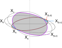
Figure 13: The sets $X_{a}$, $X_{b}$, $X_{c}$ and $X_{d}$ are the level sets of the pieces of the Path-Complete Lyapunov function for the system (12). We let $X_{\{i,j\}}=X_{i}\cap X_{j}$. The grey set is a level set of a Common Lyapunov function for the system, obtained from the Path-Complete Lyapunov function through Theorem 3.2.

5.2 Numerical experiment.

In Section 13 we presented a linear switching system for which a Path-Complete Lyapunov function with quadratic pieces exists for the graph $\mathbf{G}_{3}$ of Figure 11, but not for $\mathbf{G}_{1}$ of Figure 10(a) and $\mathbf{G}_{2}$ of Figure 10(b). However for another system with three modes, it could be $\mathbf{G}_{2}$ that provides a stability certificate, and not $\mathbf{G}_{3}$. It is therefore natural to ask which situation is the more likely to occur for random systems.

To this purpose we generate triplets of random matrices $M=\{A_{1},A_{2},A_{3}\}$. Then, for each triplet and for each graph $\mathbf{G}_{i}=(S_{i},E_{i}),\,i=1,2,3$, we compute the quantity

$$\gamma_{i}=\sup_{\gamma,\,(Q_{s}\succ 0)_{s\in S_{i}}}\gamma:\left\{\begin{aligned} &\forall(s,d,\sigma)\in E_{i},\\ &\gamma^{2}A_{\sigma}^{\top}Q_{d}A_{\sigma}-Q_{s}\preceq 0,\end{aligned}\right.,$$

that is, the higher number $\gamma$ such that $\mathbf{G}_{i}$ provides a stability certificate for the system $x(t+1)=\gamma A_{\sigma(t)}x(t),\,A_{\sigma}\in M$. For a given triplet $M=\{A_{1},A_{2},A_{3}\}$, the fact that $\gamma_{i}\geq\gamma_{j}$, $i\neq j$, translates as follows: whenever $\mathbf{G}_{j}$ induces a Lyapunov function so does $\mathbf{G}_{i}$. Note that it is possible that for a triplet $M$, we get $\gamma_{i}=\gamma_{j}$.

The results are presented in the Venn diagram of Figure 14 for 10800 triplets with matrices of dimension $n=2$.

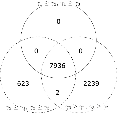
Figure 14: Visualization of the outcome of the numerical experiment. As expected from the theory, whenever $\mathbf{G}_{1}$ provides a stability certificate, so do $\mathbf{G}_{2}$ and $\mathbf{G}_{3}$. There are more systems for which $\mathbf{G}_{3}$ provides a certificate and not $\mathbf{G}_{2}$ than the reverse. Interestingly, it appears unusual that a system has a stability certificate for both $\mathbf{G}_{2}$ and $\mathbf{G}_{3}$, and not $\mathbf{G}_{1}$.

We observe that the results are in agreement with Proposition 4.29, when $\mathbf{G}_{1}$ provides a stability certificate, so do $\mathbf{G}_{2}$ and $\mathbf{G}_{3}$. Also, it appears that a random triplet of matrices is more likely to have a Lyapunov function induced by $\mathbf{G}_{3}$ ($\sim 94\%$ of the cases) rather than by $\mathbf{G}_{2}$ ($\sim 79\%$ of the cases). Interestingly, there appear to be very few instances for which $\gamma_{2}=\gamma_{3}>\gamma_{1}$, which deserves further attention.

6 Conclusion

Path-complete criteria are promising tools for the analysis of hybrid or cyber-physical systems. They encapsulate several powerful and popular techniques for the stability analysis of swiching systems. However, their range of application seems much wider, as for instance 1) they can handle switching nonlinear systems as well, as it is the case herein, 2) they are not limited to LMIs and quadratic pieces and 3) they have been used to analyze systems where the switching signal is constrained PhEsSODT . On top of this, we are investigating the possibility of studying other problems than stability analysis with these tools.

However, already for the simplest particular case of multiple quadratic Lyapunov functions for switching linear systems, many questions still need to be clarified. In this paper we first gave a clear interpretation of these criteria in terms of common Lyapunov function: each criterion implies the existence of a common Lyapunov function which can be expressed as the minimum of maxima of sets of functions. We then studied the problem of comparing the (worst-case) performance of these criteria, and provided two results that help to partly understand when/why one criterion is better than another one. We leave open the problem of deciding, given two path-complete graphs, whether one is better than the other.

References

- [1] Amir Ali Ahmadi, Raphaël M Jungers, Pablo A Parrilo, and Mardavij Roozbehani. Joint spectral radius and path-complete graph lyapunov functions. SIAM Journal on Control and Optimization, 52(1):687–717, 2014.
- [2] Nikolaos Athanasopoulos and Mircea Lazar. Alternative stability conditions for switched discrete time linear systems. In IFAC World Congress, pages 6007–6012, 2014.
- [3] Pierre-Alexandre Bliman and Giancarlo Ferrari-Trecate. Stability analysis of discrete-time switched systems through lyapunov functions with nonminimal state. In Proceedings of IFAC Conference on the Analysis and Design of Hybrid Systems, pages 325–330, 2003.
- [4] Vincent D Blondel and John N Tsitsiklis. The boundedness of all products of a pair of matrices is undecidable. Systems & Control Letters, 41(2):135–140, 2000.
- [5] Michael S Branicky. Multiple lyapunov functions and other analysis tools for switched and hybrid systems. IEEE Transactions on Automatic Control, 43(4):475–482, 1998.
- [6] Christos G Cassandras and Stephane Lafortune. Introduction to discrete event systems. Springer Science & Business Media, 2009.
- [7] Jamal Daafouz, Pierre Riedinger, and Claude Iung. Stability analysis and control synthesis for switched systems: a switched lyapunov function approach. IEEE Transactions on Automatic Control, 47(11):1883–1887, 2002.
- [8] Ray Essick, Ji-Woong Lee, and Geir E Dullerud. Control of linear switched systems with receding horizon modal information. IEEE Transactions on Automatic Control, 59(9):2340–2352, 2014.
- [9] Rafal Goebel, Tingshu Hu, and Andrew R Teel. Dual matrix inequalities in stability and performance analysis of linear differential/difference inclusions. In Current trends in nonlinear systems and control, pages 103–122. Springer, 2006.
- [10] Mikael Johansson, Anders Rantzer, et al. Computation of piecewise quadratic lyapunov functions for hybrid systems. IEEE transactions on automatic control, 43(4):555–559, 1998.
- [11] Raphaël Jungers. The joint spectral radius. Lecture Notes in Control and Information Sciences, 385, 2009.
- [12] Raphael M Jungers, Amirali Ahmadi, Pablo Parrilo, and Mardavij Roozbehani. A characterization of lyapunov inequalities for stability of switched systems. arXiv preprint arXiv:1608.08311, 2016.
- [13] Raphael M Jungers, WPMH Heemels, and Atreyee Kundu. Observability and controllability analysis of linear systems subject to data losses. arXiv preprint arXiv:1609.05840, 2016.
- [14] Victor Kozyakin. The Berger–Wang formula for the markovian joint spectral radius. Linear Algebra and its Applications, 448:315–328, 2014.
- [15] Ji-Woong Lee and Geir E Dullerud. Uniform stabilization of discrete-time switched and markovian jump linear systems. Automatica, 42(2), 205-218, 2006.
- [16] Daniel Liberzon and Stephen A Morse. Basic problems in stability and design of switched systems. IEEE Control Systems Magazine, 19(5):59–70, 1999.
- [17] Hai Lin and Panos J Antsaklis. Stability and stabilizability of switched linear systems: a survey of recent results. IEEE Transactions on Automatic control, 54(2):308–322, 2009.
- [18] Pablo A Parrilo and Ali Jadbabaie. Approximation of the joint spectral radius using sum of squares. Linear Algebra and its Applications, 428(10):2385–2402, 2008.
- [19] Matthew Philippe, Ray Essick, Geir Dullerud, and Raphaël M Jungers. Stability of discrete-time switching systems with constrained switching sequences. Automatica, 72:242–250, 2016.
- [20] Robert Shorten, Fabian Wirth, Oliver Mason, Kai Wulff, and Christopher King. Stability criteria for switched and hybrid systems. SIAM review, 49(4):545–592, 2007.