Dichroic subjettiness ratios to distinguish colour flows in boosted boson tagging

Abstract

$N$-subjettiness ratios are in wide use for tagging heavy boosted objects, in particular the ratio of 2-subjettiness to 1-subjettiness for tagging boosted electroweak bosons. In this article we introduce a new, dichroic ratio, which uses different regions of a jet to determine the two subjettiness measures, emphasising the hard substructure for the 1-subjettiness and the full colour radiation pattern for the 2-subjettiness. Relative to existing $N$-subjettiness ratios, the dichroic extension, combined with SoftDrop (pre-)grooming, makes it possible to increase the ultimate signal significance by about $25\%$ (for $2\,\text{TeV}$ jets), or to reduce non-perturbative effects by a factor of $2{-}3$ at $50\%$ signal efficiency while maintaining comparable background rejection. We motivate the dichroic approach through the study of Lund diagrams, supplemented with resummed analytical calculations.

1 Introduction

With the increasingly high-energy scales probed by the Large Hadron Collider (LHC), massive electroweak bosons ($H/Z/W$) and top quarks are often produced with a transverse momentum much larger than their mass. In this boosted regime, when they decay hadronically, they are reconstructed as single jets that have to be separated from the much more common quark- and gluon-initiated jets. Over the past few years, several techniques relying on jet substructure, i.e. on the internal dynamical properties of jets, have been devised in order to achieve this task. These techniques are now routinely used in LHC analyses and new-physics searches.

There are three common families of methods used to separate boosted heavy objects from standard QCD jets: (i) taggers, which impose that a jet contain two hard cores (or three for a top-quark), a situation more common in signal jets than in QCD jets which are dominated by soft-gluon radiation; an increasingly widespread technique for tagging is the modified MassDrop tagger (mMDT) Butterworth:2008iy ; Dasgupta:2013ihk and its generalisation, SoftDrop Larkoski:2014wba , which will be our chosen tools here; (ii) radiation constraints, which constrain soft-gluon radiation inside jets, expected to be larger in QCD jets than in colourless weak-boson decays; a widespread way of applying radiation constraints is to cut on jet shapes, for example the ratio of $\tau_{2}/\tau_{1}$, where $\tau_{N}$ is the $N$-subjettiness Thaler:2010tr ; Kim:2010uj ; Thaler:2011gf . (iii) groomers, which clean the fat jets of soft-and-large-angle radiation, often dominated by the Underlying Event and pileup, hence ensuring a better mass resolution.

To reach a large discriminating power, it is helpful to combine several of these techniques. Since taggers and groomers share many similarities, one often starts by applying a tagger/groomer and then imposes a cut on the value of a jet shape computed on that tagged/groomed jet. Finally, one selects jets with a (groomed) mass close-enough to the weak boson mass.

In this paper, we introduce the concept of “dichroic” subjettiness ratios for applying radiation constraints. Starting from an object in which two hard prongs have been identified (“tagged”), the dichroic variant of subjettiness differs from standard subjettiness ratios because it uses different (sub)jets for the numerator and denominator of the $\tau_{2}/\tau_{1}$ ratio. The reason for calling this “dichroic” is that the two different (sub)jets that are used are dominated by two distinct colour flows. In particular we will use a large jet for calculating $\tau_{2}$ and a smaller, tagged subjet for $\tau_{1}$. Calculating $\tau_{2}$ on the large jet provides substantial sensitivity to the different colour flows of signal (colour singlet when viewed at large angles) and background (colour triplet for a quark-jet or octet for a gluon-jet). Calculating $\tau_{1}$ on the tagged subjet ensures that it is not substantially affected by the overall colour flow of the large jet, but rather is governed essentially by the invariant mass of the two-prong structure found by the tagger. The resulting dichroic $\tau_{2}/\tau_{1}$ ratio gives enhanced performance compared to existing uses of $N$-subjettiness, which adopt the same (sub)jet for numerator and denominator (see e.g. Behr:2015oqq ; Aad:2015typ ; Khachatryan:2016cfa ; Dolen:2016kst ; Khachatryan:2016mdm for recent examples).

Performance of radiation-based discrimination involves two criteria: the ability to distinguish signals from backgrounds and the robustness of that discrimination, notably its insensitivity to non-perturbative effects. As discussed already in Dasgupta:2015lxh , these two criteria are often in tension, because the region of large-angle soft kinematics on one hand provides substantial discrimination power, but is also the region where the Underlying Event and hadronisation have the largest impact. A point central in our discussion will be the trade-off between these aspects. To reduce the tension between discrimination power and perturbative robustness we will show how the dichroic subjettiness ratio can be used in combination not just with tagging but also a separate (pre-)grooming step.

2 Setup and useful tools for discussion

Before introducing the dichroic tools in Section 3, let us first discuss the individual building blocks used in our new combination and introduce a simple framework to facilitate the discussion of the underlying physics and expected performance.

2.1 A tagger, a groomer and a jet shape

We will concentrate on the modified MassDrop tagger, used here as a tagger, $N$-subjettiness as a radiation-constraining jet shape, and SoftDrop as a groomer. These are all common choices in the literature, but we believe that our generic strategy can be extended to other combinations if needed. To ease the physics discussion below, let us briefly recall how these methods are defined.

The modified MassDrop tagger and SoftDrop both start by reclustering the jet with the Cambridge/Aachen algorithm. They then recursively undo the last step of the clustering, splitting the current jet $j$ into two subjets $j_{1}$ and $j_{2}$. The procedures then stop if the splitting is symmetric enough, i.e. if

$$z>z_{\text{cut}}\bigg{(}\frac{\theta_{12}}{R}\bigg{)}^{\beta},\qquad\quad z\equiv\frac{\text{min}(p_{t1},p_{t2})}{p_{t1}+p_{t2}},$$ (1)

with $p_{ti}$ the transverse momentum of the subjet $j_{i}$, $\theta_{12}$ their angular separation in the rapidity-azimuthal angle plane and $R$ the jet radius. If the symmetry condition Eq. (1) is not met, the procedure is recursively applied to the subjet with the largest $p_{t}$. Eq. (1) with $\beta=0$ corresponds to the mMDT, while SD generalises it to the case of $\beta\neq 0$. Note that to some extent mMDT and SD have both tagging and grooming properties. When we use mMDT and SD together, the $z_{\text{cut}}$ parameter of SD will be renamed $\zeta_{\text{cut}}$ in order to avoid confusion.

$N$-subjettiness is defined as follows: for a given jet, one finds a set of $N$ axes $a_{1},\dots,a_{N}$ (see below) and introduces

$$\tau_{N}^{(\beta_{\tau})}=\frac{1}{p_{t}R^{\beta_{\tau}}}\sum_{i\in{\rm jet}}p_{ti}\min(\theta_{ia_{1}}^{\beta_{\tau}},\dots,\theta_{ia_{N}}^{\beta_{\tau}}),$$ (2)

where the sum runs over all the constituents of the jet, of momentum $p_{ti}$ and with an angular distance $\theta_{ia_{j}}=\sqrt{\Delta y_{ia_{j}}^{2}+\Delta\phi_{ia_{j}}^{2}}$ to the axis $a_{j}$; $\beta_{\tau}$ is a free parameter and in what follows we will concentrate on the case $\beta_{\tau}=2$. This specific choice has shown good performance in Monte-Carlo numerical simulations and considerably simplifies the physical discussions below. However, the techniques introduced in this paper straightforwardly apply to other values of $\beta_{\tau}$, including the frequent experimental choice $\beta_{\tau}=1$, and we will comment on this in Section 4.3 and Appendix A.

We still need to specify how to choose the $N$-subjettiness axes. In practice, there are several methods that one can use. Common choices include using exclusive $k_{t}$ axes or using “minimal” axes, i.e. use the set of axes that minimise the $\tau_{N}$. We will instead consider the case of exclusive axes obtained by declustering the result of a generalised-$k_{t}$ with $p=1/2$ Cacciari:2008gp ; Cacciari:2011ma . The motivation behind this choice has been explained in Dasgupta:2015lxh and is related to the fact that, since it preserves the ordering in mass, it produces results very close to the much more complex minimal axes.

Since weak bosons radiate less than QCD jets, the ratio $\tau_{21}=\tau_{2}/\tau_{1}$ is expected to be smaller for weak bosons and one imposes a cut $\tau_{21}<\tau_{\text{cut}}$ as a radiation constraint to distinguish weak bosons from the QCD background.

2.2 A useful graphical representation

To guide our discussion, it is helpful to consider the available phasespace for radiation inside a (QCD) jet in the soft-and-collinear limit and see how the various methods under consideration constrain that phasespace. This is conveniently done using Lund diagrams Andersson:1988gp . Consider an emission at an angle $\theta$ from the jet axis, carrying a fraction $z$ of the transverse momentum of the parent parton. Lund diagrams represent the two-dimensional phasespace for emissions using the angle, or more precisely $\log(1/\theta)$, on the horizontal axis, and the relative transverse momentum, $\log(k_{t}/p_{t,{\rm jet}})=\log(z\theta)$, on the vertical axis. As shown in Fig. 1, a line of constant momentum fraction $z$ corresponds to a diagonal line with $\log(k_{t})=\text{constant}-\log(1/\theta)$ and a line of a given mass, $m^{2}\sim z\theta^{2}$ in the soft and small-angle approximation, corresponds to a diagonal line with $\log(k_{t})=\text{constant}+\log(1/\theta)$.

Figure 1: Lund diagram representing the phasespace available for an emission from the jet initial parton at an angle $\theta$ and carrying a momentum fraction $z$. The diagram shows a given emission (the solid dot) as well as lines with the same momentum fraction, $k_{t}$ and mass scales.

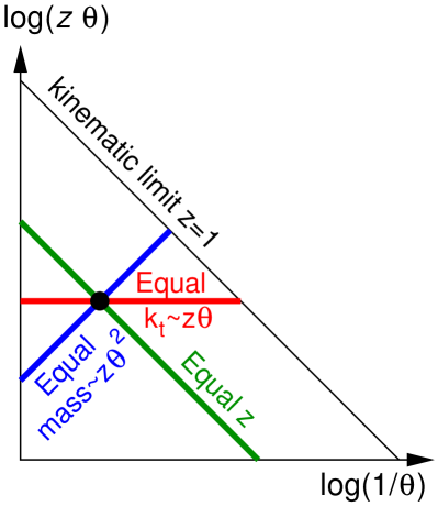
In the soft-and-collinear approximation, sufficient for the following discussion, each emission comes with a weight

$$d^{2}\omega=\frac{2\alpha_{s}(k_{t})C_{R}}{\pi}\,d\log(1/\theta)\,d\log(k_{t})\,,$$ (3)

with $C_{R}$ the colour factor of the parton initiating the jet, i.e. $C_{F}=4/3$ or $C_{A}=3$ respectively for quark and gluon jets. The strong coupling constant, $\alpha_{s}$, is evaluated at a scale equal to the transverse momentum of the emission relative to its emitter. Apart from running-coupling effects and subleading corrections in the hard-collinear and soft-large-angle regions, this weight is uniform over the Lund plane.

In the leading logarithmic approximation, the radiation in a jet is a superposition of independent and strongly-ordered (primary) emissions in that plane, as well as secondary emissions emitted from the primary emissions and which can be represented as extra Lund triangles (leaves) originating from each of the primary emissions, tertiary emissions emitted from secondary ones, etc… Leaves will be discussed in more detail below.

Figure 2: Lund diagram representation for the phasespace regions relevant to the full jet mass (left) and the mMDT mass (right). The solid black point corresponds to the emission dominating the jet mass and can be anywhere along the solid red line. It gives the prefactor in the jet mass distribution. The shaded red area corresponds to the vetoed region yielding the Sudakov exponent.

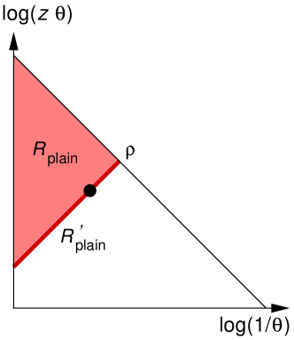
To illustrate how one can use this pictorial representation to discuss physics processes, let us consider the case of the (full) jet mass distribution $m^{2}\!/\sigma\>d\sigma/dm^{2}$. The corresponding Lund diagram is represented in the left panel of Fig. 2. One first needs an emission that provides the dominant contribution to the mass of the jet, i.e. an emission such that $m^{2}=z\theta^{2}p_{t}^{2}$ or such that $z\theta^{2}=\rho=(m/p_{t}R)^{2}$, where we have conveniently normalised the angles in units of the jet radius $R$ and introduced the dimensionless (squared) mass $\rho$ instead of $m^{2}$. For simplicity, we shall assume a jet radius of $R=1$ from now on. The integrated weight for emissions that generate a (normalised) jet mass equal to $\rho$ is

$$R_{\text{full}}^{\prime}(\rho)=\int d^{2}\omega\,\rho\delta(z\theta^{2}-\rho)\overset{{\text{f.c.}}}{=}\frac{\alpha_{s}C_{R}}{\pi}\log(1/\rho),$$ (4)

where for the last equality we have illustrated the structure of the answer in a fixed coupling approximation, as indicated by the superscript “f.c.”. Modulo corrections induced by the running of the strong coupling, the logarithmic behaviour basically comes from the integration over the solid line of equal mass in the Lund representation.

We also need to impose that no emissions occur at larger mass. This induces a Sudakov suppression $\exp[-R_{\text{full}}(\rho)]$ where

$$R_{\text{full}}(\rho)=\int d^{2}\omega\,\Theta(z\theta^{2}>\rho)\overset{{\text{f.c.}}}{=}\frac{\alpha_{s}C_{R}}{2\pi}\log^{2}(1/\rho).$$ (5)

The double-logarithmic behaviour corresponds to the shaded area in the Lund diagram. Note that $R_{\text{full}}^{\prime}(\rho)$ defined in Eq. (4) is the derivative of $R_{\text{full}}(\rho)$ with respect to $\log(1/\rho)$.

In the end, the leading-logarithmic (LL) result for the cross-section can be written as

$$\left.\frac{\rho}{\sigma}\frac{d\sigma}{d\rho}\right|_{\text{full}}=R_{\text{full}}^{\prime}(\rho)\,e^{-R_{\text{full}}(\rho)}.$$ (6)

This expression has a simple graphical representation: a prefactor corresponding to the emission setting the mass, the solid line in the Lund diagram, and a Sudakov suppression for larger masses, the shaded area in the Lund diagram.

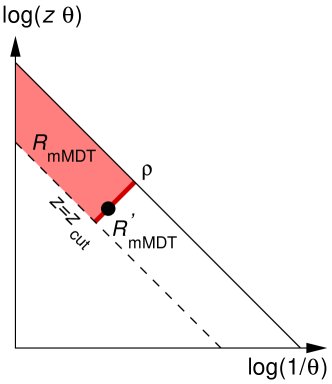
Let us now consider the jet mass distribution after the application of the mMDT. This is represented in the right panel of Fig. 2. In this case Dasgupta:2013ihk , emissions with $z<z_{\text{cut}}$ are discarded by the mMDT recursive procedure, so that both the prefactor $R_{\text{mMDT}}^{\prime}$ for having an emission setting the jet mass and the Sudakov exponent $R_{\text{mMDT}}$ are restricted to $z>z_{\text{cut}}$ and we have (assuming $\rho\ll z_{\text{cut}}\ll 1$),

$$\left.\frac{\rho}{\sigma}\frac{d\sigma}{d\rho}\right|_{\text{mMDT}} =R_{\text{mMDT}}^{\prime}(\rho)\,e^{-R_{\text{mMDT}}(\rho)},$$ (7a)

$$R_{\text{mMDT}}^{\prime}(\rho) =\int d^{2}\omega\,\rho\delta(z\theta^{2}-\rho)\Theta(z>z_{\text{cut}})\overset{{\text{f.c.}}}{=}\frac{\alpha_{s}C_{R}}{\pi}\log(1/z_{\text{cut}}),$$ (7b)

$$R_{\text{mMDT}}(\rho) =\int d^{2}\omega\,\Theta(z\theta^{2}>\rho)\Theta(z>z_{\text{cut}})\overset{{\text{f.c.}}}{=}\frac{\alpha_{s}C_{R}}{\pi}[\log(\rho)\log(z_{\text{cut}})-\frac{1}{2}\log^{2}(z_{\text{cut}})].$$ (7c)

Compared to the full mass result, Eq. (6), the prefactor is smaller but the Sudakov suppression is also less important. In practice, we will therefore have a suppression of the QCD background at intermediate masses but an increase at very small masses. More generally, we see that in order to have a large suppression of the QCD background, we want a method that keeps the prefactor small but gives a large Sudakov suppression. This will be a key element of our dichroic approach.

Next, we consider the signal (electroweak boson) jets in the context of Lund diagrams. For, say, a $W$ boson, the original splitting, $W\to q\bar{q}$ occurs on a line of constant mass $m=m_{W}$ and, since the corresponding splitting function does not have a $1/z$ divergence at small $z$, this splitting will be concentrated close to the large-$z$ end of that constant-mass line, with the small-$z$ tail exponentially suppressed (in our logarithmic choice of axes). As a direct consequence, no emissions are possible at larger mass and there will not be any Sudakov factor for that region. For simplicity in our discussion below, we will assume a constant splitting function in $z$, which would be the case e.g. for a Higgs boson or an unpolarised $W$ boson. For an mMDT $z_{\text{cut}}$ condition, this yields a signal efficiency of $1-2z_{\text{cut}}$. Subsequent emissions from the original $q\bar{q}$ pair will happen as if they were secondary emissions from these two quarks, i.e. essentially in two separate Lund planes each of them restricted to angles smaller than the separation $\theta_{q\bar{q}}$ between the two quarks, because of angular ordering. One of those Lund planes (that for the softer of the $q\bar{q}$ pair) will be represented as a leaf, cf. Fig. 3.

Now that we have discussed how mass distribution and radiation constraints are represented in terms of Lund diagrams, we will use Lund diagrams to discuss more complex substructure methods, leaving corresponding analytic expressions to section 5.

2.3 Radiation constraints ($N$-subjettiness)

Let us now examine how a cut on $N$-subjettiness on the full jet affects the pattern of allowed radiation. Our discussion will be in a context where the full jet has a specified mass, denoted through $\rho$. The constraints imposed by a cut on the $N$-subjettiness ratio $\tau_{21}$ can then again be presented quite straightforwardly in terms of Lund diagrams, at least in the small $\tau_{21}$ limit, which is what we will consider in our discussion.

Figure 3: Lund diagram for QCD background jets (left) and signal jets (right) corresponding to the requirement of a given full jet mass with a cut on the $N$-subjettiness ratio $\tau_{21}$. The red shaded region (present only in the background case) corresponds to the Sudakov vetoed region for the mass, as in Fig. 2, together with the prefactor for having an emission on the solid red line. The blue shaded region corresponds to the additional veto coming from the cut on $N$-subjettiness. The dashed/dotted red line for the signal case represents the fact that, for signal jets, small-$z$ configurations are exponentially suppressed. The region that emerges from the plane is referred to as a “leaf” and in the left-hand diagram represents secondary emissions from emission $1$, while in the right-hand diagram it represents emissions from the softer of the two prongs of the decay.

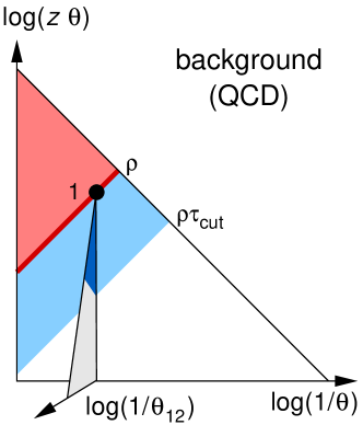
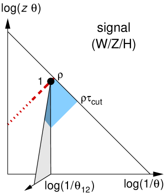
Say that we have a first emission with an angle $\theta_{1}$ and momentum fraction $z_{1}$ that dominates the jet mass, $\rho=z_{1}\theta_{1}^{2}$. It can be shown Dasgupta:2015lxh that, in our leading-logarithmic approximation, $\tau_{N}$ (with $\beta_{\tau}=2$) will be dominated by the $N^{\text{th}}$ largest $z\theta^{2}$. We therefore have $\tau_{1}\equiv\rho$ and imposing a cut $\tau_{21}<\tau_{\text{cut}}$ is equivalent to vetoing emissions down to a “mass-like scale” $z\theta^{2}=\rho\tau_{\text{cut}}$, for both primary and secondary emissions. This is represented in Fig. 3 for QCD and signal jets, where the extra constraint on $N$-subjettiness corresponds to an extra Sudakov factor represented by the blue shaded region. In the background case, the leaf that emerges from the plane corresponds to a region of secondary emissions, while in the signal it corresponds to the region of emissions from the softer of the $q\bar{q}$ pair. Assuming a background mainly consisting of quark jets, the main parts of the plane in the two figures are both associated with a $C_{F}$ colour factor, while the leaf in the background case is associated with a $C_{A}$ colour factor, in contrast with the $C_{F}$ factor for the signal, and correspondingly represented with a darker shade of blue.

We see that we now have a Sudakov suppression for both the signal and the QCD background. Since the vetoed area is larger for the background than for the signal, the former is more suppressed than the latter, implying a gain in discriminating power. Furthermore, since, for a given $\tau_{\text{cut}}$, the vetoed area increases when $\rho$ gets smaller, the discriminating power will also be larger for more boosted jets.

3 Dichroic subjettiness ratios

3.1 Combining mMDT/SD with $N$-subjettiness

We can now present the main proposal of this paper concerning the dichroic combination of a tagger with a radiation constraint. The discussion below assumes that we use SoftDrop or the modified MassDrop tagger as our tagger and a cut on $\tau_{21}$ as a radiation constraint, but we believe that the core argument can also be applied to other shapes, for example to energy correlation functions Larkoski:2013eya ; Larkoski:2014gra ; Moult:2016cvt .

Let us consider a high-$p_{t}$ large-radius ($R\simeq 1$) jet on which we have applied an mMDT (or SD) tagger. The original large-radius jet will be called the full jet. The part of the jet that remains after the mMDT/SD tagging procedure will be called the tagged jet, and has an angular size comparable to the angle between the two hard prongs identified by the tagger. The $N$-subjettiness variables $\tau_{1}$ and $\tau_{2}$ can be evaluated either on the full or the tagged jet and there are three combinations of interest:

$$\tau_{21}^{\text{tagged}} \equiv\frac{\tau_{2}^{\text{tagged}}}{\tau_{1}^{\text{tagged}}},$$ (8a)

$$\tau_{21}^{\text{full}} \equiv\frac{\tau_{2}^{\text{full}}}{\tau_{1}^{\text{full}}},$$ (8b)

$$\tau_{21}^{\text{dichroic}} \equiv\frac{\tau_{2}^{\text{full}}}{\tau_{1}^{\text{tagged}}}.$$ (8c)

The first two options are currently widely used in the literature (see e.g. Behr:2015oqq ; Aad:2015typ ; Khachatryan:2016cfa ; Dolen:2016kst ; Khachatryan:2016mdm for recent examples). The third, “dichroic”, option is a new combination, and is the subject of this paper.

To understand how these different variants work, we will take two approaches. First we will consider what values of $\tau_{21}$ arise for different kinematic configurations involving three particles in the jet, i.e. two emissions in the case of QCD jets, and the original two prongs plus one additional emission in the case of signal jets. Then we will use this information to understand how a cut on $\tau_{21}$ constrains the radiation inside the jet.

During this discussion it will be useful to keep in mind the core difference between signal and background jets. In the case of the background jets, the whole Lund plane and the leaf can contain emissions, as shown in Fig. 3(left). In the case of signal jets, emissions are mostly limited to the region shown in blue in Fig. 3(right), i.e. at angles smaller than the decay opening angle and transverse momenta smaller than the mass. The leaves in the two cases have different colour factors, however we will neglect this aspect in our discussion. Rather we will concentrate on the differences that arise at large angle, i.e. from the different coherent radiation patterns of coloured versus net colour-neutral objects.

	Case 1		Case 2		Case 3
	$z_{c}\theta_{c}^{2}\ll z_{b}\theta_{b}^{2}\ll z_{a}\theta_{a}^{2}$		$z_{b}\theta_{b}^{2}\ll z_{c}\theta_{c}^{2}\ll z_{a}\theta_{a}^{2}$		$z_{b}\theta_{b}^{2}\ll z_{a}\theta_{a}^{2}\ll z_{c}\theta_{c}^{2}$
	bkg	sig	bkg	sig	bkg	sig
$\tau_{21}^{\text{tagged}}$	b/a	b/a	b/a	b/a	b/a	b/a
$\tau_{21}^{\text{full}}$	b/a	b/a	c/a	b/a	a/c	b/a
$\tau_{21}^{\text{dichroic}}$	b/a	b/a	c/a	b/a	a/a	b/a

Figure 4: Schematic representation of three possible kinematic configurations for the combination of $\tau_{21}$ with mMDT/SD (shown specifically for mMDT or SD with $\beta=0$). In each Lund diagram, emission “a” corresponds to the emission that dominates the mMDT/SD jet mass. This defines three regions: region A (red) is vetoed by mMDT, region B (blue) contains the constituents of the mMDT/SD jet and region C (blue) is the difference between the mMDT/SD jet and the full jet. Emissions “b” and “c” are respectively in regions B and C, and the three plots correspond to three different orderings of $z_{c}\theta_{c}^{2}$ compared to $z_{a}\theta_{a}^{2}$ and $z_{b}\theta_{b}^{2}$. The table below the plots shows the corresponding value of $\tau_{21}$ for both the QCD background (where all three regions have to be included) and the signal (where only regions A and B are present). For simplicity, “b/a” stands for $(z_{b}\theta_{b}^{2})/(z_{a}\theta_{a}^{2})$, and so forth.

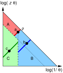
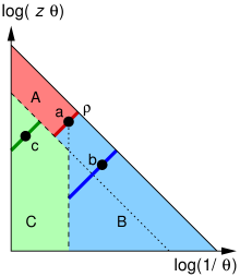
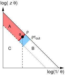
We consider the situation where, after the tagger has been applied, the tagged jet mass is dominated by emission “a”, i.e. $\rho\approx z_{a}\theta_{a}^{2}$ (in the case of the signal jet this is the softer of the two prongs). The Lund-plane phasespace can then be separated into 3 regions depicted in Fig. 4. Region A (in red) is the region that is constrained to be free of radiation by the fact that the tagger has triggered on emission a. This corresponds to the region where both $z\theta^{2}>z_{a}\theta_{a}^{2}$ and Eq. (1) are satisfied. It is responsible for the Sudakov exponent associated with the tagger, cf. Eq. (7).

Of the remaining phasespace, region B (blue) corresponds to emissions that are contained inside the tagged jet. It is populated in both signal and background cases. It contains not only emissions that satisfy the mMDT/SD condition ($z>z_{\text{cut}}$ in the case of mMDT), but also emissions with $z\theta^{2}<z_{a}\theta^{2}_{a}$ and $\theta<\theta_{a}$, due to the Cambridge/Aachen declustering used by mMDT/SD. Region C (green) corresponds to emissions that are in the original full jet, but not in the tagged jet. It is uniformly populated in the background case, while in the signal case it is mostly empty of radiation, except at the left-hand edge (initial-state radiation) and the right-hand edge (leakage of radiation from the colour-singlet $q\bar{q}$ decay). The emission with the largest $z\theta^{2}$ in each of regions B and C will respectively be labelled $b$ and $c$ and we will assume strong ordering between emissions, as in section 2.

There are three kinematic cases to consider for the relative $z\theta^{2}$ ordering of emissions $a$, $b$ and $c$, cf. Fig. 4. In each case, Fig. 4 gives the result for each of the $\tau_{21}$ variants, for both background and signal. The signal case simply assumes that there are no emissions in region C, which is appropriate in a double-logarithmic approximation. The results are expressed as a shorthand, $i/j\equiv z_{i}\theta_{i}^{2}/z_{j}\theta_{j}^{2}$.

The case of the signal is particularly simple: since $z_{b}\theta_{b}^{2}<z_{a}\theta_{a}^{2}$ and there is nothing in region C, all variants give $\tau_{21}=z_{b}\theta_{b}^{2}/z_{a}\theta_{a}^{2}$. Given that the signal result is always the same, the performance of the signal/background discrimination will be best for the method that gives the largest background $\tau_{21}$ result (recall that one enhances signal relative to background by requiring $\tau_{21}<\tau_{\text{cut}}$).

Let us examine the background separately for each of the three kinematic cases shown in Fig. 4:

1. For $z_{a}\theta_{a}^{2}\gg z_{b}\theta_{b}^{2}\gg z_{c}\theta_{c}^{2}$, all three $\tau_{21}$ variants give the same result as for the signal, $z_{b}\theta_{b}^{2}/z_{a}\theta_{a}^{2}$.

2. For $z_{a}^{2}\theta_{a}^{2}\gg z_{c}^{2}\theta_{c}^{2}\gg z_{b}^{2}\theta_{b}^{2}$, $\tau_{21}^{\text{tagged}}$ is still still given by $z_{b}\theta_{b}^{2}/z_{a}\theta_{a}^{2}$, but $\tau_{21}^{\text{full}}$ and $\tau_{21}^{\text{dichroic}}$ now both take the larger value of $z_{c}\theta_{c}^{2}/z_{a}\theta_{a}^{2}$. They should therefore perform better in this case.

3. Finally, for $z_{c}^{2}\theta_{c}^{2}\gg z_{a}^{2}\theta_{a}^{2}\gg z_{b}^{2}\theta_{b}^{2}$, $\tau_{21}^{\text{tagged}}$ is again given by $z_{b}\theta_{b}^{2}/z_{a}\theta_{a}^{2}$; $\tau_{21}^{\text{full}}$ is given by $z_{a}\theta_{a}^{2}/z_{c}\theta_{c}^{2}$, since $\tau_{1}$ is dominated by emission $c$, while $\tau_{2}$ is dominated by emission $a$. Depending on the exact configuration, $\tau_{21}^{\text{full}}$ may be larger or smaller than $z_{b}\theta_{b}^{2}/z_{a}\theta_{a}^{2}$ and so may or may not be advantageous. $\tau_{21}^{\text{dichroic}}$ has a value of $z_{a}\theta_{a}^{2}/z_{a}\theta_{a}^{2}=1$, which is always larger than the signal and larger than the other two variants.

Overall therefore, $\tau_{21}^{\text{dichroic}}$ is expected to be the best of the three variants.

(i)

(ii)

(iii)

Figure 5: Regions where real emissions are vetoed when combining a mMDT/SD tagger with a cut on $\tau_{21}$. See text for details.

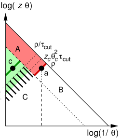
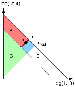
Alternatively, we can also see the benefit of the dichroic combination by examining directly how emissions are constrained when one applies a given cut on the $\tau_{21}$ ratio, similarly to the discussion in Section 2.3. We have represented the Lund diagrams relevant for our discussion in Fig. 5, where we have used the same regions A, B and C as in the above discussion.

We start by considering a jet for which we already have applied the mMDT/SD procedure, resulting in a (mMDT/SD) mass $\rho$ dominated by emission “a”. This automatically comes with a mMDT/SD prefactor and Sudakov suppression represented by the solid red line and shaded light red area (region A) in Fig. 5, guaranteeing that there are no emissions at larger mass kept by the mMDT/SD.

For $\tau_{21}^{\text{tagged}}$, emissions in region B are vetoed down to a mass scale $\rho\tau_{\text{cut}}$ while emissions in region C, i.e. outside the mMDT/SD tagged jet, are left unconstrained. This results in the (additional) Sudakov suppression given by the blue area (region B) in Fig. 5LABEL:sub@fig:combination-3lund-i.

The situation for $\tau_{21}^{\text{full}}$ is a bit more involved and we have three cases to consider. The first case is when there is (at least) one emission in region C with $z\theta^{2}>z_{a}\theta_{a}^{2}/\tau_{\text{cut}}\equiv\rho/\tau_{\text{cut}}$ and is represented in Fig. 5LABEL:sub@fig:combination-3lund-ii. Let us then call emission “c” the emission in region C with the largest $z\theta^{2}$, which thus comes with a Sudakov suppression imposing that there are no other emissions in region C with $z\theta^{2}>z_{c}\theta_{c}^{2}$. Emission “c” will dominate $\tau_{1}$ so that the cut on $\tau_{21}$ will come with an extra suppression factor in region C extending from $z_{c}\theta_{c}^{2}$ down to $z\theta^{2}=z_{c}\theta_{c}^{2}\tau_{\text{cut}}$. Consequently, all emissions down to $z_{c}\theta_{c}^{2}\tau_{\text{cut}}$ are vetoed as depicted in Fig. 5LABEL:sub@fig:combination-3lund-ii. The second case is when the emission in region C with the largest $z\theta^{2}$ satisfies $z_{a}\theta_{a}^{2}\equiv\rho<z_{c}\theta_{c}^{2}<\rho/\tau_{\text{cut}}$. This region, represented by the hatched area in Fig. 5LABEL:sub@fig:combination-3lund-ii, is entirely forbidden because it would give a value of $\tau_{21}\geq z_{a}\theta_{a}^{2}/z_{c}\theta_{c}^{2}$ which is always larger than $\tau_{\text{cut}}$. The third case is when there are no emissions in region C with $z\theta^{2}>\rho$. This directly comes with a Sudakov suppression in region C vetoing emission down to $z\theta^{2}=\rho$. In this case, $\tau_{1}$ is dominated by emission “a” and the constraint on $\tau_{21}$ further vetoes emissions with $\rho\tau_{\text{cut}}<z\theta^{2}<\rho$ in both regions B and C. These two vetoes combine to vetoing all emission down to $\rho\tau_{\text{cut}}$ as represented in Fig. 5LABEL:sub@fig:combination-3lund-iii.

If instead we use our new $\tau_{21}^{\text{dichroic}}$ variable, we are always in the situation of Fig. 5LABEL:sub@fig:combination-3lund-iii, where we veto all emissions down to a mass scale $\rho\tau_{\text{cut}}$ in both regions B and C. This new version therefore comes with the strongest Sudakov suppression, i.e. of the three $\tau_{21}$ variables it is the one that, for background jets, is least likely to have a small $\tau_{21}$ value. Given that the three $\tau_{21}$ variants behave similarly to each other for signal, the signal-to-background discrimination should be improved for the dichroic variant.

With our dichroic method, we actually recover the same overall Sudakov suppression as the one we had when measuring the full jet mass and cutting on the full $N$-subjettiness (see Section 2.3 and Fig. 3(left)). The gain of our new method (8c) compared to this full $N$-subjettiness case comes from the fact that the prefactor associated with the jet mass is now subject to the constraint imposed by the tagger. If we take for example the case of the mMDT, this prefactor would be largely suppressed for the background — going from $\sim\alpha_{s}\log(1/\rho)$ for full $N$-subjettiness to $\sim\alpha_{s}\log(1/z_{\text{cut}})$ for the dichroic method — while the signal would only be suppressed by a much smaller factor $\sim 1-2z_{\text{cut}}$. Additionally, measuring the tagged jet mass instead of the full jet mass significantly reduces ISR and non-perturbative effects which would otherwise affect the resolution of the signal mass peak (see also Dasgupta:2015yua ; ourYsplitter ).

Finally, we note that the gain in performance is expected to increase for larger boosts due to region C getting bigger (double-logarithmically in $\rho$).

3.2 Dichroic subjettiness with SoftDrop (pre-)grooming

Since $\tau_{21}^{\text{dichroic}}$ uses $\tau_{2}$ computed on the full jet, including all the soft radiation at large angles, we can expect this observable to be quite sensitive to poorly-controlled non-perturbative effects — hadronisation and the Underlying Event — and to pileup.

The standard strategy to mitigate these effects is to kill two birds with one stone and to use mMDT (or SD) both as a two-prong tagger and as a groomer, and impose the $\tau_{21}$ constraint on the result. This is equivalent to the $\tau_{21}^{\text{tagged}}$ variant discussed (Fig. 5(a)), with the drawback and loss of performance described in the previous Section.

We show here how we can achieve a background rejection that is larger than for $\tau_{21}^{\text{tagged}}$ and more robust with respect to non-perturbative effects than $\tau_{21}^{\text{dichroic}}$. Conceptually, the idea is that the tagger and groomer achieve two different tasks: the tagger selects a two-prong structure in the jet, imposing a rather hard constraint on the soft radiation in order to do so, leading to a small $R^{\prime}$ prefactor for the jet mass. This is not quite what we want from a groomer, which should get rid of the soft-and-large-angle radiation while retaining enough of the jet substructure to have some discriminating power when using radiation constraints.

Figure 6: Phasespace constraints on QCD jets obtained from our new combination including grooming: we first groom the jet, e.g. with SoftDrop (SD). We then compute both the jet mass and $\tau_{1}$ on the tagged jet (here using the mMDT), yielding the solid red line prefactor and the shaded red region (A) for the Sudakov exponent. We then impose a cut on the $\tau_{21}$ ratio with $\tau_{2}$ computed on the SD jet, leading to the extra shaded blue and green regions (B and C) for the Sudakov exponent.

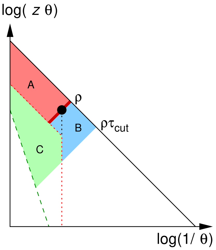
This suggests the following picture: we first apply a “gentle” grooming procedure to the jet, like a SoftDrop procedure with a positive value of $\beta$. This is meant to clean the jet of the unwanted soft junk while retaining as much as possible the information about the perturbative radiation in the jet. We can then carry on with the dichroic method presented in the previous Section, i.e. use a more aggressive tagger, like mMDT, to compute the jet mass and $\tau_{1}$ and compute $\tau_{2}$ on the SD (pre-)groomed jet:

$$\tau_{21,\text{groomed}}^{\text{dichroic}}=\frac{\tau_{2}(\text{SD jet})}{\tau_{1}(\text{mMDT jet})}.$$ (9)

This is depicted in Fig. 6, where regions A and B are the same as in the previous Section, but now region C indicates the region where emissions are kept by the groomer but rejected by the tagger. Similarly, we can introduce

$$\tau_{21,\text{groomed}}^{\text{full}}=\frac{\tau_{2}(\text{SD jet})}{\tau_{1}(\text{SD jet})}.$$ (10)

Note that we will always choose our mMDT-tagging and SD-grooming parameters such that the tagged jet is the same whether tagging is performed before or after grooming. For mMDT-tagging with parameter $z_{\text{cut}}$ and SD-grooming with parameters $\zeta_{\text{cut}}$ and $\beta$, this implies $\zeta_{\text{cut}}\leq z_{\text{cut}}$ and $\beta\geq 0$.

Using the same arguments as in Section 3.1, we can show straightforwardly that this method will have a larger rejection than with the other two variants where one would be computing the jet mass on the mMDT-tagged jet and the $\tau_{21}$ ratio either on the mMDT-tagged jet, $\tau_{21,\text{groomed}}^{\text{tagged}}\equiv\tau_{21}^{\text{tagged}}$, or on the SD-groomed jet, $\tau_{21,\text{groomed}}^{\text{full}}$, owing to a larger Sudakov suppression of the background, for a similar signal efficiency.

Compared to the other possible situation where both the jet mass and the $\tau_{21}$ ratio are computed on the SD-groomed jet, the dichroic variant would have a smaller $R^{\prime}$ prefactor, associated with mMDT instead of SD. This again leads to a larger background rejection.

Because of the initial grooming step, the groomed dichroic subjettiness ration is expected to be less discriminating than the ungroomed version introduced in Section 3.1. Indeed, the associated Sudakov exponent is smaller since we have amputated part of the soft-large-angle region. One should however expect that this groomed variant will be less sensitive to non-perturbative effects. Overall, there is therefore a trade-off between effectiveness, in terms of achieving the largest suppression of the QCD background for a given signal efficiency, and perturbative robustness, in terms of limiting the sensitivity to poorly-controlled non-perturbative effects.

4 Performance in Monte-Carlo simulations

Let us now investigate the effectiveness and robustness of dichroic subjettiness ratios in Monte-Carlo simulations, using Pythia 8.186 pythia , at a centre-of-mass energy of $\sqrt{s}=13$ TeV. Our signal sample consists of $WW$ events, while for the background we use dijet events. Jets are reconstructed with the anti-$k_{t}$ Cacciari:2008gp algorithm with $R=1$ and in determining signal and background efficiencies we keep all jets above a given $p_{t}$ cut. We use the modified MassDrop tagger with $z_{\text{cut}}=0.1$ for the 2-prong tagging and vary the cut on the $\tau_{21}$ ratio. Whenever a SoftDrop (SD) grooming procedure is included, we use $\zeta_{\text{cut}}=0.05$ and $\beta=2$ as illustrative parameter choices (recall that the SoftDrop condition is imposed as $z>\zeta_{\text{cut}}(\theta_{12}/R)^{\beta}$ instead of Eq. (1), i.e. we use separate symbols $z_{\text{cut}}$ and $\zeta_{\text{cut}}$ respectively for the parameters of mMDT and SD). Jet reconstruction and manipulation are performed with FastJet 3.2.0 Cacciari:2005hq ; Cacciari:2011ma and fjcontrib 1.024 fjcontrib .

4.1 $N$-subjettiness and mass distributions with various $\tau_{21}$ ratios ($\beta_{\tau}=2$)

Figure 7: $\tau_{21}$ distributions for jets in dijet (solid lines) and $WW$ (dashed lines) events again imposing $p_{t}>2$ TeV and including SoftDrop grooming. Different colours correspond to different combinations of jets used for the computation of the jet mass, $\tau_{1}$ and $\tau_{2}$ as indicated in the legend, our new dichroic combination being plotted in black. We have selected jets with a mass is between 60 and 100 GeV. The cross-section used for normalisation, $\sigma$, is defined after the jet $p_{t}$ and mass cut, so that all curves integrate to one.

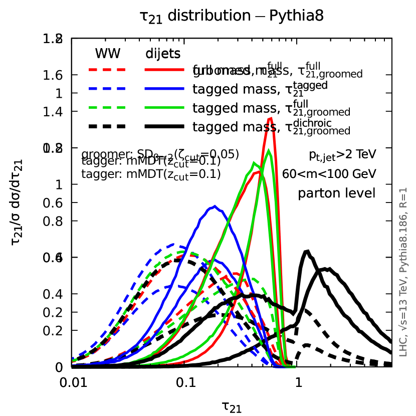
We start by examining the $\tau_{21}$ distribution. This is plotted in Fig. 7 for both QCD jets (solid lines) in dijet events and $W$ jets (dashed lines) in $WW$ events. We select jets above 2 TeV and always apply SoftDrop grooming. In practice, we use parton-level events, and impose a cut on the reconstructed jet mass (SD-groomed or mMDT-tagged) $60<m<100$ GeV. We consider four cases: the $\tau_{21,\text{groomed}}^{\text{full}}$ distribution when we cut on the SD-groomed mass and the $\tau_{21}^{\text{tagged}}$, $\tau_{21,\text{groomed}}^{\text{full}}$ and $\tau_{21,\text{groomed}}^{\text{dichroic}}$ distributions when we cut on the mMDT-tagged mass. As expected, the distributions for signal ($W$) jets are peaked at smaller values of $\tau_{21}$ than the corresponding distribution for background (QCD) jets. Fig. 7 shows that all the signal distributions, and in particular the three options where one measures the mMDT-tagged jet mass, are very similar. This is in agreement with our discussion in the previous Section. Comparatively the background distributions look rather different. The case where everything is computed from the mMDT-tagged jet (the solid blue curve) peaks at smaller values of $\tau_{21}$ as expected from its smaller Sudakov suppression, related to the fact that this combination puts no constraints on large-angle emissions (region C in the previous Section). Furthermore, the dichroic combination, the solid black curve in Fig. 7, is expected to have the largest suppression and is indeed peaked at larger $\tau_{21}$ values, translating into a larger discrimination against signal jets.

Note that the $\tau_{21}$ distribution for the dichroic combination also shows a peak for $\tau_{12}>1$ that we have not discussed in our earlier argumentation. This comes from events with multiple emissions in region C and will be discussed briefly in our analytic calculations in Section 5.

Results for the mass distribution obtained for background (QCD dijets) jets at parton level (without UE) are presented in Fig. 8. As in Fig. 7, SoftDrop grooming has always been applied prior to any additional tagging or $N$-subjettiness cut. Again, we can identify most of the features discussed in section 3. First of all, if we compare the mMDT-tagged mass (dashed blue curve) to the SD-groomed jet mass (dashed red curve) we see that the latter is smaller than the former at small masses, owing to the larger Sudakov factor $R_{\text{SD}}>R_{\text{mMDT}}$, but larger at intermediate masses, due to the larger prefactor $R_{\text{SD}}^{\prime}>R_{\text{mMDT}}^{\prime}$.

Figure 8: Mass distribution for QCD jets with $p_{t}>2$ TeV (anti-$k_{t}$, $R=1$) at parton level, including SoftDrop grooming. The dashed lines, in red for the SD-groomed jet and in blue for the mMDT-tagged jet, are the mass distributions with no constraint on $N$-subjettiness. The solid lines have an additional cut $\tau_{21}<0.3$ with different combinations of jets used for the computation of the jet mass, $\tau_{1}$ and $\tau_{2}$ as indicated in the legend, our dichroic combination being plotted using a solid black line. The cross section used for normalisation, $\sigma$ is that for jets above the $p_{t}$ cut.

Then, we can consider the effect of the additional constraint on the $\tau_{21}$ ratio, taken here as $\tau_{21}<0.3$ for illustrative purpose. If we compute $\tau_{21}$ on the same jet as for the mass ($\tau_{21,\text{groomed}}^{\text{full}}$ in solid red and $\tau_{21}^{\text{tagged}}$ in solid blue for the SD-groomed and mMDT-tagged jets respectively), we see that the cut reduces the background, that the reduction increases for smaller masses and that the reduction is larger for the SD-groomed jet than for the mMDT-tagged jet. This last point is a reflection of the fact, that the Sudakov suppression associated with the $N$-subjettiness cut is larger when both the mass and $\tau_{21}$ are computed on the SD-groomed jet (Fig. 3(left)) than when both the mass and $\tau_{21}$ are computed on the mMDT-tagged jet (Fig. 5(left)). Then, when measuring the mMDT-tagged jet mass, one sees that computing $\tau_{21}$ on the SD-groomed jet ($\tau_{21,\text{groomed}}^{\text{full}}$, the solid green curve in Fig. 8) shows a larger suppression than computing $\tau_{21}$ on the mMDT-tagged jet, although the difference is reduced at very small masses. Finally, if we consider our new, dichroic case, Eq. (9) ($\tau_{21,\text{groomed}}^{\text{dichroic}}$, the solid black curve), we see a larger suppression than in all other cases, as expected from our earlier arguments.

4.2 Signal v. background discrimination and other performance measures

Figure 9: ROC curves for various $\tau_{21}$ combinations, i.e. background versus signal efficiency, at parton level. The left plot is obtained starting from the full jet, while for the right plot, a SoftDrop grooming step has been applied. The ROC curves are obtained by varying the cut on the $\tau_{21}$ ratio. In all cases, we considered anti-$k_{t}$($R=1$) jets with $p_{t}>2$ TeV.

Figure 10: Same as figure as 9, now for hadron level (including the Underlying Event).

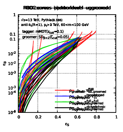
To further test the performance of our new method, we have also studied ROC (receiver operating characteristic) curves, shown in Fig. 9 for parton-level simulations and in Fig. 10 for hadron-level events including hadronisation and the Underlying Event. In all cases, we impose the constraint that the mass is between 60 and 100 GeV. Efficiencies are given relative to the inclusive cross-section for having jets above our $p_{t}$ cut.

Let us first discuss the result of parton-level simulations, Fig. 9, where the dichroic ratio is again represented by the black curves. Without grooming (the left-hand plot in the figure), our method shows a substantial improvement compared to all other combinations considered, outperforming them by almost 30% in background rejection at a signal efficiency of 50% and by more than a factor of 2 at a signal efficiency of 40%. After SoftDrop grooming (right-hand plot), the dichroic method, i.e. computing the jet mass and $\tau_{1}$ on the mMDT-tagged jet and $\tau_{2}$ on the SD-groomed jet, still shows an improvement, albeit less impressive than what is observed using the full jet to compute $\tau_{2}$.

If instead we consider the results at hadron level, including both the perturbative parton shower as well as non-perturbative effects, Fig. 10, we see that the dichroic subjettiness ratio still does a better job than the other variants but the gain is smaller. For example, measuring the mMDT-tagged mass with a cut on the groomed dichroic ratio, $\tau_{21,\text{groomed}}^{\text{dichroic}}$, the optimal choice in Fig. 10, is only slightly better than the next best choice where one measures the SD-groomed mass and imposes a constraint on $\tau_{21,\text{groomed}}^{\text{full}}$. This is because in going from parton to hadron level, the $\rho_{\text{groomed}}$–$\tau_{21,\text{groomed}}^{\text{full}}$ curve has moved down more than the $\rho_{\text{tagged}}$–$\tau_{21,\text{groomed}}^{\text{dichroic}}$ curve, i.e. the former is getting a significantly larger boost in its discriminating power from non-perturbative effects. This is potentially problematic, because one does not necessarily want signal-to-background discrimination power for a multi-TeV object to be substantially driven by the physics that takes place at a scale of $1\,\text{GeV}$, physics that cannot, with today’s techniques, be predicted from first principles. Additionally, phenomena happening on a scale of $1\,\text{GeV}$ are difficult to measure reliably.

It would be interesting to investigate non-perturbative effects in greater depth, both analytically, e.g. following the approach used in Dasgupta:2013ihk , or by studying their dependence across different Monte-Carlo generators and associated tunes. However, for the purpose of this article, we limit ourselves to using the results from Pythia 8. In evaluating the overall performance of different $\tau_{21}$ combinations we will consider both the signal significance and the size of non-perturbative effects. We will use the following alternative to ROC curves. For a given method and $p_{t}$ cut, we first determine the $\tau_{21}$ cut required to obtain a desired signal efficiency (at hadron level). For that value of the $\tau_{21}$ cut, we can compute the signal significance, defined as $\epsilon_{S}/\sqrt{\epsilon_{B}}$ (computed at hadron level) which is a measure of the discriminating power of the method; we then estimate non-perturbative effects as the ratio between the background efficiency at hadron level divided by the background efficiency at parton level, which is a measure of robustness against non-perturbative effects. We will show results for a range of different signal-efficiency choices and jet $p_{t}$ cuts.

Figure 11: Signal significance plotted versus the non-perturbative effects for the QCD background (defined as the ratio between the background “fake” tagging rate at hadron and parton level). Different curves correspond to different combinations indicated in the legend. For the solid curves, a SoftDrop ($\beta=2$ and $\zeta_{\text{cut}}=0.05$) grooming is applied, while no grooming is applied for the dashed curves. In the left-hand plot, we impose a 2 TeV $p_{t}$ cut on the initial jet. The symbols on each curve then correspond to a signal efficiency (computed at hadron level) ranging from 0.05 upwards in steps of 0.05, with the large symbol on each line corresponding to $\varepsilon_{S}=0.5$ and the efficiency at the right-hand extremity explicitly labelled. In the right-hand plot, the signal efficiency (computed at hadron level) is fixed to be 0.5 and the $p_{t}$ cut on the jet is varied between 500 GeV and 3 TeV (in steps of 500 GeV, labelled explicitly for the groomed dichroic ratio), with the large symbol on each line corresponding to a 3 TeV cut.

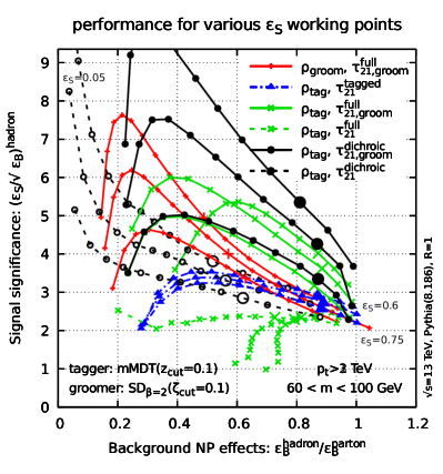
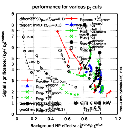
In Fig. 11, which highlights the key performance features of the dichroic method, we plot the signal significance versus the non-perturbative effects for different methods. In the left-hand panel, the curves correspond to a range of $\tau_{21}$ cuts for jets with $p_{t}>2\,\text{TeV}$. The points on the curves correspond to different signal efficiencies (starting from 0.05, in steps of 0.05, and with $\epsilon_{S}=0.5$ indicated by a bigger point). In the right-hand panel, the points on the curves correspond to different $p_{t}$ cuts, with the $\tau_{21}$ cut adjusted (as a function of $p_{t}$) so as to ensure a constant signal efficiency of $0.5$. To avoid the proliferation of curves, the result for the ungroomed $\rho_{\text{full}}$–$\tau_{21}^{\text{full}}$ is not shown since it is obvious from the ROC curves in Figs. 9 and 10(left) that it is extremely sensitive to non-perturbative effects.

In both plots, we see that the dichroic method comes with larger discriminating power with a relatively limited sensitivity to non-perturbative effects, provided one first applies a grooming step. Without the grooming step, one observes a much larger sensitivity to non-perturbative effects, as one might expect. It also appears that the performance gain increases when the boost, i.e. the jet $p_{t}$, increases. This was also expected from our arguments in Section 3. Finally, compared to the common setups in the literature, namely with modified MassDrop tagging with a cut on $\tau_{21}$ applied either on the mMDT ($\rho_{\text{tag}}$–$\tau_{21}^{\text{tagged}}$, the dot-dashed blue curve) or on the full jet ($\rho_{\text{tag}}$–$\tau_{21}^{\text{full}}$, the dashed green curve), our dichroic method with grooming (solid black) gives up to a factor of two improvement in signal significance, with comparable non-perturbative effects. Considering other combinations that have not been widely used experimentally, $\tau_{21,\text{groomed}}^{\text{full}}$ with either a groomed ($\rho_{\text{groom}}$, solid red) or a tagged ($\rho_{\text{tag}}$), solid green) jet mass both perform well, however $\tau_{21,\text{groomed}}^{\text{dichroic}}$ still remains the best, with an optimal significance that is about $25\%$ larger, and smaller non-perturbative corrections for any given signal significance.

Figure 12: Signal efficiency plotted as a function of the cut $\tau_{\text{cut}}$ on $\tau_{21}$ for all the combinations considered in Figs. 9 and 10. Solid curves correspond to hadron-level results while dashed curves are obtained at parton level. The left plot is obtained starting from the full jet, while for the right plot, a SoftDrop grooming has been applied.

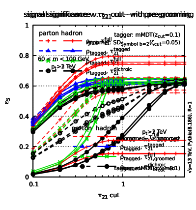
As a final check, we have studied the dependence of the signal efficiency on the $\tau_{21}$ cut, as shown in Fig. 12. Comparing the left and right-hand plots, it appears clearly that applying SoftDrop grooming helps to reduce non-perturbative effects which otherwise significantly lower the signal efficiency. It is also interesting to notice that without grooming, the signal efficiency obtained with our dichroic method (the dashed black curve on the left plot of Fig. 12) only reaches its plateau for cuts on $\tau_{21}$ larger than 1 already at parton level. This can likely be attributed to initial-state radiation in the jet at angles larger than the decay angle of the $W$ boson. These effects are strongly reduced by SoftDrop grooming (see also the discussion in Section 5).

In the end, a more complete study would include variations of the SD parameters and of the cuts on the mass. A brief investigation of the SD parameters shows that our choice of $\beta=2$ and $\zeta_{\text{cut}}=0.05$ seems a decent default, at least for the process and kinematic domain under study. However, in view of the good signal efficiency reached when computing both the jet mass and $\tau_{21}$ with SoftDrop, it might also be interesting to investigate our dichroic combination where we also use SoftDrop for the tagger instead of the mMDT. An extensive analytic study foreseen in a follow-up paper tau21-calculation would allow for a systematic study of these effects. Such an analytic understanding could also be of use in the context of building decorrelated taggers Dolen:2016kst .

4.3 Brief comparison with other tools

To complete our Monte Carlo studies, in Fig. 13 we compare the performance of $\tau_{21,\text{groomed}}^{\text{dichroic}}$ with various other tools: mMDT tagging alone, SoftDrop grooming alone ($\beta=2$ as above), and also the Y${}_{\text{m}}$ variant ourYsplitter of Y-splitter Butterworth:2002tt , combined either with SoftDrop (pre-)grooming or with trimming, as described in detail in Ref. ourYsplitter (see also Ref. Dasgupta:2015yua ). Whereas in the analogous Fig. 11, all curves involved the same signal efficiency, here this is no longer the case. Accordingly efficiencies are reported versus $p_{t}$ in table 1.

Figure 13: Signal significance and non-perturbative effects for background, for jet $p_{t}$ cuts ranging from $500\,\text{GeV}$ to $3\,\text{TeV}$ in steps of $500\,\text{GeV}$, as in Fig. 11(right). The $3\,\text{TeV}$ point is always labelled with a larger symbol. The plots compare $\tau_{21,\text{groomed}}^{\text{dichroic}}$ ($\beta_{\tau}=2$) with a range of other tools, including Y${}_{\text{m}}$-splitter (left) and $\beta_{\tau}=1$ dichroic subjettiness ratios (right). Where the $\beta_{\tau}$ value is not explicitly labelled, it is equal to $2$. Note that the default signal-efficiency working point for the dichroic subjettiness ratios is $0.4$ here rather than the $0.5$ chosen in Fig. 11. The signal efficiencies for other cases are given in Table 1.

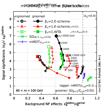
	jet $p_{t}$ cut [GeV]
method	500	1000	1500	2000	2500	3000
mMDT	0.63	0.62	0.62	0.63	0.64	0.65
SoftDrop	0.74	0.74	0.75	0.76	0.77	0.79
Y${}_{\text{m}}$-splitter+trimming	0.49	0.41	0.36	0.33	0.31	0.30
SoftDrop+Y${}_{\text{m}}$-splitter	0.56	0.55	0.55	0.55	0.57	0.58
mMDT + $\tau_{21,\text{groomed}}^{\text{dichroic}}<1$	0.60	0.57	0.58	0.58	0.59	0.61
all other variants	0.4	0.4	0.4	0.4	0.4	0.4

Table 1: Signal efficiencies for the various tools shown in Fig. 13.

Let us start by examining the pure mMDT result: as known already from Dasgupta:2013ihk it provides mild tagging, it has small non-perturbative corrections and only modest dependence on $p_{t}$. SoftDrop ($\beta=2$), when used alone, has slightly lower significance and larger non-perturbative corrections. These two tools have the highest signal efficiencies, of about $63\%$ and $76\%$ respectively at $2\,\text{TeV}$.

Next we examine combinations that involve Y${}_{\text{m}}$-splitter. Recall that this tool undoes the last clustering of a generalised-$k_{t}$($p=\frac{1}{2}$) clustering of the jet constituents, determines $y=\min(p_{t1}^{2},p_{t2}^{2})\Delta R_{12}^{2}/m^{2}$ on the two resulting prongs, and then imposes a cut $y>y_{\text{cut}}$. This cut is similar in its effect to $z_{\text{cut}}$ in mMDT. When used in conjunction with SD (pre-)grooming, the highest-mass emission that passes the SD cut is also the one that is unclustered by Y${}_{\text{m}}$-splitter and so it is required to pass the $y_{\text{cut}}$ condition. As a result, the constraint in the Lund plane turns out, at the leading-log level, to be identical to that obtained with $\tau_{21,\text{groomed}}^{\text{dichroic}}$ and the condition $\tau_{\text{cut}}=1$, with a Sudakov suppression vetoing all emission down to a mass scale $\rho$ in the SD-groomed jet, and a small prefactor $\sim\alpha_{s}\ln(1/y_{\text{cut}})$. This is reflected in Fig. 13, where one sees that the $\tau_{21,\text{groomed}}^{\text{dichroic}}<1$ curve (black open diamonds) is remarkably similar to the SD+Y${}_{\text{m}}$-splitter curve (red open squares). Where the $\tau_{21,\text{groomed}}^{\text{dichroic}}$ variable has an advantage is that one can now further adjust the choice $\tau_{\text{cut}}$, whereas with SD+Y${}_{\text{m}}$-splitter that freedom is not available.

Of the various Y${}_{\text{m}}$ combination considered in Ref. ourYsplitter , the one that gave the best signal-to-background discrimination was Y${}_{\text{m}}$ with trimming, shown as red solid squares in Fig. 13. Overall it performs less well than the mMDT plus $\tau_{21,\text{groomed}}^{\text{dichroic}}$ combination with $\epsilon_{S}$ fixed to $0.4$, even though is has a broadly similar signal efficiency.

Another point to discuss concerns the choice of $\beta_{\tau}$ in the $N$-subjettiness definition, Eq. (2). Many experimental uses of $N$-subjettiness ratios have concentrated on the choice $\beta_{\tau}=1$, while throughout this article we have used $\beta_{\tau}=2$. A discussion of the $\beta_{\tau}=1$ case is given in Appendix A, including comparisons of dichroic and normal variants. Dichroic always perform best also for $\beta_{\tau}=1$, and so in the brief summary that we give here we will only show dichroic results.

An argument often given for the choice of $\beta_{\tau}=1$ is that it is less sensitive to non-perturbative effects. Fig. 13 (right) shows groomed (filled symbols, solid lines) and ungroomed (open symbols, dashed lines) results for $\beta_{\tau}=1$ (squares and triangles) and $\beta_{\tau}=2$ (circles). For the $\beta_{\tau}=1$ case, we have considered either exclusive-$k_{t}$ axes with the standard $E$-scheme four-vector recombination (triangles), or the exclusive-$k_{t}$ axes with the winner-takes-all (WTA) recombination scheme (squares) Bertolini:2013iqa ; Larkoski:2014uqa ; GPSUnpublished . In both the SD-groomed and ungroomed cases, the non-perturbative corrections are somewhat smaller for $\beta_{\tau}=1$ (except in the WTA groomed case). In the ungroomed case, $\beta_{\tau}=1$ also leads to better signal-discrimination. However once SD-grooming is included the signal discrimination is best for the $\beta_{\tau}=2$ case. If one is concerned about the slightly larger non-perturbative effects for the SD-groomed $\beta_{\tau}=2$ case, then one can slightly increase the $\tau_{\text{cut}}$ choice: in Fig. 11(right) where $\tau_{\text{cut}}$ was chosen so as to obtain a higher signal efficiency of $\epsilon_{S}=0.5$ the $\tau_{21,\text{groomed}}^{\text{dichroic}}$($\beta_{\tau}=2$) performance is very similar to the $\tau_{21,\text{groomed}}^{\text{dichroic}}$($\beta_{\tau}=1$,$\epsilon_{S}=0.4$) performance in Fig. 13(right). Therefore, it is the SD-groomed, $\beta_{\tau}=2$, dichroic ratio that appears to give the best overall performance.

There are a number of other variables that one might also consider, notably energy-correlation functions (ECFs) Larkoski:2013eya ; Larkoski:2014gra ; Moult:2016cvt . In particular we expect that dichroic ratios may be of use also for the most recent set of ECFs discussed in Ref. Moult:2016cvt , a number of which are designed to have similarities to $N$-subjettiness. Their study is, however, beyond the scope of this work.

5 Brief analytic calculations

Figure 14: Lund diagrams associated with various analytic calculations. Left: the basic building block $T_{\alpha}$, Eq. (11), used to write all Sudakov exponents. Centre: representation of the full jet Sudakov $R_{\text{full}}(\rho,\tau_{\text{cut}},z)$, Eq. (13a), including secondary emissions. Right: representation of the full jet Sudakov $R_{\text{SD}}(\rho,\tau_{\text{cut}},z)$, Eq. (13c), including secondary emissions. For both the centre and right plots, the dot indicated by $z$ corresponds to the emission dominating the jet mass and we will integrate over allowed values of its momentum fraction $z$.

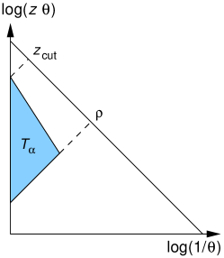
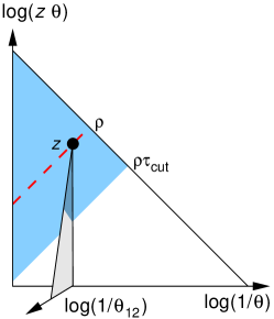
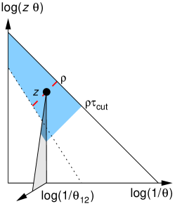
In this Section, we consider brief analytic calculations relating to the observables we have presented so far. Our main goal here is to illustrate that the discussion from Section 3 — where we used Lund diagrams to motivate dichroic subjettiness ratios — does indeed capture the qualitative picture observed in Monte-Carlo simulations. To that aim, it is sufficient to use leading-logarithmic accuracy, where we control double logarithms, i.e. $\alpha_{s}^{n}\ln^{j}\!\rho\ln^{k}\!\rho\ln^{\ell}\!{z_{\text{cut}}}\ln^{m}\!{\zeta_{\text{cut}}}$ with $j+k+\ell+m=2n$, assuming $\rho,\tau_{\text{cut}},z_{\text{cut}},\zeta_{\text{cut}}\ll 1$. Note that, recently, several jet substructure methods have been understood at higher accuracy, see e.g. Frye:2016aiz ; Larkoski:2015kga , and we intend to provide a more precise calculation in future work tau21-calculation .

In practice, we will express everything in terms of the following fundamental block (cf. Fig. 14(left)):

$$T_{\alpha}(\rho,z_{\text{cut}};C_{R})=\int_{0}^{1}\frac{d\theta^{2}}{\theta^{2}}\int_{0}^{1}\frac{dz}{z}\frac{\alpha_{s}(z\theta p_{t}R)C_{R}}{\pi}\Theta(z\theta^{2}>\rho)\Theta(z<z_{\text{cut}}\theta^{\alpha})\Theta(\rho<z_{\text{cut}})\,,$$ (11)

where angles are normalised to the jet radius $R$ and we use the 1-loop running-coupling prescription, $\alpha_{s}(z\theta p_{t}R)=\alpha_{s}/(1+2\alpha_{s}\beta_{0}\log z\theta)$ with $\alpha_{s}\equiv\alpha_{s}(p_{t}R)$ and $\beta_{0}=(11C_{A}-4n_{f}T_{R})/(12\pi)$. Explicit expressions for $T_{\alpha}$ are given in Appendix B and are mostly taken from Ref. Dasgupta:2015lxh . Note that $T_{\alpha}(\rho,z_{\text{cut}};C_{R})=0$ for $z_{\text{cut}}<\rho$.

For the QCD background, we find, for $\tau_{\text{cut}}<1$:

$$\rho_{\text{full}},\>\tau_{21}^{\text{full}}: \!\!\left.\frac{\rho}{\sigma}\frac{d\sigma}{d\rho}\right|_{<\tau_{\text{cut}}}\! \!=\int_{\rho}^{b_{i}}\frac{dz}{z}\frac{\alpha_{s}(\sqrt{z\rho}p_{t}R)C_{R}}{\pi}\exp\big{[}\!-\!R_{\text{full}}(\rho,\tau_{\text{cut}},z)\big{]},$$ (12a)

$$\rho_{\text{mMDT}},\>\tau_{21}^{\text{tagged}}: \!\!\left.\frac{\rho}{\sigma}\frac{d\sigma}{d\rho}\right|_{<\tau_{\text{cut}}}\! \!=\int_{z_{\text{cut}}}^{b_{i}}\frac{dz}{z}\frac{\alpha_{s}(\sqrt{z\rho}p_{t}R)C_{R}}{\pi}\exp\big{[}\!-\!R_{\text{mMDT}}(\rho,\tau_{\text{cut}},z)\big{]},$$ (12b)

$$\rho_{\text{SD}},\>\tau_{21,\text{groomed}}^{\text{full}}: \!\!\left.\frac{\rho}{\sigma}\frac{d\sigma}{d\rho}\right|_{<\tau_{\text{cut}}}\! \!=\int_{z_{\text{SD}}(\rho)}^{b_{i}}\frac{dz}{z}\frac{\alpha_{s}(\sqrt{z\rho}p_{t}R)C_{R}}{\pi}\exp\big{[}\!-\!R_{\text{SD}}(\rho,\tau_{\text{cut}},z)\big{]},$$ (12c)

$$\rho_{\text{mMDT}},\>\tau_{21}^{\text{dichroic}}: \!\!\left.\frac{\rho}{\sigma}\frac{d\sigma}{d\rho}\right|_{<\tau_{\text{cut}}}\! \!=\int_{z_{\text{cut}}}^{b_{i}}\frac{dz}{z}\frac{\alpha_{s}(\sqrt{z\rho}p_{t}R)C_{R}}{\pi}\exp\big{[}\!-\!R_{\text{full}}(\rho,\tau_{\text{cut}},z)\big{]},$$ (12d)

$$\rho_{\text{mMDT}},\>\tau_{21,\text{groomed}}^{\text{dichroic}}: \!\!\left.\frac{\rho}{\sigma}\frac{d\sigma}{d\rho}\right|_{<\tau_{\text{cut}}}\! \!=\int_{z_{\text{cut}}}^{b_{i}}\frac{dz}{z}\frac{\alpha_{s}(\sqrt{z\rho}p_{t}R)C_{R}}{\pi}\exp\big{[}\!-\!R_{\text{SD}}(\rho,\tau_{\text{cut}},z)\big{]},$$ (12e)

where $z_{\text{SD}}(\rho)={\text{max}}\big{(}(\rho^{\beta}\zeta_{\text{cut}}^{2})^{1/(2+\beta)},\rho\big{)}$ and (cf. Fig. 14(middle,right))

$$R_{\text{full}}(\rho,\tau,z) =T_{0}(\tau\rho,b_{i};C_{R})+T_{0}(\sqrt{z\rho}\tau,\sqrt{z\rho}b_{g};C_{A}),$$ (13a)

$$R_{\text{mMDT}}(\rho,\tau,z) =R_{\text{full}}(\rho,\tau,z)-T_{0}(\tau\rho,z_{\text{cut}};C_{R})+T_{0}(\sqrt{z\rho}\tau,z_{\text{cut}}\sqrt{\rho/z};C_{R}),$$ (13b)

$$R_{\text{SD}}(\rho,\tau,z) =R_{\text{full}}(\rho,\tau,z)-T_{\beta}(\tau\rho,\zeta_{\text{cut}};C_{R})+T_{\beta}(\sqrt{z\rho}\tau,\zeta_{\text{cut}}(\rho/z)^{(\beta+1)/2};C_{R}).$$ (13c)

Note that the full and mMDT jet mass Sudakov introduced respectively in Eq. (5) and Eq. (7) (and used below) can be written as

$$R_{\text{full}}(\rho) =R_{\text{full}}(\rho,1,\text{``any }z\text{''})\,,$$ (14a)

$$R_{\text{mMDT}}(\rho) =R_{\text{mMDT}}(\rho,1,\text{``any }z\text{''})\,.$$ (14b)

In the above expressions, $z$ corresponds to the momentum fraction of the emission dominating the jet mass (emission “a” in Figs. 4 and 5). Compared to the simple $R^{\prime}$ factor that we had in Section 2.2, we keep the $z$ integration explicit since the secondary emissions, the $C_{A}$ terms, depend explicitly on $z$. In all cases, the integration over $z$ runs over the region kinematically allowed by the tagger defining the jet mass. The Sudakov exponent in these expressions is then essentially given by the jet on which we compute $\tau_{2}$.

While we only target leading-logarithmic accuracy, our results also include the single-logarithmic contributions coming from hard collinear splittings, which are often phenomenologically important. They appear as the $b_{i}$ factors in Eqs. (12) and (13), where we have introduced $b_{i}=\exp(B_{i})$ with $B_{q}=-3/4$ and $B_{g}=-(11C_{A}-4n_{f}T_{R})/(12C_{A})$. These contributions can effectively be taken into account by limiting all $z$ integrations to $b_{i}$ for primary emissions and $b_{g}$ for secondary emissions.

Finally, as expected, if one takes the limit $\beta\to\infty$ of the SD results, one recovers the full results. Also, the limit $\beta\to 0$ of (12c), reduces to (12b).

So far, we have not yet discussed the case where $\rho$ is computed from the mMDT-tagged jet and $\tau_{21}$ from the full jet. This is more involved due to the two separate kinematic configurations involved (see Fig. 4(b-c)). In the end, we find (assuming $\rho<z_{\text{cut}}$)

$$\rho_{\text{mMDT}},\>\tau_{21}^{\text{full}}:\left.\frac{\rho}{\sigma}\frac{d\sigma}{d\rho}\right|_{<\tau_{\text{cut}}}=\int_{z_{\text{cut}}}^{b_{i}}\frac{dz}{z}\frac{\alpha_{s}(\sqrt{z\rho}p_{t}R)C_{R}}{\pi}\exp\big{[}-R_{\text{full}}(\rho,\tau_{\text{cut}},z)\big{]}\\ +\Theta\left(z_{\text{cut}}>\frac{\rho}{\tau_{\text{cut}}}\right)\int_{z_{\text{cut}}}^{b_{i}}\frac{dz}{z}\frac{\alpha_{s}(\sqrt{z\rho}p_{t}R)C_{R}}{\pi}\exp\big{[}-R_{\text{mMDT}}(\rho)\big{]}\times\\ \times\int_{\rho/\tau_{\text{cut}}}^{z_{\text{cut}}}\frac{d\rho_{c}}{\rho_{c}}\int_{\rho_{c}}^{z_{\text{cut}}}\frac{dz_{c}}{z_{c}}\frac{\alpha_{s}(\sqrt{z_{c}\rho_{c}}p_{t}R)C_{R}}{\pi}\exp\big{[}-R_{\text{out,full}}(\rho_{c},\tau_{\text{cut}},z_{c})\big{]},$$ (15)

and a similar expression with “full” replaced by “SD” for the case where $\tau_{21}$ is calculated on the SD jet. In the above expression, we have used $\rho_{c}=z_{c}\theta_{c}^{2}$ and

$$R_{\text{out,full}}(\rho_{c},\tau,z_{c}) =T_{0}(\rho_{c}\tau,z_{\text{cut}};C_{R})+T_{0}(\sqrt{\rho_{c}z_{c}}\tau,\sqrt{\rho_{c}z_{c}}b_{g};C_{A})\,,$$ (16a)

$$R_{\text{out,SD}}(\rho_{c},\tau,z_{c}) =R_{\text{out,full}}(\rho_{c},\tau,z_{c})$$

$$-T_{\beta}(\rho_{c}\tau,\zeta_{\text{cut}};C_{R})+T_{\beta}(\sqrt{\rho_{c}z_{c}}\tau,\zeta_{\text{cut}}(\rho_{c}/z_{c})^{(\beta+1)/2};C_{R}).$$ (16b)

The configurations contributing to the last two lines of Eq. (15) come from jets with at least one emission in region C (discarded by mMDT) with $\rho_{c}\equiv z_{c}\theta_{c}^{2}>\rho/\tau_{\text{cut}}$. They result in an extra contribution to the mass distribution, which would then be larger than what we obtain with our dichroic combination (Eq. (12d) or, equivalently, the first line of Eq. (15)). When using the dichroic combination, these configurations would all have $\tau_{21}\geq 1$ (up to $\tau_{21}=z_{\text{cut}}/\rho$). In particular, for a cut $\tau_{21}<\tau_{\text{cut}}$ with $\tau_{\text{cut}}>1$, the dichroic combination leads to:

$$\rho_{\text{mMDT}},\>\tau_{21}^{\text{dichroic}}:\left.\frac{\rho}{\sigma}\frac{d\sigma}{d\rho}\right|_{<\tau_{\text{cut}}}\overset{\tau_{\text{cut}}>1}{=}\int_{z_{\text{cut}}}^{b_{i}}\frac{dz}{z}\frac{\alpha_{s}(\sqrt{z\rho}p_{t}R)C_{R}}{\pi}\exp\big{[}-R_{\text{mMDT}}(\rho)\big{]}$$ (17)

$$\bigg{(}\exp\big{[}-R_{\text{out,full}}(\rho\tau_{\text{cut}})\big{]}+\int_{\rho\tau_{\text{cut}}}^{z_{\text{cut}}}\frac{d\rho_{c}}{\rho_{c}}\int_{\rho_{c}}^{z_{\text{cut}}}\frac{dz_{c}}{z_{c}}\frac{\alpha_{s}(\sqrt{z_{c}\rho_{c}}p_{t}R)C_{R}}{\pi}\exp\big{[}-R_{\text{out,full}}(\rho_{c},\rho\tau_{\text{cut}}/\rho_{c},z_{c})\big{]}\bigg{)}$$

with

$$R_{\text{out,full}}(\rho\tau) =T_{0}(\rho\tau,z_{\text{cut}};C_{R})$$ (18a)

$$R_{\text{out,SD}}(\rho\tau) =R_{\text{out,full}}(\rho\tau)-T_{\beta}(\rho\tau,\zeta_{\text{cut}};C_{R}).$$ (18b)

This result splits into 2 contributions corresponding to the two terms in the round bracket on the second line of (17): the first term comes from configurations where there is no emission in region C with $z\theta^{2}>\rho\tau_{\text{cut}}$, and it corresponds to values of $\tau_{21}^{\text{dichroic}}<1$ (this is manifest, because in Eq. (17), given for $\tau_{\text{cut}}>1$, it has no dependence on $\tau_{\text{cut}}$). For the second contribution, the part corresponding to values of $\tau_{21}^{\text{dichroic}}\geq 1$, there is an emission “c” with $z_{c}\theta_{c}^{2}>\rho\tau_{\text{cut}}$. To guarantee $\tau_{21}<\tau_{\text{cut}}$, we then need to veto emissions (both primary and secondary) with $z\theta^{2}>\rho\tau_{\text{cut}}$. Note that this second contribution itself includes two sub-contributions: the case where emission “c” is the only emission in region C with $z\theta^{2}>\rho$, yielding a contribution to the $\tau_{21}$ distribution proportional to $\delta(\tau_{21}-1)$ (recall that $\tau_{2}^{\text{full}}$ is set by the second hardest emission overall, which makes it equal to $\tau_{1}^{\text{tagged}}$); and a second sub-contribution where, in addition to emission “c”, there is at least one additional emission with $\rho\tau_{\text{cut}}>z\theta^{2}>\rho$, yielding a continuum with $\tau_{21}>1$ in the $\tau_{21}$ distribution (see Fig. 7 as well as the right plot of Fig. 15 below). One can calculate the $\delta(\tau_{21}-1)$ contribution to the $\tau_{21}$ distribution by taking the difference between (17) and (12d) for $\tau_{\text{cut}}\to 1$ which gives

$$\int_{z_{\text{cut}}}^{b_{i}}\frac{dz}{z}\frac{\alpha_{s}(\sqrt{z\rho}p_{t}R)C_{R}}{\pi}\int_{\rho}^{z_{\text{cut}}}\frac{d\rho_{c}}{\rho_{c}}\int_{\rho_{c}}^{z_{\text{cut}}}\frac{dz_{c}}{z_{c}}\frac{\alpha_{s}(\sqrt{z_{c}\rho_{c}}p_{t}R)C_{R}}{\pi}e^{-R_{\text{full}}(\rho)-R_{C_{A}}(\rho_{c},z_{c},\rho)},$$ (19)

with $R_{\text{full}}(\rho)$ the full jet mass Sudakov, Eq. (14a), and $R_{C_{A}}(\rho_{c},z_{c},\rho)=T_{0}(\sqrt{z_{c}/\rho_{c}}\rho,\sqrt{\rho_{c}z_{c}}b_{g};C_{A})$. Eq. (19) is equal to the $\tau_{\text{cut}}\to 1$ limit of the second term in round brackets in Eq. (17). In practice the $\delta$-function contribution gets smeared out to values of $\tau_{12}>1$ through the effect of multiple emissions.

Note that it is relatively straightforward to check that the limit $\tau_{\text{cut}}\to 1$ in Eq. (15), or the limit $\tau_{\text{cut}}\to z_{\text{cut}}/\rho$ in Eq. (17) both tend to the mMDT jet mass distribution.

From the equations above, the $\tau_{21}$ distribution, for a given jet mass, can be obtained by taking the derivative with respect to $\tau_{\text{cut}}$ and normalising by the jet mass distribution without any cut on $\tau_{21}$. Background efficiencies can also be obtained straightforwardly by integrating any of the above mass distributions over the allowed mass window.

For signal jets, we assume that if the jet mass is not within some reasonable window around the boson mass, then the jet is discarded. We then find the following signal efficiency

$$\epsilon_{S}=f_{\text{ISR}}\int_{z_{\text{min}}}^{1-z_{\text{min}}}dz\,p_{\text{sig}}(z)\exp\big{[}-R_{\text{sig}}(\rho,\tau_{\text{cut}},z)\big{]},$$ (20)

with $z_{\text{min}}=\rho$, $z_{\text{SD}}(\rho)$ or $z_{\text{cut}}$ depending on whether the mass is computed on the full jet, the SD-groomed jet or the mMDT-tagged jet, respectively. The $\tau_{21}$ distribution for a given jet mass can be obtained by taking the derivative of $\epsilon_{S}$ with respect to $\tau_{\text{cut}}$ (and normalising appropriately).

In Eq. (20) the Sudakov exponent is given by

$$R_{\text{sig}}(\rho,\tau,z) =\Big{[}T_{0}(\sqrt{z(1-z)\rho}\tau;\sqrt{(1-z)\rho/z}b_{i};C_{R})$$

$${\phantom{=}}-T_{0}(\sqrt{z\rho/(1-z)};\sqrt{(1-z)\rho/z}b_{i};C_{R})\Big{]}$$

$$+\Big{[}T_{0}(\sqrt{z(1-z)\rho}\tau;\sqrt{z\rho/(1-z)}b_{i};C_{R})$$

$${\phantom{=}}-T_{0}(\sqrt{(1-z)\rho/z};\sqrt{z\rho/(1-z)}b_{i};C_{R})\Big{]},$$ (21)

valid for small $\tau$. Here we target double-logarithmic accuracy, $\alpha_{s}^{n}\ln^{2n}\tau$, though we also include a set of finite-$z$ and hard-splitting corrections that were found to be numerically important in Ref. Dasgupta:2015lxh (cf. Eq. (A.24)). These represent only a subset of next-to-leading logarithmic terms. Note that for $z\ll 1$ ($1-z\ll 1$) the term on the fourth (second) line is zero because of the last of the $\Theta$-functions in Eq. (11), while the term on the third (first) line corresponds to the leaf in Fig. 3(right). For simplicity, in our numerical results we will use $p_{\text{sig}}(z)=1$ in Eq. (20).

Eq. (20) also includes a factor $f_{\text{ISR}}$ that accounts for the effect of initial-state radiation (ISR). Such effects are present both for signal and background jets and are generically single-logarithmic. As such they are subleading compared to the double-logarithms that we resum.

Nevertheless, if we consider signal jets and examine the limit of large $p_{t}$ with $M$, $\tau_{\text{cut}}$, etc. all fixed, then because of the absence of double logarithms of $\rho$, single-logarithmic ISR effects $(\alpha_{s}\ln\rho)^{n}$ can be numerically dominant Dasgupta:2015yua . Physically, they are associated with the requirement that ISR should not substantially modify the mass of the signal jet. The correction involves $(\alpha_{s}\ln\rho)^{n}$ terms, only when the mass is determined on the full jet and the factor $f_{\text{ISR}}$ then takes the form

$$f_{\text{ISR}} =\exp\Big{[}-\frac{C_{R}}{2\pi\beta_{0}}R^{2}\,\log\frac{1}{1-2\lambda}\Big{]},$$ (22)

$$\lambda =\beta_{0}\alpha_{s}(p_{t})\left[\log\frac{1}{\rho}+{\cal O}\left(\log\frac{M}{\delta M},\log\frac{1}{\tau_{\text{cut}}},\cdots\right)\right],$$ (23)

where a non-global contribution (formally of the same logarithmic order) is ignored for simplicity. In the above formula, $\delta M$ is size of the mass window in which signal jets are accepted, and a full treatment of all single-logarithmic corrections would need to account also for logarithms of $\delta M/M$. A more complete treatment of $f_{\text{ISR}}$ would be relevant for precise phenomenological applications. The finite ${\cal O}\left(\alpha_{s}\right)$ component associated with high-$p_{t}$ emissions could be obtained e.g. using POWHEG powheg , aMC@NLO Alwall:2014hca or at NNLO using MATRIX deFlorian:2016uhr or MCFM mcfm .

Figure 15: Same as figure as 8 and 7 now obtained from our analytic calculation instead of Monte-Carlo simulations. In the right-hand plot, for clarity, the $\delta$-function that appears at $\tau_{21,\text{groomed}}^{\text{dichroic}}=1$ (dijets) has been represented with finite width and scaled down by a factor of $5$.

Figure 16: Same as figure as 9 now obtained from our analytic calculation instead of Monte-Carlo simulations.

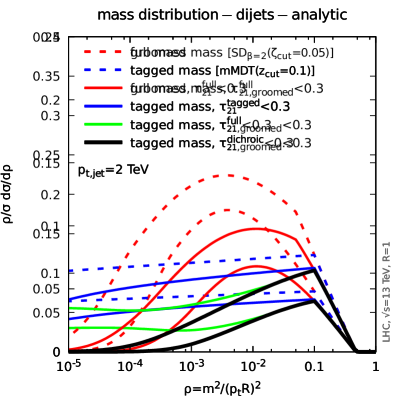
We can now compare our analytic predictions with the Monte-Carlo results from the previous Section. We use $\alpha_{s}(M_{Z})=0.1383$, as in the Pythia 8 simulations presented in the previous Section, and freeze the coupling for scales below $\mu_{\text{fr}}=\tilde{\mu}_{\text{fr}}p_{t}R$, which we set to 1 GeV. We start with the QCD mass distributions, shown on the left plot of Fig. 15, to be compared to the Monte-Carlo results presented in Fig. 8. Globally, we see that our analytic calculation captures correctly the main patterns discussed earlier. We note however that the analytic distributions, especially those involving the full jet mass, are less peaked than the Monte-Carlo ones. This is likely due to subleading logarithmic corrections, like multiple-emission corrections which would effectively increase the Sudakov exponent.

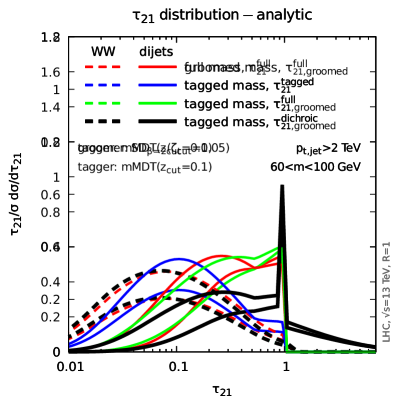
The $\tau_{21}$ distributions for both QCD jets and signal ($W$) jets are shown in the right plot of Fig. 15, to be compared with Fig. 7. The ordering between the different curves is well captured by our analytic expressions. Differences related to the over-simplicity of our leading-logarithmic approximation are larger than what was seen for the mass distribution. First, our analytic calculations are non-zero when $\tau_{21}\to 1$. This region is however not under control within our strongly-ordered approximation. Similarly, the kink observed for $\tau_{21}\sim 0.5$ is not physical. It comes from the onset of the secondary-emission contribution which starts, in our formulas, at $\tau_{21}=b_{g}$. The analytic calculation for our dichroic combination is given by the black curves in the right plot of Fig. 15. The dijet case clearly has a contribution proportional to $\delta(\tau_{21}-1)$ (cf. Eq. (19)) (scaled down by a factor of $5$ for clarity), which is not observed in the Monte-Carlo results. In practice, additional emissions at smaller $z\theta^{2}$ would also contribute to $\tau_{21}$, and they would transform the $\delta(\tau_{21}-1)$ contribution into a Sudakov peak at $\tau_{21}\gtrsim 1$, which is visible on the Monte-Carlo simulations. We are currently working on a better analytic calculation, lifting the assumption that emissions are strongly ordered in $z\theta^{2}$ tau21-calculation .

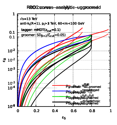
Finally, let us turn to the ROC curves, plotted in Fig. 16. We again see that they reproduce the main qualitative features observed in Section 4. There are however quantitative differences between our analytic results and the Monte-Carlo simulations. For example, our calculation over-estimates the signal efficiencies. A more quantitative description would require a more precise analytic treatment including subleading corrections, beyond the strong-ordering approximation, and fixed-order corrections for signal efficiencies.

6 Conclusion

In this paper we have examined the interplay between boosted-object tagging algorithms, mMDT or SoftDrop, and radiation constraints, notably as imposed through $N$-subjettiness cuts. The analysis points to a new $N$-subjettiness ratio, $\tau_{21}^{\text{dichroic}}=\tau_{2}^{\text{full}}/\tau_{1}^{\text{tagged}}$, where the numerator is evaluated on the full jet, while the denominator is evaluated on the set of constituents left after the tagging stage. The name “dichroic” comes from the fact that the large-angle colour flow, present in backgrounds but not signals, gets directed exclusively to the numerator and not the denominator. It is this feature that leads to an enhanced significance in distinguishing (colour-singlet) signals from (colour-triplet or octet) backgrounds, notably compared to current widely used $N$-subjettiness ratios.

As well as considering signal-significance, it is important to keep non-perturbative effects under control: a method that is overly reliant on non-perturbative physics for its discrimination power is one for which signal-efficiency and background-rejection estimates may be highly model-dependent, and correspondingly uncertain. It is also likely to be subject to large detector effects. We have found that the combination of $\tau_{21}^{\text{dichroic}}$ with a light grooming step based on SoftDrop ($\beta=2$), $\tau_{21,\text{groomed}}^{\text{dichroic}}=\tau_{2}^{\text{SD}}/\tau_{1}^{\text{tagged}}$ is effective in maintaining good signal-to-background significance while substantially limiting non-perturbative effects.

The overall behaviour of our dichroic $\tau_{21}$ variable, with grooming, was illustrated in Fig. 7: the $\tau_{21}$ distribution for signal jets is left largely unmodified by the change to a dichroic variant (black dashed curve versus any of the other dashed curves), whereas the distribution for background jets is shifted to substantially higher values of $\tau_{21}$ (black solid curve versus any of the other solid curves), increasing the ability to distinguish signal and background.

Figures 11 and 13 provide a summary of the signal-significance (vertical axis) and non-perturbative corrections (horizontal axis) for a range of boosted-object identification methods. The points along the lines correspond to different signal-efficiency working points (Fig. 11(left)) or $p_{t}$ cuts (the other plots). One sees that $\tau_{21,\text{groomed}}^{\text{dichroic}}$ with $\beta_{\tau}=2$, in black, provides the best signal significance of any of the methods and that, for a given signal significance, it tends to limit the size of non-perturbative effects relative to other methods.

In addition to the Lund-plane based arguments given in section 3 and the Monte Carlo studies of section 4, we have also outlined the analytic leading-logarithmic structure of different combinations of taggers and $\tau_{21}$ ratios. As well as bringing insight into the behaviour of different taggers, such calculations provide a basis for the future design of “decorrelated” Dolen:2016kst combinations of taggers and dichroic radiation constraints, providing background rejection that is independent of the tagged jet mass and thus straightforward to use in the context of data-driven background estimates.

Appendix A Dichroic subjettiness ratios for $\beta_{\tau}=1$

In Section 3, we have argued in favour of the dichroic subjettiness ratios using $N$-subjettiness with $\beta_{\tau}=2$. In this appendix, we briefly discuss the case $\beta_{\tau}=1$, for which the dichroic variant can also be considered. Note that for $\beta_{\tau}=1$, we have defined the $N$-subjettiness axes through an exclusive-$k_{t}$ declustering. This can be done either using the standard $E$-scheme four-vector recombination or the winner-takes-all (WTA) recombination scheme. For simplicity, we will focus on $E$-scheme results here. A brief comparison between the two axis choices is shown in Fig. 13(right).

Figure 17: ROC curves providing a comparison between different $N$-subjettiness ratios for $\beta_{\tau}=1$ (dashed lines) and $\beta_{\tau}=2$ (solid lines). The same 4 variants as in Figs. 9 and 10 are included. The left (right) column corresponds to full (SD-groomed) jets. The top (bottom) row corresponds to parton-level (hadron-level) events.

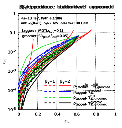
Fig. 17 shows ROC curves similar to those presented in Figs. 9 and 10, this time including results for $\beta_{\tau}=1$ as dashed lines.

We can make several observations based on these plots. First, as for $\beta_{\tau}=2$, we see that the dichroic ratio also outperforms the other combination for $\beta_{\tau}=1$. The performance gain is however smaller, especially with SD grooming.

In terms of the sensitivity to non-perturbative effects, we see that $N$-subjettiness ratios with $\beta_{\tau}=1$ are rather stable even without any SD grooming step. This small sensitivity to non-perturbative effects might have been anticipated since the corresponding $k_{t}$ cut is less affected by soft-and-large-angle emissions than for $\beta_{\tau}=2$. A consequence of this observation is that grooming is less critical when using a cut on $N$-subjettiness ratios with $\beta_{\tau}=1$, and without SD grooming the dichroic combination shows a more sizeable performance gain compared to the other approaches, cf. the bottom-left plot of Fig. 17.

Finally, we can argue that $\beta_{\tau}=2$ gives somewhat better performance than $\beta_{\tau}=1$. To be fair, the comparison should be made between $\tau_{21,\text{groomed}}^{\text{dichroic}}$ for $\beta_{\tau}=2$ (the solid black line on the bottom-right plot of Fig. 17) and $\tau_{21}^{\text{dichroic}}$ for $\beta_{\tau}=1$ (the dashed black line on the bottom-left plot) which both show good signal significance and limited non-perturbative corrections. This comparison shows a somewhat larger background rejection in the $\beta_{\tau}=2$ case for typical signal efficiencies in the $0.2{-}0.6$ range, as also seen in Fig. 13.

Appendix B Explicit expressions for the analytic results

For completeness, we give the result of the building block used for all the analytic calculations in Section 5, see Eq. (11).

We work with a one-loop running coupling (with 5 active flavours), appropriate at our accuracy. We take $\alpha_{s}(M_{Z})=0.1383$ to match with our Pythia simulations and freeze the coupling below a scale $\mu_{\text{fr}}=\tilde{\mu}_{\text{fr}}p_{t}R$ which we set to 1 GeV in practice. We then find

$$T_{\alpha}(\rho,\rho_{0};C_{R}) \overset{L<L_{\text{fr}}}{\makebox[42.67912pt]{$=$}}\frac{C_{R}}{2\pi\alpha_{s}\beta_{0}^{2}}\bigg{[}\frac{W(1-\lambda_{0})}{1+\alpha}+W(1-\lambda)-\frac{2+\alpha}{1+\alpha}W(1-\bar{\lambda})\bigg{]}$$ (24)

$$\overset{\bar{L}<L_{\text{fr}}<L}{\makebox[42.67912pt]{$=$}}\frac{C_{R}}{2\pi\alpha_{s}\beta_{0}^{2}}\bigg{[}\frac{W(1-\lambda_{0})}{1+\alpha}+(1-\lambda)\log(1-\lambda_{\text{fr}})-\frac{2+\alpha}{1+\alpha}W(1-\bar{\lambda})+\lambda_{\text{fr}}-\lambda\bigg{]}$$

$$\makebox[42.67912pt]{ }+\frac{\alpha_{s}(\mu_{\text{fr}})C_{R}}{\pi}(L-L_{\text{fr}})^{2}$$ (25)

$$\overset{L_{0}<L_{\text{fr}}<\bar{L}}{\makebox[42.67912pt]{$=$}}\frac{C_{R}}{2\pi\alpha_{s}\beta_{0}^{2}}\frac{1}{1+\alpha}\bigg{[}W(1-\lambda_{0})-(1-\lambda_{0})\log(1-\lambda_{\text{fr}})+\lambda_{0}-\lambda_{\text{fr}}\bigg{]}$$

$$\makebox[42.67912pt]{ }+\frac{\alpha_{s}(\mu_{\text{fr}})C_{R}}{\pi}\bigg{[}(L-\bar{L})^{2}+\frac{1}{1+\alpha}(\bar{L}-L_{\text{fr}})(\bar{L}+L_{\text{fr}}-2L_{0})\bigg{]}$$ (26)

$$\overset{L_{0}>L_{\text{fr}}}{\makebox[42.67912pt]{$=$}}\frac{\alpha_{s}(\mu_{\text{fr}})C_{R}}{\pi}\frac{1}{2+\alpha}(L-L_{0})^{2},$$ (27)

with $W(x)=x\log(x)$ and

$$L =\log(1/\rho), \lambda =2\alpha_{s}\beta_{0}L,$$ (28)

$$L_{0} =\log(1/\rho_{0}), \lambda_{0} =2\alpha_{s}\beta_{0}L_{0},$$ (29)

$$L_{\text{fr}} =\log(1/\tilde{\mu}_{\text{fr}}), \lambda_{\text{fr}} =2\alpha_{s}\beta_{0}L_{\text{fr}},$$ (30)

$$\bar{L} =\frac{L_{0}+(1+\alpha)L}{2+\alpha}, \bar{\lambda} =2\alpha_{s}\beta_{0}\bar{L}.$$ (31)

Appendix C Example code for dichroic subjettiness ratios

In this last Appendix, we briefly indicate how dichroic subjettiness ratios can be implemented using tools available in FastJet and fjcontrib.

First, besides standard FastJet headers needed for jet clustering, one needs to include the following headers:

⬇

#include <fastjet/contrib/ModifiedMassDropTagger.hh> // mMDT tagger

#include <fastjet/contrib/SoftDrop.hh> // optional SD grooming

#include <fastjet/contrib/Nsubjettiness.hh> // tau1 and tau2

Then, one should declare the basic objects needed for tagging, computing $\tau_{1}$ and $\tau_{2}$, and, optionally, grooming:

⬇

// the tagger [here mMDT with a z cut]

// Note: by default, this automatically reclusters with Cambridge/Aachen

double zcut = 0.1;

fastjet::contrib::ModifiedMassDropTagger mmdt_tagger(zcut);

// (optional) groomer [here SoftDrop]

// Note: by default, this automatically reclusters with Cambridge/Aachen

double beta = 2.0;

double zetacut = 0.05;

fastjet::contrib::SoftDrop sd_pre_groomer(beta, zetacut);

// N-subjettiness with beta_tau=2 and gen-kt axes

double beta_tau = 2.0;

fastjet::contrib::UnnormalizedMeasure measure(beta_tau);

fastjet::contrib::GenKT_Axes axes_gkt(1.0/beta_tau);

fastjet::contrib::Nsubjettiness tau1(1, axes_gkt, measure);

fastjet::contrib::Nsubjettiness tau2(2, axes_gkt, measure);

Note that all parameters here are given as examples and have not been optimised. Also, when used with events contaminated by pileup, a proper pileup mitigation technique should be implemented. This can for example be done by passing a fastjet::Subtractor to the mMDT and SD via the set_subtractor method, and using a GenericSubtractor Soyez:2012hv or a ConstituentSubtractor Berta:2014eza for the $N$-subjettiness variables. Alternatively one can use methods that carry out event-wide pileup-suppression such as PUPPI Bertolini:2014bba or SoftKiller Cacciari:2014gra .

Finally, for a given jet (jet in the example below), one can compute the dichroic subjettiness ratio using

⬇

fastjet::PseudoJet jet; // given jet

fastjet::PseudoJet pre_groomed_jet = sd_pre_groomer(jet); // grooming

fastjet::PseudoJet tagged_jet = mmdt_tagger(pre_groomed_jet); // tagging

double tau1_tagged = tau1(tagged_jet); // $\tau_{1}^{\text{tagged}}$

double tau2_groomed = tau2(pre_groomed_jet); // $\tau_{2}^{\text{groomed}}$

double tagged_mass = tagged_jet.m(); // tagged mass

double tau21_dichroic = tau2_groomed/tau1_tagged; // $\tau_{21,\text{groomed}}^{\text{dichroic}}$

References

- (1) J. M. Butterworth, A. R. Davison, M. Rubin and G. P. Salam, Phys. Rev. Lett. 100 (2008) 242001 [arXiv:0802.2470 [hep-ph]].
- (2) M. Dasgupta, A. Fregoso, S. Marzani and G. P. Salam, JHEP 1309 (2013) 029 [arXiv:1307.0007 [hep-ph]].
- (3) A. J. Larkoski, S. Marzani, G. Soyez and J. Thaler, JHEP 1405 (2014) 146 [arXiv:1402.2657 [hep-ph]].
- (4) J. Thaler and K. Van Tilburg, JHEP 1103 (2011) 015 [arXiv:1011.2268 [hep-ph]].
- (5) J. H. Kim, Phys. Rev. D 83 (2011) 011502 [arXiv:1011.1493 [hep-ph]].
- (6) J. Thaler and K. Van Tilburg, JHEP 1202 (2012) 093 [arXiv:1108.2701 [hep-ph]].
- (7) J. K. Behr, D. Bortoletto, J. A. Frost, N. P. Hartland, C. Issever and J. Rojo, Eur. Phys. J. C 76 (2016) no.7, 386 [arXiv:1512.08928 [hep-ph]].
- (8) G. Aad et al. [ATLAS Collaboration], JHEP 1603 (2016) 127 [arXiv:1512.03704 [hep-ex]].
- (9) V. Khachatryan et al. [CMS Collaboration], Eur. Phys. J. C 76 (2016) no.7, 371 [arXiv:1602.08762 [hep-ex]].
- (10) J. Dolen, P. Harris, S. Marzani, S. Rappoccio and N. Tran, JHEP 1605 (2016) 156 [arXiv:1603.00027 [hep-ph]].
- (11) V. Khachatryan et al. [CMS Collaboration], arXiv:1607.05764 [hep-ex].
- (12) M. Dasgupta, L. Schunk and G. Soyez, JHEP 1604 (2016) 166 [arXiv:1512.00516 [hep-ph]].
- (13) M. Cacciari, G. P. Salam and G. Soyez, JHEP 0804 (2008) 063 [arXiv:0802.1189 [hep-ph]].
- (14) M. Cacciari, G. P. Salam and G. Soyez, Eur. Phys. J. C 72 (2012) 1896 [arXiv:1111.6097 [hep-ph]].
- (15) A. J. Larkoski, D. Neill and J. Thaler, JHEP 1404 (2014) 017 [arXiv:1401.2158 [hep-ph]].
- (16) B. Andersson, G. Gustafson, L. Lonnblad and U. Pettersson, Z. Phys. C 43 (1989) 625.
- (17) C. Frye, A. J. Larkoski, M. D. Schwartz and K. Yan, JHEP 1607 (2016) 064 [arXiv:1603.09338 [hep-ph]].
- (18) A. J. Larkoski, G. P. Salam and J. Thaler, JHEP 1306 (2013) 108 [arXiv:1305.0007 [hep-ph]].
- (19) A. J. Larkoski, I. Moult and D. Neill, JHEP 1412 (2014) 009 [arXiv:1409.6298 [hep-ph]].
- (20) I. Moult, L. Necib and J. Thaler, arXiv:1609.07483 [hep-ph].
- (21) J. Gallicchio and M. D. Schwartz, Phys. Rev. Lett. 107 (2011) 172001 [arXiv:1106.3076 [hep-ph]].
- (22) J. Gallicchio and M. D. Schwartz, JHEP 1304 (2013) 090 [arXiv:1211.7038 [hep-ph]].
- (23) J. R. Andersen et al., arXiv:1605.04692 [hep-ph].
- (24) M. Dasgupta, A. Powling and A. Siodmok, JHEP 1508 (2015) 079 [arXiv:1503.01088 [hep-ph]].
- (25) M. Dasgupta, A. Powling, L. Schunk and G. Soyez, arXiv:1609.07149 [hep-ph].
- (26) A. Altheimer et al., Eur. Phys. J. C 74 (2014) no.3, 2792 [arXiv:1311.2708 [hep-ex]].
- (27) M. Cacciari and G. P. Salam, Phys. Lett. B 659 (2008) 119 [arXiv:0707.1378 [hep-ph]].
- (28) M. Cacciari, G. P. Salam and G. Soyez, JHEP 0804 (2008) 005 [arXiv:0802.1188 [hep-ph]].
- (29) ATLAS Collaboration, “Tagging and suppression of pileup jets,” ATL-PHYS-PUB-2014-001.
- (30) M. Cacciari, G. P. Salam and G. Soyez, Phys. Rev. D 92 (2015) no.1, 014003 [arXiv:1404.7353 [hep-ph]].
- (31) D. Krohn, M. D. Schwartz, M. Low and L. T. Wang, Phys. Rev. D 90 (2014) no.6, 065020 [arXiv:1309.4777 [hep-ph]].
- (32) P. Berta, M. Spousta, D. W. Miller and R. Leitner, JHEP 1406 (2014) 092 [arXiv:1403.3108 [hep-ex]].
- (33) M. Cacciari, G. P. Salam and G. Soyez, Eur. Phys. J. C 75 (2015) no.2, 59 [arXiv:1407.0408 [hep-ph]].
- (34) D. Bertolini, P. Harris, M. Low and N. Tran, JHEP 1410 (2014) 059 [arXiv:1407.6013 [hep-ph]].
- (35) T. Sjostrand, S. Mrenna and P. Z. Skands, Comput. Phys. Commun. 178 (2008) 852 [arXiv:0710.3820 [hep-ph]].
- (36) M. Cacciari and G. P. Salam, Phys. Lett. B 641 (2006) 57 [hep-ph/0512210].
- (37) FastJet Contrib, http://fastjet.hepforge.org/contrib .
- (38) G. P. Salam, L. Schunk and G. Soyez, in preparation.
- (39) J. M. Butterworth, B. E. Cox and J. R. Forshaw, Phys. Rev. D 65 (2002) 096014 [hep-ph/0201098].
- (40) D. Bertolini, T. Chan and J. Thaler, JHEP 1404 (2014) 013 [arXiv:1310.7584 [hep-ph]].
- (41) Gavin P. Salam, unpublished.
- (42) A. J. Larkoski, I. Moult and D. Neill, JHEP 1605 (2016) 117 [arXiv:1507.03018 [hep-ph]].
- (43) J. F. Gunion and Z. Kunszt, Phys. Rev. D 33 (1986) 665.
- (44) P. Nason, JHEP 0411 (2004) 040 [hep-ph/0409146]; S. Frixione, P. Nason and C. Oleari, JHEP 0711 (2007) 070 [arXiv:0709.2092 [hep-ph]]; S. Alioli, P. Nason, C. Oleari and E. Re, JHEP 1006 (2010) 043 [arXiv:1002.2581 [hep-ph]].
- (45) J. Alwall et al., JHEP 1407 (2014) 079 [arXiv:1405.0301 [hep-ph]].
- (46) D. de Florian, M. Grazzini, C. Hanga, S. Kallweit, J. M. Lindert, P. Maierhöfer, J. Mazzitelli and D. Rathlev, JHEP 1609 (2016) 151 [arXiv:1606.09519 [hep-ph]].
- (47) J. M. Campbell and R. K. Ellis, Phys. Rev. D 60 (1999) 113006 [hep-ph/9905386]; J. M. Campbell, R. K. Ellis and C. Williams, JHEP 1107 (2011) 018 [arXiv:1105.0020 [hep-ph]]; R. Boughezal, J. M. Campbell, R. K. Ellis, C. Focke, W. Giele, X. Liu, F. Petriello and C. Williams, arXiv:1605.08011 [hep-ph].
- (48) G. Soyez, G. P. Salam, J. Kim, S. Dutta and M. Cacciari, Phys. Rev. Lett. 110 (2013) no.16, 162001 [arXiv:1211.2811 [hep-ph]].