Enhancing the Physical Layer Security of Non-orthogonal Multiple Access in Large-Scale Networks

Abstract

This paper investigates the physical layer security of non-orthogonal multiple access (NOMA) in large-scale networks with invoking stochastic geometry. Both single-antenna and multiple-antenna aided transmission scenarios are considered, where the base station (BS) communicates with randomly distributed NOMA users. In the single-antenna scenario, we adopt a protected zone around the BS to establish an eavesdropper-exclusion area with the aid of careful channel-ordering of the NOMA users. In the multiple-antenna scenario, artificial noise is generated at the BS for further improving the security of a beamforming-aided system. In order to characterize the secrecy performance, we derive new exact expressions of the security outage probability for both single-antenna and multiple-antenna aided scenarios. To obtain further insights, 1) for the single antenna scenario, we perform secrecy diversity order analysis of the selected user pair. The analytical results derived demonstrate that the secrecy diversity order is determined by the specific user having the worse channel condition among the selected user pair; and 2) for the multiple-antenna scenario, we derive the asymptotic secrecy outage probability, when the number of transmit antennas tends to infinity. Monte Carlo simulations are provided for verifying the analytical results derived and to show that: i) The security performance of the NOMA networks can be improved by invoking the protected zone and by generating artificial noise at the BS; and ii) The asymptotic secrecy outage probability is close to the exact secrecy outage probability.

I Introduction

The unprecedented expansion of new Internet-enabled smart devices, applications and services is expediting the development of the fifth generation (5G) networks, which aim for substantially increasing the throughput of the fourth generation (4G) networks. In addition to the key technologies such as large-scale multiple-input multiple-output (MIMO) solutions, heterogeneous networks and millimeter wave, as well as novel multiple access (MA) techniques should be invoked for improving the spectral efficiency. The existing MA techniques can be primarily classified into two main categories, namely orthogonal multiple access and non-orthogonal multiple access (NOMA), by distinguishing whether a specific resource block can be occupied by more than one user [2]. More specifically, upon investigating the multiplexing gain gleaned from the different domains, the NOMA technique can be further classified as code-domain NOMA and power-domain NOMA [3]. Power-domain NOMA, which has been recently proposed for the 3GPP Long Term Evolution (LTE) initiative [4], is deemed to have a superior spectral efficiency [5, 6]. It has also been pointed out that NOMA has the potential to be integrated with existing MA paradigms, since it exploits the new dimension of the power domain. The key idea of NOMA is to ensure that multiple users can be served within a given resource slot (e.g., time/frequency), by applying successive interference cancellation (SIC). The concept of SIC, which was first proposed by Cover in 1972 [7], constitutes a promising technique, since it imposes lower complexity than the joint decoding approach [8].

Hence NOMA techniques have received remarkable attention both in the world of academia and industry [9, 10, 11, 12, 13]. Ding et al. [9] investigated the performance of the NOMA downlink for randomly roaming users. It was shown that NOMA is indeed capable of achieving a better performance than their traditional orthogonal multiple access (OMA) counter parts. By considering the user fairness of a NOMA system, a user-power allocation optimization problem was addressed by Timotheou and Krikidis [10]. A cooperative simultaneous wireless power transfer (SWIPT) aided NOMA protocol was proposed by Liu et al. [11], where a NOMA user benefitting from good channel conditions acts as an energy harvesting source in order to assist a NOMA user suffering from poor channel conditions. With the goal of maximizing the energy efficiency of transmission in multi-user downlink NOMA scenarios, Zhang et al. [14] proposed an efficient power allocation technique capable of supporting the data rate required by each user. To further improve the performance of NOMA systems, multiple antennas were introduced in [12, 13]. More particularly, the application of multiple-input single-output (MISO) solution to NOMA was investigated by Choi et al. [12], where a two-stage beamforming strategy was proposed. Power optimization was invoked by Sun et al. [13] for maximizing the ergodic capacity of MIMO aided NOMA systems. As a further advance, a massive multiple-input multiple-output (MIMO) aided hybrid heterogenous NOMA framework was proposed for downlink transmission by Liu et al. [15]. The impact of the locations of users and interferers was investigated by using stochastic geometry approaches.

Given the broadcast nature of wireless transmissions, the concept of physical (PHY) layer security (PLS) was proposed by Wyner as early as 1975 from an information-theoretical perspective [16]. This research topic has sparked of wide-spread recent interests. To elaborate, PLS has been considered from a practical perspective in [17, 18, 17, 19, 20, 21]. Specifically, robust beamforming transmission was conceived in conjunction with applying artificial noise (AN) for mitigating the impact of imperfect channel state information (CSI) in MIMO wiretap channels was proposed by Mukherjee and Swindlehurst [17]. Ding et al. [18] invoked relay-aided cooperative diversity for increasing the capacity of the desired link. More particularly, the impact of eavesdroppers on the diversity and multiplexing gains was investigated both in single-antenna and multiple-antenna scenarios. Additionally, the tradeoffs between secure performance and reliability in the presence of eavesdropping attacks was identified by Zou et al. [20]. Furthermore, the physical layer security of D2D communication in large-scale cognitive radio networks was investigated by Liu et al. [21] with invoking a wireless power transfer model, where the positions of the power beacons, the legitimate and the eavesdropping nodes were modeled using stochastic geometry.

Recently, various PHY layer techniques, such as cooperative jamming [22] and AN [23] aided solutions were proposed for improving the PLS, even if the eavesdroppers have better channel conditions than the legitimate receivers. A popular technique is to generate AN at the transmitter for degrading the eavesdroppers’ reception, which was proposed by Goel and Negi in [23]. In contrast to the traditional view, which regards noise and interference as a detrimental effect, generating AN at the transmitter is capable of improving the security, because it degrades the channel conditions of eavesdroppers without affecting those of the legitimate receivers. An AN-based multi-antenna aided secure transmission scheme affected by colluding eavesdroppers was considered by Zhou and McKay [24] for the scenarios associated both with perfect and imperfect CSI at both the transmitter and receiver. As a further development, the secrecy enhancement achieved in wireless Ad Hoc networks was investigated by Zhang et al. [25], with the aid of both beamforming and sectoring techniques. By simultaneously considering matched filter precoding and AN generation techniques, the secure transmission strategies for a multi-user massive MIMO systems was investigated by Wu et al. [26]. Very recently, the PLS of a single-input single-output (SISO) NOMA system was studied by Zhang et al. [27], with the objective of maximizing the secrecy sum rate of multiple users.

I-A Motivation and Contribution

As mentioned above, PLS has been studied in various scenarios, but there is still a paucity of research contributions on investigating the security issues of NOMA, which motivates this contribution. Note that the employment of SIC in NOMA results in a unique interference status at the receivers, which makes the analysis of the PLS of NOMA different from that of OMA. In this paper, we specifically consider the scenario of large-scale networks, where a base station (BS) supports randomly roaming NOMA users. In order to avoid sophisticated high-complexity message detection at the receivers, a user pairing technique is adopted for ensuring that only two users share a specific orthogonal resource slot, which can be readily separated by low-complexity SIC. A random number of eavesdroppers are randomly positioned on an infinite two-dimensional plane according to a homogeneous Poisson point process (PPP). An eavesdropper-exclusion zone is introduced around the BS for improving the secrecy performance of the large-scale networks considered in which no eavesdroppers are allowed to roam. This ‘disc’ was referred to as a protected zone in [28, 29, 25]. Specifically, we consider both a single-antenna scenario and a multiple-antenna scenario at the base station (BS). 1) For the single-antenna scenario, $M$ NOMA users are randomly roaming in an finite disc (user zone) with the quality-order of their channel conditions known at the BS. For example, the $m$-th NOMA user is channel-quality order of $m$. In this case, the $m$-th user is paired with the $n$-th user for transmission within the same resource slot; 2) For the multiple-antenna scenario, we invoke beamforming at the BS for generating AN. In order to reduce the complexity of channel ordering of MISO channels for NOMA, we partitioned the circular cell of Fig. 1 into an internal disc and an external ring. We select one user from the internal disc and another from the external ring to be paired together for transmission within the same resource slot using a NOMA protocol. The primary contributions of this paper are as follows:

• We investigate the secrecy performance of large-scale NOMA networks both for a single-antenna aided and a multiple-antenna assisted scenario at the BS. A protected zone synonymously referred to as the eavesdropper-exclusion area, is invoked in both scenarios for improving the PLS. Additionally, we propose to generate AN at the BS in the multiple-antenna aided scenario for further enhancing the secrecy performance.

• For the single-antenna scenario, we derive the exact analytical expressions of the secrecy outage probability (SOP) of the selected pair of NOMA users, when relying on channel ordering. We then further extend on the secrecy diversity analysis and derive the expressions of asymptotic SOP. The results derived confirm that: 1) for the selected pair, the $m$-th user is capable of attaining a secrecy diversity order of $m$; 2) the secrecy diversity order is determined by the one associated with the worse channel condition between the paired users.

• For the multiple-antenna scenario, we derive the exact analytical expressions of the SOP in conjunction with AN generated at the BS. To gain further insights, we assume having a large antenna array and derive the expressions of SOP, when the number of antennas tends to infinity. The results derived confirm that increasing the number of antennas has no effect on the received signal-to-interference-plus-noise ratio (SINR) at the eavesdroppers, when the BS is equipped with a large antenna array.

• It is shown that: 1) the SOP can be reduced both by extending the protected zone and by generating AN at the BS; 2) the asymptotic SOP results of our large antenna array analysis is capable of closely approximating the exact secrecy outage probability; 3) there is an optimal desired signal-power and AN power sharing ratio, which minimizes the SOP in the multi-antenna scenario.

I-B Organization

The rest of the paper is organized as follows. In Section II, a single-antenna transmission scenario is investigated in random wireless networks, where channel ordering of the NOMA users is relied on. In Section III, a multiple-antenna transmission scenario is investigated, which relies on generating AN at the BS. Our numerical results are presented in Section IV for verifying our analysis, which is followed by our conclusions in Section V.

II Physical Layer Security in Random Wireless Networks with Channel Ordering

As shown in Fig. 1, we focus our attention on a secure downlink communication scenario. In the scenario considered, a BS communicates with $M$ legitimate users (LUs) in the presence of eavesdroppers (Eves). We assume that the $M$ users are divided into $M/2$ orthogonal pairs. Each pair is randomly allocated to a single resource block, such as a time slot or an orthogonal frequency band. For simplicity, we only focus our attention on investigating a typical pair of users in this treatise. Random user-pairing is adopted in this work. For each pair, the NOMA transmission protocol is invoked. It is assumed that BS is located at the center of a disc, denoted by $\mathcal{D}$, which has a coverage radius of ${R_{{D}}}$ (which is defined as the user zone for NOMA [9]). The $M$ randomly roaming LUs are uniformly distributed within the disc. A random number of Eves is distributed across an infinite two-dimensional plane, which are assumed to have powerful detection capabilities and can overhear the messages of all orthogonal RBs, i.e. time slots or frequency slots. The spatial distribution of all Eves is modeled using a homogeneous PPP, which is denoted by ${\Phi_{e}}$ and it is associated with the density ${\lambda_{e}}$. It is assumed that the Eves can be detected, provided that they are close enough to BS. Therefore, an Eve-exclusion area having a radius of $r_{p}$ is introduced. Additionally, all channels are assumed to impose quasi-static Rayleigh fading, where the channel coefficients are constant for each transmission block, but vary independently between different blocks.

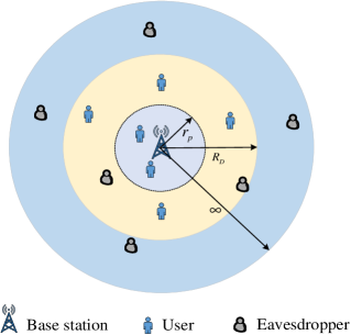
Figure 1: Network model for secure NOMA transmission in single-antenna scenario, where $r_{p}$, $R_{D}$, and $\infty$ is the radius of the Eve-exclusion area, NOMA user zone, and an infinite two dimensional plane for Eves, respectively.

Without loss of generality, it is assumed that all the channels between the BS and LUs obey ${\left|{{h_{1}}}\right|^{2}}\leq\cdot\cdot\cdot{\left|{{h_{m}}}\right|^{2}}\leq\cdot\cdot\cdot{\left|{{h_{n}}}\right|^{2}}\leq\cdot\cdot\cdot{\left|{{h_{M}}}\right|^{2}}$. Both the the small-scale fading and the path loss are incorporated into the ordered channel gain. Again, we assume that the $m$-th user and the $n$-th user ($m<n$) are paired for transmission in the same resource slot. Without loss of generality, we focus our attention on a single selected pair of users in the rest of the paper. In the NOMA transmission protocol, more power should be allocated to the user suffering from worse channel condition [6, 5]. Therefore, the power allocation coefficients satisfy the conditions that ${a_{m}}>{a_{n}}$ and $a_{m}+a_{n}=1$. By stipulating this assumption, SIC can be invoked by the $n$-th user for first detecting the specific user having a higher transmit power (TX-power), who hence has a less interference-infested signal. Accordingly, the $m$-th user’s signal is then remodulated and deducted from the original composite signal. This procedure then directly delivers the decontaminated lower-TX-power signal of the $n$-th user itself. We assume having fixed power allocation sharing between two users, but optimal power sharing strategies are capable of further enhancing the performance of the networks considered, which is beyond the scope of this paper. Based on the aforementioned assumptions, the instantaneous SINR of the $m$-th user and the signal-to-noise ratio (SNR) of the $n$-th user can be written as:

$${\gamma_{{B_{m}}}}=\frac{{{a_{m}}{{\left|{{h_{m}}}\right|}^{2}}}}{{{a_{n}}{{\left|{{h_{m}}}\right|}^{2}}+\frac{1}{\rho_{b}}}},$$ (1)

$${\gamma_{{B_{n}}}}=\rho_{b}{a_{n}}{\left|{{h_{n}}}\right|^{2}},$$ (2)

respectively. We introduce the convenient concept of transmit SNR ${\rho_{b}}=\frac{{{P_{T}}}}{{\sigma_{b}^{2}}}$, where $P_{T}$ is the TX-power of composite signal at the BS and ${\sigma_{b}^{2}}$ is the variance of the additive white Gaussian noise (AWGN) at the LUs, noting that this is not a physically measurable quantity owing to their geographic separation. Perfectly flawless detection is assumed in this treatise, which is realistic at today’s state-of-the-art with the aid of iterative turbo-detection techniques [30, 31]. Additionally, a bounded path loss model is used for guaranteeing that there is a practical path-loss, which is higher than one even for small distances.

We consider the worst-case scenario of large-scale networks, in which the Eves are assumed to have powerful detection capabilities [32, 25]. Specifically, by applying multiuser detection techniques, the multiuser data stream received from BS can be distinguished by the Eves, upon subtracting interference generated by the superposed signals from each other. In fact, this assumption overestimates the Eves’ multi-user decodability. In the scenario considered, all the CSIs of the LUs are assumed to be known at BS. However, the CSIs of Eves are assumed to be unknown at the BS. The most detrimental Eve is not necessarily the nearest one, but the one having the best channel to BS. Non-colluding eavesdroppers are considered in this work. Therefore, the instantaneous SNR of detecting the information of the $m$-th user and the $n$-th user at the most detrimental Eve can be expressed as follows:

$${\gamma_{{E_{\kappa}}}}=\rho_{e}{a_{\kappa}}\mathop{\max}\limits_{e\in{\Phi_{e}},{d_{e}}\geq{r_{p}}}\left\{{{{\left|{{g_{e}}}\right|}^{2}}L\left({{d_{e}}}\right)}\right\}.$$ (3)

It is assumed that $\kappa\in\left\{{m,n}\right\}$, ${\rho_{e}}=\frac{{{P_{T}}}}{{\sigma_{e}^{2}}}$ is the transmit SNR with ${\sigma_{e}^{2}}$ being the variance of the AWGN at Eves. Additionally, ${{{g}_{e}}}$ is defined as the small-scale fading coefficient associated with ${{{{g}_{e}}}}\sim\mathcal{CN}({0,1})$, $L\left({{d_{e}}}\right)=\frac{1}{{d_{e}^{\alpha}}}$ is the path loss, and ${d_{e}}$ is the distance from Eves to BS. Note that due to the existence of the Eve-exclusion area (we assume $r_{p}>1$), it is not required to bound the path loss for Eves since ${d_{e}}$ will always be larger than one.

II-A New Channel Statistics

In this subsection, we derive several new channel statistics for LUs and Eves, which will be used for deriving the secrecy outage probability in the next subsection.

Lemma 1.

Assuming $M$ randomly located NOMA users in the disc of Fig. 1, the cumulative distribution function (CDF) ${F_{{\gamma_{{B_{n}}}}}}$ of the $n$-th LU is given by

$${F_{{\gamma_{{B_{n}}}}}}\left(x\right)\approx{{\varphi_{n}}}\sum\limits_{p=0}^{M-n}{M-n\choose p}\frac{{{{\left({-1}\right)}^{p}}}}{{n+p}}\times$$

$$\sum\limits_{\tilde{S}_{n}^{p}}{{{n+p}\choose{{q_{0}}+\cdots+{q_{K}}}}\left({\prod\limits_{K=0}^{K}{b_{k}^{{q_{k}}}}}\right){e^{-\sum\limits_{k=0}^{K}{{q_{k}}}{c_{k}}\frac{x}{{\rho_{b}{a_{n}}}}}}},$$ (4)

where $K$ is a complexity-vs-accuracy tradeoff parameter, ${b_{k}}=-{\omega_{K}}\sqrt{1-\phi_{k}^{2}}\left({{\phi_{k}}+1}\right)$, ${b_{0}}=-\sum\limits_{k=1}^{K}{{b_{k}}}$, ${c_{k}}=1+{\left[{\frac{{{R_{D}}}}{2}\left({{\phi_{k}}+1}\right)}\right]^{\alpha}}$, ${\omega_{K}}=\frac{\pi}{K}$, ${\phi_{k}}=\cos\left({\frac{{2k-1}}{{2K}}\pi}\right)$, $\tilde{S}_{n}^{p}=\left\{{\left.{\left({{q_{0}},{q_{1}},\cdots,{q_{K}}}\right)}\right|\sum\limits_{i=0}^{K}{{q_{i}}}=n+p}\right\}$, ${n+p\choose{q_{0}}+\cdots+{q_{K}}}=\frac{{\left({n+p}\right)!}}{{{q_{0}}!\cdots{q_{K}}!}}$ and ${\varphi_{n}}=\frac{{M!}}{{\left({M-n}\right)!\left({n-1}\right)!}}$.

Proof.

See Appendix A . ∎

Lemma 2.

Assuming $M$ randomly positioned NOMA users in the disc of Fig. 1, the CDF ${F_{{\gamma_{{B_{m}}}}}}$ of the $m$-th LU is given in (5) at the top of next page,

$${F_{{\gamma_{{B_{m}}}}}}\left(x\right)\approx U\left({x-\frac{{{a_{m}}}}{{{a_{n}}}}}\right)+U\left({\frac{{{a_{m}}}}{{{a_{n}}}}-x}\right){\varphi_{m}}\sum\limits_{p=0}^{M-m}{M-m\choose p}\frac{{{{\left({-1}\right)}^{p}}}}{{m+p}}\sum\limits_{\tilde{S}_{m}^{p}}{{m+p\choose{q_{0}}+\cdots+{q_{K}}}\left({\prod\limits_{k=0}^{K}{b_{k}^{{q_{k}}}}}\right){e^{-\sum\limits_{k=0}^{K}{{q_{k}}{c_{k}}\frac{x}{{\left({{a_{m}}-{a_{n}}x}\right)\rho_{b}}}}}}}.$$ (5)

where $U\left(x\right)=\left\{\begin{array}[]{l}1,x>0\\ 0,x\leq 0\\ \end{array}\right.$ is the unit step function , and $\tilde{S}_{m}^{p}=\left\{{\left.{\left({{q_{0}},{q_{1}},\cdots,{q_{K}}}\right)}\right|\sum\limits_{i=0}^{K}{{q_{i}}}=m+p}\right\}$.

Proof.

Based on (1), the CDF of ${F_{{\gamma_{{B_{m}}}}}}\left(x\right)$ can be expressed as

$${F_{{\gamma_{{B_{m}}}}}}\left(x\right)=\left\{\begin{array}[]{l}\underbrace{\Pr\left\{{{{\left|{{h_{m}}}\right|}^{2}}<\frac{x}{{\left({{a_{m}}-{a_{n}}x}\right)\rho_{b}}}}\right\}}_{{\Phi_{m}}},x<\frac{{{a_{m}}}}{{{a_{n}}}}\\ 1,x\geq\frac{{{a_{m}}}}{{{a_{n}}}}\\ \end{array}\right..$$ (8)

To derive the CDF of ${F_{{\gamma_{{B_{m}}}}}}\left(x\right)$, ${\Phi_{m}}$ can be expressed as ${\Phi_{m}}={F_{{{\left|{{h_{m}}}\right|}^{2}}}}\left({\frac{x}{{\left({{a_{m}}-{a_{n}}x}\right)\rho_{b}}}}\right)$. Based on (Appendix A: Proof of Lemma 1), interchanging the parameters $m\to n$ and applying $y=\frac{x}{{\left({{a_{m}}-{a_{n}}x}\right)\rho_{b}}}$, we obtain

$${\Phi_{m}}={\varphi_{m}}\sum\limits_{p=0}^{M-m}{M-m\choose p}\frac{{{{\left({-1}\right)}^{p}}}}{{m+p}}\times$$

$$\sum\limits_{\tilde{S}_{m}^{p}}{{m+p\choose{q_{0}}+\cdots+{q_{K}}}\left({\prod\limits_{k=0}^{K}{b_{k}^{{q_{k}}}}}\right){e^{-\sum\limits_{k=0}^{K}{{q_{k}}{c_{k}}\frac{x}{{\left({{a_{m}}-{a_{n}}x}\right)\rho_{b}}}}}}}.$$ (9)

By substituting (2) into (8), with the aid of the unit step function, the CDF of ${F_{{\gamma_{{B_{m}}}}}}\left(x\right)$ can be obtained. The proof is completed. ∎

Lemma 3.

Assuming that the eavesdroppers obey the PPP distribution and the Eve-exclusion zone has a radius of $r_{p}$, the probability density function (PDF) ${f_{{\gamma_{{E_{\kappa}}}}}}$ of the most detrimental Eve (where $\kappa\in\left\{{m,n}\right\}$ ) is given by

$${f_{{\gamma_{{E_{\kappa}}}}}}\left(x\right)={\mu_{\kappa 1}}{e^{-\frac{{{\mu_{\kappa 1}}\Gamma\left({\delta,{\mu_{\kappa 2}}x}\right)}}{{{x^{\delta}}}}}}\left({\frac{{\mu_{\kappa 2}^{\delta}{e^{-{\mu_{\kappa 2}}x}}}}{x}+\frac{{\delta\Gamma\left({\delta,{\mu_{\kappa 2}}x}\right)}}{{{x^{\delta+1}}}}}\right),$$ (10)

where ${\mu_{\kappa 1}}=\delta\pi{\lambda_{e}}{\left({{\rho_{e}}{a_{\kappa}}}\right)^{\delta}},{\mu_{\kappa 2}}=\frac{{r_{p}^{\alpha}}}{{{\rho_{e}}{a_{\kappa}}}}$, $\delta=\frac{2}{\alpha}$ and $\Gamma(\cdot,\cdot)$ is the upper incomplete Gamma function.

Proof.

To derive the PDF of ${f_{{\gamma_{{E_{\kappa}}}}}}\left(x\right)$, we have to compute the CDF of ${F_{{\gamma_{{E_{\kappa}}}}}}$ firstly as

$${F_{{\gamma_{{E_{\kappa}}}}}}\left(x\right)= {\mathbb{E}_{{\Phi_{e}}}}\left\{{\prod\limits_{e\in{\Phi_{e}},{d_{e}}\geq{r_{p}}}{{F_{{{\left|{{g_{e}}}\right|}^{2}}}}\left({\frac{{xd_{e}^{\alpha}}}{{\rho_{e}{a_{\kappa}}}}}\right)}}\right\}.$$ (11)

Following the similar approach as [33], by applying the generating function [34], (11) can be rewritten as

$${F_{{\gamma_{{E_{\kappa}}}}}}\left(x\right)= \exp\left[{-{\lambda_{e}}{\int_{{R^{2}}}}\left({1-{F_{{{\left|{{g_{e}}}\right|}^{2}}}}\left({\frac{{xd_{e}^{\alpha}}}{{\rho_{e}{a_{\kappa}}}}}\right)}\right)rdr}\right]$$

$$= \exp\left[{-2\pi{\lambda_{e}}\int_{{r_{p}}}^{\infty}{r{e^{-\frac{x}{{\rho_{e}{a_{\kappa}}}}{r^{\alpha}}}}dr}}\right].$$ (12)

By applying [35, Eq. (3.381.9)], we arrive at:

$${F_{{\gamma_{{E_{\kappa}}}}}}\left(x\right)={e^{-\frac{{\delta\pi{\lambda_{e}}{{\left({\rho_{e}{a_{\kappa}}}\right)}^{\delta}}\Gamma\left({\delta,\frac{{xr_{p}^{\alpha}}}{{\rho_{e}{a_{\kappa}}}}}\right)}}{{{x^{\delta}}}}}}.$$ (13)

By taking the derivative of the CDF ${F_{{\gamma_{{E_{\kappa}}}}}}\left(x\right)$ in (13), we obtain the PDF ${\gamma_{{E_{\kappa}}}}$ in (10). The proof is completed. ∎

II-B Secrecy Outage Probability

In the networks considered, the capacity of the LU’s channel for the $\kappa$-h user ($\kappa\in\left\{{m,n}\right\}$ ) is given by ${C_{{B_{\kappa}}}}={\log_{2}}(1+{\gamma_{{B_{\kappa}}}})$, while the capacity of the Eve’s channel for the $\kappa$-th user is quantified by ${C_{{E_{\kappa}}}}={\log_{2}}(1+{\gamma_{{E_{\kappa}}}})$. It is assumed that the length of the block is sufficiently high for facilitating the employment of capacity-achieving codes within each block. Additionally, the fading block length of the main channel and of the eavesdropper’s channel are assumed to be the same. As such, according to [36], the secrecy rate of the $n$-th and of the $m$-th user can be expressed as

$${C_{n}}={\left[{{C_{{B_{n}}}}-{C_{{E_{n}}}}}\right]^{+}},$$ (14)

$${C_{m}}={\left[{{C_{{B_{m}}}}-{C_{{E_{m}}}}}\right]^{+}},$$ (15)

where we have $[x]^{+}=\mathrm{max}\{x,0\}$. Here, the secrecy rates of LUs are strictly positive [37]. Recall that the Eves’ CSIs are unknown at the BS, hence the BS can only send information to the LUs at a constant rate, but perfect secrecy is not always guaranteed [38]. Considering the $\kappa$-th user as an example, if ${R_{\kappa}}<{C_{\kappa}}$, the information with a rate of $R_{\kappa}$ ($\kappa\in\left\{{m,n}\right\}$ is conveyed in perfect secrecy. By contrast, for the case of ${R_{\kappa}}>{C_{\kappa}}$ the information-theoretic security is compromised. Motivated by this, secrecy outage probability is used as our secrecy performance metric in this paper. Given the expected secrecy rate ${R}_{{\kappa}}$ of the $\kappa$-th user, a secrecy outage event is declared, when the secrecy rate ${C}_{{\kappa}}$ drops below ${R}_{{\kappa}}$, which is defined as the SOP for the $\kappa$-th user. Recall that we have allocated $M$ users to $M/2$ orthogonal RBs, each pair of users are independent from all other pairs of users. We focus our attention on the SOP of a typical pair of users. We then derive the SOP of the $\kappa$-th user in the following two Theorems. We consider the SOP under the condition that the connection between BS and LUs can be established.

Theorem 1.

Assuming that the LUs position obeys the PPP for the ordered channels of the LUs, the SOP of the $n$-th user is given by (1) at the top of this page.

$$P_{n}\left({{R_{n}}}\right)= {\varphi_{n}}\sum\limits_{p=0}^{M-n}{M-n\choose p}\frac{{{{\left({-1}\right)}^{p}}}}{{n+p}}{\sum_{\tilde{S}_{n}^{p}}}{n+p\choose{q_{0}}+\cdots+{q_{K}}}\left({\prod\limits_{K=0}^{K}{b_{k}^{{q_{k}}}}}\right)$$

$$\times\int_{0}^{\infty}{{\mu_{n1}}\left({\frac{{\mu_{n2}^{\delta}{e^{-{\mu_{n2}}x}}}}{x}+\frac{{\delta\Gamma\left({\delta,{\mu_{n2}}x}\right)}}{{{x^{\delta+1}}}}}\right){e^{-\frac{{{\mu_{n1}}\Gamma\left({\delta,{\mu_{n2}}x}\right)}}{{{x^{\delta}}}}-\sum\limits_{k=0}^{K}{{q_{k}}}{c_{k}}\frac{{{2^{{R_{n}}}}\left({1+x}\right)-1}}{{\rho_{b}{a_{n}}}}}}dx}.$$ (16)

Proof.

In this treatise, we consider the SOP under the condition that the connection between the BS and LUs can be established. As such, the SIC has been assumed to be successfully performed at the $n$-th user. Based on (14), the SOP is given by

$$P_{n}\left({{R_{n}}}\right)= \int_{0}^{\infty}{{f_{{\gamma_{{E_{n}}}}}}\left(x\right){F_{{\gamma_{{B_{n}}}}}}\left({{2^{{R_{n}}}}\left({1+x}\right)-1}\right)dx}.$$ (17)

Upon using the results of Lemma 1 and Lemma 3, substituting (1) and (10) into (17), after some further mathematical manipulations, we can express the SOP of the $n$-th user. The proof is completed. ∎

Theorem 2.

Assuming that the LUs position obeys the PPP for the ordered channels of the LUs, the SOP of the $m$-th user is given by (2) at the top of next page,

$$P_{m}\left({{R_{m}}}\right)= 1-{e^{-\frac{{{\mu_{m1}}\Gamma\left({\delta,{\tau_{m}}{\mu_{m2}}}\right)}}{{{\tau_{m}}^{\delta}}}}}+{\varphi_{m}}\sum\limits_{p=0}^{M-m}{M-m\choose p}\frac{{{{\left({-1}\right)}^{p}}}}{{m+p}}{\sum_{\tilde{S}_{m}^{p}}}{m+p\choose{q_{0}}+\cdots+{q_{K}}}\left({\prod\limits_{k=0}^{K}{b_{k}^{{q_{k}}}}}\right)$$

$$\times\int_{0}^{{\tau_{m}}}{{\mu_{m1}}\left({\frac{{\mu_{m2}^{\delta}{e^{-{\mu_{m2}}x}}}}{x}+\frac{{\delta\Gamma\left({\delta,{\mu_{m2}}x}\right)}}{{{x^{\delta+1}}}}}\right){e^{-\frac{{{\mu_{m1}}\Gamma\left({\delta,{\mu_{m2}}x}\right)}}{{{x^{\delta}}}}-\sum\limits_{k=0}^{K}{{q_{k}}{c_{k}}\frac{{{2^{{R_{m}}}}\left({1+x}\right)-1}}{{\left({{a_{m}}-{a_{n}}\left({{2^{{R_{m}}}}\left({1+x}\right)-1}\right)}\right){\rho_{b}}}}}}}dx}.$$ (18)

where we have ${\tau_{m}}=\frac{1}{{{2^{{R_{m}}}}\left({1-{a_{m}}}\right)}}-1$.

Proof.

Based on (15) and according to [37], the SOP for the $m$-th user is given by

$$P_{m}\left({{R_{m}}}\right)= \int_{0}^{\infty}{{f_{{\gamma_{{E_{m}}}}}}\left(x\right){F_{{\gamma_{{B_{m}}}}}}\left({{2^{{R_{m}}}}\left({1+x}\right)-1}\right)dx}.$$ (19)

Upon using the results of Lemma 2 and Lemma 3, as well as substituting (5) and (10) into (19), after some further mathematical manipulations, we can express the SOP of the $m$-th user. The proof is completed. ∎

In this paper, based on the assumptions of perfect SIC of LUs and strong detection capabilities of Eves aforementioned, the secrecy outage occurs in the $m$-th user and the $n$-th user are independent. Note that relaxing these two assumptions requires to consider dependence between two users by discussing more sophisticated connect/secrecy outage events, which should be included in our future work with the aid of the results derived in this paper. In other words, the SOP of the $m$-th user has no effect on the SOP of the $n$-th user and vice versa. As a consequence, we define the SOP for the selected user pair as that of either the $m$-th user or the $n$-th user outage.

Proposition 1.

The SOP of the selected user pair is given by

$$P_{mn}=1-\left({1-P_{m}}\right)\left({1-P_{n}}\right),$$ (20)

where $P_{n}$ and $P_{m}$ are given by (1) and (2), respectively.

II-C Secrecy Diversity Order Analysis

In order to derive the secrecy diversity order to gain further insights into the system’s operation in the high-SNR regime, the following new analytical framework is introduced. Again, as the worst-case scenario, we assume that Eves have a powerful detection capability. The asymptotic behavior is analyzed, usually when the SNR of the channels between the BS and LUs is sufficiently high, i.e., when the BS’s transmit SNR obeys ${\rho_{b}}\to\infty$, while and the SNR of the channels between BS and Eves is set to arbitrary values. It is noted that for the Eve’s transmit SNR of ${\rho_{e}}\to\infty$, the probability of successful eavesdropping will tend to unity. The secrecy diversity order can be defined as follows:

$${d_{s}}=-\mathop{\lim}\limits_{{\rho_{b}}\to\infty}\frac{{\log P^{\infty}}}{{\log{\rho_{b}}}},$$ (21)

where $P^{\infty}$ is the asymptotic SOP.

Corollary 1.

Assuming that the LUs position obeys the PPP for the ordered channels of the LUs, the asymptotic SOP of the $n$-th user is given by

$$P_{n}^{\infty}\left({{R_{n}}}\right) ={G_{n}}{\left({{\rho_{b}}}\right)^{-{D_{n}}}}+o\left({\rho_{b}^{-{D_{n}}}}\right),$$ (22)

where we have ${Q_{1}}=\int_{0}^{\infty}{\mu_{n1}}{e^{-\frac{{{\mu_{n1}}\Gamma\left({\delta,{\mu_{n2}}x}\right)}}{{{x^{\delta}}}}}}\times\\ \left({\frac{{\mu_{n2}^{\delta}{e^{-{\mu_{n2}}x}}}}{x}+\frac{{\delta\Gamma\left({\delta,{\mu_{n2}}x}\right)}}{{{x^{\delta+1}}}}}\right){\left({\frac{{\left({{2^{{R_{n}}}}\left({1+x}\right)-1}\right)\ell}}{{{a_{n}}}}}\right)^{n}}dx$, ${G_{n}}=\frac{{{\varphi_{n}}{Q_{1}}}}{n}$, and ${D_{n}}=n$.

Proof.

We commence our diversity order analysis by characterizing the CDF of the LUs $F_{{\gamma_{{B_{m}}}}}^{\infty}$ and $F_{{\gamma_{{B_{n}}}}}^{\infty}$ in the high-SNR regime. When $y\to 0$, based on (A.3) and the approximation of $1-{e^{-y}}\approx y$, we obtain the asymptotic unordered CDF of ${{{\left|{{{\tilde{h}}_{n}}}\right|}^{2}}}$ as follows:

$$F_{{{\left|{{{\tilde{h}}_{n}}}\right|}^{2}}}^{\infty}\left(y\right) \approx\frac{{2y}}{{R_{D}^{2}}}\int_{0}^{{R_{D}}}{\left({1+{r^{\alpha}}}\right)rdr}=y\ell,$$ (23)

where $\ell=1+\frac{{2R_{D}^{\alpha}}}{{\alpha+2}}$. Substituting (23) into (A.2), the asymptotic unordered CDF of ${{{\left|{{{\tilde{h}}_{n}}}\right|}^{2}}}$ is given by

$$F_{{{\left|{{h_{n}}}\right|}^{2}}}^{\infty}\left(y\right) ={\varphi_{n}}\sum\limits_{p=0}^{M-n}{{M-n}\choose p}\frac{{{{\left({-1}\right)}^{p}}}}{{n+p}}{\left({y\ell}\right)^{n+p}}\approx\frac{{{\varphi_{n}}}}{n}{\left({y\ell}\right)^{n}}.$$ (24)

Then based on (A.1), we can obtain $F_{{\gamma_{B_{n}}}}^{\infty}\left(x\right)\approx\frac{{{\varphi_{n}}}}{n}{\left({\frac{{x\ell}}{{{\rho_{b}}{a_{n}}}}}\right)^{n}}$. Based on (17), we can replace the CDF of ${F_{{\gamma_{{B_{n}}}}}}$ by the asymptotic $F_{{\gamma_{{B_{n}}}}}^{\infty}$. After some manipulations, we arrive at the asymptotic SOP of the $n$-th user. The proof is completed. ∎

Remark 1.

Upon substituting (22) into (21), we obtain the secrecy diversity order of the $n$-th user is $n$.

Corollary 2.

Assuming that the LUs position obeys the PPP for the ordered channels of the LUs, the asymptotic SOP for the $m$-th user is given by

$$P_{m}^{\infty}\left({{R_{n}}}\right) ={G_{m}}{\left({{\rho_{b}}}\right)^{-{D_{m}}}}+o\left({\rho_{b}^{-{D_{m}}}}\right),$$ (25)

where we have ${Q_{2}}=\int_{0}^{{\tau_{m}}}{{\mu_{m1}}{e^{-\frac{{{\mu_{m1}}\Gamma\left({\delta,{\mu_{m2}}x}\right)}}{{{x^{\delta}}}}}}}\times\\ \left({\frac{{\mu_{m2}^{\delta}{e^{-{\mu_{m2}}x}}}}{x}+\frac{{\delta\Gamma\left({\delta,{\mu_{m2}}x}\right)}}{{{x^{\delta+1}}}}}\right){\left({\frac{{\left({{2^{{R_{m}}}}\left({1+x}\right)-1}\right)\ell}}{{\left({{a_{m}}-{a_{n}}\left({{2^{{R_{m}}}}\left({1+x}\right)-1}\right)}\right)}}}\right)^{m}}dx$, ${G_{m}}=\frac{{{\varphi_{m}}{Q_{2}}}}{m}$ and ${D_{m}}=m$.

Proof.

Based on ${\Phi_{m}}$ and (24), we can arrive at:

$$\Phi_{m}^{\infty}\approx \frac{{{\varphi_{m}}}}{m}{\left({\frac{{x\ell}}{{\left({{a_{m}}-{a_{n}}x}\right){\rho_{b}}}}}\right)^{m}}.$$ (26)

Substituting (26) into (8), the asymptotic CDF of ${{\gamma_{{B_{m}}}}}$ can be expressed as

$$F_{{\gamma_{{B_{m}}}}}^{\infty}\left(x\right)=U\left({x-\frac{{{a_{m}}}}{{{a_{n}}}}}\right)+U\left({\frac{{{a_{m}}}}{{{a_{n}}}}-x}\right)\Phi_{m}^{\infty},$$ (27)

where $\Phi_{m}^{\infty}$ is given in (26). Then, based on (19), we can replace the CDF of ${F_{{\gamma_{{B_{m}}}}}}$ by the asymptotic $F_{{\gamma_{{B_{m}}}}}^{\infty}$ of (27). Additionally, we can formulate the asymptotic SOP of the $m$-th user. The proof is completed. ∎

Remark 2.

Upon substituting (25) into (21), we obtain the secrecy diversity order of the $m$-th user is $m$.

Proposition 2.

For $m<n$, the secrecy diversity order can be expressed as

$${d_{s}}=-\mathop{\lim}\limits_{{\rho_{b}}\to\infty}\frac{{\log\left({P_{m}^{\infty}+P_{n}^{\infty}-P_{m}^{\infty}P_{n}^{\infty}}\right)}}{{\log{\rho_{b}}}}=m.$$ (28)

Proof.

Based on Corollary 2 and Corollary 1, and upon substituting (22) and (25) into (20), the asymptotic SOP for the user pair can be expressed as

$$P_{mn}^{\infty}= P_{m}^{\infty}+P_{n}^{\infty}-P_{m}^{\infty}P_{n}^{\infty}\approx P_{m}^{\infty}{G_{m}}{\left({{\rho_{b}}}\right)^{-{D_{m}}}}.$$ (29)

Upon substituting (29) into (21), we arrive at (28). The proof is completed. ∎

Remark 3.

The results of (28) indicate that the secrecy diversity order and the asymptotic SOP for the user pair considered are determined by the $m$-th user.

Remark 3 provides insightful guidelines for improving the SOP of the networks considered by invoking user pairing among of the $M$ users. Since the SOP of a user pair is determined by that of the one having a poor channel, it is efficient to pair the user having the best channel and the second best channel for the sake of achieving an increased secrecy diversity order.

III Enhancing Security with the aid of Artificial Noise

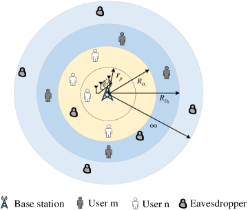
Figure 2: Network model for secure NOMA transmission using AN in multiple-antenna scenario, where $r_{p}$, $R_{D_{1}}$, $R_{D_{2}}$, and $\infty$ is the radius of the Eve-exclusion zone, NOMA user zone for user $n$, NOMA user zone for user $m$, and an infinite two dimensional plane for eavesdroppers, respectively.

In addition to single antenna scenario [1], for further improving the secrecy performance, let us now consider the employment of multiple antennas at BS for generating AN in order to degrade the Eves’ SNR. More particularly, the BS is equipped with $N_{A}$ antennas, while all LUs and Eves are equipped with a single antenna each. Here, ${N_{A}}>2$ is assumed for ensuring the existence of a null-space for two NOMA users. We mask the superposed information of NOMA by superimposing AN on Eves with the aid of the BS. It is assumed that the perfect CSI of LUs are known at BS. Since the AN is in the null space of the intended LU’s channel, it will not impose any effects on LUs. However, it can significantly degrade the channel and hence the capacity of Eves. More precisely, the key idea of using AN as proposed in [39] can be described as follows: an orthogonal basis of $C^{N_{A}}$ is generated at BS for user $\kappa$, (where ${\kappa\in\left\{{m,n}\right\}}$) as a $\left({{N_{A}}\times{N_{A}}}\right)$–element precoding matrix ${{\bf{U}}_{\kappa}}=\left[{{{\bf{u}}_{\kappa}},{{\bf{V}}_{\kappa}}}\right]$, where we have ${{\bf{u}}_{\kappa}}={\raise 3.01385pt\hbox{${\bf{h}_{\kappa}^{\dagger}}$}\!\mathord{\left/{\vphantom{{\bf{h_{\kappa}}^{\dagger}}{\left\|{{\bf{h}_{\kappa}}}\right\|}}}\right.\kern-1.2pt}\!\lower 3.01385pt\hbox{${\left\|{{\bf{h_{\kappa}}}}\right\|}$}}$ , and ${{\bf{V}}_{\kappa}}$ is of size $N_{A}\times\left({N_{A}-1}\right)$. Here, ${\bf{h}_{\kappa}}$ is denoted as the intended channel between the BS and user $\kappa$. It is noted that each column of ${{\bf{V}}_{\kappa}}$ is orthogonal to ${{\bf{u}}_{\kappa}}$. Beamforming is applied at the BS for generating AN. As such, the transmitted superposed information, which is masked by AN at the BS is given by

$$\sum\limits_{\kappa\in\left\{{m,n}\right\}}{\sqrt{{a_{\kappa}}}{{\bf{x}}_{\kappa}}}=\sum\limits_{\kappa\in\left\{{m,n}\right\}}\sqrt{{a_{\kappa}}}\left({{s_{\kappa}}{{\bf{u}}_{\kappa}}+{{\bf{t}}_{\kappa}}{{\bf{V}}_{\kappa}}}\right),$$ (30)

where $s_{\kappa}$ is the information-bearing signal with a variance of $\sigma_{s}^{2}$, and ${{\bf{t}}_{\kappa}}$ is the AN. Here the (${{N_{A}}-1}$) elements of ${{\bf{t}}_{\kappa}}$ are independent identically distributed (i.i.d.) complex Gaussian random variables with a variance of $\sigma_{a}^{2}$. As such, the overall power per transmission is ${P_{T}}={P_{S}}+{P_{A}}$, where ${P_{S}}=\theta{P_{T}}=\sigma_{s}^{2}$ is the transmission power of the desired information-bearing signal, while ${P_{A}}=\left({1-\theta}\right){P_{T}}=\left({{N_{A}}-1}\right)\sigma_{a}^{2}$ is the transmission power of the AN. Here $\theta$ represents the power sharing coefficients between the information-bearing signal and AN.

As shown in Fig. 2, we divide the disc $D$ into two regions, namely, $D_{1}$ and $D_{2}$, respectively. The motivation of using this topology hinges on two aspects. The first one is to create more distinct channel quality differences between the paired users, since existing NOMA studies have demonstrated that it is beneficial to pair two users having rather different channel conditions [5, 40, 11]. The second one is that of reducing the complexity of channel ordering in this MISO NOMA system, which provides a compelling flexibility. By doing so, the path loss is the dominant channel impairment in this scenario, because compared to the instantaneous small-scale fading effects, the path loss is more stable and more dominant. A quantitative example of comparing the small-scale fading and path loss was provided in Chapter 2 of [41]. Note that the proposed design cannot guarantee the optimal ordering for MISO NOMA channels. More sophisticated precoding/detection design strategies (e.g., cluster based design, signal alignment and etc.) can be developed for further enhancing the attainable performance of the networks considered [42, 43], but this is beyond the scope of this treatise. Here, $D_{1}$ is an internal disc with radius $R_{D_{1}}$, and the group of user $n$ is located in this region. $D_{2}$ is an external ring spanning the radius distance from $R_{D_{1}}$ to $R_{D_{2}}$, and the group of user $m$ is located in this region. For simplicity, we assume that user $n$ and user $m$ are the selected user from each group in the rest of this paper. The cell-center user $n$ is assumed to be capable of cancelling the interference of the cell-edge user $m$ using SIC techniques. User $n$ and user $m$ are randomly selected in each region for pairing them for NOMA. The combined signal at user $m$ is given by

$${{\bf{y}}_{m}}=\underbrace{\frac{{{{\bf{h}}_{m}}{{\bf{u}}_{m}}\sqrt{{a_{m}}}{s_{m}}}}{{\sqrt{1+d_{m}^{\alpha}}}}}_{{\bf{Signal}}\;{\bf{part}}}+\underbrace{\frac{{{{\bf{h}}_{m}}{{\bf{u}}_{n}}\sqrt{{a_{n}}}{s_{n}}}}{{\sqrt{1+d_{m}^{\alpha}}}}+\frac{{{{\bf{h}}_{m}}{{\bf{V}}_{n}}\sqrt{{a_{n}}}{{\bf{t}}_{n}}}}{{\sqrt{1+d_{m}^{\alpha}}}}+{{\bf{n}}_{m}}}_{{\bf{Interference}}\;{\bf{and}}\;{\bf{noise}}\;{\bf{part}}},$$ (31)

where ${{\bf{n}}_{m}}$ is a Gaussian noise vector at user $m$, while $d_{m}$ is the distance between the BS and user $m$. Substituting (30) into (31), the received SINR at user $m$ is given by

$$\gamma_{{B_{m}}}^{AN}=\frac{{{a_{m}}\sigma_{s}^{2}{{\left\|{{{\bf{h}}_{m}}}\right\|}^{2}}}}{{{a_{n}}\sigma_{s}^{2}{{\left|{{{\bf{h}}_{m}}\frac{{{\bf{h}}_{n}^{\dagger}}}{{\left\|{{{\bf{h}}_{n}}}\right\|}}}\right|}^{2}}+{a_{n}}\sigma_{a}^{2}{{\left\|{{{\bf{h}}_{m}}{{\bf{V}}_{n}}}\right\|}^{2}}+1+d_{m}^{\alpha}}},$$ (32)

where the variance of ${{\bf{n}}_{m}}$ is normalized to unity. As such, we can express the transmit SNR at BS as $\rho_{t}=P_{T}$.

Since SIC is applied at user $n$, the interference arriving from user $m$ can be detected and subtracted firstly. The aggregate signal at user $n$ is given by

$${{\bf{y}}_{n}}=\underbrace{\frac{{{{\bf{h}}_{n}}{{\bf{u}}_{n}}\sqrt{{a_{n}}}{s_{n}}}}{{\sqrt{1+d_{n}^{\alpha}}}}}_{{\bf{Signal}}\;{\bf{part}}}+\underbrace{\frac{{{{\bf{h}}_{n}}{{\bf{V}}_{m}}\sqrt{{a_{m}}}{{\bf{t}}_{m}}}}{{\sqrt{1+d_{n}^{\alpha}}}}+{{\bf{n}}_{n}}}_{{\bf{Interference}}\;{\bf{and}}\;{\bf{noise}}\;{\bf{part}}},$$ (33)

where ${{\bf{n}}_{n}}$ is the Gaussian noise at user $n$, while $d_{n}$ is the distance between the BS and user $n$. The received SINR at user $n$ is given by

$$\gamma_{{B_{n}}}^{AN}=\frac{{{a_{n}}\sigma_{s}^{2}{{\left\|{{{\bf{h}}_{n}}}\right\|}^{2}}}}{{{a_{m}}\sigma_{a}^{2}{{\left\|{{{\bf{h}}_{n}}{{\bf{V}}_{m}}}\right\|}^{2}}+1+d_{n}^{\alpha}}},$$ (34)

where the variance of ${{\bf{n}}_{n}}$ is normalized to unity. The signal observed by Eves is given by

$${{\bf{y}}_{e}}=\sum\limits_{\kappa\in\left\{{m,n}\right\}}{\frac{{{{\bf{h}}_{e}}\sqrt{{a_{\kappa}}}{{\bf{x}}_{\kappa}}}}{{\sqrt{d_{e}^{\alpha}}}}}+{{\bf{n}}_{e}},$$ (35)

where ${{\bf{n}}_{e}}$ is the Gaussian noises at Eves, while ${{\bf{h}}_{e}}\in{{\mathop{\rm C}\nolimits}^{1\times{N_{A}}}}$ is the channel vector between the BS and Eves. Similar to the single-antenna scenario, again, we assume that the Eves have a strong detection capability and hence they unambiguously distinguish the messages of user $m$ and user $n$. The received SINR of the most detrimental Eve associated with detecting user $\kappa$ is given by

$$\gamma_{{E_{\kappa}}}^{AN}={a_{\kappa}}\sigma_{s}^{2}\mathop{\max}\limits_{e\in{\Phi_{e}},{d_{e}}\geq{r_{p}}}\left\{{\frac{{{{X_{e,\kappa}}}}}{I_{e}^{AN}+d_{e}^{\alpha}}}\right\},$$ (36)

where the variance of ${{\bf{n}}_{e}}$ is normalized to unity, and we have ${X_{e,\kappa}}={\left|{{{\bf{h}}_{e}}\frac{{{\bf{h}}_{\kappa}^{\dagger}}}{{\left\|{{{\bf{h}}_{\kappa}}}\right\|}}}\right|^{2}}$ as well as $I_{e}^{AN}={a_{m}}\sigma_{a}^{2}{\left\|{{{\bf{h}}_{e}}{{\bf{V}}_{m}}}\right\|^{2}}+{a_{n}}\sigma_{a}^{2}{\left\|{{{\bf{h}}_{e}}{{\bf{V}}_{n}}}\right\|^{2}}$.

III-A New Channel Statistics

In this subsection, we derive several new channel statistics for LUs and Eves in the presence of AN, which will be used for deriving the SOP in the next subsection.

Lemma 4.

Assuming that user $n$ is randomly positioned in the disc $D_{1}$ of Fig. 2, the CDF of $F_{{B_{n}}}^{AN}$ is given by

$$F_{{B_{n}}}^{AN}\left(x\right)=1-{b_{2}}{e^{-\frac{{\vartheta x}}{{{a_{m}}}}}}\sum\limits_{p=0}^{{N_{A}}-1}{\frac{{{\vartheta^{p}}{x^{p}}}}{{p!}}}\sum\limits_{q=0}^{p}{p\choose q}\times$$

$$\frac{{\Gamma\left({{N_{A}}-1+q}\right)a_{m}^{q-p}}}{{{{\left({\vartheta x+\frac{{{N_{A}}-1}}{{{P_{A}}}}}\right)}^{{N_{A}}-1+q}}}}\sum\limits_{u=0}^{p-q}{p-q\choose u}\frac{{a_{m}^{u+\delta}\gamma\left({u+\delta,\frac{{\vartheta x}}{{{a_{m}}}}R_{{D_{1}}}^{\alpha}}\right)}}{{{{\left({\vartheta x}\right)}^{u+\delta}}}},$$ (37)

where we have ${b_{2}}=\frac{\delta}{{R_{{D_{1}}}^{2}\Gamma\left({{N_{A}}-1}\right){{\left({\frac{{{P_{A}}}}{{{N_{A}}-1}}}\right)}^{{N_{A}}-1}}}}$ and $\vartheta=\frac{{{a_{m}}}}{{{a_{n}}{P_{S}}}}$.

Proof.

See Appendix B. ∎

Lemma 5.

Assuming that user $m$ is randomly positioned in the ring $D_{2}$ of Fig. 2, for the case of ${\theta\neq\frac{1}{{{N_{A}}}}}$, the CDF of $F_{{B_{m}}}^{AN}$ is given by

$$F_{{B_{m}}}^{AN}\left(x\right)=1-{e^{-\frac{{\nu x}}{{{a_{n}}}}}}\sum\limits_{p=0}^{{N_{A}}-1}{\frac{{{{\left({\nu x}\right)}^{p}}}}{{p!}}}\sum\limits_{q=0}^{p}{p\choose q}a_{n}^{q-p}\times$$

$$\underbrace{{a_{1}}\left({\frac{{\Gamma\left({q+1}\right)}}{{{{\left({\nu x+\frac{1}{{{P_{S}}}}}\right)}^{q+1}}}}-\sum\limits_{l=0}^{{N_{A}}-2}{\frac{{{{\left({\frac{{{N_{A}}-1}}{{{P_{A}}}}-\frac{1}{{{P_{S}}}}}\right)}^{l}}}}{{\frac{{l!{{\left({\nu x+\frac{{{N_{A}}-1}}{{{P_{A}}}}}\right)}^{q+l+1}}}}{{\Gamma\left({q+l+1}\right)}}}}}}\right)}_{{\rm I}\left(\theta\right)}\times$$

$$\sum\limits_{u=0}^{p-q}{p-q\choose u}\frac{{\gamma\left({u+\delta,\frac{{\nu x}}{{{a_{n}}}}R_{{D_{2}}}^{\alpha}}\right)-\gamma\left({u+\delta,\frac{{\nu x}}{{{a_{n}}}}R_{{D_{1}}}^{\alpha}}\right)}}{{{{\left({\frac{{\nu x}}{{{a_{n}}}}}\right)}^{u+\delta}}}},$$ (38)

where $\gamma\left({\cdot,\cdot}\right)$ is the lower incomplete Gamma function, $\Gamma\left({\cdot}\right)$ is the Gamma function, ${a_{1}}=\delta{\left({1-\frac{{{P_{A}}}}{{\left({{N_{A}}-1}\right){P_{S}}}}}\right)^{1-{N_{A}}}}/\left({\left({R_{{D_{2}}}^{2}-R_{{D_{1}}}^{2}}\right){P_{S}}}\right)$, and $\nu=\frac{{{a_{n}}}}{{{a_{m}}{P_{S}}}}$.

For the case of ${\theta=\frac{1}{{{N_{A}}}}}$, the CDF of $F_{{B_{m}}}^{AN}$ is given by (5) upon substituting ${{\rm I}\left(\theta\right)}$ by ${{\rm I}^{*}}\left(\theta\right)$, where we have ${{\rm I}^{*}}\left(\theta\right)=\frac{{{a_{2}}\Gamma\left({q+{N_{A}}}\right)}}{{{{\left({\nu x+\frac{1}{{{P_{S}}}}}\right)}^{q+{N_{A}}}}}}\sum\limits_{u=0}^{p-q}{p-q\choose u}$ and ${a_{2}}=\frac{\delta}{{\left({R_{{D_{2}}}^{2}-R_{{D_{1}}}^{2}}\right){P_{S}}^{{N_{A}}}\left({{N_{A}}-1}\right)!}}$.

Proof.

See Appendix C. ∎

Lemma 6.

Assuming that the distribution of Eves obeys a PPP and that the Eve-exclusion zone has a radius of $r_{p}$, the PDF of ${f_{\gamma_{{E_{\kappa}}}^{AN}}}$ (where ${\kappa\in\left\{{m,n}\right\}}$) is given by

$${f_{\gamma_{{E_{\kappa}}}^{AN}}}\left(x\right)=-{e^{{\Theta_{\kappa}}{\Psi_{\kappa 1}}}}\times$$

$$\left({\frac{{{{\left({\mu_{\kappa 2}^{AN}}\right)}^{\delta}}{e^{-x\mu_{\kappa 2}^{AN}}}}}{x}{\Psi_{\kappa 1}}+\frac{{\delta{\Theta_{\kappa}}{\Psi_{\kappa 1}}}}{x}+{\Theta_{\kappa}}{\Psi_{\kappa 2}}}\right),$$ (39)

where ${\Theta_{\kappa}}=\frac{{\Gamma\left({\delta,x\mu_{\kappa 2}^{AN}}\right)}}{{{x^{\delta}}}}$, $\Gamma\left({\cdot,\cdot}\right)$ is the upper incomplete Gamma function, ${\Psi_{\kappa 1}}=\Omega\frac{1}{{{{\left({\frac{x}{{{a_{\kappa}}{P_{S}}}}+{\tau_{i}}}\right)}^{j}}}},{\Psi_{\kappa 2}}=\Omega\frac{1}{{{{\left({\frac{x}{{{a_{\kappa}}{P_{S}}}}+{\tau_{i}}}\right)}^{j}}}}\left({\frac{j}{{\left({\frac{x}{{{a_{\kappa}}{P_{S}}}}+{\tau_{i}}}\right)}}\frac{1}{{{a_{\kappa}}{P_{S}}}}}\right)$, $\Omega={\left({-1}\right)^{{N_{A}}}}\mu_{\kappa 1}^{AN}\times\\ \prod\limits_{i=1}^{2}{\tau_{i}^{{N_{A}}-1}}\sum\limits_{i=1}^{2}{\sum\limits_{j=1}^{{N_{A}}-1}{{a_{{N_{A}}-j,{N_{A}}-1}}{{\left({2{\tau_{i}}-L}\right)}^{j-\left({2{N_{A}}-2}\right)}}}}$ , $L={\tau_{1}}+{\tau_{2}},{\tau_{1}}=\frac{{{N_{A}}-1}}{{{a_{m}}{P_{A}}}},{\tau_{2}}=\frac{{{N_{A}}-1}}{{{a_{n}}{P_{A}}}}$, ${a_{{N_{A}}-j,{N_{A}}-1}}={2{N_{A}}-j-3\choose{N_{A}}-j-1}$, $\mu_{\kappa 1}^{AN}=\pi{\lambda_{e}}\delta{\left({{a_{\kappa}}{P_{S}}}\right)^{\delta}}$, and $\mu_{\kappa 2}^{AN}=\frac{{r_{p}^{\alpha}}}{{{a_{\kappa}}{P_{S}}}}$.

Proof.

See Appendix D. ∎

III-B Secrecy Outage Probability

In this subsection, we investigate the SOP of a multiple-antenna aided scenario relying on AN.

Theorem 3.

Assuming that the LUs and Eves distribution obey PPPs and that AN is generated at the BS, the SOP of user $n$ is given by (3) at the top of next page,

$$P_{n}^{AN}\left({{R_{n}}}\right) =\int_{0}^{\infty}{-{e^{{\Theta_{n}}{\Psi_{n1}}}}\left({\frac{{{{\left({\mu_{n2}^{AN}}\right)}^{\delta}}{e^{-x\mu_{n2}^{AN}}}}}{x}{\Psi_{n1}}+\frac{{\delta{\Theta_{n}}{\Psi_{n1}}}}{x}+{\Theta_{n}}{\Psi_{n2}}}\right)}$$

$$\times\left({1-{b_{2}}{e^{-{\iota_{n}}}}\sum\limits_{p=0}^{{N_{A}}-1}{\frac{{{\iota_{n*}}}}{{p!}}}\sum\limits_{q=0}^{p}{p\choose q}\frac{{\Gamma\left({{N_{A}}-1+q}\right)a_{m}^{q}}}{{{{\left({{a_{m}}{\iota_{n*}}+\frac{{{N_{A}}-1}}{{{P_{A}}}}}\right)}^{{N_{A}}-1+q}}}}\sum\limits_{u=0}^{p-q}{p-q\choose u}\frac{{\gamma\left({u+\delta,{\iota_{n*}}R_{{D_{1}}}^{\alpha}}\right)}}{{\iota_{n*}^{u+\delta}}}}\right)dx,$$ (40)

where ${\iota_{n*}}=\frac{{\vartheta\left({{2^{{R_{n}}}}\left({1+x}\right)-1}\right)}}{{{a_{m}}}}$.

Proof.

Using the results of Lemma 4 and Lemma 6, upon substituting (4) and (6) into (17), we can obtain the SOP of user $n$. The proof is completed. ∎

Theorem 4.

Assuming that the LUs and Eves distribution obey PPPs and that AN is generated at the BS, for the case $\theta\neq\frac{1}{{{N_{A}}}}$, the SOP of user $m$ is given by (4) at the top of next page,

$$P_{m}^{AN}\left({{R_{m}}}\right) =\int_{0}^{\infty}{-{e^{{\Theta_{m}}{\Psi_{m1}}}}\left({\frac{{{{\left({\mu_{m2}^{AN}}\right)}^{\delta}}{e^{-x\mu_{m2}^{AN}}}}}{x}{\Psi_{m1}}+\frac{{\delta{\Theta_{m}}{\Psi_{m1}}}}{x}+{\Theta_{m}}{\Psi_{m2}}}\right)}$$

$$\times\underbrace{\left({1-a_{1}^{*}\sum\limits_{p=0}^{{N_{A}}-1}{\frac{{\iota_{m}^{p}}}{{p!}}}\sum\limits_{q=0}^{p}{p\choose q}a_{n}^{q}\left({\frac{{\Gamma\left({q+1}\right)}}{{{{\left({{a_{n}}{\iota_{m*}}+\frac{1}{{{P_{S}}}}}\right)}^{q+1}}}}-\sum\limits_{l=0}^{{N_{A}}-2}{\frac{{\frac{1}{{l!}}{{\left({\frac{{{N_{A}}-1}}{{{P_{A}}}}-\frac{1}{{{P_{S}}}}}\right)}^{l}}\Gamma\left({q+l+1}\right)}}{{{{\left({{a_{n}}{\iota_{m*}}+\frac{{{N_{A}}-1}}{{{P_{A}}}}}\right)}^{q+l+1}}}}}}\right){\rm T}_{1}^{*}}\right)}_{{\rm K}\left(\theta\right)}dx,$$ (41)

where we have $a_{1}^{*}=\frac{{\delta{e^{-{\iota_{m*}}}}{{\left({1-\frac{{{P_{A}}}}{{\left({{N_{A}}-1}\right){P_{S}}}}}\right)}^{1-{N_{A}}}}}}{{\left({R_{{D_{2}}}^{2}-R_{{D_{1}}}^{2}}\right){P_{S}}}}$, ${\rm T}_{1}^{*}=\sum\limits_{u=0}^{p-q}{p-q\choose u}\frac{{\gamma\left({u+\delta,{\iota_{m*}}R_{{D_{2}}}^{\alpha}}\right)-\gamma\left({u+\delta,{\iota_{m*}}R_{{D_{1}}}^{\alpha}}\right)}}{{\iota_{m*}^{u+\delta}}}$, and ${\iota_{m*}}=\frac{{\nu\left({{2^{{R_{m}}}}\left({1+x}\right)-1}\right)}}{{{a_{n}}}}$.

For the case of ${\theta=\frac{1}{{{N_{A}}}}}$, the SOP for user $m$ is given by (4) upon substituting ${{\rm K}\left(\theta\right)}$ with ${{\rm K}^{*}}\left(\theta\right)$, where ${{\rm K}^{*}}\left(\theta\right)=1-a_{2}^{*}\sum\limits_{p=0}^{{N_{A}}-1}{\frac{{\iota_{m*}^{p}}}{{p!}}}\sum\limits_{q=0}^{p}{p\choose q}\frac{{\Gamma\left({q+{N_{A}}}\right)a_{n}^{q}}}{{{{\left({{a_{n}}{\iota_{m*}}+\frac{1}{{{P_{S}}}}}\right)}^{q+{N_{A}}}}}}\sum\limits_{u=0}^{p-q}{p-q\choose u}{\rm T}_{1}^{*}$, and $a_{2}^{*}=\frac{{\delta{e^{-{\iota_{m*}}}}}}{{\left({R_{{D_{2}}}^{2}-R_{{D_{1}}}^{2}}\right){P_{S}}^{{N_{A}}}\left({{N_{A}}-1}\right)!}}$.

Proof.

Using the results of Lemma 5 and Lemma 6, upon substituting (5) and (6) into (19), we obtain the SOP of user $m$. The proof is completed. ∎

Proposition 3.

The SOP of multiple-antenna aided scenario relaying on AN for the selected user pair can be expressed as

$$P^{AN}_{mn}=1-\left({1-P^{AN}_{m}}\right)\left({1-P^{AN}_{n}}\right).$$ (42)

where $P_{n}$ and $P_{m}$ are given by (3) and (4), respectively.

III-C Large Antenna Array Analysis

In this subsection, we investigate the system’s asymptotic behavior when the BS is equipped with large antenna arrays. Large antenna arrays using narrow beamforming are potentially capable of distinguishing multiple users in the angular domain [44, 45]. Nonetheless, the users covered by the same narrow beam in dense deployments still remain non-orthogonal [46]. It is noted that for the exact SOP derived in (4) and (3), as $N_{A}$ increases, the number of summations in the equations will increase exponentially, which imposes an excessive complexity. Motivated by this, we seek good approximations for the SOP associated with a large $N_{A}$. With the aid of the theorem of large values, we have the following approximations [24]. $\mathop{\lim}\limits_{{N_{A}}\to\infty}{\left\|{{{\bf{h}}_{n}}}\right\|^{2}}\to{N_{A}}$, $\mathop{\lim}\limits_{{N_{A}}\to\infty}{\left\|{{{\bf{h}}_{m}}}\right\|^{2}}\to{N_{A}}$, $\mathop{\lim}\limits_{{N_{A}}\to\infty}{\left\|{{{\bf{h}}_{n}}{{\bf{V}}_{m}}}\right\|^{2}}\to{N_{A}}-1$, and $\mathop{\lim}\limits_{{N_{A}}\to\infty}{\left\|{{{\bf{h}}_{m}}{{\bf{V}}_{n}}}\right\|^{2}}\to{N_{A}}-1$. We first derive the asymptotic CDF of user $n$ for ${N_{A}}\to\infty$.

Lemma 7.

Assuming that user $n$ is randomly located in the disc $D_{1}$ of Fig. 2 and ${N_{A}}\to\infty$, the CDF of $F_{{B_{n}},\infty}^{AN}$ is given by

$$F_{{B_{n}},\infty}^{AN}\left(x\right)=\left\{\begin{array}[]{l}0,x<{\zeta_{n}}\\ 1-\frac{{{{\left({\frac{{{a_{n}}{P_{S}}{N_{A}}}}{x}-{a_{m}}{P_{A}}-1}\right)}^{\delta}}}}{{R_{{D_{1}}}^{2}}},{\zeta_{n}}\leq x\leq{\xi_{n}}\\ 1,x\geq{\xi_{n}}\\ \end{array}\right.,$$ (46)

where we have ${\zeta_{n}}=\frac{{{a_{n}}{P_{S}}{N_{A}}}}{{R_{{D_{1}}}^{\alpha}+{a_{m}}{P_{A}}+1}}$ and ${\xi_{n}}=\frac{{{a_{n}}{P_{S}}{N_{A}}}}{{{a_{m}}{P_{A}}+1}}$.

Proof.

Based on (34), we can express the asymptotic CDF of $F_{{B_{n}},\infty}^{AN}$ as $F_{{B_{n}},\infty}^{AN}\left(x\right)=\Pr\left\{{\frac{{{a_{n}}{P_{S}}{N_{A}}}}{{{a_{m}}{P_{A}}+1+d_{n}^{\alpha}}}\leq x}\right\}$. After some further mathematical manipulations, we can obtain the CDF of $F_{{B_{n}},\infty}^{AN}$ for large antenna arrays. The proof is completed. ∎

We then derive the asymptotic CDF of user $m$ for ${N_{A}}\to\infty$.

Lemma 8.

Assuming that user $m$ is randomly located in the ring $D_{2}$ of Fig. 2 and ${N_{A}}\to\infty$, the CDF of $F_{{B_{m}},\infty}^{AN}$ is given by

$$F_{{B_{m}},\infty}^{AN}\left(x\right)=\left\{\begin{array}[]{l}1,x\geq{\zeta_{m1}}\\ \frac{{R_{{D_{2}}}^{2}-t_{m}^{2}+{b_{1}}{e^{-\frac{{{a_{m}}{P_{S}}{N_{A}}}}{{x{a_{n}}{P_{S}}}}}}}}{{R_{{D_{2}}}^{2}-R_{{D_{1}}}^{2}}}\\ \times\int_{{R_{{D_{1}}}}}^{{t_{m}}}r{e^{\frac{{{r^{\alpha}}}}{{{a_{n}}{P_{S}}}}}}dr,{\zeta_{m2}}<x\leq{\zeta_{m1}}\\ \frac{{{b_{1}}{e^{-\frac{{{a_{m}}{P_{S}}{N_{A}}}}{{x{a_{n}}{P_{S}}}}}}}}{{R_{{D_{2}}}^{2}-R_{{D_{1}}}^{2}}}\int_{{R_{{D_{1}}}}}^{{R_{{D_{2}}}}}r{e^{\frac{{{r^{\alpha}}}}{{{a_{n}}{P_{S}}}}}}dr,x<{\zeta_{m2}}\\ \end{array}\right.,$$ (51)

where we have $b_{1}=2{e^{\frac{{{a_{n}}{P_{A}}+1}}{{{a_{n}}{P_{S}}}}}}$, ${t_{m}}=\sqrt[\alpha]{{\frac{{{a_{m}}{P_{S}}{N_{A}}}}{x}-{a_{n}}{P_{A}}-1}}$, ${\zeta_{m1}}=\frac{{{a_{m}}{P_{S}}{N_{A}}}}{{R_{{D_{1}}}^{\alpha}+{a_{n}}{P_{A}}+1}},{\zeta_{m2}}=\frac{{{a_{m}}{P_{S}}{N_{A}}}}{{R_{{D_{2}}}^{\alpha}+{a_{n}}{P_{A}}+1}}$, and ${\xi_{m}}=\frac{{{a_{m}}{P_{S}}{N_{A}}}}{{{a_{n}}{P_{A}}+1}}.$

Proof.

Similarly, based on (32),the CDF of the asymptotic $F_{{B_{m}},\infty}^{AN}$ is given by

$$F_{{B_{m}},\infty}^{AN}\left(x\right)=\Pr\left\{{\frac{{{a_{m}}{P_{S}}{N_{A}}}}{{{a_{n}}{P_{S}}{{\left|{{{\bf{h}}_{m}}\frac{{{\bf{h}}_{n}^{\dagger}}}{{\left\|{{{\bf{h}}_{n}}}\right\|}}}\right|}^{2}}+{a_{n}}{P_{A}}+1+d_{m}^{\alpha}}}\leq x}\right\}.$$ (52)

After some further mathematical manipulations, we obtain the CDF of $F_{{B_{m}},\infty}^{AN}$ for large antenna arrays. The proof is completed. ∎

Let us now turn our attention to the derivation of the Eves’ PDF in a large-scale antenna scenario.

Lemma 9.

Assuming that the Eves distribution obeys a PPP and that AN is generated at the BS, the Eve-exclusion zone has a radius of $r_{p}$, and ${N_{A}}\to\infty$, the PDF of ${f_{\gamma_{{E_{\kappa}},\infty}^{AN}}}$ (where ${\kappa\in\left\{{m,n}\right\}}$) is given by

$${f_{\gamma_{{E_{\kappa}},\infty}^{AN}}}\left(x\right)={e^{-\frac{{\mu_{\kappa 1}^{AN}\Gamma\left({\delta,\mu_{\kappa 2}^{AN}x}\right){e^{-\frac{{{P_{A}}x}}{{{a_{\kappa}}{P_{S}}}}}}}}{{{x^{\delta}}}}-\frac{{{P_{A}}x}}{{{a_{\kappa}}{P_{S}}}}}}\mu_{\kappa 1}^{AN}{x^{-\delta}}$$

$$\times\left({{{\left({\mu_{\kappa 2}^{AN}}\right)}^{\delta}}{x^{\delta-1}}{e^{-\mu_{\kappa 2}^{AN}x}}+\Gamma\left({\delta,\mu_{\kappa 2}^{AN}x}\right)\left({\frac{{{P_{A}}}}{{{a_{\kappa}}{P_{S}}}}+\frac{\delta}{x}}\right)}\right).$$ (53)

Proof.

Using the theorem of large values, we have $\mathop{\lim}\limits_{{N_{A}}\to\infty}I_{e,\infty}^{AN}={a_{m}}\sigma_{a}^{2}{\left\|{{{\bf{h}}_{e}}{{\bf{V}}_{m}}}\right\|^{2}}+{a_{n}}\sigma_{a}^{2}{\left\|{{{\bf{h}}_{e}}{{\bf{V}}_{n}}}\right\|^{2}}\to{P_{A}}$. The asymptotic CDF of ${F_{\gamma_{{E_{\kappa}},\infty}^{AN}}}$ associated with ${N_{A}}\to\infty$ is given by

$${F_{\gamma_{{E_{\kappa}},\infty}^{AN}}}\left(x\right)=\Pr\left\{{\mathop{\max}\limits_{e\in{\Phi_{e}},{d_{e}}\geq{r_{p}}}\left\{{\frac{{{a_{\kappa}}{P_{S}}{X_{e,\kappa}}}}{{I_{e,\infty}^{AN}+d_{e}^{\alpha}}}}\right\}\leq x}\right\}$$

$$={E_{{\Phi_{e}}}}\left\{{\prod\limits_{e\in{\Phi_{e}},{d_{e}}\geq{r_{p}}}{{F_{{X_{e,\kappa}}}}\left({\frac{{\left({{P_{A}}+d_{e}^{\alpha}}\right)x}}{{{a_{\kappa}}{P_{S}}}}}\right)}}\right\}.$$ (54)

Following the procedure used for deriving (3), we apply the generating function and switch to polar coordinates. Then with the help of [35, Eq. (3.381.9)], (9) can be expressed as

$${F_{\gamma_{{E_{\kappa}},\infty}^{AN}}}\left(x\right)=\exp\left[{-\frac{{\mu_{\kappa 1}^{AN}\Gamma\left({\delta,\mu_{\kappa 2}^{AN}x}\right)}}{{{x^{\delta}}}}{e^{-\frac{{{P_{A}}x}}{{{a_{\kappa}}{P_{S}}}}}}}\right].$$ (55)

Taking derivative of (55), we obtain the PDF of ${f_{\gamma_{{E_{\kappa}},\infty}^{AN}}}$. The proof is completed. ∎

Remark 4.

The results derived in (9) show that the PDF of ${f_{\gamma_{{E_{\kappa}},\infty}^{AN}}}$ is independent of the number of antennas $N_{A}$ in our large antenna array analysis.

Let us now derive the SOP for our large antenna array scenario in the following two Theorems.

Corollary 3.

Assuming that the LUs and Eves distribution obey PPPs, AN is generated at the BS and ${N_{A}}\to\infty$, the SOP for user $n$ is given by

$$P_{n,\infty}^{AN}\left({{R_{n}}}\right)=1-{e^{-\frac{{\mu_{n1}^{AN}\Gamma\left({\delta,\mu_{n2}^{AN}{\chi_{n2}}}\right)}}{{{{\left({{\chi_{n2}}}\right)}^{\delta}}}}{e^{-\frac{{{P_{A}}{\chi_{n2}}}}{{{a_{n}}{P_{S}}}}}}}}$$

$$+\mu_{n1}^{AN}\int_{{\chi_{n1}}}^{{\chi_{n2}}}{{e^{-\frac{{\mu_{n1}^{AN}\Gamma\left({\delta,\mu_{n2}^{AN}x}\right){e^{-\frac{{{P_{A}}x}}{{{a_{n}}{P_{S}}}}}}}}{{{x^{\delta}}}}-\frac{{{P_{A}}x}}{{{a_{n}}{P_{S}}}}}}}{\Xi_{2}}$$

$$\times\left({1-\frac{1}{{R_{{D_{1}}}^{2}}}{{\left({\frac{{{a_{n}}{P_{S}}{N_{A}}}}{{{2^{{R_{n}}}}\left({1+x}\right)-1}}-{a_{m}}{P_{A}}-1}\right)}^{\delta}}}\right)dx,$$ (56)

where ${\chi_{n1}}=\frac{{{\zeta_{n}}+1}}{{{2^{{R_{n}}}}}}-1$, ${\chi_{n2}}=\frac{{{\xi_{n}}+1}}{{{2^{{R_{n}}}}}}-1$, and ${\Xi_{2}}={x^{-\delta}}\left({{{\left({\mu_{n2}^{AN}}\right)}^{\delta}}{{{x^{\delta-1}}}}{e^{-\mu_{n2}^{AN}x}}+\Gamma\left({\delta,\mu_{n2}^{AN}x}\right)\left({\frac{{{P_{A}}}}{{{a_{n}}{P_{S}}}}+\frac{\delta}{x}}\right)}\right)$.

Proof.

Using the results of Lemma 7 and Lemma 9, upon substituting (46) and (9) into (17), we can express the SOP for user $n$. ∎

Corollary 4.

Assuming that the LUs and Eves distribution obey PPPs, AN is generated at the BS, and ${N_{A}}\to\infty$, the SOP for user $m$ is given by (4) at the top of the next page,

$$P_{m,\infty}^{AN}\left({{R_{m}}}\right)=1-{e^{-\frac{{\mu_{\kappa 1}^{AN}\Gamma\left({\delta,\mu_{\kappa 2}^{AN}{\chi_{m1}}}\right)}}{{{{\left({{\chi_{m1}}}\right)}^{\delta}}}}{e^{-\frac{{{P_{A}}{\chi_{m1}}}}{{{a_{\kappa}}{P_{S}}}}}}}}+\frac{{\mu_{m1}^{AN}{b_{1}}{\Lambda_{1}}}}{{R_{{D_{2}}}^{2}-R_{{D_{1}}}^{2}}}\int_{0}^{{\chi_{m2}}}{{e^{-\frac{{\mu_{m1}^{AN}\Gamma\left({\delta,\mu_{m2}^{AN}x}\right){e^{-\frac{{{P_{A}}x}}{{{a_{m}}{P_{S}}}}}}}}{{{x^{\delta}}}}-\frac{{{a_{m}}{P_{S}}{N_{A}}}}{{\left({{2^{{R_{m}}}}\left({1+x}\right)-1}\right){a_{n}}{P_{S}}}}-\frac{{{P_{A}}x}}{{{a_{m}}{P_{S}}}}}}{\Xi_{1}}dx}$$

$$+\frac{{\mu_{m1}^{AN}}}{{R_{{D_{2}}}^{2}-R_{{D_{1}}}^{2}}}\int_{{\chi_{m2}}}^{{\chi_{m1}}}{{e^{-\frac{{\mu_{m1}^{AN}\Gamma\left({\delta,\mu_{m2}^{AN}x}\right){e^{-\frac{{{P_{A}}x}}{{{a_{m}}{P_{S}}}}}}}}{{{x^{\delta}}}}-\frac{{{P_{A}}x}}{{{a_{m}}{P_{S}}}}}}}\left({R_{{D_{2}}}^{2}-t_{m*}^{2}+{b_{1}}{e^{-\frac{{{a_{m}}{P_{S}}{N_{A}}}}{{\left({{2^{{R_{m}}}}\left({1+x}\right)-1}\right){a_{n}}{P_{S}}}}}}}\right){\Xi_{1}}{\Lambda_{2}}dx,$$ (57)

where we have ${\Xi_{1}}={x^{-\delta}}\left({\mu_{m2}^{AN}{{\left({\mu_{m2}^{AN}x}\right)}^{\delta-1}}{e^{-\mu_{m2}^{AN}x}}+\Gamma\left({\delta,\mu_{m2}^{AN}x}\right)\left({\frac{{{P_{A}}}}{{{a_{m}}{P_{S}}}}+\frac{\delta}{x}}\right)}\right)$, ${\Lambda_{1}}=\int_{{R_{{D_{1}}}}}^{{R_{{D_{2}}}}}{r{e^{\frac{{{r^{\alpha}}}}{{{a_{n}}{P_{S}}}}}}dr},{\Lambda_{2}}=\int_{{R_{{D_{1}}}}}^{{t_{m*}}}{r{e^{\frac{{{r^{\alpha}}}}{{{a_{n}}{P_{S}}}}}}}dr$, ${t_{m*}}=\sqrt[\alpha]{{\frac{{{a_{m}}{P_{S}}{N_{A}}}}{{{2^{{R_{m}}}}\left({1+x}\right)-1}}-{a_{n}}{P_{A}}-1}}$, and ${\chi_{m2}}=\frac{{{\zeta_{m2}}+1}}{{{2^{{R_{m}}}}}}-1$.

Proof.

Using the results of Lemma 8 and Lemma 9, upon substituting (51) and (9) into (19), we can express the SOP for user $m$. The proof is completed. ∎

Proposition 4.

Under the assumption of ${N_{A}}\to\infty$, the SOP of multiple-antenna aided scenario relaying on AN for the selected user pair can be expressed as

$$P^{AN}_{mn,\infty}=1-\left({1-P^{AN}_{m,\infty}}\right)\left({1-P^{AN}_{n,\infty}}\right).$$ (58)

where $P^{AN}_{n,\infty}$ and $P^{AN}_{m,\infty}$ are given by (3) and (4), respectively.

IV Numerical Results

In this section, our numerical results are presented for characterizing the performance of large-scale networks. The complexity-vs-accuracy tradeoff parameter is $K=20$. Table I summarizes the the Monte Carlo simulation parameters used in this section. BPCU is short for bit per channel use.

TABLE I: Table of Parameters

Monte Carlo simulations repeated	${10^{6}}$ times
The radius of a disc region for Eves	$1000$ m
power sharing coefficients of NOMA	$a_{m}=0.6$, $a_{n}=0.4$
Targeted secrecy rates	$R_{m}=R_{n}=0.1$ BPCU
Pass loss exponent	$\alpha=4$
The radius of the user zone of Section II	${R_{{D}}}=10$ m
The radius of the user zone of Section III	$R_{D_{1}}=5$ m, $R_{D_{2}}=10$ m

IV-A Secrecy outage probability with channel ordering

From Fig. 3 to Fig. 5, we investigate the secrecy performance in conjunction with channel ordering, which correspond to the scenario considered in Section II.

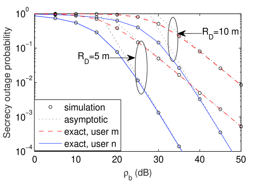
Figure 3: The SOP versus $\rho_{b}$, with $\rho_{e}=10$ dB, $\alpha=4$, $\lambda_{e}=10^{-3}$, $M=2$, $m=1$, $n=2$, and $r_{p}=10$ m. The exact analytical results are calculated from (2) and (1). The asymptotic analytical results are calculated from (22) and (25).

Fig. 3 plots the SOP of a single user ($m$-th and $n$-th) versus $\rho_{b}$ for different user zone radii. The curves represent the exact analytical SOP of both the $m$-th user and of $n$-th user derived in (2) and (1), respectively. The asymptotic analytical SOP of both the $m$-th and $n$-th users, are derived in (25) and (22), respectively. Fig. 3 confirms the close agreement between the simulation and analytical results. A specific observation is that the reduced SOP can be achieved by reducing the radius of the user zone, since a smaller user zone leads to a lower path-loss. Another observation is that the $n$-th user has a more steep slope than the $m$-th user. This is due to the fact that we have $m<n$ and the $m$-th user as well as $n$-th user achieve a secrecy diversity order of $m$ and $n$ respectively, as inferred from (25) and (22).

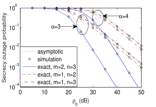
Figure 4: The SOP of user pair versus $\rho_{b}$, with $\rho_{e}=10$ dB, $\lambda_{e}=10^{-3}$, $R_{D}=10$ m, $M=3$, and $r_{p}=10$ m. The exact analytical results are calculated from (20). The asymptotic analytical results are calculated from (29).

Fig. 4 plots the SOP of the selected user pair versus the transmit SNR $\rho_{b}$ for different path-loss factors. The exact analytical SOP curves are plotted from (20). The asymptotic analytical SOP curves are plotted from (29). It can be observed that the two kinds of dashed curves have the same slopes. By contrast, the solid curves indicate a higher secrecy outage slope, which is due to the fact that the secrecy diversity order of the user pair is determined by that of the poor one. This phenomenon is also confirmed by the insights in Remark 1.

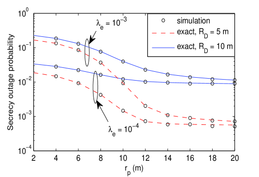
Figure 5: The SOP of user pair versus $r_{p}$, with $\rho_{b}=50$ dB, $\rho_{e}=40$ dB, $M=2$, $m=1$, $n=2$, and $\alpha=4$. The exact analytical results are calculated from (20).

Fig. 5 plots the SOP of the selected user pair versus $r_{p}$ for different densities of the Eves. We can observe that as expected, the SOP decreases, as the radius of the Eve-exclusion zone increases. Another option for enhancing the PLS is to reduce the radius of the user zone, since it reduces the total path loss. It is also worth noting that having a lower E density $\lambda_{e}$ results in an improved PLS, i.e. reduced SOP. This behavior is due to the plausible fact that a lower $\lambda_{e}$ results in having less Eves, which degrades the multiuser diversity gain, when the most detrimental E is selected. As a result, the destructive capability of the most detrimental E is reduced and hence the SOP is improved. It is worth pointing out that dynamic power sharing between two users is capable of improving the secrecy performance of the scenarios considered, but this is beyond the scope of this paper.

IV-B Secrecy outage probability with artificial noise

From Fig. 6 to Fig. 10, we investigate the secrecy performance in the presence of AN, which correspond to the scenario considered in Section III.

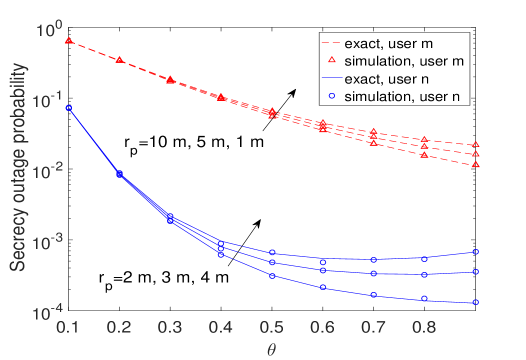
Figure 6: The SOP versus $\theta$, with $\alpha=4$, $R_{D_{1}}=5$ m, $R_{D_{2}}=10$ m, $\lambda_{e}=10^{-4}$, $N_{A}=4$, $\rho_{t}=30$ dB. The exact analytical results are calculated from  (4) and (3).

Fig. 6 plots the SOP of user $m$ and user $n$ versus $\theta$ for different Eve-exclusion zones. The solid and dashed curves represent the analytical performance of user $m$ and user $n$, corresponding to the results derived in (4) and (3). Monte Carlo simulations are used for verifying our derivations. Fig. 6 confirms a close agreement between the simulation and analytical results. Again, a reduced SOP can be achieved by increasing the Eve-exclusion zone, which degrades the channel conditions of the Eves. Another observation is that user $n$ achieves a lower SOP than user $m$, which is explained as follows: 1) user $n$ has better channel conditions than user $m$, owing to its lower path loss; and 2) user $n$ is capable of cancelling the interference imposed by user $m$ using SIC techniques, while user $m$ suffers from the interference inflicted by user $n$. It is also worth noting that the SOP is not a monotonic function of $\theta$. This phenomenon indicates that there exists an optimal value for power allocation, which depends on the system parameters.

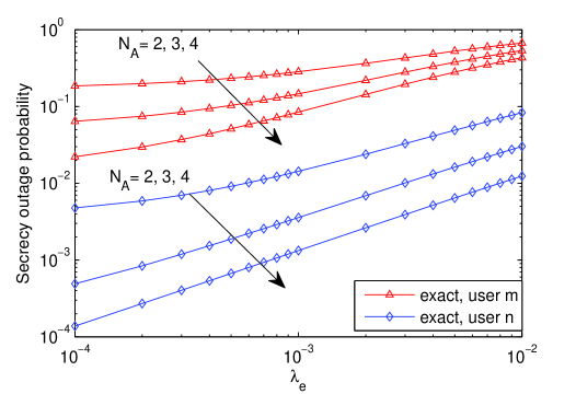
Figure 7: The SOP versus $\lambda_{e}$, with $\theta=0.8$, $\alpha=4$, $R_{D_{1}}=5$ m, $R_{D_{2}}=10$ m, $\rho_{t}=30$ dB, $r_{p}=4$ m. The exact analytical results are calculated from  (4) and (3).

Fig. 7 plots the SOP of user $m$ and user $n$ versus $\lambda_{e}$ for different number of antennas. We can observe that the SOP decreases, as the E density is reduced. This behavior is caused by the fact that a lower $\lambda_{e}$ leads to having less Eves, which reduces the multiuser diversity gain, when the most detrimental E is considered. As a result, the distinctive capability of the most detrimental E is reduced and hence the secrecy performance is improved. It is also worth noting that increasing the number of antennas is capable of increasing the secrecy performance. This is due to the fact that ${{\left\|{{{\bf{h}}_{m}}}\right\|}^{2}}$ in (32) and ${{\left\|{{{\bf{h}}_{n}}}\right\|}^{2}}$ in (34) both follow $Gamma\left({{N_{A}},1}\right)$ distributions, which is the benefit of the improved multi-antenna diversity gain.

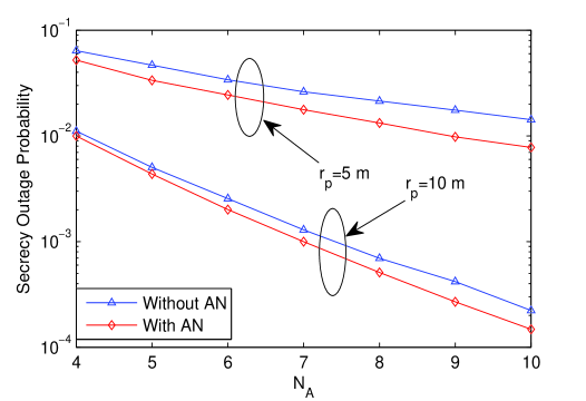
Figure 8: The SOP of the user pair versus $N_{A}$, with $R_{D_{1}}=5$ m, $R_{D_{2}}=10$ m, $\alpha=3$, $\lambda_{e}=10^{-3}$, $\rho_{t}=30$ dB.

Fig. 8 plots the SOP of the selected user pair versus $N_{A}$ for different path loss exponents. In this figure, the curves representing the case without AN are generated by setting $\theta=1$, which means that all the power is allocated to the desired signal. In this case, the BS only uses beamforming for transmitting the desired signals and no AN is generated. The curves in the presence of AN are generated by setting $\theta=0.9$. We show that the PLS can be enhanced by using AN. This behavior is caused by the fact that at the receiver side, user $m$ and user $n$ are only affected by the AN generated by each other; By contrast, the Eves are affected by the AN of both user $m$ and user $n$. We can observe that the SOP of the selected user pair decreases, as the Eve-exclusion radius increases.

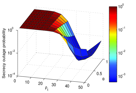
Figure 9: SOP of the user pair versus $\rho_{t}$ and $\theta$, with $N_{A}=4$, $\alpha=4$, $R_{D_{1}}=5$ m, $R_{D_{2}}=10$ m, $\lambda_{e}=10^{-4}$, $r_{p}=10$ m. The exact analytical results are calculated from  (42).

Fig. 9 plots the SOP of the selected user pair versus $\rho_{t}$ and $\theta$. It is observed that the SOP first decreases then increases as $\rho_{t}$ increases, which is in contrast to the traditional trend, where the SOP always decreases as the transmit SNR increases. This behavior can be explained as follows. The SOP of the selected user pair is determined by user $m$. As $\rho_{t}$ increases, on the one hand, the signal power of user $m$ is increased, which improves the secrecy performance; On the other hand, user $m$ also suffers from the interference imposed by user $n$ (including both the signal and AN), because when $\rho_{t}$ increases, the signal power of user $n$ is also increased, which in turn degrades the secrecy performance. As a consequence, there is a tradeoff between $\rho_{t}$ and the SOP. It is also noted that the power sharing factor $\theta$ also affect the optimal SOP associated with different values of $\rho_{t}$. This phenomenon indicates that it is of salient significance to select beneficial system parameters. Furthermore, optimizing the parameters $\rho_{t}$ and $\theta$ is capable of further improving the SOP.

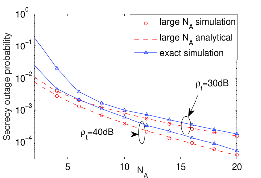
Figure 10: Large analysis for the SOP of user pair versus $N_{A}$, with $\theta=0.8$, $R_{D_{1}}=5$ m, $R_{D_{2}}=10$ m, $\lambda_{e}=10^{-4}$, $r_{p}=5$ m. The asymptotic analytical results are calculated from  (58).

Fig. 10 plots the SOP of large antenna arrays of the selected user pair versus $N_{A}$ parameterized by different transmit SNRs. The dashed curves represent the analytical SOP of the selected user pair, corresponding to the results derived in (58). We observe a close agreement between the theoretical analysis and the Monte Carlo simulations, which verifies the accuracy of our derivations. We observe that as $N_{A}$ increases, the approximation used in our analysis approaches the exact SOP. This phenomenon indicates that the asymptotic SOP derived converges to the exact values, when ${N_{A}}$ is a sufficiently large number.

V Conclusions

In this paper, the secrecy performance of applying the NOMA protocol in large-scale networks was examined. Specifically, stochastic geometry based techniques were used for modeling both the locations of NOMA users and of the Eves in the networks considered. Additionally, new analytical SOP expressions were derived for characterizing the system’s secrecy performance in both single-antenna and multiple-antenna scenarios. For the single-antenna scenario, the secrecy diversity order of the user pair was also characterized. It was analytically demonstrated that the secrecy diversity order was determined by that one of the user pair who had a poorer channel. For the multiple-antenna scenario, it was shown that the Eves’ channel quality is independent of the number of antennas at the BS for large antenna array scenarios. Numerical results were also presented for validating the analysis. It was concluded that the secrecy performance can be improved both by extending the Eve-exclusion zone and by generating AN at the BS. Assuming perfect SIC operations may lead to overestimating the performance of the networks considered, hence our future research may consider investigating imperfect SIC. Optimizing the power sharing between two NOMA users is capable of further improving the secrecy performance of the networks considered, which is another promising future research direction.

Appendix A: Proof of Lemma 1

To derive the CDF of ${F_{{\gamma_{B}}}}$, based on (2), we can formulate

$${F_{{\gamma_{B}}}}\left(x\right)=\Pr\left\{{\rho_{b}{a_{n}}{{\left|{{h_{n}}}\right|}^{2}}\leq x}\right\}={F_{{{\left|{{h_{n}}}\right|}^{2}}}}\left({\frac{x}{{\rho_{b}{a_{n}}}}}\right),$$ (A.1)

where ${F_{{{\left|{{h_{n}}}\right|}^{2}}}}$ is the CDF of the ordered channel gain for the $n$-th user. Assuming $y=\frac{x}{{\rho_{b}{a_{n}}}}$, and using order statistics [47] as well as applying binary series expansion, the CDF of the ordered channels has a relationship with the unordered channels captured as follows:

$${F_{{{\left|{{h_{n}}}\right|}^{2}}}}\left(y\right)={\varphi_{n}}\sum\limits_{p=0}^{M-n}{M-n\choose p}\frac{{{{\left({-1}\right)}^{p}}}}{{n+p}}{\left({{F_{{{\left|{{{\tilde{h}}_{n}}}\right|}^{2}}}}\left(y\right)}\right)^{n+p}},$$ (A.2)

where ${{F_{{{\left|{{{\tilde{h}}_{n}}}\right|}^{2}}}}}$ is the CDF of unordered channel gain for the $n$-th user.

Based on the assumption of homogeneous PPP, and by relying on polar coordinates, ${{F_{{{\left|{{{\tilde{h}}_{n}}}\right|}^{2}}}}}$ is expressed as

$${F_{{{\left|{{{\tilde{h}}_{n}}}\right|}^{2}}}}\left(y\right)=\frac{2}{{R_{D}^{2}}}\int_{0}^{{R_{D}}}{\left({1-{e^{-\left({1+{r^{\alpha}}}\right)y}}}\right)rdr}.$$ (A.3)

However, it is challenging to arrive at an easily implemented insightful expression for ${F_{{{\left|{{{\tilde{h}}_{n}}}\right|}^{2}}}}\left(y\right)$. Therefore, the Gaussian-Chebyshev quadrature relationship [48] is invoked for finding an approximation of (A.3) in the following form:

$${F_{{{\left|{{{\tilde{h}}_{n}}}\right|}^{2}}}}\left(y\right)\approx\sum\limits_{k=0}^{K}{{b_{k}}{e^{-{c_{k}}y}}}.$$ (A.4)

Substituting (A.4) into (A.2) and applying the multinomial theorem, the CDF ${F_{{{\left|{{h_{n}}}\right|}^{2}}}}$ of ordered channel gain is given by

$${F_{{{\left|{{h_{n}}}\right|}^{2}}}}\left(y\right)\approx{\varphi_{n}}\sum\limits_{p=0}^{M-n}{M-n\choose p}\frac{{{{\left({-1}\right)}^{p}}}}{{n+p}}$$

$$\times{\sum_{\tilde{S}_{n}^{p}}}{{n+p\choose{q_{0}}+\cdots+{q_{K}}}\left({\prod\limits_{k=0}^{K}{b_{k}^{{q_{k}}}}}\right){e^{-\sum\limits_{k=0}^{K}{{q_{k}}{c_{k}}y}}}}.$$ (A.5)

Substituting $y=\frac{x}{{\rho_{b}{a_{n}}}}$ into (Appendix A: Proof of Lemma 1), we can obtain (1). The proof is completed.

Appendix B: Proof of Lemma 4

Based on (34), we express the CDF of $F_{{B_{n}}}^{AN}$ as follows:

$$F_{{B_{n}}}^{AN}\left(x\right)=\Pr\left\{{{{\left\|{{{\bf{h}}_{n}}}\right\|}^{2}}\leq x\vartheta\left({\frac{{{P_{A}}}}{{{N_{A}}-1}}{Y_{n}}+\frac{{1+d_{n}^{\alpha}}}{{{a_{m}}}}}\right)}\right\}$$

$$=1-\sum\limits_{p=0}^{{N_{A}}-1}{\frac{{{\vartheta^{p}}{x^{p}}}}{{p!}}}\sum\limits_{q=0}^{p}{p\choose q}{Q_{3}}$$

$$\times\int\limits_{{D_{1}}}{{e^{-\frac{{\vartheta x}}{{{a_{m}}}}\left({1+d_{n}^{\alpha}}\right)}}{{\left({\frac{1}{{{a_{m}}}}\left({1+d_{n}^{\alpha}}\right)}\right)}^{p-q}}{f_{{D_{1}}}}\left({{\omega_{n}}}\right)d{\omega_{n}}},$$ (B.1)

where $\vartheta=\frac{{{a_{m}}}}{{{a_{n}}{P_{S}}}}$, ${Q_{3}}=\int_{0}^{\infty}{{e^{-\vartheta x{z_{n}}}}z_{n}^{q}}{f_{I_{n}^{AN}}}\left({{z_{n}}}\right)d{z_{n}}$, ${f_{I_{n}^{AN}}}$ and ${f_{{D_{1}}}}\left({{\omega_{n}}}\right)$ are the PDF of $I_{n}^{AN}$ and $D_{1}$. Here $I_{n}^{AN}=\frac{{{P_{A}}}}{{{N_{A}}-1}}{Y_{n}},{Y_{n}}={\left\|{{{\bf{h}}_{n}}{{\bf{V}}_{m}}}\right\|^{2}}$, and ${f_{{D_{1}}}}\left({{\omega_{n}}}\right)=\frac{1}{{\pi R_{{D_{1}}}^{2}}}$. Upon changing to polar coordinates and applying [35, Eq. (3.381.8)], we arrive at

$$F_{{B_{n}}}^{AN}\left(x\right)= 1-\frac{{\delta{e^{-\frac{{\vartheta x}}{{{a_{m}}}}}}}}{{R_{{D_{1}}}^{2}}}\sum\limits_{p=0}^{{N_{A}}-1}{\frac{{{\vartheta^{p}}{x^{p}}}}{{p!}}}\sum\limits_{q=0}^{p}{p\choose q}{Q_{3}}a_{m}^{q-p}$$

$$\times\sum\limits_{u=0}^{p-q}{p-q\choose u}\frac{{\gamma\left({u+\delta,\frac{{\vartheta x}}{{{a_{m}}}}R_{{D_{1}}}^{\alpha}}\right)}}{{{{\left({\frac{{\vartheta x}}{{{a_{m}}}}}\right)}^{u+\delta}}}}.$$ (B.2)

Finally we turn our attention on $Q_{3}$. It is readily seen that $I_{n}^{AN}$ obeys the Gamma distribution in conjunction with the parameter $\left({{N_{A}}-1,{\frac{{{P_{A}}}}{{{N_{A}}-1}}}}\right)$. Then we can obtain the PDF of ${f_{I_{n}^{AN}}}\left({{z_{n}}}\right)=\frac{{z_{n}^{{N_{A}}-2}{e^{-\frac{{{z_{n}}\left({{N_{A}}-1}\right)}}{{{P_{A}}}}}}}}{{{{\left({\frac{{{P_{A}}}}{{{N_{A}}-1}}}\right)}^{{N_{A}}-1}}\Gamma\left({{N_{A}}-1}\right)}}$. Applying [35, Eq. (3.326.2)], we can express $Q_{3}$ as ${Q_{3}}=\frac{{\Gamma\left({{N_{A}}-1+q}\right)}}{{\Gamma\left({{N_{A}}-1}\right){{\left({\frac{{{P_{A}}}}{{{N_{A}}-1}}}\right)}^{{N_{A}}-1}}{{\left({\vartheta x+\frac{{{N_{A}}-1}}{{{P_{A}}}}}\right)}^{{N_{A}}-1+q}}}}$. Upon substituting $Q_{3}$ into (Appendix B: Proof of Lemma 4), we obtain the CDF of $F_{{B_{n}}}^{AN}\left(x\right)$ as (4).

Appendix C: Proof of Lemma 5

Based on (32), we express the CDF of $F_{{B_{m}}}^{AN}$ as

$$F_{{B_{m}}}^{AN}\left(x\right)=\Pr\left\{{\gamma_{{B_{m}}}^{AN}\leq x}\right\}$$

$$=\Pr\left\{{\frac{{{a_{m}}\sigma_{s}^{2}{{\left\|{{{\bf{h}}_{m}}}\right\|}^{2}}}}{{{a_{n}}\sigma_{s}^{2}{{\left|{{{\bf{h}}_{m}}\frac{{{\bf{h}}_{n}^{\dagger}}}{{\left\|{{{\bf{h}}_{n}}}\right\|}}}\right|}^{2}}+{a_{n}}\sigma_{a}^{2}{{\left\|{{{\bf{h}}_{m}}{{\bf{V}}_{n}}}\right\|}^{2}}+1+d_{m}^{\alpha}}}\leq x}\right\}.$$ (C.1)

It may be readily seen that ${{{\left\|{{{\bf{h}}_{m}}}\right\|}^{2}}}$ obeys a Gamma distribution having the parameters of $\left({{N_{A}},1}\right)$. Hence the CDF of ${{{\left\|{{{\bf{h}}_{m}}}\right\|}^{2}}}$ is given by

$$F_{{B_{m}}}^{AN}\left(x\right)=1-{e^{-x}}\sum\limits_{p=0}^{{N_{A}}-1}{\frac{{{x^{p}}}}{{p!}}}.$$ (C.2)

Denoting ${X_{m}}={\left|{{{\bf{h}}_{m}}\frac{{{\bf{h}}_{n}^{\dagger}}}{{\left\|{{{\bf{h}}_{n}}}\right\|}}}\right|^{2}},{Y_{m}}={\left\|{{{\bf{h}}_{m}}{{\bf{V}}_{n}}}\right\|^{2}}$, based on (C.2), we can re-write (Appendix C: Proof of Lemma 5) as

$$F_{{B_{m}}}^{AN}\left(x\right)=\Pr\left\{{{{\left\|{{{\bf{h}}_{m}}}\right\|}^{2}}\leq x\nu\left({I_{m}^{AN}+\frac{{1+d_{m}^{\alpha}}}{{{a_{n}}}}}\right)}\right\}$$

$$=1-\int\limits_{{D_{2}}}{\int_{0}^{\infty}{\sum\limits_{p=0}^{{N_{A}}-1}{\frac{{{{\left({\nu x\left({{z_{m}}+\frac{{1+d_{m}^{\alpha}}}{{{a_{n}}}}}\right)}\right)}^{p}}}}{{p!}}}}}$$

$$\times\left({{e^{-\nu x{z_{m}}-\nu x\frac{{1+d_{m}^{\alpha}}}{{{a_{n}}}}}}}\right){f_{I_{m}^{AN}}}\left({{z_{m}}}\right){f_{{D_{2}}}}\left({{\omega_{m}}}\right)d{z_{m}}d{\omega_{m}},$$ (C.3)

where $\nu=\frac{{{a_{n}}}}{{{a_{m}}{P_{S}}}}$, ${f_{I_{m}^{AN}}}$ and ${{f_{{D_{2}}}}}$ are the PDF of $I_{m}^{AN}$ and ${{D_{2}}}$, respectively. Here we have $I_{m}^{AN}=\sigma_{s}^{2}{X_{m}}+\sigma_{a}^{2}{Y_{m}}$ and ${f_{{D_{2}}}}\left({{\omega_{m}}}\right)=\frac{1}{{\pi\left({R_{{D_{2}}}^{2}-R_{{D_{1}}}^{2}}\right)}}$. Applying a binary series expansion to (Appendix C: Proof of Lemma 5), we arrive at:

$$F_{{B_{m}}}^{AN}\left(x\right)=1-\sum\limits_{p=0}^{{N_{A}}-1}{\frac{{{\nu^{p}}{x^{p}}}}{{p!}}}\sum\limits_{q=0}^{p}{p\choose q}{Q_{1}}$$

$$\times\int\limits_{{D_{2}}}{{e^{-\nu x\frac{{1+d_{m}^{\alpha}}}{{{a_{n}}}}}}{{\left({\frac{{1+d_{m}^{\alpha}}}{{{a_{n}}}}}\right)}^{p-q}}{f_{{D_{2}}}}\left({{\omega_{m}}}\right)d{\omega_{m}}},$$ (C.4)

where ${Q_{1}}=\int_{0}^{\infty}{{e^{-\nu x{z_{m}}}}z_{m}^{q}}{f_{I_{m}^{AN}}}\left({{z_{m}}}\right)d{z_{m}}$. Note that the distance $d_{m}$ is determined by the location of $\omega_{m}$. Then we change to polar coordinates and applying a binary series expansion again, we obtain

$$F_{{B_{m}}}^{AN}\left(x\right)=1-\frac{{{2e^{-\frac{{\nu x}}{{{a_{n}}}}}}}}{{R_{{D_{2}}}^{2}-R_{{D_{1}}}^{2}}}\sum\limits_{p=0}^{{N_{A}}-1}{\frac{{{\nu^{p}}{x^{p}}}}{{p!}}}\sum\limits_{q=0}^{p}{p\choose q}$$

$$\times{Q_{1}}\frac{1}{{a_{n}^{p-q}}}\sum\limits_{u=0}^{p-q}{p-q\choose u}\int_{{R_{{D_{1}}}}}^{{R_{{D_{2}}}}}{{r^{u\alpha+1}}{e^{-\nu x{P_{S}}{r^{\alpha}}}}}dr.$$ (C.5)

By invoking [35, Eq. (3.381.8)], we obtain

$$F_{{B_{m}}}^{AN}\left(x\right)=1-\frac{{{2e^{-\frac{{\nu x}}{{{a_{n}}}}}}}}{{R_{{D_{2}}}^{2}-R_{{D_{1}}}^{2}}}\sum\limits_{p=0}^{{N_{A}}-1}{\frac{{{\nu^{p}}{x^{p}}}}{{p!}}}\sum\limits_{q=0}^{p}{p\choose q}{Q_{1}}\frac{1}{{a_{n}^{p-q}}}$$

$$\times\sum\limits_{u=0}^{p-q}{p-q\choose u}\frac{{\gamma\left({u+\delta,\frac{{\nu x}}{{{a_{n}}}}R_{{D_{2}}}^{\alpha}}\right)-\gamma\left({u+\delta,\frac{{\nu x}}{{{a_{n}}}}R_{{D_{1}}}^{\alpha}}\right)}}{{\alpha{{\left({\frac{{\nu x}}{{{a_{n}}}}}\right)}^{u+\delta}}}}.$$ (C.6)

Let us now turn our attention to the derivation of the integral $Q_{1}$ in (Appendix C: Proof of Lemma 5) – (Appendix C: Proof of Lemma 5). Note that $X_{m}$ follows the exponential distribution with unit mean, while $Y_{m}$ follows the distribution ${Y_{m}}\sim Gamma\left({{N_{A}}-1,1}\right)$. As such, the PDF of ${f_{I_{m}^{AN}}}$ is given by [25]

$${f_{I_{m}^{AN}}}\left({{z_{m}}}\right)=\left\{\begin{array}[]{l}\frac{{{t_{1}}}}{{{e^{\frac{{{z_{m}}}}{{{P_{S}}}}}}}}\left({1-\sum\limits_{l=0}^{{N_{A}}-2}{\frac{{{{\left({\frac{{{N_{A}}-1}}{{{P_{A}}}}-\frac{1}{{{P_{S}}}}}\right)}^{l}}z_{m}^{l}}}{{l!{e^{\left({\frac{{{N_{A}}-1}}{{{P_{A}}}}-\frac{1}{{{P_{S}}}}}\right){z_{m}}}}}}}}\right),\theta\neq\frac{1}{{{N_{A}}}}\\ \frac{{z_{m}^{{N_{A}}-1}{e^{-\frac{{{z_{m}}}}{{{P_{S}}}}}}}}{{{P_{S}}^{{N_{A}}}\left({{N_{A}}-1}\right)!}},\theta=\frac{1}{{{N_{A}}}}\\ \end{array}\right.,$$ (C.9)

where we have ${t_{1}}=\frac{{{{\left({1-\frac{{{P_{A}}}}{{\left({{N_{A}}-1}\right){P_{S}}}}}\right)}^{1-{N_{A}}}}}}{{{P_{S}}}}$. Based on (C.9), and applying [35, Eq. (3.326.2)], we can express $Q_{1}$ as follows:

$${Q_{1}}=\left\{\begin{array}[]{l}{\frac{{t_{1}}{\Gamma\left({q+1}\right)}}{{{{\left({x\nu+\frac{1}{{{P_{S}}}}}\right)}^{q+1}}}}-\sum\limits_{l=0}^{{N_{A}}-2}{\frac{{\frac{{t_{1}}}{{l!}}{{\left({\frac{{{N_{A}}-1}}{{{P_{A}}}}-\frac{1}{{{P_{S}}}}}\right)}^{l}}\Gamma\left({q+l+1}\right)}}{{{{\left({\nu x+\frac{{{N_{A}}-1}}{{{P_{A}}}}}\right)}^{q+l+1}}}}}},\theta\neq\frac{1}{{{N_{A}}}}\\ \frac{{\Gamma\left({q+{N_{A}}}\right)}}{{{P_{S}}^{{N_{A}}}\left({{N_{A}}-1}\right)!{{\left({\nu x+\frac{1}{{{P_{S}}}}}\right)}^{q+{N_{A}}}}}},\theta=\frac{1}{{{N_{A}}}}\\ \end{array}\right..$$ (C.12)

Upon substituting (C.12) into (Appendix C: Proof of Lemma 5), the CDF of $F_{{B_{m}}}^{AN}$ is given by (5).

Appendix D: Proof of Lemma 6

Based on (36), the CDF of ${F_{\gamma_{{E_{\kappa}}}^{AN}}}$ can be expressed as

$${F_{\gamma_{{E_{\kappa}}}^{AN}}}\left(x\right)=\Pr\left\{{\mathop{\max}\limits_{e\in{\Phi_{e}},{d_{e}}\geq{r_{p}}}\left\{{\frac{{{a_{\kappa}}{P_{S}}{X_{e,\kappa}}}}{{I_{e}^{AN}+d_{e}^{\alpha}}}}\right\}\leq x}\right\}$$

$$={E_{{\Phi_{e}}}}\left\{{\prod\limits_{e\in{\Phi_{e}},{d_{e}}\geq{r_{p}}}{\int_{0}^{\infty}{{F_{{X_{e,\kappa}}}}\left({\frac{{\left({z+d_{e}^{\alpha}}\right)x}}{{{a_{\kappa}}{P_{S}}}}}\right)}{f_{I_{e}^{AN}}}\left(z\right)dz}}\right\}.$$ (D.1)

Following a procedure similar to that used for obtaining (3), we apply the generating function and switch to polar coordinates. Then (Appendix D: Proof of Lemma 6) can be expressed as

$${F_{\gamma_{{E_{\kappa}}}^{AN}}}\left(x\right)=\exp\left[{-2\pi{\lambda_{e}}\int_{{r_{p}}}^{\infty}{r{e^{-\frac{x}{{{a_{\kappa}}{P_{S}}}}{r^{\alpha}}}}dr{Q_{2}}}}\right],$$ (D.2)

where ${Q_{2}}=\int_{0}^{\infty}{{e^{-z\frac{x}{{{a_{\kappa}}{P_{S}}}}}}}{f_{I_{e}^{AN}}}\left(z\right)dz$. Applying [35, Eq. (3.381.9)], we arrive at

$${F_{\gamma_{{E_{\kappa}}}^{AN}}}\left(x\right)=\exp\left[{-\frac{{\mu_{\kappa 1}^{AN}\Gamma\left({\delta,\mu_{\kappa 2}^{AN}x}\right)}}{{{x^{\delta}}}}{Q_{2}}}\right].$$ (D.3)

Let us now turn our attention to solving the integral $Q_{2}$. Note that all the elements of ${{{\bf{h}}_{e}}{{\bf{V}}_{m}}}$ and ${{{\bf{h}}_{e}}{{\bf{V}}_{n}}}$ are independent complex Gaussian distributed with a zero mean and unit variance. We introduce the notation ${Y_{e,m}}={\left\|{{{\bf{h}}_{e}}{{\bf{V}}_{m}}}\right\|^{2}}$ and ${Y_{e,n}}={\left\|{{{\bf{h}}_{e}}{{\bf{V}}_{n}}}\right\|^{2}}$. As a consequence, both ${Y_{e,m}}$ and ${Y_{e,n}}$ obey the $Gamma\left({{N_{A}}-1,1}\right)$ distribution. Based on the properties of the Gamma distribution, we have ${a_{m}}\sigma_{a}^{2}{Y_{e,m}}\sim Gamma\left({{N_{A}}-1,{a_{m}}\sigma_{a}^{2}}\right),{a_{n}}\sigma_{a}^{2}{Y_{e,n}}\sim Gamma\left({{N_{A}}-1,{a_{n}}\sigma_{a}^{2}}\right)$. Then the sum of these two items $I_{e}^{AN}$ obeys the generalized integer Gamma (GIG) distribution. According to [49], the PDF of $I_{e}^{AN}$ is given by

$${f_{I_{e}^{AN}}}\left(z\right)= {\left({-1}\right)^{{N_{A}}-1}}\prod\limits_{i=1}^{2}{\tau_{i}^{{N_{A}}-1}}\sum\limits_{i=1}^{2}{\sum\limits_{j=1}^{{N_{A}}-1}{}}$$

$$\frac{{{a_{{N_{A}}-j,{N_{A}}-1}}}}{{\left({j-1}\right)!}}{\left({2{\tau_{i}}-L}\right)^{j-\left({2{N_{A}}-2}\right)}}{z^{j-1}}{e^{-{\tau_{i}}z}}.$$ (D.4)

Upon substituting (Appendix D: Proof of Lemma 6) into (D.3), as well as applying [35, Eq. (3.381.4)], after some further manipulations, we obtain the CDF of ${F_{\gamma_{{E_{\kappa}}}^{AN}}}$ as

$${F_{\gamma_{{E_{\kappa}}}^{AN}}}\left(x\right)=\exp\left[{\Omega\frac{{\Gamma\left({\delta,x\mu_{\kappa 2}^{AN}}\right)}}{{\sum\limits_{p=0}^{j}{j\choose p}{{{{\left(x\right)}^{p+\delta}}{{\left({{a_{\kappa}}{P_{S}}}\right)}^{-p}}}}\tau_{i}^{j-p}}}}\right].$$ (D.5)

Upon setting the derivative of the CDF in (D.5), we can obtain (6).

References

• [1] Z. Qin, Y. Liu, Z. Ding, Y. Gao, and M. Elkashlan, “Physical layer security for 5G non-orthogonal multiple access in large-scale networks,” in Proc. of International Commun. Conf. (ICC), May 2016, pp. 1–6.
• [2] P. Wang, J. Xiao, and L. P, “Comparison of orthogonal and non-orthogonal approaches to future wireless cellular systems,” vol. 1, no. 3, pp. 4–11, Sep. 2006.
• [3] L. Dai, B. Wang, Y. Yuan, S. Han, C. l. I, and Z. Wang, “Non-orthogonal multiple access for 5G: solutions, challenges, opportunities, and future research trends,” IEEE Commun. Mag., vol. 53, no. 9, pp. 74–81, Sep. 2015.
• [4] 3rd Generation Partnership Project (3GPP), “Study on downlink multiuser superposition transmission for LTE,” Mar. 2015.
• [5] Y. Saito, Y. Kishiyama, A. Benjebbour, T. Nakamura, A. Li, and K. Higuchi, “Non-orthogonal multiple access (NOMA) for cellular future radio access,” in Proc. Vehicular Technology Conference (VTC Spring), June Dresden, Germany, Jun. 2013, pp. 1–5.
• [6] Z. Ding, Y. Liu, J. Choi, Q. Sun, M. Elkashlan, C.-L. I, and H. V. Poor, “Application of non-orthogonal multiple access in LTE and 5G networks,” IEEE Commun. Mag., Feb. 2017.
• [7] T. M. Cover, “Broadcast channels,” IEEE Trans. Inf. Theory, vol. 18, no. 1, pp. 2–14, 1972.
• [8] J. G. Andrews, “Interference cancellation for cellular systems: a contemporary overview,” IEEE Trans. Wireless Commun., vol. 12, no. 2, pp. 19–29, Apr. 2005.
• [9] Z. Ding, Z. Yang, P. Fan, and H. V. Poor, “On the performance of non-orthogonal multiple access in 5G systems with randomly deployed users,” IEEE Signal Process. Lett., vol. 21, no. 12, pp. 1501–1505, 2014.
• [10] S. Timotheou and I. Krikidis, “Fairness for non-orthogonal multiple access in 5G systems,” IEEE Signal Process. Lett., vol. 22, no. 10, pp. 1647–1651, Oct 2015.
• [11] Y. Liu, Z. Ding, M. Elkashlan, and H. V. Poor, “Cooperative non-orthogonal multiple access with simultaneous wireless information and power transfer,” IEEE J. Sel. Areas Commun., vol. 34, no. 4, April 2016.
• [12] J. Choi, “Minimum power multicast beamforming with superposition coding for multiresolution broadcast and application to NOMA systems,” IEEE Trans. Commun., vol. 63, no. 3, pp. 791–800, March 2015.
• [13] Q. Sun, S. Han, C.-L. I, and Z. Pan, “On the ergodic capacity of MIMO NOMA systems,” IEEE Wireless Commun. Lett., vol. 4, no. 4, pp. 405–408, Aug. 2015.
• [14] Y. Zhang, H. M. Wang, T. X. Zheng, and Q. Yang, “Energy-efficient transmission design in non-orthogonal multiple access,” IEEE Trans. Veh. Technol., to appear in 2016.
• [15] Y. Liu, Z. Qin, M. Elkashlan, Y. Gao, and N. Arumugam, “Non-orthogonal multiple access in massive MIMO aided heterogeneous networks,” in Proc. of Global Commun. Conf. (GLOBECOM), Washington D.C, USA, Jun. 2016.
• [16] A. D. Wyner, “The wire-tap channel,” Bell Syst. Tech. J., vol. 54, no. 8, pp. 1355–1387, 1975.
• [17] A. Mukherjee and A. Swindlehurst, “Robust beamforming for security in MIMO wiretap channels with imperfect CSI,” IEEE Trans. Signal Process., vol. 59, no. 1, pp. 351–361, Jan. 2011.
• [18] Z. Ding, K. K. Leung, D. L. Goeckel, and D. Towsley, “On the application of cooperative transmission to secrecy communications,” IEEE J. Sel. Areas Commun., vol. 30, no. 2, pp. 359–368, Feb. 2012.
• [19] Y. Liu, L. Wang, T. T. Duy, M. Elkashlan, and T. Duong, “Relay selection for security enhancement in cognitive relay networks,” IEEE Wireless Commun. Lett., vol. 4, no. 1, pp. 46–49, Feb. 2015.
• [20] Y. Zou, X. Wang, W. Shen, and L. Hanzo, “Security versus reliability analysis of opportunistic relaying,” IEEE Trans. Veh. Technol., vol. 63, no. 6, pp. 2653–2661, Jul. 2014.
• [21] Y. Liu, L. Wang, S. Zaidi, M. Elkashlan, and T. Duong, “Secure D2D communication in large-scale cognitive cellular networks: A wireless power transfer model,” IEEE Trans. Commun., vol. 64, no. 1, pp. 329–342, Jan 2016.
• [22] E. Tekin and A. Yener, “The general Gaussian multiple-access and two-way wiretap channels: Achievable rates and cooperative jamming,” IEEE Trans. Inf. Theory, vol. 54, no. 6, pp. 2735–2751, Jun. 2008.
• [23] S. Goel and R. Negi, “Guaranteeing secrecy using artificial noise,” IEEE Trans. Wireless Commun., vol. 7, no. 6, pp. 2180–2189, Jun. 2008.
• [24] X. Zhou and M. R. McKay, “Secure transmission with artificial noise over fading channels: Achievable rate and optimal power allocation,” IEEE Trans. Veh. Technol., vol. 59, no. 8, pp. 3831–3842, Oct. 2010.
• [25] X. Zhang, X. Zhou, and M. R. McKay, “Enhancing secrecy with multi-antenna transmission in wireless ad hoc networks,” IEEE Trans. Inf. Forensics Security, vol. 8, no. 11, pp. 1802–1814, Nov. 2013.
• [26] Y. Wu, R. Schober, D. W. K. Ng, C. Xiao, and G. Caire, “Secure massive MIMO transmission with an active eavesdropper,” IEEE Trans. Inf. Forensics Security, vol. 62, no. 7, pp. 3880–3900, July 2016.
• [27] Y. Zhang, H. M. Wang, Q. Yang, and Z. Ding, “Secrecy sum rate maximization in non-orthogonal multiple access,” IEEE Commun. Lett., vol. 20, no. 5, pp. 930–933, May 2016.
• [28] P. C. Pinto, J. Barros, and M. Z. Win, “Secure communication in stochastic wireless networks part I: Connectivity,” IEEE Trans. Inf. Forensics Security, vol. 7, no. 1, pp. 125–138, Feb. 2012.
• [29] N. Romero-Zurita, D. McLernon, M. Ghogho, and A. Swami, “PHY layer security based on protected zone and artificial noise,” IEEE Signal Process. Lett., vol. 20, no. 5, pp. 487–490, May 2013.
• [30] L. L. Hanzo, Y. Akhtman, L. Wang, and M. Jiang, MIMO-OFDM for LTE, WiFi and WiMAX: Coherent versus non-coherent and cooperative turbo transceivers, 2010, vol. 9.
• [31] L. L. Hanzo, T. Liew, B. Yeap, R. Tee, and S. X. Ng, Turbo coding, turbo equalisation and space-time coding: EXIT-chart-aided near-capacity designs for wireless channels, 2011.
• [32] O. O. Koyluoglu, C. E. Koksal, and H. E. Gamal, “On secrecy capacity scaling in wireless networks,” IEEE Trans. Inf. Theory, vol. 58, no. 5, pp. 3000–3015, May 2012.
• [33] Z. Qin, Y. Liu, Y. Gao, M. Elkashlan, and A. Nallanathan, “Wireless powered cognitive radio networks with compressive sensing and matrix completion,” IEEE Trans. Commun., 2016.
• [34] W. K. D. Stoyan and J. Mecke, Stochastic Geometry and its Applications, 2nd ed.   John Wiley and Sons, 1996.
• [35] I. S. Gradshteyn and I. M. Ryzhik, Table of Integrals, Series and Products, 6th ed.   New York, NY, USA: Academic Press, 2000.
• [36] M. Bloch, J. Barros, M. R. D. Rodrigues, and S. W. McLaughlin, “Wireless information-theoretic security,” IEEE Trans. Inf. Theory, vol. 54, no. 6, pp. 2515–2534, June 2008.
• [37] N. Yang, H. A. Suraweera, I. B. Collings, and C. Yuen, “Physical layer security of TAS/MRC with antenna correlation,” IEEE Trans. Inf. Forensics Security, vol. 8, no. 1, pp. 254–259, Jan. 2013.
• [38] L. Wang, N. Yang, M. Elkashlan, P. L. Yeoh, and J. Yuan, “Physical layer security of maximal ratio combining in two-wave with diffuse power fading channels,” IEEE Trans. Inf. Forensics Security, vol. 9, no. 2, pp. 247–258, Feb. 2014.
• [39] S. Goel and R. Negi, “Guaranteeing secrecy using artificial noise,” IEEE Trans. Wireless Commun., vol. 7, no. 6, pp. 2180–2189, June 2008.
• [40] Z. Ding, P. Fan, and H. V. Poor, “Impact of user pairing on 5G nonorthogonal multiple-access downlink transmissions,” IEEE Trans. Veh. Technol., vol. 65, no. 8, pp. 6010–6023, Aug. 2016.
• [41] R. Steele and L. Hanzo, Mobile Radio Communications: Second and Third Generation Cellular and WATM Systems: 2nd, 1999.
• [42] Y. Liu, M. Elkashlan, Z. Ding, and G. K. Karagiannidis, “Fairness of user clustering in MIMO non-orthogonal multiple access systems,” IEEE Commun. Lett., vol. 20, no. 7, pp. 1465–1468, July 2016.
• [43] Z. Ding, R. Schober, and H. V. Poor, “A general MIMO framework for NOMA downlink and uplink transmission based on signal alignment,” IEEE Trans. Wireless Commun., vol. 15, no. 6, pp. 4438–4454, June 2016.
• [44] H. Xie, B. Wang, F. Gao, and S. Jin, “A full-space spectrum-sharing strategy for massive MIMO cognitive radio systems,” IEEE J. Sel. Areas Commun., vol. 34, no. 10, pp. 2537–2549, Oct. 2016.
• [45] H. Xie, F. Gao, and S. Jin, “An overview of low-rank channel estimation for massive MIMO systems,” IEEE Access, vol. 4, pp. 7313–7321, 2016.
• [46] Z. Ding and H. V. Poor, “Design of Massive-MIMO-NOMA with limited feedback,” IEEE Signal Process. Lett., vol. 23, no. 5, pp. 629–633, May 2016.
• [47] H. A. David and N. Nagaraja, Order Statistics, 3rd ed.   John Wiley, 2003.
• [48] Y. Liu, Z. Ding, M. Elkashlan, and J. Yuan, “Nonorthogonal multiple access in large-scale underlay cognitive radio networks,” IEEE Trans. Veh. Technol., vol. 65, no. 12, pp. 10 152–10 157, Dec. 2016.
• [49] C. A. Coelho, “The generalized integer Gamma distribution a basis for distributions in multivariate statistics,” Journal of Multivariate Analysis, vol. 64, no. 1, pp. 86–102, 1998.