Unified Framework for the Effective Rate Analysis of Wireless Communication Systems over MISO Fading Channels

Abstract

This paper proposes a unified framework for the effective rate analysis over arbitrary correlated and not necessarily identical multiple inputs single output (MISO) fading channels, which uses moment generating function (MGF) based approach and H transform representation. The proposed framework has the potential to simplify the cumbersome analysis procedure compared to the probability density function (PDF) based approach. Moreover, the effective rates over two specific fading scenarios are investigated, namely independent but not necessarily identical distributed (i.n.i.d.) MISO hyper Fox’s H fading channels and arbitrary correlated generalized $K$ fading channels. The exact analytical representations for these two scenarios are also presented. By substituting corresponding parameters, the effective rates in various practical fading scenarios, such as Rayleigh, Nakagami-$m$, Weibull/Gamma and generalized $K$ fading channels, are readily available. In addition, asymptotic approximations are provided for the proposed H transform and MGF based approach as well as for the effective rate over i.n.i.d. MISO hyper Fox’s H fading channels. Simulations under various fading scenarios are also presented, which support the validity of the proposed method.

I Introduction

When evaluating the maximum achievable bit rate of a wireless system over fading channels, Shannon’s channel capacity is the most important performance metric. It has also been widely adopted as the basis of performance analysis as well as mechanism design. However, many emerging applications are real-time applications, for example voice over IP, interactive video and most of the smart grid applications. For these real-time applications, not only throughput, but also delay should be considered as one of the quality of service (QoS) requirements. Unfortunately, delay performance cannot be analysed using the traditional Shannon’s theory.

In order to deal with this issue, the theory of effective rate (or effective capacity) has been proposed by Wu and Negi [1], which bridges the gap between statistical QoS guarantees and the maximum achievable transmission rate. Since then it has been widely used as a powerful analytical tool and QoS provisioning metric in different scenarios. In [2], the resource allocation and flow selection algorithms for video distribution over wireless networks have been studied based on the effective rate theory, where energy efficiency and statistical delay bound have been considered. In [3] and [4], scheduling algorithms have been studied for the multi-user time division downlink systems, exploiting the effective rate as the key to characterizing QoS constraints. In [5], the effective rate of two-hop wireless communication systems has been studied, where the impact of nodes’ buffer constraints on the throughput has been considered. The effective rate has also been applied in the research of cognitive radio networks [6, 7] for assisting QoS analysis.

The channel’s fading effect is one major reason for the fluctuation of the instantaneous channel capacity, but how to analyse the effective rate under different fading scenarios is still an open research area. There exist a few successful attempts, such as the effective rate over Nakagami-$m$, Rician and generalized $K$ [8], Weibull [9], $\eta{-}\mu$ [10] , $\alpha{-}\mu$ [11], $\kappa{-}\mu$ shadowed channels [12], correlated exponential channels[13]. In [14], the effective rate over correlated Nakagami-$m$ channels has been obtained in closed form, where the effective rate over correlated Rician fading channel has also been derived in analytical form.

These approaches can be categorized as probability density function (PDF) based method, since the analyses highly rely on the exact or approximated PDF of the signal-to-noise ratio (SNR). A general PDF based framework for the multiple inputs single output (MISO) effective rate analysis has been proposed in [8]. However, the joint PDF is unavailable for many fading channels and it is often very hard, if not impossible, to obtain the exact PDF for further analysis. Hence many researches have put a lot of effort on approximating the PDF of multiple fading channels[8, 11, 12]. This fact results in the situation that the PDF based effective rate analyses are generally studied in a case-by-case way.

To address aforementioned issues, this paper proposes a moment generating function (MGF) based framework for the effective rate analysis over MISO fading channels using H transform representation. It has been clearly pointed out in [15, 16, 17] that MGF based approaches are beneficial in simplifying the analysis or even enabling the calculations of some important performance indexes when the PDF based approaches seem impractical. There are successful trials to use the MGF based approach to analyse the effective rate under single input single output (SISO) conditions[18] and multi-hop systems[19]. In addition, H transform analysis method [20] has been exploited in this paper. Besides effective rate, many important metrics in the wireless communication system, for example ergodic capacity, error probability and error exponents, are defined in integrations form. It can be observed from vast amount of literatures that it is non-trivial and usually complicated to deal with these integrations [8, 9, 10, 11, 12, 13, 14, 15], especially when multivariate random variable is involved. It has been pointed out in [20] that H transform is a potential unified analysis method, which can provide a systematic language in dealing with the statistical metrics involving random variables in the wireless communication systems. This aspect will be shown in later part of this paper.

The scope of this paper is effective rate over arbitrary correlated and not necessarily identical MISO fading channels. Note that when dealing with multiple channels, the instantaneous channel power gain at the receiver is described by multivariate random variable in general cases, which is different from the SISO conditions where univariate random variable may be sufficient. In [18], the SISO case is well studied, yet the results are hard to extend to multiple channel conditions, which is the main focus of this paper. Moreover, in this paper we use the H transform and multivariate Fox’s H function to present the effective rate over both i.n.i.d. and correlated fading channels, which further simplify the analysis and provide a more general analytical framework. The major contributions of this paper are listed as follows:

• A MGF based framework is proposed for analysing the effective rate over arbitrary correlated and not necessarily identical MISO fading channels using H transform representation. Due to the properties of H transform, the cumbersome mathematical calculation involving integration operation can be simplified.

• H transform involving multivariate Fox’s H function is investigated. As many important metrics in wireless communication systems can be represented by H transform and the statistical properties of multiple fading channels may be characterized using multivariate Fox’s H functions, the obtained results are also valuable in the analysis of other metrics in the multiple channel conditions. Also to the authors’ best knowledge, this work is the first to deal with multiple channel problems within the H transform framework.

• Effective rate over both i.n.i.d. and correlated channel scenarios are studied. The exact analytical expressions of effective rate over i.n.i.d. MISO hyper Fox’s H fading channels and arbitrary correlated generalized $K$ fading channels are given. The effective rates over various practical fading channels are readily available by simply substituting corresponding parameters, such as generalized $K$ and Weibull/Gamma fading channels, which avoids the case-by-case study in these fading scenarios.

• Asymptotic approximations are provided for the effective rate analysis over MISO fading channels, where the truncation error and the discretization error are studied. Using this approximation, the proposed effective rate expressions over i.n.i.d. MISO hyper Fox’s H fading channels can be accurately estimated in a unified and closed-form framework.

The rest of this paper is organized as follows. System model is introduced in Section II. Section III proposes the MGF based approach for MISO effective rate over arbitrary correlated and not necessarily identical fading channels using H transform representation. The effective rate over i.n.i.d. MISO hyper Fox’s H fading channel as well as arbitrary correlated generalized $K$ fading channels is investigated in Section IV, where several special cases are discussed. Then approximations are investigated in Section V, with simulation results presented in Section VI. Finally, conclusions are drawn in Section VII.

Throughout the paper, the following notations are used. $\mathbb{C}$ denotes complex numbers. Bold letters denote vectors. $\mathbf{1}_{N}$ denotes all-one vector of $N$ elements. $(\cdot)^{\dagger}$ denotes the Hermitian transpose. $\mathbb{E}\{\cdot\}$ denotes the expectation operator of a random variable and $\text{Pr}\{\cdot\}$ is the probability function. $\Gamma(z)$ is the gamma function [21, eq.(5.2.1)]. $H^{m{,}n}_{p{,}q}\left[\cdot\right]$ and $H\left[\cdot\right]$ denote the univariate Fox’s H function or multivariate Fox’s H function defined by (33)-(39) depending on the variates involved, which are detailed in Appendix -A. $\mathbb{H}\{\cdot\}(\cdot)$ denotes the Fox’s H transform. A bold dash “—” is used where no parameter is present. $f(\gamma)$ denotes PDF function, while $\phi(s)$ denotes MGF function. Some frequently used parameter sequences have been summarized in Table I.

TABLE I: Frequently Used Order and Parameter Sequences

Symbols	Order and Parameter Sequences
$\mathbf{O}_{\text{MGF}}$ $\mathbf{P}_{\text{MGF}}$	$(1,0,0,1)$ $(1,1,\textbf{---},0,\textbf{---},1)$
$\mathbf{O}_{\text{ER}}$ $\mathbf{P}_{\text{ER}}$	$(1,0,0,1)$ $(1,1,\textbf{---},A-1,\textbf{---},1)$
$\mathbf{O}_{f}$ $\mathbf{P}_{f}$	$(m,n,p,q)$ $(u,v,\mathbf{c},\mathbf{d},\mathbf{C},\mathbf{D})$
$\mathbf{O}_{\phi}$ $\mathbf{P}_{\phi}$	$(n+1,m,q,p+1)$ $(u/v,1/v,1-\mathbf{d}-\mathbf{D},(0,1-\mathbf{c}-\mathbf{C}),\mathbf{D},(1,\mathbf{C}))$

II System Model

In this paper, a MISO fading channel model is considered, where there are $N$ transmit antennas and only one receive antenna as shown in Fig. 1. The channels are assumed to be flat block fading, then the channel input-output relation can be written as

$$y=\mathbf{hx}+n_{{}_{0}},$$ (1)

where $\mathbf{h}\in{\mathbb{C}}^{1\times N}$ denotes the MISO channel vector, $\mathbf{x}$ is the transmit signal vector, and $n_{{}_{0}}$ represents the complex additive white Gaussian noise with zero mean and variance $N_{0}$. It is assumed that the transmission power is uniformly allocated across the transmit antennas, and the channels are assumed to be arbitrarily correlated and not necessarily identically distributed.

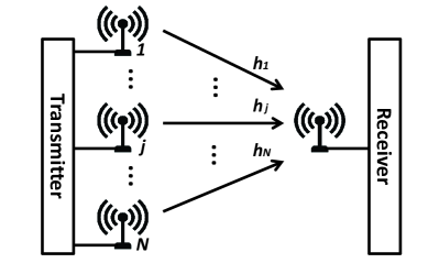
Figure 1: MISO system model.

The average transmit SNR is defined as $\rho=\frac{P}{BN_{0}}$, where $P$ is the average transmit power of the system and $B$ denotes the bandwidth. The channel state information is assumed to be only available at the receiver and the instantaneous channel power gain of the $j$th channel is defined by $\gamma_{j}=|h_{j}|^{2}$, where $h_{j}$ is the $j$th component of the fading vector $\mathbf{h}$. In this paper, we consider the maximum ratio transmission scheme, hence the instantaneous channel power gain at the receiver end can be defined by $\gamma_{\text{end}}{=}\sum_{j{=}1}^{N}\gamma_{j}$. The joint MGF $\phi_{\text{end}}$ is defined by $\phi_{\text{end}}(s)=\mathbb{E}\{e^{-s\sum_{j=1}^{N}\gamma_{j}}\}$. Specifically, if the channels are independent with each other, then the joint MGF $\phi_{{\text{end}}}(s)$ can be expressed by the product of the MGF of individual channel’s power gain as

$$\phi_{\text{end}}(s)=\prod_{j{=}1}^{N}\phi_{j}(s),$$ (2)

where $\phi_{j}(s)$ is defined by $\phi_{j}(s)=\int_{0}^{\infty}e^{-s\gamma}f_{j}(\gamma)d\gamma$ and $f_{j}(\gamma)$ is the PDF of the $j$th channel’s power gain.

III Effective Rate Analysis Using MGF

Effective rate is the maximum constant rate that a fading channel can support under statistical delay constraints, which can be written as [1]

$$R(\theta)=-\frac{1}{\theta T}\ln\mathbb{E}\left\{e^{-\theta TC}\right\},\quad\theta\neq 0,$$ (3)

where $C$ represents the system’s throughput during a single time block and $T$ denotes the duration of a time block. The QoS exponent $\theta$ is given by [1]

$$\theta=-\lim_{z\rightarrow\infty}\frac{\ln\text{Pr}\{L>z\}}{z},$$ (4)

where $L$ is the equilibrium queue-length of the buffer at the transmitter. When $z$ is large, the buffer violation probability can be approximated by $\text{Pr}\{L\geq z\}\approx e^{-\theta z}$. Correspondingly, if we denote the steady-state delay at the buffer by $D_{\text{delay}}$, then the probability of $D_{\text{delay}}$ exceeding the maximum allowed delay $d_{\text{max}}$ can be given by $\text{Pr}\{D_{\text{delay}}\geq d_{\text{max}}\}\approx e^{-\theta\delta d_{\text{max}}}$, where $\delta$ is determined by the characters of the queueing system [22]. Hence the minimum required QoS exponent $\theta_{0}$ is decided by the delay constraints, and in order to guarantee the delay performance, the QoS exponent $\theta$ has to satisfy the constraint $\theta\geq\theta_{0}$. Moreover, when $\theta_{0}\rightarrow 0$, the effective rate approaches the Shannon’s capacity [22].

When the transmitter sends uncorrelated circularly symmetric zero-mean complex Gaussian signals, the effective rate can be written as [22]

$$R(\theta){=}{-}\frac{1}{A}\log_{2}\mathbb{E}\left\{\left(1{+}\frac{\rho}{N}\gamma_{\text{end}}\right)^{{-}A}\right\},$$ (5)

where $A=\theta TB/\ln 2$. Normally, (5) will involve multiple integrations of multivariate functions, since the PDF of $\gamma_{\text{end}}=\sum_{j=1}^{N}\gamma_{j}$ is described by multivariate random variables in general cases. Yet by using the MGF instead of PDF and applying the H transform theory, the effective rate can be derived as follows.

Theorem 1:

The effective rate over arbitrary correlated and not necessarily identically distributed MISO fading channels can be given by

$$R(\theta){=} {-}\frac{1}{A}\log_{2}\frac{1}{\Gamma(A)}\mathbb{H}\left\{\phi_{\text{end}}(\frac{\rho s}{N}),\mathbf{O}_{\text{ER}},\mathbf{P}_{\text{ER}}\right\}\big{(}1\big{)},$$ (6)

$${\equiv} {-}\frac{1}{A}\log_{2}\frac{N}{\rho\Gamma(A)}\mathbb{H}\left\{\phi_{\text{end}}(s),\mathbf{O}_{\text{ER}},\mathbf{P}_{\text{ER}}\right\}\big{(}\frac{N}{\rho}\big{)},$$ (7)

where $\mathbf{O}_{\text{ER}}{=}(1,0,0,1)$ and $\mathbf{P}_{\text{ER}}{=}(1{,}{1}{,}{\textbf{---}}{,}A{-}1{,}{\textbf{---}}{,}1)$.

Proof.

See Appendix -B. ∎

Remark: The integral form of the effective rate of MISO fading channels can be obtained by using H transform definition and substituting the identity of $e^{{-}s}s^{A{-}1}=H^{1,0}_{0,1}\left[s\bigg{|}\begin{matrix}{\textbf{---}}\\ (A{-}1,1)\end{matrix}\right]$ [23, eq.(2.22)] into (6), which can be written as

$$R(\theta){=}{-}\frac{1}{A}\log_{2}\frac{1}{\Gamma(A)}\int_{0}^{\infty}e^{{-}s}s^{A{-}1}\phi_{\text{end}}(\frac{\rho s}{N})ds.$$ (8)

Using the fact that $0\leq\phi_{\text{end}}(s)\leq 1$, the integral can be proved to be absolutely converge. Hence the H transform in (6) and (7) exist.

We highlight that (6) and its equivalent (7) in H transform form are more attractive than the integral form in (8). On one hand, the MGF of most commonly used fading distributions can be written in Fox’s H function format[24], which facilitates the application of Theorem 1. On the other hand, we can interpret the effective rate as the H transform of the PDF or MGF of the power gain by the parameter sequence $\mathbf{O}_{\text{ER}}$ and $\mathbf{P}_{\text{ER}}$ with some more manipulations. It has been studied in [20] that many important metrics such as ergodic capacity, error probability, error exponent can be expressed in similar H transform format with corresponding parameter sequences. Note that one merit of H transform is that the manipulation of parameter sequences only involves very basic arithmetic operations, hence the H transform representation can provide a unified, systematic and simple framework for wireless performance analysis such as effective rate. In addition, in Section IV, we will show that for deriving MGF from the known PDF or analysing effective rate over SISO, i.n.i.d. and correlated scenarios, H transform is a very useful analysing tool.

In addition, compared to the PDF based approach, the MGF based approach has many advantages. First, the PDF based approach can be viewed as a special case of the MGF based approach. This is due to the fact that in the PDF based approach, the joint PDF has to be obtained in advance of further analysis. When the joint PDF is available, by using the relationship of PDF and MGF, it can be proved that the PDF based approach is involved in the case of $N=1$ in the proposed MGF based approach. Second, in the i.n.i.d. scenarios, the joint MGF can be calculated by the product of the individual channels’ MGF, which enables the analyses where the PDF based approach has difficulties [25, 11]. This feature makes the analysis more flexible and applicable to different and complex channel conditions.

IV Exact effective rate over MISO fading channels

In this section, we will investigate the effective rate over specific i.n.i.d. and correlated channels. For the i.n.i.d. scenario, the effective rate over i.n.i.d. hyper Fox’s H fading channels is derived, while the arbitrary correlated generalized $K$ fading channels are considered for the correlated scenario.

IV-A Effective rate over i.n.i.d. MISO hyper Fox’s H fading channels

The hyper Fox’s H fading model [24] uses the sum of several H variates to exactly represent or approximate a very wide range of different fading distribution models, including Rayleigh, Weibull, Nakagami-$m$, Weibull/Gamma and generalized $K$ fading models. For a full list of special cases, interested readers are referred to [24]. By matching the parameters, effective rates over various i.n.i.d. MISO fading channels are readily available, which will further simplify the effective rate analysis under such conditions.

Let $\gamma_{j}$ be a random variable following the hyper Fox’s H fading distribution, then its PDF is given by [24]

$$f_{j}(\gamma)=\sum_{k{=}1}^{K_{j}}H[\gamma,\mathbf{O}_{f_{{}_{j,k}}},\mathbf{P}_{f_{{}_{j,k}}}],$$ (9)

where

$$\left\{\begin{aligned} &\mathbf{O}_{f_{j,k}}{=}(m_{{}_{j,k}},n_{{}_{j,k}},p_{{}_{j,k}},q_{{}_{j,k}})\\ &\mathbf{P}_{f_{{}_{j,k}}}{=}(u_{{}_{j,k}},v_{{}_{j,k}},\mathbf{c}_{{}_{j,k}}{,}\mathbf{d}_{{}_{j,k}}{,}\mathbf{C}_{{}_{j,k}}{,}\mathbf{D}_{{}_{j,k}})\end{aligned}\right.$$ (10)

defined over $\gamma\geq 0$ and the subscripts of $m_{{}_{j,k}}$ denote that this parameter is associated to the $k$th parameter set of the PDF $f_{j}(\gamma)$, where $k\in(1,2,\dots,K_{j})$. Same notation rule applies to the other parameters. The notations $K_{j}$, $\mathbf{O}_{f_{{}_{j,k}}}$and $\mathbf{P}_{f_{{}_{j,k}}}$are the parameters satisfying a distributional structure such that $f_{j}(\gamma)\geq 0$ for all $\gamma\geq 0$ and $\int_{0}^{\infty}f_{j}(\gamma)d\gamma=1$ [24]. The necessary condition for the Fox’s H function in (9) to be a density function can be given by [20, 26, 27]

$$\left\{\begin{aligned} c_{j}+C_{j}<1,\forall j=1,2,\dots,n\\ -\frac{d_{j}}{D_{j}}<1,\forall j=1,2,\dots,m\end{aligned}\right.$$ (11)

The MGF $\phi_{j}$ can be obtained by using H transform defined in (40) as [20]

$$\phi_{j}(s){=}\sum_{k{=}1}^{K_{j}}H[s,\mathbf{O}_{\phi_{{}_{j,k}}},\mathbf{P}_{\phi_{{}_{j,k}}}],$$ (12)

where the parameter sequences of the MGF can be calculated by

$$\left\{\begin{aligned} &\mathbf{O}_{\phi_{{}_{j,k}}}{=}\mathbf{O}_{\text{MGF}}\boxdot\mathbf{O}_{f_{{}_{j,k}}}\\ &\mathbf{P}_{\phi_{{}_{j,k}}}{=}\mathbf{P}_{\text{MGF}}\boxdot\mathbf{P}_{f_{{}_{j,k}}}\end{aligned}\right.$$ (13)

where $\mathbf{O}_{\text{MGF}}=(1,0,0,1)$ and $\mathbf{P}_{\text{MGF}}=(1,1,{\textbf{---}},0,{\textbf{---}},1)$ as given in Table I. The Mellin operation $\boxdot$ is defined in Appendix -A, which is a typical operation in H transform. Mellin operation is very useful since when the integration kernel is fixed, for example in the case of deriving MGF from PDF, it uses basic arithmetic manipulation of parameters to replace the integration operation procedure.

As the derivation will involve the H transform of multivariate H function, we introduce the following lemma, which enables us to analyse the effective rate over i.n.i.d. MISO fading channels.

Lemma 1:

The H transform of the product of Fox’s H functions can be given by

$$\mathbb{H}\left\{\prod_{j{=}1}^{N}H\left[z,\mathbf{O}_{j},\mathbf{P}_{j}\right],\mathbf{O}_{\text{R'}},\mathbf{P}_{\text{R'}}\right\}(s)$$ (14)

$${=} s^{{-}\eta}H^{0{,}1}_{1{,}0}\left[\begin{matrix}(1{-}\eta,\mathbf{1}_{N})\\ {\textbf{---}}\end{matrix}{:}\left(\frac{1}{s}{,}\mathbf{O}_{j}{,}\mathbf{P}_{j}\right)_{1{,}N}\right],$$

where $\mathbf{O}_{\text{R'}}=(1,0,0,1)$, $\mathbf{P}_{\text{R'}}=(s^{1-\eta},1,\textbf{---},\eta-1,\textbf{---},1)$, $s>0$ and $\eta\geq 0$. The short notation of multivariate Fox’s H function $H^{0{,}n_{0}}_{p_{0}{,}q_{0}}\left[\cdot\right]$ is defined by (36) in Appendix -A. Specially, when $N=1$, (14) reduces to

$$\mathbb{H}\left\{uH^{m{,}n}_{p{,}q}\left[vz{\bigg{|}}\begin{matrix}\mathbf{c}{,}\mathbf{C}\\ \mathbf{d},\mathbf{D}\end{matrix}\right],\mathbf{O}_{\text{R'}},\mathbf{P}_{\text{R'}}\right\}(s)$$ (15)

$${=} us^{{-}\eta}H^{m{,}n+1}_{p+1{,}q}\!\left[\frac{v}{s}{\bigg{|}}\begin{matrix}(1{-}\eta{,}\mathbf{c}){,}(1{,}\mathbf{C})\\ \quad\,\,\mathbf{d},\mathbf{D}\end{matrix}\right].$$

Proof.

Using [28, eq.(2.1)] and the H transform definition (40), (14) can be obtained. Applying (33), (LABEL:eq_Laplace_transform_of_single_H_functions) can be obtained. ∎

It is straightforward that the H transform parameter $\mathbf{O}_{\text{ER}}$ and $\mathbf{P}_{\text{ER}}$ in Theorem 1 are special cases of $\mathbf{O}_{\text{R'}}$ and $\mathbf{P}_{\text{R'}}$ in Lemma 1. Hence with the MGF representation of $\gamma_{j}$ and Lemma 1, the effective rate over i.n.i.d. MISO hyper Fox’s H fading channel can be given by the following theorem.

Theorem 2:

If $N$ channels of the MISO systems are mutually independent but not necessarily identical distributed and the instantaneous channel power gain $\gamma_{j}$ of each channel follows hyper Fox’s H fading, then the effective rate over i.n.i.d. MISO hyper Fox’s H fading channels can be written as

$$R(\theta){=}{-}\frac{1}{A}\log_{2}\frac{1}{\Gamma(A)}\sum_{k_{1}{=}1}^{K_{1}}\cdots\sum_{k_{N}{=}1}^{K_{N}}H^{0{,}1}_{1{,}0}\left[\begin{matrix}(1{-}A,\mathbf{1}_{N})\\ {\textbf{---}}\end{matrix}{:}\right.$$ (16)

$$\left.\left(\frac{\rho}{N}{,}\mathbf{O}_{\phi_{j,k_{j}}},\mathbf{P}_{\phi_{j,k_{j}}}\right)_{1{,}N}\right].$$

Proof.

Substituting both (12) and (2) into Theorem 1, then using Lemma 1, (16) can be obtained. ∎

Remark: Theorem 2 is a good example about how to apply Theorem 1 to estimate the i.n.i.d. fading channels in a general way. As will be illustrated in IV-B, the equation (16) can be much simplified in some special cases and estimated thereafter. However, as presented in Section V, the equation (16) using multivariate Fox’s H function can be evaluated uniformly without the need of further reduction or simplification, which simplify the analysis and calculation procedure in a general way.

Although many parameters have been used to describe the hyper Fox’s H fading model, according to [24], most commonly used fading channels have very simple parameters. Another interesting observation is that the parameter sequences in (16) are the parameter sequences of the involved MGF functions without changes. By substituting corresponding parameters in specific channel scenarios, Theorem 2 is directly applicable to the analysis of effective rate over various i.n.i.d. fading channel conditions. In addition, the multivariate Fox’s H function is a mathmatical tracable function. There are researches on the property[29], reduction[30], expansion[31] and integrations[32] involving multivariate Fox’s H functions, which can be used for the simplification in special cases and derivation in applications. Interested readers can refer to the references therein for further details.

IV-B Special cases of i.n.i.d. hyper Fox’s H fading channels

We now investigate the effective rate over three special fading channels, namely i.n.i.d. Fox’s H fading channels, i.i.d. Nakagami-$m$ fading channels and SISO hyper Fox’s H channel. On one hand, the scenarios considered in these special cases are very practical and widely used in the study of wireless system performance. On the other, these special cases give examples of how to apply the proposed theorems under specific channel conditions.

IV-B1 i.n.i.d. Fox’s H fading channels

Fox’s H fading model can be included as a special case in the hyper Fox’s H fading model, which can characterize the fluctuations of the signal envelope due to multipath fading superimposed on shadowing variations[20]. Typical fading models describing both small-scale and large-scale fading effects, such as Rayleigh/lognormal, Nakagami-$m$/lognormal and Weibull/Gamma fading, are all special cases of the Fox’s H fading model. This model is extensively used in the research of fading channels due to its clear physical meaning[20, 33]. Every fading effect in the Fox’s H fading is defined based on the Fox’s H variate, which uses the Fox’s H function to describe the PDF of the random variate. Hence when defining a Fox’s H variate, it only needs to define its parameter sequences in the format of $X\sim H(\mathbf{O},\mathbf{P})$. For simplicity, the Fox’s H function, Fox’s H transform and their associated operation functions are exploited, which have been detailed in Appendix -A. These operations are all basic manipulations of the parameter sequences, which is beneficial in compositing different fading effects as well as deriving MGF from PDF as shown below.

For a single channel labelled with $j\,(j{=}1{,}2{,}\dots,N)$, let the non-negative random variable $Z_{j}$ and $X_{j}$ be Fox’s H variates[33] and describe the multipath fading effect and shadowing effect, such that $Z_{j}\sim H(\mathbf{O}_{{}_{Z_{j}}},\mathbf{P}_{{}_{Z_{j}}})$ and $X_{j}\sim H(\mathbf{O}_{{}_{X_{j}}},\mathbf{P}_{{}_{X_{j}}})$ [20].

If the multipath fading and shadowing effects are statistically independent, then the instantaneous channel power gain $\gamma_{j}$ is again Fox’s H variate $\gamma_{j}\sim H(\mathbf{O}_{f_{j}}{,}\mathbf{P}_{f_{j}})$, where $\mathbf{O}_{f_{j}}{=}\mathbf{O}_{Z_{j}}\boxplus\mathbf{O}_{X_{j}}$ and $\mathbf{P}_{f_{j}}{=}\langle 1{,}2{,}{{-}\frac{1}{2}}{\big{|}}\mathbf{P}_{Z_{j}}\boxplus\mathbf{P}_{X_{j}}$. The elementary operation $\langle\cdot|\mathbf{P}$ and convolution operation $\boxplus$ are defined in Appendix -A.

The MGF of the instantaneous channel power gain $\gamma_{j}$ can be written as

$$\phi_{j}(s){=}H[s{,\mathbf{O}_{\phi_{j}},\mathbf{P}_{\phi_{j}}}],$$ (17)

with

$$\left\{\begin{aligned} &\mathbf{O}_{\phi_{j}}=&\mathbf{O}_{\text{MGF}}\boxdot\mathbf{O}_{f_{j}}\hfill\\ &\mathbf{P}_{\phi_{j}}=&\mathbf{P}_{\text{MGF}}\boxdot\mathbf{P}_{f_{j}}\hfill\end{aligned}\right.$$ (18)

where Mellin operation $\boxdot$ is defined in Appendix -A. Note the MGF of Fox’s H fading model is represented by only one Fox’s H function, it coincides as a special case of hyper Fox’s H fading model with the parameter $K_{j}=1$ in (9). Then the effective rate over i.n.i.d. MISO Fox’s H fading channels can be given by

$$R(\theta){=}{-}\frac{1}{A}\log_{2}\frac{1}{\Gamma(A)}H^{0{,}1}_{1{,}0}\left[\begin{matrix}(1{-}A,\mathbf{1}_{N})\\ {\textbf{---}}\end{matrix}{:}\left(\frac{\rho}{N}{,}\mathbf{O}_{\phi_{j}},\mathbf{P}_{\phi_{j}}\right)_{1{,}N}\right]$$ (19)

where $\mathbf{O}_{\phi_{j}}$ and $\mathbf{P}_{\phi_{j}}$ are defined in (18).

This special case gives a good example of how to derive the effective rate from the known fading parameters of the specific fading channel via the proposed method and H transform operations. It should also be noticed that although several H transform operations are used in the deriving procedure, they only involve some basic arithmetic manipulations of the parameters, such as addition, subtraction, multiplication, division, sequence changes of the parameters as well as the combination of such operations. One can readily obtain the more familiar yet tedious representation by expanding these operations described in Appendix -A.

IV-B2 I.i.d. Nakagami-$m$ fading channels

Nakagami-$m$ fading model is one of the most widely used fading model in the performance analysis of wireless communication systems, which includes one-sided Gaussian and Rayleigh fading model as special cases. It has been recommended by IEEE Vehicular Technology Society Committee on Radio Propagation for theoretical studies of fading channels [34]. For a single channel, if the instantaneous channel power gain follows Nakagami-$m$ distribution, then $\gamma_{j}\sim H(\mathbf{O}_{j},\mathbf{P}_{j})$, where $\mathbf{O}_{j}=(1,0,0,1)$ and $\mathbf{P}_{j}=(\frac{{\hat{m}}}{\Gamma(\hat{m})},{\hat{m}},{\textbf{---}},\hat{m}{-}1,{\textbf{---}},1)$[20]. The symbol $\hat{m}$ denotes the parameter associated to Nakagami-$m$ fading model. Using (17), the MGF can be given by

$$\phi_{j}(s){=}H[s{,\mathbf{O}_{\phi_{j}},\mathbf{P}_{\phi_{j}}}],$$ (20)

where $\mathbf{O}_{\phi_{j}}{=}(1,1,1,1)$ and $\mathbf{P}_{\phi_{j}}{=}(\frac{1}{\Gamma(\hat{m})},\frac{1}{\hat{m}},1{-}\hat{m},0,1,1)$. Substituting these parameters into Theorem 2 as well as the relation connecting generalized Lauricella function and multivariate Fox’s H function [23, A.31], then using the reduction formulae for the multivariate hypergeometric function [35, eq.(14)], the effective rate expression can be simply represented by generalized hypergeometric functions ${}_{p}F_{q}[\cdot]$ [21, eq.(16.2.1)] as follows

$$R(\theta) =-\frac{1}{A}\log_{2}\,{}_{2}F_{0}\left[A,\hat{m}N,-\frac{\rho}{\hat{m}N}\right].\hfill$$ (21)

Note that using the identity of [21, eq.(13.6.21)], the expression given in (21) coincides with [8, eq.(7)], which supports the validation of our derivation.

IV-B3 SISO hyper Fox’s H fading channel

SISO fading channel is included as a special case of i.n.i.d. channel, where only one channel is considered, i.e. $N=1$. Under SISO hyper Fox’s H fading channel condition, the MGF can be expressed by the sum of univariate Fox’s H functions as $\phi_{{\text{end}}}(s)=\sum_{k{=}1}^{K}H[s,\mathbf{O}_{\phi_{k}},\mathbf{P}_{\phi_{k}}]$, where $\mathbf{O}_{\phi_{k}}=(m_{\phi_{k}}{,}n_{\phi_{k}}{,}p_{\phi_{k}}{,}q_{\phi_{k}})$ and $\mathbf{P}_{\phi_{k}}{=}(u_{\phi_{k}}{,}v_{\phi_{k}}{,}\mathbf{c}_{\phi_{k}}{,}\mathbf{d}_{\phi_{k}}{,}\mathbf{C}_{\phi_{k}}{,}\mathbf{D}_{\phi_{k}})$. In this case, using (6) in Theorem 1 and (LABEL:eq_Laplace_transform_of_single_H_functions) in Lemma 1, the effective rate expression can be directly given by

$$R(\theta){=}$$ (22)

$${-}\frac{1}{A}\log_{2}\sum_{k{=}1}^{K}\frac{u_{\phi_{k}}}{\Gamma(A)}H^{m_{\phi_{k}}{,}n_{\phi_{k}}+1}_{p_{\phi_{k}}+1{,}q_{\phi_{k}}}\left[\frac{v_{\phi_{k}}}{\rho}{\bigg{|}}\begin{matrix}(1{-}A{,}\mathbf{c}_{\phi_{k}}){,}(1{,}\mathbf{C}_{\phi_{k}})\\ \mathbf{d}_{\phi_{k}},\mathbf{D}_{\phi_{k}}\end{matrix}\right].$$

Note that (22) can be also obtained by substituting $N=1$ into (16). It can be verified that (22) coincides with [18, eq.(7)], which supports the validation of the derivation. Also in this special case, the effective rate representation in (22) only involves univariate Fox’s H functions.

IV-C Effective rate over arbitrary correlated generalized $K$ fading channels

If the transmit antennas are sufficiently separated in space, it is reasonable to assume independence between the received signals from different antennas. Yet this assumption may be crude for some systems, where correlation between antennas is a more practical scenario. Hence in this part, we investigate the effective rate over the arbitrary correlated generalized $K$ fading channels.

Generalized $K$ fading model has been first introduced in [36] to model the intensity of radiatio scattered with a non-uniform phase distribution (weak-scatterer regime), which accounts for the composite effect of Nakagami-$m$ multipath fading and gamma shadowing. Here we assume the multipath fading effect and shadowing effect are independent with each other, which are represented by random variable $\omega_{j}$ and $\xi_{j}$, respectively. Let $\gamma_{j}=\xi_{j}\omega_{j}$ with $j=1,2,\dots,N$ and assume $\xi_{j}(j=1,2,\dots,N)$ are i.i.d. Gamma-distributed random variables with parameter $m_{1}$, while $\omega_{j}(j=1,2,\dots,N)$ are identically distributed with arbitrary correlation matrix $\mathbf{\Sigma}$ and parameter $m_{2}$. The elements of the correlation matrix are given by $\Sigma_{i,j}=1$ for $i=j$ and $\Sigma_{i,j}=r_{i,j}$ for $i\neq j$, where $0\leq r_{i,j}<1$ is the correlation coefficient between channel $i$ and $j$. Using [37, eq.(9)] as well as the relation between Meijer’s G function and Fox’s H function [23, eq.(1.112)], the joint MGF of $\mathbf{{\gamma\mkern-11.0mu\gamma}}=[\gamma_{1},\gamma_{2},\dots,\gamma_{N}]$ can be given by

$$\phi_{\gamma\mkern-11.0mu\gamma}(s)= \frac{\text{det}|\mathbf{W}|^{m_{1}}}{\Gamma(m_{1})[\Gamma(m_{2})]^{N}}\sum_{k_{1},\dots,k_{N{-}1}{=}0}^{\infty}\left(\prod^{N-1}_{l=1}\frac{|p_{l,l+1}|^{2k_{l}}}{k_{l}!\Gamma(m_{1}{+}k_{l})}\right.$$ (23)

$$\times{\prod_{j=1}^{N}\mathbf{H}[s,\mathbf{O}_{j},\mathbf{P}_{j}]}\Bigg{)},$$

where $\mathbf{O}_{j}=(1,2,2,1)$ and $\mathbf{P}_{j}=(p_{j,j}^{-m_{1}-\alpha_{j}},\frac{1}{p_{j,j}m_{1}m_{2}},(1-m_{1}-\alpha_{j},1-m_{2}),0,(1,1),1)$ with $\alpha_{j}=k_{1}$ for $j=1$, $\alpha_{j}=k_{N-1}$ for $j=N$ and $\alpha_{j}=k_{j-1}+k_{j}$ for $j=2,3,\dots,N-1$. $\mathbf{W}$ is the inverse of $\mathbf{\Sigma}$, whose elements are denoted by $p_{i,j}$. By substituting (23) into Theorem 1 and applying Lemma 2, the effective rate of generalized $K$ fading channels with arbitrary correlation matrix can be given by

$$R(\theta)= -\frac{1}{A}\log_{2}\frac{\text{det}|\mathbf{W}|^{m_{1}}}{\Gamma(A)\Gamma(m_{1})[\Gamma(m_{2})]^{N}}\times$$ (24)

$$\sum_{k_{1},k_{2},\dots,k_{N-1}=0}^{\infty}\left(\prod^{N-1}_{l=1}\frac{|p_{l,l+1}|^{2k_{l}}}{k_{l}!\Gamma(m_{1}+k_{l})}\right.\times$$

$$H^{0{,}1}_{1{,}0}\Bigg{[}\begin{matrix}(1{-}A,\mathbf{1}_{N})\\ {\textbf{---}}\end{matrix}{:}\left.\left(\frac{\rho}{N}{,}\mathbf{O}_{{j}},\mathbf{P}_{{j}}\right)_{1{,}N}\Bigg{]}\right).$$

Note that if $\gamma_{j}$ are independent with each other, then $\mathbf{W}=\mathbf{I}$ and (24) reduces to the case of i.i.d. generalized $K$ fading channels as

$$R(\theta)=-\frac{1}{A}\log_{2}\frac{H^{0{,}1}_{1{,}0}\left[\begin{matrix}(1{-}A,\mathbf{1}_{N})\\ {\textbf{---}}\end{matrix}{:}\left(\frac{\rho}{N}{,}\mathbf{O}_{{j}},\mathbf{P}_{{j}}\right)_{1{,}N}\right]}{\Gamma(A)[\Gamma(m_{1})\Gamma(m_{2})]^{N}},$$ (25)

where the operator sequence reduces to $\mathbf{O}_{j}=(1,2,2,1)$ and $\mathbf{P}_{j}=(1,\frac{1}{m_{1}m_{2}},(1-m_{1},1-m_{2}),0,(1,1),1)$.

V Approximations

By substituting the parameters corresponding to the individual channels, we can obtain the analytical expression for the effective rate over hyper Fox’s H fading channels through Theorem 2. In this section, we propose a simple asymptotic approximation method, which provides an easy way to evaluate the representations presented in Section IV.

We commence on the following lemma.

Lemma 2:

If let $E(Q)=\int_{Q}^{\infty}f(z)dz$ denote the truncation error and $E(M)=\int_{0}^{Q}f(z)dz-\sum_{\ell=0}^{M}f(\ell)$ denote the discretization error, then for $0{\ll}Q{\ll}M$ the following relation can be obtained

$$\mathbb{H}\left\{\phi_{{\text{end}}}(\frac{\rho s}{N}),\mathbf{O}_{\text{ER}},\mathbf{P}_{\text{ER}}\right\}\big{(}1\big{)}\equiv\int_{0}^{\infty}e^{{-}s}s^{A{-}1}\phi(\frac{\rho s}{N})ds$$ (26)

$$= \left(\frac{Q}{M}\right)^{A}\sum_{\ell{=}1}^{M}{\ell}^{A{-}1}e^{{-}\frac{\ell Q}{M}}\phi\left(\frac{\ell Q\rho}{MN}\right)+E(Q)+E(M),$$

where $\mathbf{O}_{\text{ER}}{=}(1,0,0,1)$ and $\mathbf{P}_{\text{ER}}{=}(1{,}{1}{,}{\textbf{---}}{,}A{-}1{,}{\textbf{---}}{,}1)$ are effective rate parameter sequences defined in Theorem 1. The truncation error $E(Q)$ and discretization error $E(M)$ can be given by

$$E(Q) =\int_{Q}^{\infty}e^{{-}s}s^{A{-}1}\phi(\frac{\rho s}{N})ds,\hfill$$ (27)

$$E(M) =-\frac{Q^{3}}{12M^{2}}\frac{\partial^{2}e^{{-}s}s^{A{-}1}\phi(\frac{\rho s}{N})}{\partial s^{2}}{\bigg{|}}_{s=\xi},\quad 0{<}\xi{<}Q,$$ (28)

and

$$\lim_{Q\rightarrow\infty}E(Q)=0,\lim_{M\rightarrow\infty}E(M)=0.$$ (29)

Proof.

See Appendix -C. ∎

By applying Lemma 2, the multivariate Fox’s H function involved in the effective rate calculation can be approximated using the following theorem.

Theorem 3:

The special series multivariate Fox’s H function can be approximated by

$$H^{0{,}1}_{1{,}0}\left[\begin{matrix}(1{-}\eta,\mathbf{1}_{N})\\ {\textbf{---}}\end{matrix}{:}\left(\frac{\rho}{N}{,}\mathbf{O}_{j}{,}\mathbf{P}_{j}\right)_{1{,}N}\right]$$ (30)

$${\approx} \left(\frac{Q}{M}\right)^{\eta}\sum_{\ell{=}1}^{M}{\ell}^{\eta{-}1}e^{{-}\frac{\ell Q}{M}}\prod_{j=1}^{N}H\left[\frac{\ell Q\rho}{MN}{,}\mathbf{O}_{j}{,}\mathbf{P}_{j}\right],$$

providing that each $H\left[s{,}\mathbf{O}_{j}{,}\mathbf{P}_{j}\right]$ satisfies the convergence conditions of MGF functions, $\eta\geq 0$ and $0{\ll}Q{\ll}M$.

Proof.

Applying Lemma 2 to Lemma 1, (30) can be obtained. ∎

Remark: Theorem 3 shows that the special multivariate Fox’s H function can be evaluated by the product of univariate Fox’s H functions, where there are already methods for the evaluation of univariate Fox’s H function in numerical software like Matlab. It should be noticed that although we limit the conditions of each univariate Fox’s H function involved in (30) to be satisfying the MGF functions’ convergence conditions, in fact the conditions can be further relaxed, for example when each univariate Fox’s H function approaches 0 as ${s\rightarrow\infty}$ and the second partials are bounded for all non-negative real number $s$.

Hence in this way, we can get the general approximation formula for the MGF based approach in the following theorem.

Theorem 4:

The effective rate over arbitrary correlated and not necessarily identical MISO fading channels can be approximated by finite summation of the MGF as the following equation

$$R(\theta){\approx}\frac{\log_{2}\Gamma(A)}{A}{-}\frac{1}{A}\log_{2}\left(\frac{Q}{M}\right)^{\!A}\!\sum^{M}_{\ell{=}1}\ell^{A{-}1}e^{{-}\frac{\ell Q}{M}}\phi_{{\text{end}}}(\frac{\ell Q\rho}{MN}),$$ (31)

where $0{\ll}Q{\ll}M$ and the truncation error as well as the discretization error is given by (27) and (28).

Proof.

Substituting (26) into (8) and after some simple algebra manipulation, the desired result can be obtained. ∎

Compared to the exact representation (6) proposed in Theorem 1, the approximated representation (31) in Theorem 4 is also very attractive. This representation only involves the summation of finite terms, which may help to reduce the computational complexity at the cost of accuracy. But as shown in Section VI, the asymptotic approximation converges quickly since the exponential fading form is involved, where $Q=15$ and $\frac{M}{Q}=300$ provides good fit to both analytical and simulation results.

Remark: Applying Theorem 3, the effective rate of i.n.i.d. MISO hyper Fox’s H fading channels given by (16) in Theorem 2 can be approximated as

$$R(\theta){\approx} -\frac{1}{A}\log_{2}\frac{1}{\Gamma(A)}\sum_{k_{1}{=}1}^{K_{1}}\cdots\sum_{k_{N}{=}1}^{K_{N}}\left(\frac{Q}{M}\right)^{A}$$ (32)

$$\times\sum_{\ell{=}1}^{M}\bigg{(}{\ell}^{A{-}1}e^{{-}\frac{\ell Q}{M}}\prod_{j=1}^{N}H\left[\frac{\ell Q\rho}{MN}{,}\mathbf{O}_{\phi_{j,k_{j}}}{,}\mathbf{P}_{\phi_{j,k_{j}}}\right]\bigg{)}.$$

VI Numerical Results

In order to verify the proposed MGF approach and approximation method in this paper, simulations under different fading scenarios are carried out, where the parameters are listed in Table II. Without loss of generality, the duration of a time block $T=1$ ms and the bandwidth of the system $B=1$ kHz have been assumed. For each simulated scenario, we have run $10^{7}$ trails for simulating each channel condition with unit power. Since the parameters in hyper Fox’s H fading model have physical meanings only when specific fading models are considered, generalized $K$ fading model and Weibull/Gamma fading model have been used as examples to validate the proposed MGF method, which are all special cases of hyper Fox’s H fading model. These two fading models are very practical, which can characterize large scale and small scale fading effect simultaneously, and include many practical fading models as special cases, such as Rayleigh, Nakagami-$m$ and Weibull fading model. These two fading models have been proved to fit measurements in various channel conditions and extensivley used in the study of wireless communication systems[36, 38].

For a single channel, the instantaneous channel power gain parameter sequences for generalized $K$ fading model are [20, Table IX] $\mathbf{O}_{\gamma}=(2,0,0,2)$ and $\mathbf{P}_{\gamma}=(\frac{\hat{m}}{\psi\Gamma(\hat{m})\Gamma(1/\psi)},\frac{\hat{m}}{\psi},{\textbf{---}},(\hat{m}-1,\frac{1}{\psi}-1),{\textbf{---}},\mathbf{1}_{2})$, where multipath fading severity parameter $\hat{m}\geq\frac{1}{2}$ and shadowing figure $\psi\in[0,2]$. Specially, when $\psi=0$, the generalized $K$ fading reduces to the Nakagami-$m$ fading. The instantaneous channel power gain parameter sequences for Weibull/Gamma fading model are [20, Table IX] $\mathbf{O}_{\gamma}=(2,0,0,2)$ and $\mathbf{P}_{\gamma}=(\frac{\Gamma(1+2/\beta)}{\psi\Gamma(1/\psi)},\frac{\Gamma(1+2/\beta)}{\psi},{\textbf{---}},(\frac{1}{\psi}-1,1-\frac{2}{\beta}),{\textbf{---}},(1,\frac{2}{\beta}))$, where the fading severity parameter $\beta>0$ and shadowing figure $\psi\geq 0$. This model reduces to Weibull fading when $\psi=0$ and includes $K$ fading as special case when $\beta=2$. The exact analytical effective rate representation for i.n.i.d. conditions can be directly obtained by substituting the above parameters into the proposed MGF based approach in Theorem 2. The univariate Fox’s H function is evaluated using the method proposed in [39]. When multivariate Fox’s H functions are involved, they are estimated using the proposed approximation method in Theorem 3 while the analytical values are evaluated using the numerical method in [40].

TABLE II: Parameters for different fading scenarios

Scenarios		Fading Model	Parameters
SISO	$N$=1	Weibull/Gamma	$\beta$=3,    $\psi$=1
I.i.d.	$N$=9	Generalized $K$	$\hat{m}$=2, $\psi$=$\frac{1}{1.45}$
i.n.i.d.	$N$=2	Weibull/Gamma	$\beta$=3,    $\psi$=1
		Weibull/Gamma	$\beta$=2,    $\psi$=0.5
	$N$=3	Weibull/Gamma	$\beta$=3,    $\psi$=1
		Weibull/Gamma	$\beta$=2,    $\psi$=0.5
		Generalized $K$	$\hat{m}$=2, $\psi$=0.5
Correlated	$N$=2	Correlated generalized $K$	$\hat{m}$=1, $\psi$=1 r=0, 0.5, 0.8

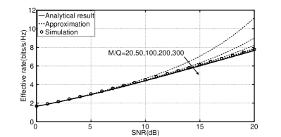
Figure 2: Effective rate using different discretization and truncation ratio $\frac{M}{Q}$ compared with analytical results and simulation results in i.i.d. generalized $K$ fading scenario.

The i.i.d. conditions are special cases in i.n.i.d. conditions. In order to verify the proposed approximation methods with existing results, the analytical results are estimated using [8, eq.(53)] and the parameters used in [8] are exploited. When approximating the effective rate using (31) in Theorem 4, the truncation parameter $Q$ can be chosen by a small number in practice, which is due to the fact that the estimated integration involving exponential fading terms. From the simulation experiments, we find that $Q=15$ is good enough for the estimation purpose, where further increase of the value of $Q$ will not give more accurate results. By increasing the ratio of the discretization parameter $M$ and the truncation parameter $Q$, the approximation approaches the exact value, as shown in Fig. 2. It is shown that when $M/Q\geq 200$, the approximations are tight with the simulation as well as analytical results, which supports the validation of the proposed approximation method. In the following part, $M/Q$ is selected as 300 as default, which gives good accuracy as well as low computational complexity.

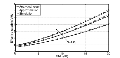
Figure 3: Effective rate over SISO and i.n.i.d. MISO fading channels, where parameters for each channel are listed in Table II.

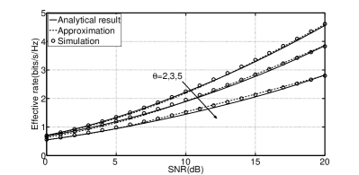
Figure 4: Effective rate under different QoS exponential $\theta$ in i.n.i.d. Weibull/Gamma fading channels with $N=2$.

In order to test the performance of the proposed methods under i.n.i.d. MISO fading channel conditions, different fading parameters and channel numbers are used, which are detailed in Table II. For different scenarios, it is shown in Fig. 3 that the approximations are sufficiently tight across a wide range of SNR (in this case from 0 to 20 dB) under different scenarios. Since the effective rate over i.n.i.d. MISO fading channels can be estimated based on the product of the individual channel’s MGF as presented in Thereom 4, the proposed MGF based approach is flexible and easy to extend.

Effective rate under different QoS exponent $\theta$ is the most interested parameter in the applications, since it can be used as a metric in the QoS provisioning schemes. Larger QoS exponent $\theta$ corresponds to tighter delay constraint. As shown in Fig. 4, the maximum available data rate drops with the increase of QoS exponent $\theta$, in order to guarantee the system’s delay performance. Also when the SNR gets higher, the same increase of $\theta$ results in greater drop of the effective rate.

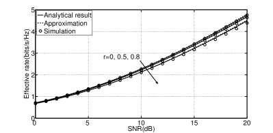
Figure 5: Effective rate under correlated generalized $K$ fading channel with different correlation coefficients $r=0,0.5,0.8$ and $N=2$, where approximation results are compared to analytical results and simulation results.

Furthermore, the effective rate over correlated generalized $K$ fading channels is investigated, whose channel fading parameters are given in Table II. It is shown in Fig. 5 that the effective rate reduces as the correlation coefficient $r$ increases from 0 to 0.8, where the case of $r=0$ corresponds to i.i.d. generalized $K$ fading channels.

VII Conclusion

In this paper, a new MGF based approach for the effective rate analysis over arbitrary correlated and not necessarily identical MISO fading channels using H transform representation has been proposed. The proposed framework has simplified the representation and analyses of effective rate in a unified way. The effective rate over i.n.i.d. hyper Fox’s H fading channels as well as arbitrary correlated generalized $K$ fading channels has been investigated, which has given good demonstrations on the application of the proposed MGF based approaches. Based on these results, the effective rate over many practical fading channels can be obtained by simply substituting the corresponding parameters instead of the cumbersome case-by-case integration procedure.

In addition, approximations have been given for the MGF based effective rate representation as well as the effective rate representation over i.n.i.d. MISO hyper Fox’s H fading channels, where both the truncation error and discretization error have been studied. These results have been illustrated readily applicable to practical fading channels, such as Weibull/Gamma and generalized $K$ fading channels. The simulations have been used to show the validation and accuracy of the proposed analytical and approximation methods. These results have extended and complemented the existing research of effective rate analysis.

We highlight that, as various metrics in wireless communication networks can be represented in similar H transform format and multivariate Fox’s H functions have the possibility to characterize the statistical properties of both independent and correlated channels, the obtained results will be also valuable to the performance analyses of other statistical metrics in wireless systems.

-A Fox’s H function, multivariate Fox’s H function and H transform

The Fox’s H function [23, Ch. 1.2] $H^{m{,}n}_{p{,}q}\left[\cdot\right]$, or univariate Fox’s H function in order to distinguish from multivariate Fox’s H function, can be defined by a single Mellin-Barnes type of contour integral as [23, Ch. 1.2]

$$H\left[s,\mathbf{O},\mathbf{P}\right]{=}uH^{m{,}n}_{p{,}q}\left[vs{\bigg{|}}\begin{matrix}\mathbf{c},\mathbf{C}\\ \mathbf{d},\mathbf{D}\end{matrix}\right]{=}\frac{u}{2\pi i}\oint_{\mathcal{L}}\Phi\left(z\right)(vs)^{z}dz,$$ (33)

where $i=\sqrt{-1}$, $s\neq 0$ and $\mathcal{L}$ is a suitable contour. The following notation is used for simplicity,

$$\left\{\begin{aligned} \mathbf{O}&=\left(m,n,p,q\right)\\ \mathbf{P}&=\left(u,v,\mathbf{c},\mathbf{d},\mathbf{C},\mathbf{D}\right)\end{aligned}\right.$$ (34)

where $\mathbf{c}{=}(\dot{\mathbf{c}}{,}\ddot{\mathbf{c}})$, $\mathbf{d}{=}(\dot{\mathbf{d}},\ddot{\mathbf{d}})$, $\mathbf{C}{=}(\dot{\mathbf{C}}{,}\ddot{\mathbf{C}})$ and $\mathbf{D}{=}(\dot{\mathbf{D}}{,}\ddot{\mathbf{D}})$, with $\dot{\mathbf{c}}{=}(c_{1}{,}\dots,c_{n})$, $\ddot{\mathbf{c}}{=}(c_{n+1}{,}\dots,c_{p})$, $\dot{\mathbf{d}}{=}(d_{1}{,}\dots,d_{m})$, $\ddot{\mathbf{d}}{=}(d_{m+1}{,}\dots,d_{q})$, $\dot{\mathbf{C}}{=}(C_{1}{,}\dots,C_{n})$, $\ddot{\mathbf{C}}{=}(C_{n+1}{,}\dots,C_{p})$, $\dot{\mathbf{D}}{=}(D_{1}{,}\dots,D_{m})$ and $\ddot{\mathbf{D}}{=}(D_{m+1}{,}\dots,D_{q})$. Also

$$\Phi\left(z\right){=}\frac{\prod_{j{=}1}^{m}\Gamma\left(d_{j}{-}D_{j}z\right)\prod_{j{=}1}^{n}\Gamma\left(1{-}c_{j}{+}C_{j}z\right)}{\prod_{j{=}n{+}1}^{p}\Gamma\left(c_{j}{-}C_{j}z\right)\prod_{j{=}m{+}1}^{q}\Gamma\left(1{-}d_{j}{+}D_{j}z\right)}.$$ (35)

Typical operations used in H transform are defined as follows[20]. The convolution operation is defined by $\mathbf{O}_{1}\boxplus\mathbf{O}_{2}=(m_{1}+m_{2},n_{1}+n_{2},p_{1}+p_{2},q_{1}+q_{2})$ and $\mathbf{P}_{1}\boxplus\mathbf{P}_{2}=(u_{1}u_{2},v_{1}v_{2},\mathbf{c}^{\prime},\mathbf{d}^{\prime},\mathbf{C}^{\prime},\mathbf{D}^{\prime})$, where $\mathbf{c}^{\prime}=(\dot{\mathbf{c}}_{1},\mathbf{c}_{2},\ddot{\mathbf{c}}_{1})$, $\mathbf{d}^{\prime}=(\dot{\mathbf{d}}_{1},\mathbf{d}_{2},\ddot{\mathbf{d}}_{1})$, $\mathbf{C}^{\prime}=(\dot{\mathbf{C}}_{1},\mathbf{C}_{2},\ddot{\mathbf{C}}_{1})$ and $\mathbf{D}^{\prime}=(\dot{\mathbf{D}}_{1},\mathbf{D}_{2},\ddot{\mathbf{D}}_{1})$. The Mellin operation is defined by $\mathbf{O}_{1}\boxdot\mathbf{O}_{2}=(m_{1}+n_{2},m_{2}+n_{1},p_{1}+q_{2},p_{2}+q_{1})$ and $\mathbf{P}_{1}\boxdot\mathbf{P}_{2}=(\frac{u_{1}u_{2}}{v_{2}},\frac{v_{1}}{v_{2}},\mathbf{c}^{\prime\prime},\mathbf{d}^{\prime\prime},\mathbf{C}^{\prime\prime},\mathbf{D}^{\prime\prime})$, where $\mathbf{c}^{\prime\prime}=(\dot{\mathbf{c}}_{1},\mathbf{1}_{q_{2}}-\mathbf{d}_{2}-\mathbf{D}_{2},\ddot{\mathbf{c}}_{1})$, $\mathbf{d}^{\prime\prime}=(\dot{\mathbf{d}}_{1},\mathbf{1}_{p_{2}}-\mathbf{c}_{2}-\mathbf{C}_{2},\ddot{\mathbf{d}}_{1})$, $\mathbf{C}^{\prime\prime}=(\dot{\mathbf{C}}_{1},\mathbf{D}_{2},\ddot{\mathbf{C}}_{1})$ and $\mathbf{D}^{\prime\prime}=(\dot{\mathbf{D}}_{1},\mathbf{C}_{2},\ddot{\mathbf{D}}_{1})$. Moreover, the scaling operation $\mathbf{P}|\alpha\rangle$ is defined by $\left(u/\alpha,v/\alpha,\mathbf{c},\mathbf{d},\mathbf{C},\mathbf{D}\right)$, while the elementary operation $\langle\alpha,\beta,\gamma|\mathbf{P}$ is defined by $\left(u/{(\alpha v)}^{\beta\gamma},{(\alpha v)}^{\beta},\mathbf{c}+\beta\gamma\mathbf{C},\mathbf{d}+\beta\gamma\mathbf{D},\beta\mathbf{C},\beta\mathbf{D}\right)$. Interested reader should refer to [20] for full details.

The operator $H^{0{,}n_{0}{;}m_{1}{,}n_{1}{;}\dots;m_{N}{,}n_{N}}_{p_{0}{,}q_{0}{;}p_{1}{,}q_{1}{;}\dots;p_{N}{,}q_{N}}\left[\cdot\right]$ is Fox’s H function of $N$ variables[23, Appendix A.1], or multivariate Fox’s H function for simplicity, which can be defined in terms of multiple Mellin-Barnes type contour integrals as

$$H^{0{,}n_{0}}_{p_{0}{,}q_{0}}\!\left[\begin{matrix}(a_{j}{;}A_{j}^{\left(1\right)}{,}{\dots}{,}A_{j}^{\left(N\right)})_{1{,}p_{0}}\\ (b_{j}{;}B_{j}^{\left(1\right)}{,}{\dots}{,}B_{j}^{\left(N\right)})_{1{,}q_{0}}\end{matrix}{:}\left(s_{j}{,}\mathbf{O}_{j}{,}\mathbf{P}_{j}\right)_{1{,}N}\right]$$ (36)

$${=} \frac{u_{1}{\cdots}u_{N}}{(2\pi i)^{N}}\int_{\mathcal{L}_{1}}\!\!\!{\cdots}\!\!\!\int_{\mathcal{L}_{N}}\!\Psi(\bm{\zeta})\left\{\prod^{N}_{j=1}\Phi_{j}(\zeta_{j})(v_{j}s_{j})^{\zeta_{j}}\right\}d\zeta_{1}{\cdots}d\zeta_{N},$$

where

$$\Psi(\bm{\zeta}){=}\frac{\prod\limits_{j{=}1}^{n_{0}}\!\Gamma(1{-}a_{j}{+}\sum\limits_{\ell{=}1}^{N}\!A_{j}^{(\ell)}\zeta_{\ell})}{\prod\limits_{j{=}n_{0}{+}1}^{p_{0}}\!\Gamma(a_{j}{-}\!\sum\limits_{\ell{=}1}^{N}A_{j}^{(\ell)}\!\zeta_{\ell})\prod\limits_{j{=}1}^{q_{0}}\!\Gamma(1{-}b_{j}{+}\!\sum\limits_{\ell{=}1}^{N}B_{j}^{(\ell)}\zeta_{\ell})},$$ (37)

$$\Phi_{j}(\zeta_{j}){=}\frac{\prod\limits_{\ell{=}1}^{m_{j}}\Gamma(d_{\ell}^{(j)}{-}D_{\ell}^{(j)}\zeta_{j})\prod\limits_{\ell{=}1}^{n_{j}}\Gamma(1{-}c_{\ell}^{(j)}{+}C_{\ell}^{(j)}\zeta_{j})}{\prod\limits_{\ell{=}n_{j}{+}1}^{p_{j}}\Gamma(c_{\ell}^{(j)}{-}C_{\ell}^{(j)}\zeta_{j})\prod\limits_{\ell{=}m_{j}{+}1}^{q_{j}}\Gamma(1{-}d_{\ell}^{(j)}{+}D_{\ell}^{(j)}\zeta_{j})},$$ (38)

whereas $\mathcal{L}_{j}$ is the suitable contours in the $\zeta_{j}$-plane. $(a_{j};A_{j}^{(1)},\dots,A_{j}^{\left(N\right)})_{1,p_{0}}$ abbreviates $p_{0}$-parameter array $(a_{1};A_{1}^{\left(1\right)},\dots,A_{1}^{\left(N\right)}),\dots,(a_{p_{0}};A_{p_{0}}^{\left(1\right)},\dots,A_{p_{0}}^{\left(N\right)})$, and $\left(s_{j},\mathbf{O}_{j},\mathbf{P}_{j}\right)_{1,N}$ abbreviates $N$-parameter array $\left\{s_{1},\mathbf{O}_{1},\mathbf{P}_{1};\cdots;s_{N},\mathbf{O}_{N},\mathbf{P}_{N}\right\}$, where $\mathbf{O}_{j}=(m_{j},n_{j},p_{j},q_{j})$ and
$\mathbf{P}_{j}=(u_{j},v_{j},\mathbf{c}^{(j)},\mathbf{d}^{(j)},\mathbf{C}^{(j)},\mathbf{D}^{(j)})$, whereas $\mathbf{c}^{(j)}$ abbreviates $p_{j}$-parameter array $(c_{1}^{(j)},\dots,c_{p_{j}}^{(j)})$. Other abbreviations follow the same way. See [23] for more related details.

Specially, when $n_{0}=p_{0}=q_{0}=0$, the multivariate Fox’s H function breaks up into the product of $N$ univariate Fox’s H functions as [23, eq.(A.13)]

$$H^{0{,}0}_{0{,}0}\left[\begin{matrix}{\textbf{---}}\\ {\textbf{---}}\end{matrix}{:}\left(s_{j}{,}\mathbf{O}_{j}{,}\mathbf{P}_{j}\right)_{1{,}N}\right]{=}\prod_{j{=}1}^{N}H\left[s_{j}{,}\mathbf{O}_{j}{,}\mathbf{P}_{j}\right].$$ (39)

The H transform of a function $f(z)$ with Fox’s H kernel is defined by [20]

$$\mathbb{H}\left\{f(z),\mathbf{O},\mathbf{P}\right\}(s){=}u\int_{0}^{\infty}\!H_{p{,}q}^{m{,}n}\left[vsz{\bigg{|}}\begin{matrix}\mathbf{c},\mathbf{C}\\ \mathbf{d},\mathbf{D}\end{matrix}\right]f(z)dz,$$ (40)

given that the integral converges absolutely and $s>0$.

-B Proof of Theorem 1

Using [20, eq.(28)] with the identity of [23, eq.(1.39)], [23, eq.(1.43)] and [23, eq.(2.22)] we have

$$H^{1{,}1}_{1{,}1}\left[\frac{\rho\sum_{j=1}^{N}\gamma_{j}}{N}{\bigg{|}}\begin{matrix}1{-}A{,}1\\ 0{,}1\end{matrix}\right]$$ (41)

$${=} \int_{0}^{\infty}\!\!H^{1{,}0}_{0{,}1}\left[s{\bigg{|}}\begin{matrix}{\textbf{---}}\\ A{-}1{,}1\end{matrix}\right]H^{1{,}0}_{0{,}1}\left[\frac{\rho s\sum_{j=1}^{N}\gamma_{j}}{N}{\bigg{|}}\begin{matrix}{\textbf{---}}\\ 0{,}1\end{matrix}\right]ds.$$

Substituting [23, eq.(1.43)] into (5) and using (41) as well as [20, eq.(62)], the following equation can be obtained

$$R(\theta) {=}{-}\frac{1}{A}\log_{2}\frac{1}{\Gamma(A)}\int_{0}^{\infty}H^{1{,}0}_{0{,}1}\left[s{\bigg{|}}\begin{matrix}{\textbf{---}}\\ A{-}1{,}1\end{matrix}\right]\phi_{\text{end}}\left(\frac{\rho s}{N}\right)ds.$$ (42)

Then use the definition of H transform (40), (6) can be achieved. By changing the integral variate, an alternative form can be obtained as (7).

-C Proof of Lemma 2

Using the H transform definition (40), the integration form can be obtained. First we prove that the integration can be truncated. Use the fact $\frac{\partial\phi(s)}{\partial s}<0$ for $s\in[0,\infty)$, the truncation error $E(Q)$ can be upper bounded by

$$E(Q) =\int_{Q}^{\infty}e^{{-}s}s^{A{-}1}\phi_{{\text{end}}}(\frac{s}{N})ds\leq\Gamma(A,Q),$$ (43)

where $\Gamma(A,Q)$ is the incomplete gamma function [41, eq.(8.350.2)]. Since the integrands in (43) are all positive for $s\in[0,\infty)$, then $E(Q)\geq 0$. Apply the Trapezoidal rules [21, eq.(3.5.2)] to evaluate the finite integration, then (26) and (28) can be obtained. Follow the limitation rules, we get (29).

References

- [1] D. Wu and R. Negi, “Effective capacity: A wireless link model for support of quality of service,” IEEE Trans. Wireless Commun., vol. 2, no. 4, pp. 630–643, Jul. 2003.
- [2] A. Khalek and Z. Dawy, “Energy-efficient cooperative video distribution with statistical QoS provisions over wireless networks,” IEEE Trans. Mobile Comput., vol. 11, no. 7, pp. 1223–1236, Jul. 2012.
- [3] A. Balasubramanian and S. Miller, “The effective capacity of a time division downlink scheduling system,” IEEE Trans. Commun., vol. 58, no. 1, pp. 73–78, Jan. 2010.
- [4] S. Agarwal, S. De, S. Kumar, and H. Gupta, “QoS-aware downlink cooperation for cell-edge and handoff users,” IEEE Trans. Veh. Technol., vol. 64, no. 6, pp. 2512–2527, Jun. 2015.
- [5] D. Qiao, M. Gursoy, and S. Velipasalar, “Effective capacity of two-hop wireless communication systems,” IEEE Trans. Inf. Theory, vol. 59, no. 2, pp. 873–885, Feb. 2013.
- [6] S. Akin and M. C. Gursoy, “Effective capacity analysis of cognitive radio channels for quality of service provisioning,” IEEE Trans. Commun., vol. 9, no. 11, pp. 3354–3364, Nov. 2010.
- [7] Y. Yang, S. Aissa, and K. Salama, “Spectrum band selection in delay-QoS constrained cognitive radio networks,” IEEE Trans. Veh. Technol., vol. 64, no. 7, pp. 2925–2937, Jul. 2015.
- [8] M. Matthaiou, G. C. Alexandropoulos, H. Q. Ngo, and E. G. Larsson, “Analytic framework for the effective rate of MISO fading channels,” IEEE Trans. Commun., vol. 60, no. 6, pp. 1741–1751, Jun. 2012.
- [9] M. You, H. Sun, J. Jiang, and J. Zhang, “Effective rate analysis in Weibull fading channels,” IEEE Wireless Commun. Lett., vol. 5, no. 4, pp. 340–343, Apr. 2016.
- [10] J. Zhang, M. Matthaiou, Z. Tan, and H. Wang, “Effective rate analysis of MISO - fading channels,” in Proc. IEEE Int. Conf. Commun. (ICC), Budapest, Jun. 2013, pp. 5840–5844.
- [11] J. Zhang, L. Dai, Z. Wang, D. Ng, and W. Gerstacker, “Effective rate analysis of MISO systems over - fading channels,” in Proc. Global Communications Conference (GLOBECOM), San Diego, CA, Dec. 2015, pp. 1–6.
- [12] J. Zhang, L. Dai, W. H. Gerstacker, and Z. Wang, “Effective capacity of communication systems over shadowed fading channels,” Electron. Lett., vol. 51, no. 19, pp. 1540–1942, Sep. 2015.
- [13] C. Zhong, T. Ratnarajah, K. K. Wong, and M. S. Alouini, “Effective capacity of correlated MISO channels,” in Proc. IEEE Int. Conf. Commun. (ICC), Kyoto, Jun. 2011, pp. 1–5.
- [14] X. B. Guo, L. Dong, and H. Yang, “Performance analysis for effective rate of correlated MISO fading channels,” Electron. Lett., vol. 48, no. 24, pp. 1564–1565, November 2012.
- [15] F. Yilmaz and M. Alouini, “A unified MGF-based capacity analysis of diversity combiners over generalized fading channels,” IEEE Trans. Commun., vol. 60, no. 3, pp. 862–875, Mar. 2012.
- [16] M. Di Renzo, F. Graziosi, and F. Santucci, “Channel capacity over generalized fading channels: A novel MGF-based approach for performance analysis and design of wireless communication systems,” IEEE Trans. Veh. Technol., vol. 59, no. 1, pp. 127–149, Jan. 2010.
- [17] Y. C. K. Ko, M. S. Alouini, and M. K. Simon, “Outage probability of diversity systems over generalized fading channels,” IEEE Trans. Commun., vol. 48, no. 11, pp. 1783–1787, Nov. 2000.
- [18] Z. Ji, C. Dong, Y. Wang, and J. Lu, “On the analysis of effective capacity over generalized fading channels,” in Proc. IEEE Int. Conf. Commu. (ICC), Sydney, Jun. 2014, pp. 1977–1983.
- [19] K. Peppas, P. T. Mathiopoulos, and J. Yang, “On the effective capacity of amplify-and-forward multi-hop transmission over arbitrary and correlated fading channels,” IEEE Wireless Commun. Lett., vol. PP, no. 99, pp. 1–1, 2016.
- [20] Y. Jeong, H. Shin, and M. Win, “H-transforms for wireless communication,” IEEE Trans. Inf. Theory, vol. 61, no. 7, pp. 3773–3809, Jul. 2015.
- [21] F. W. Olver, D. W. Lozier, R. F. Boisvert, and C. W. Clark, NIST handbook of mathematical functions. Washington, DC: Cambridge University Press, 2010.
- [22] M. C. Gursoy, “MIMO wireless communications under statistical queueing constraints,” IEEE Trans. Inf. Theory, vol. 57, no. 9, pp. 5897–5917, Sep. 2011.
- [23] A. M. Mathai, R. K. Saxena, and H. J. Haubold, The H-function: theory and applications, 2010th ed. Springer Science & Business Media, Oct. 2009.
- [24] F. Yilmaz and M. S. Alouini, “A novel unified expression for the capacity and bit error probability of wireless communication systems over generalized fading channels,” IEEE Trans. Commun., vol. 60, no. 7, pp. 1862–1876, Jul. 2012.
- [25] J. Zhang, Z. Tan, H. Wang, Q. Huang, and L. Hanzo, “The effective throughput of MISO systems over fading channels,” IEEE Trans. Veh. Technol., vol. 63, no. 2, pp. 943–947, Feb. 2014.
- [26] J. I. D. Cook, “The H-function and probability density functions of certain algebraic combinations of independent random variables with H-function probability distribution,” Ph.D. dissertation, Univ. Texas, Austin, TX, USA, 1981.
- [27] B. D. Carter, “On the probability distribution of rational functions of independent H-function variates,” Ph.D. dissertation, Univ. Arkansas, Fayetteville, AR, USA, 1972.
- [28] H. Srivastava and M. Garg, “Some integrals involving a general class of polynomials and the multivariable H-function,” Rev. Roumaine Phys., vol. 22, pp. 685–692, 1987.
- [29] R. Saxena, “On the H-function of n variables,” Kyungpook Math J, vol. 17, pp. 221–226, 1977.
- [30] S. Gaboury and R. Tremblay, “An expansion theorem involving H-function of several complex variables,” Int. J. Analysis, 2013.
- [31] H. Srivastava and R. Panda, “Expansion theorems for the H function of several complex variables,” J. Reine Angew. Math, vol. 288, pp. 129–145, 1976.
- [32] H. Srivastava and N. Singh, “The integration of certain products of the multivariable H-function with a general class of polynomials,” Rendiconti del Circolo Matematico di Palermo, vol. 32, no. 2, pp. 157–187, 1983.
- [33] B. D. Carter and M. D. Springer, “The distribution of products, quotients and powers of independent H-function variates,” SIAM J. Appl. Math., vol. 33, no. 4, pp. 542–558, Aug. 1977.
- [34] IEEE Vehicular Technology Society Committee on Radio Propagation, “Coverage prediction for mobile radio systems operating in the 800/900 MHz frequency range,” IEEE Trans. Veh. Technol., vol. 37, no. 1, pp. 3–72, Feb. 1988.
- [35] H. Srivastava, “A class of generalised multiple hypergeometric series arising in physical and quantum chemical applications,” J. Physics A: Mathematical and General, vol. 18, no. 5, p. 227, 1985.
- [36] R. Barakat, “Weak-scatterer generalization of the K-density function with application to laser scattering in atmospheric turbulence,” J. OSA. A., vol. 3, no. 4, pp. 401–409, Apr. 1986.
- [37] J. Zhang, M. Matthaiou, G. K. Karagiannidis, and L. Dai, “On the multivariate gamma-gamma distribution with arbitrary correlation and applications in wireless communications,” IEEE Trans. Veh. Technol., vol. 65, no. 5, pp. 3834–3840, May 2016.
- [38] P. Bithas, “Weibull-gamma composite distribution: alternative multipath/shadowing fading model,” Electron. Lett., vol. 45, no. 14, pp. 749–751, Jul. 2009.
- [39] F. Yilmaz and M. S. Alouini, “Product of the powers of generalized Nakagami- variates and performance of cascaded fading channels,” in Proc. IEEE Global Commun. Conf. (GLOBECOM), Honolulu, Nov. 2009, pp. 1–8.
- [40] H. R. Alhennawi, M. M. H. E. Ayadi, M. H. Ismail, and H. A. M. Mourad, “Closed-form exact and asymptotic expressions for the symbol error rate and capacity of the H -function fading channel,” IEEE Trans. Veh. Technol., vol. 65, no. 4, pp. 1957–1974, Apr. 2016.
- [41] I. S. Gradshteyn and I. M. Ryzhik, Table of integrals, series, and products, 6th ed. Academic Press, 2000.