LPSC16xxx

December 2016

Towards a new paradigm for quark-lepton unification

Christopher Smith^∗
Laboratoire de Physique Subatomique et de Cosmologie, Université Grenoble-Alpes, CNRS/IN2P3, 53 avenue des Martyrs, 38026 Grenoble Cedex, France.

Abstract

The quark and lepton mass patterns upset their naïve unification. In this paper, a new approach to solve this problem is proposed. Model-independently, we find that a successful unification can be achieved. A mechanism is identified by which the large top quark mass renders its third-generation leptonic partner very light. This state is thus identified with the electron. We then provide a generic dynamical implementation of this mechanism, using tree-level exchanges of vector leptons to relate the quark and lepton flavor structures. In a supersymmetric context, this same mechanism splits the squark masses, and third generation squarks end up much lighter than the others. Finally, the implementation of this mechanism in SU(5) GUT permits to avoid introducing any flavor structure beyond the two minimal Yukawa couplings, ensuring the absence of unknown mixing matrices and their potentially large impact on FCNC.

1 Introduction

Unifying all the fundamental constituents of matter has long been a major goal of particle physics. Yet, before the advent of the Standard Model (SM), the hadronic and leptonic particles have lived in opposite corners of our theories. With strikingly distinct dynamics and properties, it seemed the intimate nature of these particles were very different. This is well illustrated by the elusive neutrinos, and the contentious conservation of lepton number. At the same time, the much heavier protons and neutrons were still thought to be elementary, and baryon number was, naturally, thought to be conserved.

This state of matter was of course mostly due to the strong interaction. Once its veil is lifted, the quarks no longer seem so different from the leptons. Their share similar weak and electromagnetic interactions, as well as the mysterious family replication. In this sense, the SM represents the first true milestone in their unification. As a kind of puzzling bonus, the SM also hints at a higher level of unification. Indeed, its renormalizability, hence its whole internal coherence, rests on the consistency between the strong and electromagnetic charges of its fermionic constituents. In addition, baryon and lepton numbers are not conserved in the SM, but instead the non-perturbative electroweak interactions can for example transmute three leptons into nine antiquarks [1].

Soon after the SM was formulated as a spontaneously broken gauge theory, the same receipt was used to construct Grand Unified Theories based on larger gauge groups [2, 3]. There, not only the interactions but also all the matter content get embedded together in some representations of the unified gauge group. Quarks and leptons become manifestations of the same fundamental states, and GUT gauge interactions can transform one into the other. These inspiring theories, however, suffer many defects yet to be explained, most notably the stability of their scalar sector and their prediction that the proton should decay at rates now excluded.

Whether GUT represents a true second milestone towards quark-lepton unification is not so clear though. Indeed, embedding them in common representations only reproduces the coherence of their strong and electromagnetic charge we already had to impose to ensure the SM renormalizability. This may be seen as an explanation, or as a kind of unavoidable coincidence. Worse still, minimal GUT predicts simple relations between quark and lepton masses, in gross disagreement with the observed values. The only known way out of this conundrum is to somewhat relax their unification. Disappointingly, additional Yukawa interactions have to be introduced for the sole purpose of lifting the very prediction of unification.

The goal of this paper is to analyze the question of quark-lepton unification. For that, in the next Section, we first take a step back from GUT and characterize in a model independent setting the misalignment between the quark and lepton Yukawa couplings. Our strategy is to start by assuming

$$\mathbf{Y}_{e}=f(\mathbf{Y}_{d},\mathbf{Y}_{u})\;,$$ (1)

for some polynomial function $f$. Then, some requirements for a successful unification can be deduced from the peculiarities of this function $f$, which is found to be severely fine-tuned. In the following section, quite generic dynamical models are constructed to alleviate this fine-tuning, and thereby to automatically and naturally relate the quark and lepton flavor structures. The implications of such models for supersymmetry are discussed in Section 4, and its implementation within the minimal SU(5) model is described in Section  5. For simplicity, neutrinos are considered massless throughout this paper. The perspectives for neutrino mass models, as well as for other theories, are summarized in the conclusion.

2 Flavor symmetric perspective on quark-lepton unification

The strategy of choice when discussing the flavor sector of any theory is to identify the flavor symmetry and its explicit breaking terms. This permits to systematically work out and characterize their impacts on observables. In Section 2.1, we thus start by a brief summary of this technique, along with the closely related Minimal Flavor Violation (MFV) hypothesis. This sets the stage for Section 2.2, where this hypothesis is reinterpreted and adapted to the problem at hand, which is to relate the quark and lepton Yukawa couplings. Then, in Section 2.3, the peculiar fine-tuning of any relationship between $\mathbf{Y}_{e}$, $\mathbf{Y}_{d}$, and $\mathbf{Y}_{u}$ is identified, and some generic implications for the lepton mass spectrum are obtained. This information will guide us in the design of specific models in Section 3.

2.1 SM flavors and Minimal Flavor Violation

In the SM, the three generations of matter fields can be freely and independently redefined for each matter species without affecting the gauge sector, which thus has the symmetry [4]

$$G_{F}\equiv U(3)^{5}=U\left(3\right)_{Q}\otimes U\left(3\right)_{U}\otimes U\left(3\right)_{D}\otimes U\left(3\right)_{L}\otimes U\left(3\right)_{E}\;,$$ (2)

where $Q=(u_{L},d_{L})$, $U=u_{R}$, $D=d_{R}$, $L=(\nu_{L},e_{L})$, and $E=e_{R}$. This symmetry is broken by the Yukawa couplings only, which generate fermion masses and mixing after the electroweak symmetry breaking (EWSB). For the following, it will prove useful to immediately generalize to a Two Higgs Doublet Model (THDM) of type II, i.e.,

$$\mathcal{L}_{Y}=\bar{U}\mathbf{Y}_{u}QH_{u}+\bar{D}\mathbf{Y}_{d}QH_{d}+\bar{E}\mathbf{Y}_{e}LH_{d}\;,$$ (3)

because then the respective normalization of the up and down quark Yukawa couplings are tuned by the ratio of vacuum expectation values (VEV) $v_{u,d}$ of the two neutral Higgs components $H_{u,d}^{0}$, conventionally denoted as $\tan\beta=v_{u}/v_{d}$.

As is customary, to systematically investigate the impact of these symmetry breaking terms on observables, we first promote them to spurions. The idea is to artificially restore the $G_{F}$ symmetry by assigning definite $G_{F}$ transformation properties to the Yukawa couplings,

$$\mathbf{Y}_{u}\rightarrow g_{U}\mathbf{Y}_{u}g_{Q}^{\dagger},\;\;\mathbf{Y}_{d}\rightarrow g_{D}\mathbf{Y}_{d}g_{Q}^{\dagger},\;\;\mathbf{Y}_{e}\rightarrow g_{E}\mathbf{Y}_{e}g_{L}^{\dagger}\;,$$ (4)

where $g_{X}\in U(3)_{X}$, so that Eq. (3) becomes invariant under $X\rightarrow g_{X}X$. At this stage, the SM Lagrangian becomes invariant under $G_{F}$. Even if this is purely artificial, the amplitude for any possible process must also be expressible as manifestly $G_{F}$-invariant, and crucially, this may require inserting Yukawa spurions in a very specific way in the amplitude. The $G_{F}$ symmetry thus offers a very simple tool to predict the flavor structure of observables.

In a second stage, the spurion are frozen back to their physical values to get quantitative predictions. The Yukawa couplings admit the Singular Value Decompositions (SVD)

$$v_{u}\mathbf{Y}_{u}=\bar{g}_{U}^{\dagger}\mathbf{m}_{u}\bar{g}_{Q}^{u},\;\;v_{d}\mathbf{Y}_{d}=\bar{g}_{D}^{\dagger}\mathbf{m}_{d}\bar{g}_{Q}^{d}\;,\;\;v_{d}\mathbf{Y}_{e}=\bar{g}_{E}^{\dagger}\mathbf{m}_{d}\bar{g}_{L}\;,$$ (5)

for some (fixed) $\bar{g}_{X}$ transformations. So, using the $G_{F}$ invariance, it is always possible to freeze the Yukawa couplings at the values

$$v_{u}\mathbf{Y}_{u}=\mathbf{m}_{u}V,\;\;v_{d}\mathbf{Y}_{d}=\mathbf{m}_{d},\;\;v_{d}\mathbf{Y}_{e}=\mathbf{m}_{e}\;,$$ (6)

with $\mathbf{m}_{u,d,e}=\operatorname{diag}(m_{u,d,e},m_{c,s,\mu},m_{t,b,\tau})$ the diagonal mass matrices and $V=\bar{g}_{Q}^{u\dagger}\bar{g}_{Q}^{d}$ the CKM matrix. In this basis, the down quarks are all mass eigenstates, but not the left-handed up quarks. Whenever convenient, the $v_{u}\mathbf{Y}_{u}=\mathbf{m}_{u}$ and $v_{d}\mathbf{Y}_{d}=\mathbf{m}_{d}V^{\dagger}$ background values can also be chosen; the final results will obviously not depend on this choice.

In the presence of New Physics (NP), assuming gauge interactions still exhibit the $G_{F}$ symmetry, the same strategy as in the SM can be followed. In general, there will be additional flavored couplings, which have thus to be also promoted to spurions to restore the global $G_{F}$ symmetry. But because these new flavor couplings are a priori generic, they could induce unacceptably large effects in flavor observables when the New Physics scale is around the TeV [5]. On the contrary, this flavor puzzle disappears if the hierarchies of the NP flavor couplings are similar to those observed for the quark and lepton masses and mixings.

This is where the Minimal Flavor Violation hypothesis comes into play [6]. It is a tool designed to systematically export the numerical hierarchies of $\mathbf{Y}_{u,d,e}$ to the NP flavor sector, and proceeds in two steps [7]:

• Minimality: the first step is to remove the NP couplings from the spurion list. Only $\mathbf{Y}_{u,d,e}$ are kept in order to induce the known fermion mass. This does not forbid the NP couplings, but forces them to be expressed as polynomial expansions in $\mathbf{Y}_{u,d,e}$, as dictated by the $G_{F}$ symmetry.

• Naturality: The second step requires all the free parameters to be natural, i.e., the coefficients appearing in the spurion expansions have to be $\mathcal{O}(1)$. This ensures that the numerical hierarchies of $\mathbf{Y}_{u,d,e}$ are indeed passed on the NP couplings.

Provided these two conditions are met, the flavor observables are only marginally affected by TeV NP, and the flavor puzzles are solved. We refer to Ref. [5] for more information.

2.2 Fundamental flavor structures: Going beyond MFV

Naively, MFV seems to treat very differently the Yukawa couplings and the NP flavor couplings since the latter are expressed in terms of the former. For the following, it is crucial to understand that this asymmetrical treatment of a priori analogous Lagrangian couplings is more a matter of convenience than a statement about their respective nature. Indeed, MFV can be interpreted as a simple assumption about the mechanism at the origin of all the flavor structures [8].

To illustrate this, imagine a low-energy theory with two elementary flavor couplings $\mathbf{Y}$ and $\mathbf{A}$, which can be thought of as the Yukawa and NP couplings. At the very high scale, some flavor dynamics is active and introduces a single explicit breaking of $G_{F}$, which we call $\mathbf{X}$. The two low-energy flavor couplings are induced by this elementary flavor breaking, so it must be possible to relate them. For example, if $\mathbf{Y}$, $\mathbf{A}$, and $\mathbf{X}$ all transform under the same adjoint representation of some flavor $SU(3)\subset G_{F}$,

$$\left\{\begin{array}[c]{l}\mathbf{Y}=x_{1}^{Y}\mathbf{1}+x_{2}^{Y}\mathbf{X}+x_{3}^{Y}\mathbf{X}^{2}\;,\;\vskip 3.0pt plus 1.0pt minus 1.0pt\\ \mathbf{A}=x_{1}^{A}\mathbf{1}+x_{2}^{A}\mathbf{X}+x_{3}^{A}\mathbf{X}^{2}\;.\end{array}\right.$$ (7)

If the flavor dynamics was known, these coefficients could be computed explicitly. Lacking this, we simply assume they are natural. Also, for these expansions to make sense, powers of $\mathbf{X}$ must not grow unchecked. A sufficient condition is for the trace $\langle\mathbf{X}\rangle\lesssim 1$, since then all $\mathbf{X}^{n>2}$ can be eliminated in terms of $\mathbf{1}$, $\mathbf{X}$, and $\mathbf{X}^{2}$ without upsetting $x_{i}\sim\mathcal{O}(1)$ by using Cayley-Hamilton identities. Under this condition, from Eq. (7), we can get rid of the unknown high-energy spurion $\mathbf{X}$ and derive the low-energy MFV expansions

$$\left\{\begin{array}[c]{l}\mathbf{A}=y_{1}\mathbf{1}+y_{2}\mathbf{Y}+y_{3}\mathbf{Y}^{2}\;,\;\vskip 3.0pt plus 1.0pt minus 1.0pt\\ \mathbf{Y}=a_{1}\mathbf{1}+a_{2}\mathbf{A}+a_{3}\mathbf{A}^{2}\;,\end{array}\right.$$ (8)

for some $y_{i},a_{i}$ coefficients. Naturality is preserved since $y_{i},a_{i}\sim\mathcal{O}(1)$ when $x_{i}\sim\mathcal{O}(1)$ and $\langle\mathbf{X}\rangle\lesssim\mathcal{O}(1)$. In practice, only the first identity expressing $\mathbf{A}$ in terms of $\mathbf{Y}$ is useful since $\mathbf{Y}$ is known but $\mathbf{A}$ is not. So, in this interpretation, neither the Yukawa $\mathbf{Y}$ nor the NP coupling $\mathbf{A}$ are fundamental, and the MFV expansions are understood as the only low-energy observable consequences of their intrinsic redundancy.

In this paper, the basic hypothesis we wish to test is the redundancy of the SM Yukawa couplings themselves. MFV usually assumes the minimal spurion content to be $\mathbf{Y}_{u,d,e}$, so that all fermion masses can be induced. Here, we want to go beyond that and express some Yukawa couplings as expansions in others, as would happen if there are less than three fundamental flavor couplings.

To achieve this, as a first step, we have to restrict $G_{F}$ to a smaller group $G_{F}^{\prime}$, identify the reduced set of spurions, and fix their transformation properties under $G_{F}^{\prime}$. There is a priori a great latitude in these various choices and we do not plan to study them exhaustively. Instead, with GUT settings in mind, we consider only the continuous subgroups obtained by forcing some of the $U(3)$ transformations to be related. In other words, from a generic transformation $(g_{U},g_{D},g_{Q},g_{E},g_{L})\in G_{F}$, those of $G_{F}^{\prime}$ are obtained by imposing the equality (modulo transpositions and/or conjugations) of some of the $g_{i}$’s.

To further restrict the possibilities, we require

1. Naturality. With their two indices, the Yukawa couplings could transform as $\mathbf{1}$, $\mathbf{3}$, $\mathbf{6}$, or $\mathbf{8}$ under a given flavor $SU(3)$ or as $(\mathbf{3},\mathbf{3})$ under two different $SU(3)$s. But, given the very hierarchical form of the Yukawa couplings, naturality forbids any MFV expansion from starting as $\mathbf{Y}_{i}=a_{1}\mathbf{1}+...$, ruling out scenarios where $\mathbf{Y}_{i}\sim\mathbf{1}\oplus\mathbf{8}$ for some $i$. Also, if there is only one Higgs doublets, or if $\tan\beta$ is not very large when there are two doublets, then $G_{F}^{\prime}$ must forbid $\mathbf{Y}_{u}$ from contributing directly to $\mathbf{Y}_{d}$ or $\mathbf{Y}_{e}$. For example, if $G_{F}^{\prime}$ allows $\mathbf{Y}_{e}=a_{1}\mathbf{Y}_{u}+...$ , then $a_{1}$ would have to be very small.

2. Predictivity. When the group $G_{F}^{\prime}$ is too large compared to the number of spurions, they can all be diagonalized and no flavor mixing would survive. Conversely, if $G_{F}^{\prime}$ is too small compared to the number of spurions, unknown mixing matrices render the MFV expansions unpredictive. So $G_{F}^{\prime}$ has to give just enough freedom to rotate all the chosen spurions to their physical background values (as is the case in the usual MFV, see Eq. (6)). It is then possible to bring these spurions to their background values wherever they appear within the MFV expansions since these are $G_{F}^{\prime}$ invariant by construction.

In view of these points, there remain not so many viable scenarios. We need to keep at least two spurions, the symmetry group $G_{F}^{\prime}$ has to be large enough to account for the CKM mixing, and $\mathbf{Y}_{e,d}$ must transform differently than $\mathbf{Y}_{u}$. The simplest choice is to associate $\mathbf{Y}_{d}$ and $\mathbf{Y}_{e}$. For instance, if we take

$$G_{F}^{\prime}=U(3)^{3}=U\left(3\right)_{Q=L}\otimes U\left(3\right)_{U}\otimes U\left(3\right)_{D=E}\;,$$

then $\mathbf{Y}_{d}$ and $\mathbf{Y}_{e}$ transforms identically. Since only the misalignment between $\mathbf{Y}_{u}$ and $\mathbf{Y}_{d}$ is known, and not that between quark and lepton Yukawa couplings, the two spurions are chosen to be

$$\mathbf{Y}_{u}\rightarrow g_{U}\mathbf{Y}_{u}g_{Q}^{\dagger},\;\;\mathbf{Y}_{d}\rightarrow g_{D}\mathbf{Y}_{d}g_{Q}^{\dagger}\;,$$ (9)

whose background values can be fixed as in Eq. (6). This pattern is chosen also to allow for a smooth extension to GUT settings [9], as will be discussed later on.

2.3 Lepton masses from quark Yukawas

The next step is to express $\mathbf{Y}_{e}$ as a $G_{F}^{\prime}$-symmetric expansion in $\mathbf{Y}_{u}$ and $\mathbf{Y}_{d}$. From a mathematical point of view, any coupling can be expressed in this way, since together with their powers they form a complete basis for complex three-by-three matrices [10, 11]. What matters is the size of the expansion coefficients. Generic matrices expanded in such a basis require huge coefficients, while we are after $\mathcal{O}(1)$ ones for naturality reasons.

To illustrate this, consider the most general expansion, given the $G_{F}^{\prime}$ properties,

$$\mathbf{Y}_{e} =c_{0}\mathbf{Y}_{d}\cdot(\mathbf{1}+c_{1}\mathbf{Y}_{u}^{\dagger}\mathbf{Y}_{u}+c_{2}\mathbf{Y}_{d}^{\dagger}\mathbf{Y}_{d}+c_{3}(\mathbf{Y}_{u}^{\dagger}\mathbf{Y}_{u})^{2}+c_{4}(\mathbf{Y}_{d}^{\dagger}\mathbf{Y}_{d})^{2}+c_{5}\{\mathbf{Y}_{u}^{\dagger}\mathbf{Y}_{u},\mathbf{Y}_{d}^{\dagger}\mathbf{Y}_{d}\}$$

$$\;\;\;\;\;\;\;\;\;\;\;\;\;\;\;\;+ic_{6}[\mathbf{Y}_{u}^{\dagger}\mathbf{Y}_{u},\mathbf{Y}_{d}^{\dagger}\mathbf{Y}_{d}]+ic_{7}[(\mathbf{Y}_{u}^{\dagger}\mathbf{Y}_{u})^{2},\mathbf{Y}_{d}^{\dagger}\mathbf{Y}_{d}]+ic_{8}[\mathbf{Y}_{u}^{\dagger}\mathbf{Y}_{u},(\mathbf{Y}_{d}^{\dagger}\mathbf{Y}_{d})^{2}])\;.$$ (10)

If we require that this equation holds exactly once $\mathbf{Y}_{u,d,e}$ are replaced by their background values Eq. (6), then only terms involving $\mathbf{Y}_{d}$ can contribute since $\mathbf{Y}_{u}$ is not diagonal. The equation can nevertheless be solved but huge coefficients are required

$$c_{0}=0.2\;,\;\;c_{2}=7\times 10^{7}\times r_{\beta}^{2}\;,\;\;c_{4}=-3\times 10^{11}\times r_{\beta}^{4}\;,\;\;c_{i\neq 2,4}=0\;,$$ (11)

where $r_{\beta}=50/\tan\beta$ encodes a simplified $\tan\beta$ scaling, valid for $\tan\beta\gtrsim 5$. This is way beyond natural, but sets the stage against which we can compare more realistic settings. Also, it serves to illustrate how sensitive the coefficients are when trying to fit even slight misalignments.

Of course, it makes no sense to require $\mathbf{Y}_{e}$ to be diagonal in the basis in which $v_{u}\mathbf{Y}_{u}=\mathbf{m}_{u}V$ and $v_{d}\mathbf{Y}_{d}=\mathbf{m}_{d}$. Once the consequence of $G_{F}^{\prime}$ are worked out, the leptons are free to be rotated independently of the quarks. So, all that is required is for the three singular values of $v_{d}\mathbf{Y}_{e}$ to match the observed lepton masses. This means that there are only three constraints to solve for the nine a priori complex coefficients, leaving a large under-determination. To cure for this, we start by keeping only the three simplest terms in the expansion and set

$$c_{i\geq 3}\equiv 0\;.$$ (12)

Restricting coefficients to real values, and using the fermion masses quoted in Ref. [12] for several scenarios, we find

Masses at$$\text{\thinspace}M_{Z}:\;\;$$

THDM

                 (13)

The sign of $c_{0}$ is not fixed since it is irrelevant for the SVD values. Allowing for all the terms of Eq. (10) permits to reduce $c_{1,2}$ a bit but does not change their order of magnitude.

It is truly remarkable that it is possible for at least some of the scenarios to obtain natural values for the expansion coefficients. The most natural values arise at the EW scale, when $\tan\beta$ is sufficiently large to make $\mathbf{Y}_{d}^{\dagger}\mathbf{Y}_{d}$ entries of comparable size to those of $\mathbf{Y}_{u}^{\dagger}\mathbf{Y}_{u}$. Beyond that scale, the RG evolution under the MSSM or THDM at moderate or high $\tan\beta$ is strongly favored, while that of the SM departs from naturality essentially because $\tan\beta=1$, and also because the specific hierarchies of the Yukawa couplings becomes less compatible.

2.3.1 On the anatomy of a fine-tuning

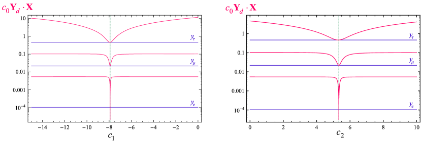
Figure 1: Evolution of the singular values of $\mathbf{Y}_{e}=c_{0}\mathbf{Y}_{d}\cdot\mathbf{X}$, with $\mathbf{X}\equiv\mathbf{1}+c_{1}\mathbf{Y}_{u}^{\dagger}\mathbf{Y}_{u}+c_{2}\mathbf{Y}_{d}^{\dagger}\mathbf{Y}_{d}$, as a function of the coefficient $c_{1}$ or $c_{2}$, holding the other parameters fixed. This evolution is very smooth, except for the dip occurring when $c_{1}$ or $c_{2}$ is such that $\det\mathbf{X}=0$. The green dashed lines indicate the point at which the singular values of $\mathbf{Y}_{e}$ coincide with the observed lepton Yukawa couplings, which clearly sits deep inside the dip (these values correspond to the MSSM at the GUT scale and $\tan\beta=50$, see Eq. (13)).

The size of the coefficients is not the only measure of naturalness. Despite their reasonable appearance, these expansions are severely fined-tuned. The behavior of the singular values when one of the expansion parameters is allowed to vary is shown in Fig. 1. Clearly, the polynomial expansion with natural coefficients has a marginal effect and the singular values stay very close to those of $c_{0}\times\mathbf{Y}_{d}$ except for a peculiar point where they all suddenly dip. If we denote the polynomial

$$\mathbf{X}\equiv\mathbf{1}+c_{1}\mathbf{Y}_{u}^{\dagger}\mathbf{Y}_{u}+c_{2}\mathbf{Y}_{d}^{\dagger}\mathbf{Y}_{d}\;,$$ (14)

so that $\mathbf{Y}_{e}=c_{0}\mathbf{Y}_{d}\cdot\mathbf{X}$, what happens at that point is a near cancellation

$$1\approx\mathbf{X}^{11}\approx\mathbf{X}^{22}\gg\mathbf{X}^{33}\approx 0\;.$$ (15)

For example, in the MSSM at $\tan\beta=50$,

$$|\mathbf{X}|=\left(\begin{array}[c]{ccc}1&0.0005&0.01\\ 0.0005&1&0.06\\ 0.01&0.06&0.004\end{array}\right)\;.$$ (16)

The eigenvalues of this polynomial show an even more striking hierarchy, with $v_{1}=1.0017$, $v_{2}=1.0000$, but $v_{3}=0.00026$. It is this peculiar feature which permits to significantly twist the singular values of $\mathbf{Y}_{d}$ to reproduce those of $\mathbf{Y}_{e}$.

To better understand why, in the basis Eq. (6), the $33$ entry seem to play a particular role, let us take the determinant of Eq. (10). The unknown SVD matrices are unitary and disappear, leaving

$$\det(\mathbf{Y}_{e})=c_{0}^{3}\times\det(\mathbf{Y}_{d})\times\det(\mathbf{1}+c_{1}\mathbf{Y}_{u}^{\dagger}\mathbf{Y}_{u}+c_{2}\mathbf{Y}_{d}^{\dagger}\mathbf{Y}_{d})\;.$$ (17)

The dip shown in Fig. 1 corresponds to the point where $\det\mathbf{X}$ vanishes. Using Cayley-Hamilton identities and thanks to the large hierarchy of the Yukawa couplings, $(\mathbf{Y}_{i}^{\dagger}\mathbf{Y}_{i})^{2}\approx\langle\mathbf{Y}_{i}^{\dagger}\mathbf{Y}_{i}\rangle\mathbf{Y}_{i}^{\dagger}\mathbf{Y}_{i}$, $i=u,d$,

$$\det(\mathbf{1}+c_{1}\mathbf{Y}_{u}^{\dagger}\mathbf{Y}_{u}+c_{2}\mathbf{Y}_{d}^{\dagger}\mathbf{Y}_{d})\approx 1+c_{1}\langle\mathbf{Y}_{u}^{\dagger}\mathbf{Y}_{u}\rangle+c_{2}\langle\mathbf{Y}_{d}^{\dagger}\mathbf{Y}_{d}\rangle\approx 0\;.$$ (18)

In the basis Eq. (6), this immediately implies Eq. (15) since the top and bottom Yukawa couplings dominate, $\langle\mathbf{Y}_{u,d}^{\dagger}\mathbf{Y}_{u,d}\rangle\approx y_{t,b}^{2}$ . The fact that natural coefficients are possible at all can thus be traced to the large $y_{t,b}^{2}$ couplings. In this sense, it looks truly remarkable that a solution where both $c_{1}$ and $c_{2}$ end up not larger than $\langle\mathbf{Y}_{u}^{\dagger}\mathbf{Y}_{u}\rangle^{-1}$ and $\langle\mathbf{Y}_{d}^{\dagger}\mathbf{Y}_{d}\rangle^{-1}$ exists. Still, at this stage, we cannot make the economy of a mechanism able to automatically ensure such a near cancellation of $\det(\mathbf{X})$.

As a side remark, it should be noted that solving Eq. (10) for $c_{0,1,2}$ given the singular values of $\mathbf{Y}_{e}$ is tricky. Indeed, singular value decompositions are highly non-linear, and the equations for $c_{0,1,2}$ cannot be solved exactly. Worse, once reverting to numerical methods, algorithms are very unstable because the solutions we are after lie in the very narrow valley where the required cancellation takes place.

2.3.2 The twisted persona of the leptons

Before turning to scenarios, there is another peculiar feature of the expansion worth discussing. The SVD of $\mathbf{Y}_{e}$ is $g_{E}\mathbf{Y}_{e}g_{L}^{\dagger}$, so let us look at the mixing matrices $g_{E}$ and $g_{L}^{\dagger}$ as one approaches the dip of Fig. 1. We thus take the MSSM at $\tan\beta=50$ and vary $c_{2}$ holding the other coefficients $c_{0,1}$ fixed. Away from the dip, the two unitary matrices deviate only slightly from identity

$$c_{2}=2.5:|g_{E}|=\left(\begin{array}[c]{ccc}1.000&0.00016&0.000054\\ 0.00016&1.000&0.0048\\ 0.000055&0.0048&1.000\end{array}\right)\;,\;\;|g_{L}|=\left(\begin{array}[c]{ccc}1.00&0.0050&0.038\\ 0.0019&0.98&0.18\\ 0.038&0.18&0.98\end{array}\right)\;.$$ (19)

Moving closer, the situation changes dramatically for $g_{L}$

$$c_{2}=4.8:|g_{E}|=\left(\begin{array}[c]{ccc}1.000&0.0084&0.0012\\ 0.0082&0.99&0.11\\ 0.0020&0.11&0.99\end{array}\right)\;,\;\;|g_{L}|=\left(\begin{array}[c]{ccc}0.98&0.13&0.14\\ 0.011&0.71&0.70\\ 0.20&0.69&0.70\end{array}\right)\;.$$ (20)

The reason for this large mixing in the left-handed lepton sector is the difference between

$$\mathbf{Y}_{e}^{\dagger}\mathbf{Y}_{e}=c_{0}^{2}\times\mathbf{X}\cdot\mathbf{Y}_{d}^{\dagger}\mathbf{Y}_{d}\cdot\mathbf{X}\;\text{ and}\;\;\;\mathbf{Y}_{e}\mathbf{Y}_{e}^{\dagger}=c_{0}^{2}\times\mathbf{Y}_{d}\cdot\mathbf{X}^{2}\cdot\mathbf{Y}_{d}^{\dagger}\;,$$ (21)

diagonalized by the unitary matrix $g_{L}$ and $g_{E}$, respectively. Because of Eq. (15), the entry $(\mathbf{Y}_{e}^{\dagger}\mathbf{Y}_{e})^{33}$ decreases approaching the dip, but this does not occur for $\mathbf{Y}_{e}\mathbf{Y}_{e}^{\dagger}$ whose diagonal entries always stay very hierarchical. The point $c_{2}=4.8$ corresponds to $(\mathbf{Y}_{e}^{\dagger}\mathbf{Y}_{e})^{33}\approx(\mathbf{Y}_{e}^{\dagger}\mathbf{Y}_{e})^{22}$, hence the large mixing present in $g_{L}$.

Moving even closer to the dip, $(\mathbf{Y}_{e}^{\dagger}\mathbf{Y}_{e})^{33}$ becomes smaller than $(\mathbf{Y}_{e}^{\dagger}\mathbf{Y}_{e})^{22}$ and the left-handed leptons get even more twisted:

$$c_{2}=5.2:|g_{E}|=\left(\begin{array}[c]{ccc}0.97&0.086&0.0023\\ 0.083&0.98&0.20\\ 0.020&0.20&0.98\end{array}\right)\;,\;\;|g_{L}|=\left(\begin{array}[c]{ccc}0.80&0.56&0.20\\ 0.033&0.28&0.96\\ 0.59&0.77&0.21\end{array}\right)\;.$$ (22)

At the $c_{2}$ value for which $g_{E}\mathbf{Y}_{e}g_{L}^{\dagger}=\mathbf{m}_{e}/v_{d}$, the mixings settle at

$$c_{2}=5.3:|g_{E}|=\left(\begin{array}[c]{ccc}0.97&0.24&0.0023\\ 0.24&0.95&0.22\\ 0.055&0.21&0.98\end{array}\right)\;,\;\;|g_{L}|=\left(\begin{array}[c]{ccc}0.032&0.98&0.20\\ 0.062&0.20&0.98\\ 1.00&0.019&0.068\end{array}\right)\;.$$ (23)

At this value, large mixing angles disappear and all mixings are CKM-like. Still, the left-handed leptons are irremediably twisted since

$$\left(\begin{array}[c]{c}e_{L}\\ \mu_{L}\\ \tau_{L}\end{array}\right)^{phys}\approx\left(\begin{array}[c]{ccc}0&0&1\\ 1&0&0\\ 0&1&0\end{array}\right)\cdot\left(\begin{array}[c]{c}e_{L}\\ \mu_{L}\\ \tau_{L}\end{array}\right)^{gauge}\;.$$ (24)

Note that this reordering of the leptonic states does not depend on the basis chosen for the quark Yukawa couplings in Eq. (6), contrary to the mixing angles in $g_{E}$ and $g_{L}$. In practice, as long as neutrinos are massless and in the absence of lepton-number violating couplings, neither these mixings nor the twist are observable. On the other hand, when studying the neutrino sector, especially mass hierarchies, such a twist could have great implications since the lightest left handed lepton would be essentially the third-generation gauge state.

As a final remark, it should be noted that the results of this section do not change if one identifies the flavor group as $U\left(3\right)_{Q=E}\otimes U\left(3\right)_{U}\otimes U\left(3\right)_{D=L}$ instead of $U\left(3\right)_{Q=L}\otimes U\left(3\right)_{U}\otimes U\left(3\right)_{D=E}$, except for the interchange of $g_{L}$ and $g_{E}$. Indeed, the SVD constraints imposing $\mathbf{Y}_{e}=c_{0}\mathbf{Y}_{d}\cdot\mathbf{X}$ or $\mathbf{Y}_{e}^{T}=c_{0}\mathbf{Y}_{d}\cdot\mathbf{X}$ are obviously identical, but for $g_{L}\leftrightarrow g_{E}$. The right-handed leptons would then be twisted, with no visible consequence on the neutrinos. Further, we will see in the next section that it is also possible to have double expansions like $\mathbf{Y}_{e}=c_{0}\mathbf{X\cdot Y}_{d}\cdot\mathbf{X}^{\prime}$ with both $\det\mathbf{X}$ and $\det\mathbf{X}^{\prime}$ close to zero, in which case right and left leptons end up simultaneously twisted. This should be kept in mind, especially as the $SU(5)$ unification pattern corresponds [9] to $U\left(3\right)_{Q=E=U}\otimes U\left(3\right)_{D=L}$, with $\mathbf{Y}_{u}\sim(\mathbf{\bar{6}},\mathbf{1})$ required to be symmetric, and $\mathbf{Y}_{d}\sim\mathbf{Y}_{e}^{T}\sim(\mathbf{\bar{3}},\mathbf{3})$.

3 Scenario 1: Light electrons from heavy tops

It is now time to devise a mechanism able to naturally tune the MFV expansion of $\mathbf{Y}_{e}$. In the next subsection, this problem is tackled from a mathematical point of view, and in the following, a corresponding physically plausible though quite generic scenario is presented.

3.1 The mathematics of infinite MFV expansions

Let us restate the problem at hand. We have seen that the expansion $\mathbf{Y}_{e}=c_{0}\mathbf{Y}_{d}\cdot\mathbf{X}$ requires $\mathbf{X}^{33}\approx 0$. This means, dropping $\mathbf{Y}_{d}^{\dagger}\mathbf{Y}_{d}$ for simplicity, that with

$$\mathbf{X}=\mathbf{1}+c\mathbf{Y}_{u}^{\dagger}\mathbf{Y}_{u}\;,$$ (25)

the coefficient must be tuned to

$$\det\mathbf{X}\approx 0\Rightarrow c\approx-\frac{1}{\langle\mathbf{Y}_{u}^{\dagger}\mathbf{Y}_{u}\rangle}\;.$$ (26)

Though the numerical value of $c$ is natural thanks to the large top quark Yukawa coupling, the fine-tuning between $c$ and $\langle\mathbf{Y}_{u}^{\dagger}\mathbf{Y}_{u}\rangle$ is unacceptable. Clearly, adding more terms to the $\mathbf{X}$ expansion cannot improve the situation. For example, if we add a term $c^{\prime}(\mathbf{Y}_{u}^{\dagger}\mathbf{Y}_{u})^{2}$ to $\mathbf{X}$, then both $c$ and $c^{\prime}$ have to be fined-tuned so that $\det\mathbf{X}\approx 0$. No finite polynomial in $\mathbf{Y}_{u}^{\dagger}\mathbf{Y}_{u}$ and/or $\mathbf{Y}_{d}^{\dagger}\mathbf{Y}_{d}$ would ever permit to relax the fine-tuning.

The key to solve this problem is to consider infinite polynomials. Consider for instance the geometric series

$$\mathbf{X}=\mathbf{1}+\eta\mathbf{Y}_{u}^{\dagger}\mathbf{Y}_{u}+\eta^{2}(\mathbf{Y}_{u}^{\dagger}\mathbf{Y}_{u})^{2}+\eta^{3}(\mathbf{Y}_{u}^{\dagger}\mathbf{Y}_{u})^{3}+...$$ (27)

Barring convergence issues to be discussed below, the sum is

$$\mathbf{X}=\frac{1}{\mathbf{1}-\eta\mathbf{Y}_{u}^{\dagger}\mathbf{Y}_{u}}\;.$$ (28)

This matrix has the desired property. In the diagonal basis, $\mathbf{Y}_{u}^{\dagger}\mathbf{Y}_{u}=\operatorname{diag}(y_{u}^{2},y_{c}^{2},y_{t}^{2})$ and

$$\mathbf{X}^{11,22}=\frac{1}{1-\eta y_{u,c}^{2}}\approx 1\;\;\text{but \ }\mathbf{X}^{33}=\frac{1}{1-\eta y_{t}^{2}}\approx 0\;,$$ (29)

whenever $\eta$ is large enough that $\eta y_{t}^{2}\gg 1$ but still small enough that $\eta y_{u,c}^{2}\ll 1$. Specifically, the large top quark mass translate into $(\mathbf{Y}_{u}^{\dagger}\mathbf{Y}_{u})^{2}\approx\langle\mathbf{Y}_{u}^{\dagger}\mathbf{Y}_{u}\rangle\mathbf{Y}_{u}^{\dagger}\mathbf{Y}_{u}$, so that

$$\mathbf{X=}\sum_{n=0}^{\infty}\eta^{n}(\mathbf{Y}_{u}^{\dagger}\mathbf{Y}_{u})^{n}\approx\mathbf{1}+\eta\mathbf{Y}_{u}^{\dagger}\mathbf{Y}_{u}\sum_{n=0}^{\infty}\eta^{n}\langle\mathbf{Y}_{u}^{\dagger}\mathbf{Y}_{u}\rangle^{n}=\mathbf{1}+\frac{\eta}{1-\eta\langle\mathbf{Y}_{u}^{\dagger}\mathbf{Y}_{u}\rangle}\mathbf{Y}_{u}^{\dagger}\mathbf{Y}_{u}\;,$$ (30)

which tends to

$$\mathbf{X}\overset{\eta\gg 1}{\approx}\mathbf{1}-\frac{1}{\langle\mathbf{Y}_{u}^{\dagger}\mathbf{Y}_{u}\rangle}\mathbf{Y}_{u}^{\dagger}\mathbf{Y}_{u}\;.$$ (31)

This is precisely the result we were after, Eqs. (25) and (26). Crucially, the value of $\eta$ does not need to have any precise relationship with $\langle\mathbf{Y}_{u}^{\dagger}\mathbf{Y}_{u}\rangle$, it just needs to be large enough so that $\eta\langle\mathbf{Y}_{u}^{\dagger}\mathbf{Y}_{u}\rangle\gg 1$.

Evidently, the suppression of $\mathbf{X}^{33}$ requires summing the geometric series well outside its radius of convergence. Even if one could argue that such series make sense through analytic continuation, as is customary for perturbative series in Quantum Field Theory, the situation is not very comfortable. One simple way out of possible convergence issues is to consider for example Eq. (28) as the true expression. In this way, even if the expanded form of the MFV polynomial does not converge from a strict mathematical sense, it should not have been trusted in the first place. We will see in the next section a practical realization of such a scenario. One should note also a peculiar feature of the geometric series involving matrices. Even if the infinite sum of powers does not converge, any inverse matrix can be expanded in a finite polynomial. Denoting $\mathbf{A}\equiv\eta\mathbf{Y}_{u}^{\dagger}\mathbf{Y}_{u}$ and using Cayley-Hamilton identities,

$$\frac{1}{\mathbf{1}+\mathbf{A}}=\frac{1}{\det(\mathbf{1}+\mathbf{A})}\left[\mathbf{1(}1+\langle\mathbf{A}\rangle+\frac{1}{2}(\langle\mathbf{A}\rangle^{2}-\langle\mathbf{A}^{2}\rangle))-\mathbf{A}\left(1+\langle\mathbf{A}\rangle\right)+\mathbf{A}^{2}\right]\;,$$ (32)

whenever

$$\det(\mathbf{1}+\mathbf{A})=1+\langle\mathbf{A}\rangle+\frac{1}{2}\langle\mathbf{A}\rangle^{2}-\frac{1}{2}(1+\langle\mathbf{A}\rangle)\langle\mathbf{A}^{2}\rangle+\frac{1}{3}\langle\mathbf{A}^{3}\rangle+\frac{1}{6}\langle\mathbf{A}\rangle^{3}\neq 0\;.$$ (33)

The result Eq. (31) is immediately obtained in the third generation dominance $\mathbf{A}^{2}\rightarrow\langle\mathbf{A}\rangle\mathbf{A}$, even though no resummation is implied.

All the discussions of this section can be extended to include both $\mathbf{A}\equiv\eta\mathbf{Y}_{u}^{\dagger}\mathbf{Y}_{u}$ and $\mathbf{B}\equiv\eta^{\prime}\mathbf{Y}_{d}^{\dagger}\mathbf{Y}_{d}$. The analytical expressions are more cumbersome since in general $[\mathbf{A},\mathbf{B}]\neq 0$. For example,

$$\mathbf{X}=(\mathbf{1}+\mathbf{A}+\mathbf{A}^{2}+...)(\mathbf{1}+\mathbf{B}+\mathbf{B}^{2}+...)=\frac{1}{\mathbf{1}+\mathbf{A}}\frac{1}{\mathbf{1}+\mathbf{B}}\approx\left(\mathbf{1}-\frac{\mathbf{A}}{1+\langle\mathbf{A}\rangle}\right)\left(\mathbf{1}-\frac{\mathbf{B}}{1+\langle\mathbf{B}\rangle}\right)\;,$$ (34)

where the last equality holds in the third-generation dominance approximation, or

$$\mathbf{X}=\mathbf{1}+\mathbf{A}+\mathbf{B}+(\mathbf{A}+\mathbf{B})^{2}+...=\frac{1}{\mathbf{1}+\mathbf{A}+\mathbf{B}}\approx\mathbf{1}-\frac{\mathbf{A}+\mathbf{B}}{1+\langle\mathbf{A}\rangle+\langle\mathbf{B}\rangle}\;.$$ (35)

Both these series manifestly reproduces the previous result $\mathbf{X}^{11},\mathbf{X}^{22}\gg\mathbf{X}^{33}\approx 0$ thanks to the large hierarchy in the $\mathbf{Y}_{u,d}$ couplings, and require analytical continuation to be defined outside of their radius of convergence.

3.2 Vector-like leptons and geometric Yukawas

To induce geometric-like MFV expansions, our strategy is to generate effective contributions to the Yukawa coupling $\mathbf{Y}_{e}$ through the tree-level exchange of new states. As such, it is a bit similar to the Froggatt-Nielsen mechanism [13], although the new fields will not introduce any new breaking of the flavor symmetry. Such breaking would not be adequate here since the goal is to generate the MFV series, not to explain the internal hierarchy of the Yukawa couplings themselves.

Specifically, consider adding to the SM a flavor-triplet of vector leptons $X_{L,R}$, having the same gauge quantum numbers as the lepton doublet, and a singlet scalar boson $H_{s}$. The new terms in the Lagrangian are, omitting flavor indices for simplicity

$$\mathcal{L}_{X_{L,R}} =\bar{X}_{L}(i\not{D})X_{L}+\bar{X}_{R}(i\not{D}))X_{R}+\bar{X}_{L}\mathbf{M}_{X}X_{R}+\bar{X}_{R}\mathbf{M}_{X}X_{L}\frac{{}}{{}}$$

$$+\left(\bar{X}_{R}\mathbf{N}_{X}X_{L}H_{s}+\bar{X}_{R}\mathbf{\bar{N}}_{X}LH_{s}+\bar{E}\mathbf{Y}_{X}X_{L}H_{d}+h.c.\frac{{}}{{}}\right)\;,$$ (36)

where $\mathbf{M}_{X}$, $\mathbf{N}_{X}$, $\mathbf{\bar{N}}_{X}$ and $\mathbf{Y}_{X}$ are all three-by-three matrices in flavor space. This model contains many new flavor couplings and flavored particles, so our starting point is to impose MFV. For that, we take the flavor symmetry

$$G_{F}^{\prime}=U\left(3\right)_{Q=L=X_{L,R}}\otimes U\left(3\right)_{U}\otimes U\left(3\right)_{D=E}\;,$$ (37)

with thus $X_{L,R}$ transforming like $L$ and $Q$, and allow only for $\mathbf{Y}_{u}$ and $\mathbf{Y}_{d}$ as spurions. The various flavor couplings can then all be expressed in terms of $\mathbf{Y}_{u}$ and $\mathbf{Y}_{d}$. We assume the simple expansions

$$\left\{\begin{array}[c]{c}\mathbf{M}_{X}=M_{X}\mathbf{1\;,}\\ \mathbf{Y}_{e}=\mathbf{Y}_{X}=\gamma\mathbf{Y}_{d}\;,\\ \mathbf{N}_{X}=\mathbf{\bar{N}}_{X}=\alpha\mathbf{Y}_{u}^{\dagger}\mathbf{Y}_{u}+\beta\mathbf{Y}_{d}^{\dagger}\mathbf{Y}_{d}\;,\end{array}\right.$$ (38)

where $\mathbf{Y}_{e}$ corresponds to the SM Yukawa interaction $E\mathbf{Y}_{e}LH_{d}$. A constant term in $\mathbf{N}_{X}=\mathbf{\bar{N}}_{X}$ is omitted even if it is consistent with $G_{F}^{\prime}$ for reasons that will be clear below, so we assume that these couplings disappear in the absence of $\mathbf{Y}_{u,d}$.

Figure 2: The effective contributions to the leptonic Yukawa couplings generated by the tree-level exchanges of (a) a flavor-triplet, weak doublet of vector leptons $X_{L,R}$ or (b) a flavor-triplet, weak singlet of vector leptons $Z_{L,R}$. When both these states are present, the two contributions (a) and (b) are accompanied by their simultaneous exchanges (c).

When the vector leptons are heavy, they can be integrated out by solving their equations of motion

$$\frac{\delta\mathcal{L}_{\xi}}{\delta X_{L}} =\bar{X}_{R}(\mathbf{M}_{X}+\mathbf{N}_{X}H_{s})+\bar{E}\mathbf{Y}_{X}H_{d}=0\;\;,$$ (39)

$$\frac{\delta\mathcal{L}_{\xi}}{\delta X_{R}} =\bar{X}_{L}(\mathbf{M}_{X}+\mathbf{N}_{X}^{\dagger}H_{s})+\bar{L}\mathbf{\bar{N}}_{X}^{\dagger}H_{s}=0\;.$$ (40)

Plugging this back into the Lagrangian, we get a contribution to the leptonic Yukawa interaction (see Fig. 2a)

$$\mathbf{Y}_{e}^{eff}=\mathbf{Y}_{e}-\mathbf{Y}_{X}\frac{1}{\mathbf{M}_{X}+\mathbf{N}_{X}H_{s}}\mathbf{\bar{N}}_{X}H_{s}=\gamma\mathbf{Y}_{d}\cdot\frac{\mathbf{1}}{\mathbf{1}+(v_{s}/M_{X})(\alpha\mathbf{Y}_{u}^{\dagger}\mathbf{Y}_{u}+\beta\mathbf{Y}_{d}^{\dagger}\mathbf{Y}_{d})}\;,$$ (41)

with $v_{s}$ the scalar singlet vacuum expectation value. Provided $v_{s}/M_{X}\gg 1$, this precisely reproduces the geometric sum discussed in the previous section. Importantly, no resummation was involved: the $X_{L,R}$ mass terms and their interactions with $H_{s}$ were integrated exactly. If these terms were treated perturbatively, one would recover a geometric MFV series. So, in this case, the issue of the convergence of the MFV series is really similar to that of the usual QFT perturbative series.

Numerically, we fix $\alpha$ and solve for the remaining parameters $\gamma$, $\beta$ and $v$ so that the three singular values $\mathbf{Y}_{e}^{eff}$ reproduce the observed lepton masses. For the MSSM at the GUT scale with $\tan\beta=10$, we find

$$\gamma=22\;,\;\;\alpha\equiv-1\;,\;\;\beta=-1.2\;,\;\;\frac{v_{s}}{M_{X}}=4\times 10^{4}\;.$$ (42)

The expansion coefficients are very reasonable when the ratio $v_{s}/M_{X}$ is large. Importantly, the value of $v_{s}$ is totally decorrelated from that of $\mathbf{Y}_{u}$ or $\mathbf{Y}_{d}$. As shown in Fig. 3, the evolution of the singular values of $\mathbf{Y}_{e}^{eff}$ as $v_{s}$ is varied is rather smooth over a large range (keep in mind though that the scale of the plot is logarithmic). The same is true when varying $\alpha$ or $\beta$, ensuring this solution is free of any fine-tuning.

The lepton mixing matrices at the best-fit point are

$$|g_{E}|=\left(\begin{array}[c]{ccc}0.96&0.26&0.0040\\ 0.24&0.88&0.42\\ 0.11&0.41&0.91\end{array}\right)\;,\;\;|g_{L}|=\left(\begin{array}[c]{ccc}0.0089&0.98&0.17\\ 0.038&0.17&0.98\\ 1.00&0.015&0.0036\end{array}\right)\;.$$ (43)

Compared to the mixing matrices obtained using the polynomial expansion, Eq. (23), the same twist of the left leptons happens while the mixing angles are a bit larger (smaller) in the right (left) sector.

Figure 3: Evolution of the singular values of $\mathbf{Y}_{e}^{eff}$ as given in Eq. 41, i.e., induced by tree-level exchanges of the vector leptons $X_{L,R}$. The green dashed line indicates the point at which the singular values of $\mathbf{Y}_{e}^{eff}$ coincide with the observed lepton Yukawa couplings, and corresponds to the values quoted in Eq. 42. Compared to Fig. 1, it now sits at a perfectly regular point. The singular values are not fine-tuned since they do not change much as the $\mathbf{Y}_{e}^{eff}$ parameters vary.

This setting can be generalized in many ways. One interesting extension is to introduce vector-like partners for both the lepton singlet and doublet. So, we add a flavor-triplet of vector leptons $Z_{L,R}$ transforming as the right-handed lepton singlet:

$$\mathcal{L}_{X_{L,R},Z_{L,R}} =\mathcal{L}_{X_{L,R}}+\bar{Z}_{L}(i\not{D})Z_{L}+\bar{Z}_{R}(i\not{D})Z_{R}+\bar{Z}_{L}\mathbf{M}_{Z}Z_{R}+\bar{Z}_{R}\mathbf{M}_{Z}Z_{L}\frac{{}}{{}}$$

$$+\left(\bar{Z}_{R}\mathbf{N}_{Z}Z_{L}H_{s}+\bar{E}\mathbf{\bar{N}}_{Z}Z_{L}H_{s}+\bar{Z}_{R}\mathbf{Y}_{Z}LH_{d}+h.c.\frac{{}}{{}}\right)$$

$$+\left(\bar{Z}_{R}\mathbf{Y}_{ZX}X_{L}H_{d}+\bar{X}_{R}\mathbf{Y}_{XZ}Z_{L}H_{d}+h.c.\frac{{}}{{}}\right)\;.$$ (44)

Choosing now the flavor symmetry as

$$G_{F}^{\prime}=U\left(3\right)_{Q=L=X_{L,R}}\otimes U\left(3\right)_{U}\otimes U\left(3\right)_{D=E=Z_{L,R}}\;,$$ (45)

the MFV assumptions become

$$\left\{\begin{array}[c]{c}\mathbf{M}_{X,Z}=M_{X,Z}\mathbf{1\;,}\\ \mathbf{Y}_{e}=\mathbf{Y}_{X}=\mathbf{Y}_{Z}=\mathbf{Y}_{XZ}=\mathbf{Y}_{ZX}=\gamma\mathbf{Y}_{d}\;,\\ \mathbf{N}_{X}=\mathbf{\bar{N}}_{X}=\alpha\mathbf{Y}_{u}^{\dagger}\mathbf{Y}_{u}+\beta\mathbf{Y}_{d}^{\dagger}\mathbf{Y}_{d}\;,\\ \mathbf{N}_{Z}=\mathbf{\bar{N}}_{Z}=\varepsilon\mathbf{Y}_{d}\mathbf{Y}_{d}^{\dagger}\;.\end{array}\right.$$ (46)

The equations of motion for the four families of heavy leptons $X_{L,R}$ and $Z_{L,R}$ are coupled because of the mixing term $\mathbf{Y}_{XZ}$ and $\mathbf{Y}_{ZX}$ but can be solved to first order in $H_{d}$ (see Fig. 2):

$$\mathbf{Y}_{e}^{eff} =\mathbf{Y}_{e}-\mathbf{Y}_{X}\frac{1}{\mathbf{M}_{X}+\mathbf{N}_{X}H_{s}}\mathbf{\bar{N}}_{X}H_{s}-H_{s}\mathbf{\bar{N}}_{Z}\frac{1}{\mathbf{M}_{Z}+\mathbf{N}_{Z}H_{s}}\mathbf{Y}_{Z}$$

$$\;\;\;\;\;\;\;\;\;\;\;\;\;\;\;\;\;\;\;\;+H_{s}\mathbf{\bar{N}}_{Z}\frac{1}{\mathbf{M}_{Z}+\mathbf{N}_{Z}H_{s}}\mathbf{Y}_{ZX}\frac{1}{\mathbf{M}_{X}+\mathbf{N}_{X}H_{s}}\mathbf{\bar{N}}_{X}H_{s}$$

$$=\frac{1}{\mathbf{1}+(v_{s}/M_{Z})(\varepsilon\mathbf{Y}_{d}\mathbf{Y}_{d}^{\dagger})}\cdot\gamma\mathbf{Y}_{d}\cdot\frac{1}{\mathbf{1}+(v_{s}/M_{X})(\alpha\mathbf{Y}_{u}^{\dagger}\mathbf{Y}_{u}+\beta\mathbf{Y}_{d}^{\dagger}\mathbf{Y}_{d})}\;.$$ (47)

By trial and error, we find for example for the MSSM at the GUT scale and $\tan\beta=30$,

$$\gamma=81\;,\;\alpha\equiv 1\;,\;\;\beta\equiv 1\;,\;\;\;\varepsilon\equiv-1\;,\;\;\;\frac{v_{s}}{M_{X}}=2.1\times 10^{3}\;,\;\;\frac{M_{X}}{M_{Z}}\equiv 7\;,$$ (48)

or

$$\gamma=83\;,\;\alpha\equiv 1\;,\;\;\beta\equiv 0\;,\;\;\;\varepsilon\equiv-1\;,\;\;\;\frac{v_{s}}{M_{X}}=1.1\times 10^{4}\;,\;\;\frac{M_{X}}{M_{Z}}\equiv 0.3\;.$$ (49)

Infinitely many other solutions exists, some may give slightly lower $v_{s}/M_{X,Z}$, but none should decrease it dramatically. Concentrating on the first solution, we show in Fig. 4 the behavior as $v_{s}$ varies holding the other parameters fixed. It is evidently free of any fine-tuning, and even more stable than before. Further, this solution has one very interesting feature. Once the right-handed sector becomes tuned by a geometric expansion, both species of leptons end up similarly twisted:

$$|g_{E}|=\left(\begin{array}[c]{ccc}0.015&1.00&0.0019\\ 0.0032&0.0018&1.00\\ 1.00&0.015&0.003\end{array}\right)\;,\;\;|g_{L}|=\left(\begin{array}[c]{ccc}0.0069&1.00&0.019\\ 0.032&0.020&1.00\\ 1.00&0.0075&0.031\end{array}\right)\;.$$ (50)

The mixing angles are also greatly reduced. This means that in this scenario, the true identity of the electron is completely altered: it is mostly the third-generation gauge state.

Figure 4: Evolution of the singular values of $\mathbf{Y}_{e}^{eff}$ as given in Eq. 3.2, i.e., induced by tree-level exchanges of both the vector leptons $X_{L,R}$ and $Z_{L,R}$. The green dashed line indicates the point at which the singular values of $\mathbf{Y}_{e}^{eff}$ coincide with the observed lepton Yukawa couplings, and corresponds to the values quoted in Eq. 48. Compared to Fig. 1, it now sits at a perfectly regular point, and compared to Fig. 3, even larger departures from that point have a negligible impact on the two largest singular values. The evolution as the other parameters are varied is similar as in Fig. 3.

These constructions are not meant to be full-fledged models. Rather, they are designed to illustrate the main mechanism by which the lepton and quark flavor structures could be related in a natural way. The most salient features are

• The value for $\gamma$ is often found a bit too large if one has in mind GUT settings where the boundary conditions set e.g. $\mathbf{Y}_{e}^{T}=\mathbf{Y}_{d}$. Still, the situation is different in GUT since both $\mathbf{Y}_{e}$ and $\mathbf{Y}_{d}$ have to be generated simultaneously out of other Yukawa couplings. This will be discussed in Section 5. Also, this value of $\gamma$ depends quite crucially on the value of $v_{s}$, and on the MFV conditions Eq. (38) or (46).

• The effective contribution to $\mathbf{Y}_{e}$ decouples when either $v_{s}\rightarrow 0$ or $M_{X,Z}\rightarrow\infty$, but is non-decoupling in the $v_{s}>M_{X,Z}$ region relevant for the geometric behavior.

• The scales $v_{s}$ and $M_{X,Z}$ are free since only their ratio plays a role. Further, any rescaling of the expansion coefficients in $\mathbf{N}_{X,Z}$ and $\mathbf{\bar{N}}_{X,Z}$ can be compensated by a change in $v_{s}/M_{X,Z}$. In particular, one could imagine that in some more complete model, $\mathbf{N}_{X,Z}$ and $\mathbf{\bar{N}}_{X,Z}$ are radiatively induced. This would naturally explain the specific form of their expansions in Eq. (38) or (46), at the cost of further increasing $v_{s}/M_{X,Z}$.

• Such large $v_{s}/M_{X,Z}$ ratios imply that $v_{s}\gg v_{u,d}$ since $M_{X,Z}$ should be above the EW scale for all the vector leptons to be integrated out. If not protected by some symmetry, this large hierarchy could require delicate fine-tunings in the scalar sector, in case $H_{s}$ couples to $H_{u}$ and/or $H_{d}$. Note though that in a supersymmetric setting, the only allowed superpotential term would be $H_{s}H_{u}H_{d}$, which breaks the Peccei-Quinn symmetry [14] if the couplings in Eq. (44) do not. Connection with invisible axion models [15], where large hierarchies are also present between symmetry breaking scales, could offer interesting perspective, which we leave for future works.

• The MFV conditions Eq. (38) or (46) could be thought of as boundary conditions, in a way similar to the mSUGRA pattern for supersymmetry breaking terms. But, looking at Eq. (41) or Eq. (46), it is clear that even small deviations from these conditions would spoil the geometric behavior for the MFV series.

Let us analyze this last point in a bit more detail. Indeed, it would not be very convincing to trade the fine-tunings in the coefficients in Eq. (13) for a fine-tuning in the boundary conditions. Ultimately, the mechanism at the origin of these conditions should be accompanied by a symmetry able to stabilize them, at least partially. Looking back at Eq. (44), we can already glean some hints of how this could arise. If we combine together the nine weak doublet lepton fields into $\Phi_{L}^{T}=(L,X_{L},X_{R})$ and the nine weak singlet lepton fields into $\Phi_{R}^{T}=(E,Z_{R},Z_{L})$, then

$$\mathcal{L}_{X_{L,R},Z_{L,R},E,L}=\bar{\Phi}_{L}(i\not{D}+\mathbf{P}_{X})\Phi_{L}+\bar{\Phi}_{R}(i\not{D}+\mathbf{P}_{Z})\Phi_{R}+(\bar{\Phi}_{R}\mathbf{Y}\Phi_{L}H_{d}+h.c.)\;,$$ (51)

actually exhibits a $U(9)_{L}\otimes U(9)_{R}$ flavor symmetry broken only by the flavor structures:

$$\mathbf{P}_{A}=\left(\begin{array}[c]{ccc}0&0&0\\ 0&0&\mathbf{M}_{A}\\ 0&\mathbf{M}_{A}&0\end{array}\right)+\left(\begin{array}[c]{ccc}0&0&\mathbf{\bar{N}}_{A}\\ 0&0&\mathbf{N}_{A}\\ \mathbf{\bar{N}}_{A}&\mathbf{N}_{A}&0\end{array}\right)H_{s},\;\;\mathbf{Y}=\left(\begin{array}[c]{ccc}\mathbf{Y}_{e}&\mathbf{Y}_{X}&0\\ \mathbf{Y}_{Z}&\mathbf{Y}_{ZX}&0\\ 0&0&\mathbf{Y}_{XZ}\end{array}\right)\;.$$ (52)

Most vanishing entries are due to chirality, the rest to the gauge symmetries. Consider then the $\mathbf{M}_{X,Z}=0$ limit. The MFV conditions Eq. (38) or (46) emerge as the only one invariant under $(X_{L}\leftrightarrow L)$ and $(Z_{R}\leftrightarrow E)$. Imagine thus that $H_{s}$ first gets its VEV at the scale $v_{s}$, while this discrete symmetry is broken spontaneously at the much lower scale $M_{X,Z}$. The deviations with respect to the conditions Eq. (38) or (46) would end up tiny, at most of the order of $M_{X,Z}/v_{s}$, and would not completely alter the $v_{s}$ scaling of $\mathbf{Y}_{e}^{eff}$. Actually, such corrections may even be welcome to reduce the numerical value of $\gamma$ or the ratio $v_{s}/M_{X,Z}$.

4 Scenario 2: Supersymmetry and light stops

Supersymmetry is one the most studied extension to the SM. Besides its intrinsic mathematical appeal, it is able to solve, or at least lessen, several puzzles of the SM, and most notably the issue of the stability of the electroweak scale. At the same time, low-scale supersymmetry is expected to influence various flavor physics observables, and its many new states are within range of direct production at the LHC. The absence of any signal up to now puts strong constraints on viable supersymmetric scenarios. Our goal in this section is to analyze in which respect the relationship discovered between $\mathbf{Y}_{e}$ and $\mathbf{Y}_{u,d}$ could help.

4.1 Squark mass matrices with geometric expansions

Direct searches for supersymmetric particles at colliders are particularly sensitive to first-generation squarks, simply because of the presence of many such quarks in the initial state. The current bounds are typically well above 1 TeV, depending on the assumptions on the masses of the other sparticles [16, 17]. On the contrary, for third generation squarks, the bounds are still below the TeV. In this context, Natural SUSY-like scenarios [18] where third generation squarks are much lighter than the others offer interesting settings. What we now want to show is that settings where all MFV expansions are geometric actually generate such patterns.

Consider the following geometric MFV parametrization for the squark soft-breaking terms

$$\mathbf{m}_{Q,U,D}^{2}=m_{0}^{2}\mathbf{X}_{Q,U,D}\;\;,\;\;\;\mathbf{A}_{u,d}=A_{0}\mathbf{X}_{U,D}\cdot\mathbf{Y}_{u,d}\cdot\mathbf{X}_{Q}\;,$$ (53)

with

$$\mathbf{X}_{Q} =\frac{1}{\mathbf{1}-\eta_{q}(\alpha_{1}^{q}\mathbf{Y}_{u}^{\dagger}\mathbf{Y}_{u}+\alpha_{2}^{q}\mathbf{Y}_{d}^{\dagger}\mathbf{Y}_{d}+...)}\;,$$ (54a)

$$\mathbf{X}_{U} =\frac{1}{\mathbf{1}-\eta_{u}(\alpha_{1}^{u}\mathbf{Y}_{u}\mathbf{Y}_{u}^{\dagger}+\alpha_{2}^{u}\mathbf{Y}_{u}\mathbf{Y}_{d}^{\dagger}\mathbf{Y}_{d}\mathbf{Y}_{u}^{\dagger}+...)}\;,$$ (54b)

$$\mathbf{X}_{D} =\frac{1}{\mathbf{1}-\eta_{d}(\alpha_{1}^{d}\mathbf{Y}_{d}\mathbf{Y}_{d}^{\dagger}+\alpha_{2}^{d}\mathbf{Y}_{d}\mathbf{Y}_{u}^{\dagger}\mathbf{Y}_{u}\mathbf{Y}_{d}^{\dagger}+...)}\;,$$ (54c)

where $$\alpha_{i}^{q,u,d} \mathcal{O}(1) m_{0} A_{0} m_{0}=10 A_{0}=-1 \mathbf{X}_{Q,U,D}$$ are parameters, , the SUSY-breaking scale parameters, which we set at TeV, TeV, and we assume are the same when entering squared squark masses or trilinear terms for simplicity

Though we will not attempt at constructing a fully dynamical model, it is tempting to think of these $\mathbf{X}_{Q}$, $\mathbf{X}_{U}$, and $\mathbf{X}_{D}$ factors as arising from the exchange of new states whose propagators transform like $SU(3)_{Q}$, $SU(3)_{U}$ or $SU(3)_{D}$ octets, respectively. The corresponding coefficients $\eta_{q,u,d}=v_{s}/M_{X_{Q,U,D}}$, with $M_{X_{Q,U,D}}$ the mass of these octets and $v_{s}$ the VEV of some singlet Higgs bosons, can in principle be large. These $\mathbf{X}_{Q,U,D}$ factor then match those studied in the previous section, with for example

$$\mathbf{X}_{U}\approx\mathbf{1}-\frac{1}{\langle\mathbf{Y}_{u}^{\dagger}\mathbf{Y}_{u}\rangle}\mathbf{Y}_{u}\mathbf{Y}_{u}^{\dagger}\;.$$ (55)

Note that it may make more sense to think of these new states as scalars, in which case $\mathbf{X}_{Q,U,D}^{2}$ propagator factors would appear in Eq. (53). Numerically, this would not change much the boundary conditions for the squark soft-breaking terms since the strict third-generation dominance approximation $(\mathbf{Y}_{i}^{\dagger}\mathbf{Y}_{i})^{2}\rightarrow\langle\mathbf{Y}_{i}^{\dagger}\mathbf{Y}_{i}\rangle\mathbf{Y}_{i}^{\dagger}\mathbf{Y}_{i}$ implies for example

$$\mathbf{X}_{U}^{2}\approx\left(\mathbf{1}-\frac{1}{\langle\mathbf{Y}_{u}^{\dagger}\mathbf{Y}_{u}\rangle}\mathbf{Y}_{u}\mathbf{Y}_{u}^{\dagger}\right)^{2}\approx\mathbf{1}-\frac{1}{\langle\mathbf{Y}_{u}^{\dagger}\mathbf{Y}_{u}\rangle}\mathbf{Y}_{u}\mathbf{Y}_{u}^{\dagger}\;.$$ (56)

For simplicity, we thus stick to the linear expansions in Eq. (53).

In the large $\eta_{q,u,d}$ limit, this setting actually matches that studied in Ref. [19] from a purely phenomenological perspective. There, the large $\eta_{q,u,d}$ limit of the expansions in Eq. (53) were imposed at the GUT scale and evolved down to the TeV scale. Let us summarize the main results:

• To end up with only the $\tilde{t}_{L}$ and $\tilde{b}_{L}$ as light states, one should set $\eta_{u,d}=0$, $\eta_{q}\gg 1$. However, the RG evolution necessarily drives the small $\mathbf{m}_{Q}^{2}[M_{GUT}]^{33}$ towards negative values. This results in an unacceptable color-breaking minimum. To prevent this, either one should impose Eq. (53) at a much lower scale, or $\mathbf{m}_{U}^{2}[M_{GUT}]^{33}$ must also be small. In this latter case, setting $\eta_{u}=\eta_{q}\gg 1$, the three squark states $\tilde{t}_{L,R}$ and $\tilde{b}_{L}$ end up much lighter than the other squarks, whose masses remain very close to $m_{0}$.

• Except at very large $\tan\beta$, the impact of $\mathbf{X}_{D}$ is always negligible and $\tilde{b}_{R}$ remains quasi-degenerate with the first- and second-generation squarks.

• The RG evolution of the trilinear terms $\mathbf{A}_{U,D}$ wipes out the effect of the $\mathbf{X}_{Q,U,D}$ factors. In other words, at the low scale, the trilinear terms obtained either from $\mathbf{A}_{U,D}[M_{GUT}]=A_{0}\mathbf{X}_{U,D}\cdot\mathbf{Y}_{u,d}\cdot\mathbf{X}_{Q}$ or simply from $\mathbf{A}_{U,D}[M_{GUT}]=A_{0}\mathbf{Y}_{u.d}$ are very similar, and so are the resulting squark mass spectra.

• Because $\langle\mathbf{Y}_{u}^{\dagger}\mathbf{Y}_{u}\rangle$ and $\langle\mathbf{Y}_{d}^{\dagger}\mathbf{Y}_{d}\rangle$ are at most $\mathcal{O}(1)$, these expansions satisfy the usual MFV naturality requirement. As a result, supersymmetric contributions to flavor transitions remain tuned by the CKM matrix, and the constraints from flavor observables are satisfied even with rather light sparticles.

4.2 Untwisted slepton mass matrices and $\mu\rightarrow e\gamma$

To express the lepton Yukawa coupling in terms of those of the quarks, the flavor symmetry was reduced to $G_{F}^{\prime}=U\left(3\right)_{Q=L}\otimes U\left(3\right)_{U}\otimes U\left(3\right)_{D=E}$. In a supersymmetric setting, $G_{F}^{\prime}$ also allows for the slepton soft-breaking terms to be expressed in terms of $\mathbf{Y}_{u,d}$. Altogether, the lepton and slepton flavor-breaking sector becomes

$$\mathbf{Y}_{e}=\gamma\mathbf{X}_{D}\cdot\mathbf{Y}_{d}\cdot\mathbf{X}_{Q}\;,$$ (57)

and

$$\mathbf{m}_{L}^{2}=m_{0}^{2}\mathbf{X}_{Q}\;,\;\;\mathbf{m}_{E}^{2}=m_{0}^{2}\mathbf{X}_{D}\;,\;\;\mathbf{A}_{e}=\gamma A_{0}\;\mathbf{X}_{D}\cdot\mathbf{Y}_{d}\cdot\mathbf{X}_{Q}\;.$$ (58)

For simplicity, we assume universal expansions in each $SU(3)$ sectors, i.e., all $\mathbf{X}_{Q}$ factors are identical, and so are all the $\mathbf{X}_{E}$.

Once these conditions are set, the freedom to rotate the (s)lepton doublet and singlet is recovered since the MSSM exhibit a $G_{F}$ symmetry in its gauge sector. Thus, $\mathbf{Y}_{e}$ can be diagonalized through

$$L\rightarrow g_{L}L,E\rightarrow g_{E}E,\;\;\mathbf{Y}_{e}\rightarrow(\mathbf{Y}_{e})^{phys}=g_{E}\mathbf{Y}_{e}g_{L}^{\dagger}\;,$$ (59)

with $(\mathbf{Y}_{e})^{phys}=\operatorname{diag}(y_{e},y_{\mu},y_{\tau})$. This same rotation has to be performed on the slepton partners, so that in the lepton physical basis,

$$(\mathbf{m}_{L}^{2})^{phys}=m_{0}^{2}g_{L}\mathbf{X}_{Q}g_{L}^{\dagger}\;,\;\;(\mathbf{m}_{E}^{2})^{phys}=m_{0}^{2}g_{E}\mathbf{X}_{D}g_{E}^{\dagger}\;,\;\;(\mathbf{A}_{e})^{phys}=A_{0}\mathbf{Y}_{e}\;.$$ (60)

This action of the mixing matrices $g_{L}$ and $g_{E}$ has two particularities. First, neither $(\mathbf{m}_{L}^{2})^{phys}$ nor $(\mathbf{m}_{E}^{2})^{phys}$ are diagonal in general, since the matrices $g_{E}$ and $g_{L}$ come from the SVD of $\mathbf{Y}_{e}$. Their off-diagonal entries are of the order of CKM entries, since they are generated by the mismatch between $\mathbf{Y}_{u}$ and $\mathbf{Y}_{d}$ entering in $\mathbf{X}_{Q,D}$. Second, even if $g_{L}$ and/or $g_{E}$ can twist the leptons, as in Eq. (43) or Eq. (50), this same twist is then enforced on their supersymmetric partners. For example, if only $\mathbf{X}_{Q}$ is present, $(e_{L}^{-})^{phys}$ is essentially the $(\tau_{L})^{gauge}$ state, then $(\tilde{e}_{L})^{phys}$ is essentially the $(\tilde{\tau}_{L})$ gauge state. Further, given that

$$1\approx(\mathbf{m}_{L}^{2})^{11}\approx(\mathbf{m}_{L}^{2})^{22}\gg(\mathbf{m}_{L}^{2})^{33}\approx 0\;,$$ (61)

the $(\tilde{e}_{L})^{phys}$ and $(\tilde{\nu}_{L})^{phys}$ states are much lighter than the other sleptons.

Non-vanishing off-diagonal entries in $(\mathbf{m}_{L}^{2})^{phys}$ together with rather light first-generation sleptons immediately raise the question of lepton flavor violating (LFV) observables. A process like $\mu\rightarrow e\gamma$ can be induced by neutralino and chargino loops, with a branching ratio scaling like [20]

$$\mathcal{B}(\mu\rightarrow e\gamma)\approx 10^{-5}\frac{M_{W}^{4}}{M_{\tilde{\ell}}^{8}}\tan\beta\left|(\mathbf{m}_{L}^{2})_{12}^{phys}\right|^{2}F_{SUSY}\;,$$ (62)

where $M_{\tilde{\ell}}$ is the typical slepton mass, which we take as the geometric average of the involved sleptons, $M_{\tilde{\ell}}^{2}=M_{\tilde{e}}M_{\tilde{\mu}}$, and $F_{SUSY}$ is an $\mathcal{O}(1)$ function of the sparticle masses. The question is then whether the current bound $\mathcal{B}(\mu\rightarrow e\gamma)^{\exp}<5.7\times 10^{-13}$ [21] is satisfied.

To illustrate that this is indeed the case, let us consider a specific realization. We set the boundary conditions at the GUT scale, and perform the evolution at NLO. For simplicity, we introduce only $\mathbf{X}_{Q}$ and not $\mathbf{X}_{D}$. The inputs at the GUT scale are slightly different than for Eq. (42), because of the specific MSSM parameters chosen here, and we take

$$\gamma=19\;,\;\;\alpha_{1}^{q}\equiv 1\;,\;\;\alpha_{2}^{q}=2.6\;,\;\;\eta_{q}=2.1\times 10^{4}\;.$$ (63)

Once $\mathbf{Y}_{e}=\gamma\mathbf{Y}_{d}\cdot\mathbf{X}_{Q}$ is fixed, $g_{L}$ and $\mathbf{m}_{L}^{2}=m_{0}^{2}\mathbf{X}_{Q}$ can be computed directly:

$$|g_{L}|=\left(\begin{array}[c]{ccc}0.0098&0.99&0.17\\ 0.041&0.17&0.98\\ 1.00&0.017&0.045\end{array}\right),\;\;|\mathbf{m}_{L}^{2}[M_{GUT}]|=m_{0}^{2}\left(\begin{array}[c]{ccc}0.99&0.045&0.0066\\ 0.045&0.74&0.029\\ 0.0066&0.029&0.0014\end{array}\right)\;,$$ (64)

so

$$|(\mathbf{m}_{L}^{2}[M_{GUT}])^{phys}|=m_{0}^{2}\left(\begin{array}[c]{ccc}0.00049&0.018&0.0015\\ 0.018&1.00&0.0029\\ 0.0015&0.0029&0.74\end{array}\right)\;.$$ (65)

Notice how acting with $g_{L}$ reorders the entries of $\mathbf{m}_{L}^{2}$. Evolving down, only the diagonal entries are significantly affected since $\mathbf{Y}_{e}$ is diagonal in the physical basis at all scale. For example, with $m_{0}=10$ TeV, we find at the low-scale,

$$|(\mathbf{m}_{L}^{2}[1\,\text{TeV}])^{phys}|=m_{0}^{2}\left(\begin{array}[c]{ccc}0.042&0.018&0.0015\\ 0.018&1.04&0.0029\\ 0.0015&0.0029&0.77\end{array}\right)\;.$$ (66)

This means that the current bound on $\mathcal{B}(\mu\rightarrow e\gamma)$ translate as a lower bound on $m_{0}$. Coincidentally, as plotted in Fig. 5, the current limit does not constrain $m_{0}$ much yet, but any improvement on $\mathcal{B}(\mu\rightarrow e\gamma)^{\exp}$ would start to push $m_{0}$ well beyond $1$ TeV. Note, finally, that setting $\mathbf{m}_{L}^{2}=m_{0}^{2}\mathbf{X}_{Q}^{2}$ instead of $\mathbf{m}_{L}^{2}=m_{0}^{2}\mathbf{X}_{Q}$ does not impact $\mathcal{B}(\mu\rightarrow e\gamma)$ significantly, since it would mean setting

$$|(\mathbf{m}_{L}^{2}[M_{GUT}])^{phys}|=m_{0}^{2}\left(\begin{array}[c]{ccc}0.00035&0.018&0.0052\\ 0.018&1.01&0.016\\ 0.0052&0.016&2.44\end{array}\right)\;.$$ (67)

Figure 5: Left slepton masses and $\mathcal{B}(\mu\rightarrow e\gamma)$ as a function of the SUSY breaking scale $m_{0}$, with $(\mathbf{m}_{L}^{2}[1\,\text{TeV}])^{phys}$ given in Eq. (66).

In conclusion, the supersymmetric implications of the redundancy of $\mathbf{Y}_{e}$ opens the way for sizable LFV processes. Even in a simplified CMSSM-like setting, the current bounds on these modes start to be competitive in setting constraints on the viable parameter space. A full analysis, including non-universal squark mass terms, collider, flavor, and Higgs sector constraints would be in order at this stage, but this is left for future studies.

4.3 Effectively holomorphic R-parity violation

Another path to understand the current absence of supersymmetric signals at the LHC is to give up R parity. In that case, sparticles would decay, the lightest supersymmetric particle (LSP) may not be neutral and colorless, and typical missing energy signatures would disappear. Instead, supersymmetry would show up in hadronic channels, most notably in the same-sign top quark pair production. Current bounds from these signatures are below the TeV [22, 23].

4.3.1 The MFV alternative to R-parity

Once the ad-hoc R-parity is removed, the proton ceased to be stable but MFV has been shown to suppress its rate down to acceptable levels [24]. Indeed, the MSSM spurion content, $\mathbf{Y}_{u,d,e}$, does not permit to construct lepton-number violating ($\Delta\mathcal{L}$) couplings

$$\mathcal{W}_{\Delta\mathcal{L}}=\frac{1}{2}\boldsymbol{\lambda}^{IJK}\tilde{L}^{I}\tilde{L}^{J}\tilde{E}^{K}+\boldsymbol{\lambda}^{\prime IJK}\tilde{L}^{I}\tilde{Q}^{J}\tilde{D}^{K}+\boldsymbol{\mu}^{\prime I}H_{u}\tilde{L}^{I}\;,$$ (68)

but does allow for baryon number violating ($\Delta\mathcal{B}$) couplings

$$\mathcal{W}_{\Delta\mathcal{B}}=\frac{1}{2}\boldsymbol{\lambda}^{\prime\prime IJK}\tilde{U}^{I}\tilde{D}^{J}\tilde{D}^{K}\;,$$ (69)

where $\tilde{L}$, $\tilde{Q}$ are the superfields containing the left doublets $L$, $Q$ and $\tilde{U}$, $\tilde{D}$, $\tilde{E}$ those containing the left singlets $U^{\dagger}$, $D^{\dagger}$, $E^{\dagger}$. For example, we can write

$$\boldsymbol{\lambda}^{\prime\prime IJK}=\lambda\varepsilon^{LMN}\mathbf{Y}_{u}^{IL}\mathbf{Y}_{d}^{JM}\mathbf{Y}_{d}^{KN}\;.$$ (70)

It is only once neutrino acquire a Majorana mass term, then included among the spurions, that $\Delta\mathcal{L}$ couplings are permitted but they end up sufficiently tiny to pass all the proton decay bounds.

In the present work, we take as spurions only $\mathbf{Y}_{u,d}$, and reduce the symmetry group to $G_{F}^{\prime}=U\left(3\right)_{Q=L}\otimes U\left(3\right)_{U}\otimes U\left(3\right)_{D=E}$, which we now further reduce to

$$G_{F}^{\prime}=SU\left(3\right)_{Q=L}\otimes SU\left(3\right)_{U}\otimes SU\left(3\right)_{D=E}\;,$$ (71)

to allow for $\mathcal{B}$ and/or $\mathcal{L}$ violation. Interestingly, relating the quark and lepton flavor groups does not open the way for $\Delta\mathcal{L}$ couplings. It is still impossible to construct them out of the $\mathbf{Y}_{u,d}$ spurions in a $G_{F}^{\prime}$-symmetric way. Ultimately, the reason for this is the selection rules imposed by MFV [25]. Because $\mathbf{Y}_{u,d}$ transform according to fundamental representations, and because $\Delta\mathcal{B}\neq 0$ or $\Delta\mathcal{L}\neq 0$ requires some contractions with the antisymmetric $SU(3)$ invariant tensor, $\mathcal{L}$ and $\mathcal{B}$ are broken in multiples of three elementary units. Each (s)quarks has $\mathcal{B}=1/3$ and each (s)lepton has $\mathcal{L}=1$, so the selection rules are $\Delta\mathcal{B}=3n(1/3)=n$ but $\Delta\mathcal{L}=3n$ for any integer $n$. This is not compatible with $\mathcal{W}_{\Delta\mathcal{L}}$, which breaks $\mathcal{L}$ by only one elementary unit.

4.3.2 Holomorphy beats geometric MFV

The MFV parametrization in Eq. (70) has the interesting property to be holomorphic in the spurions [26]. This means that if these become true dynamical fields at some scale, this term would be the only one allowed. Further, this property renders the RG evolution of this coupling particularly simple, and effectively it acts as a powerful IR attractor [27].

This reasoning is a bit orthogonal to the philosophy followed here. Since $\mathbf{Y}_{u,d}$ are not considered as the true elementary flavor-breaking structures, there is no reason for the superpotential to be holomorphic in them. In particular, in view of the expansions in Eq. (53), one may consider the extended parametrization

$$\boldsymbol{\lambda}^{\prime\prime IJK}=\lambda\times\varepsilon^{LMN}(\mathbf{X}_{U}\cdot\gamma\mathbf{Y}_{u}\cdot\mathbf{X}_{Q})^{IL}(\mathbf{X}_{D}\cdot\gamma\mathbf{Y}_{D}\cdot\mathbf{X}_{Q})^{JM}(\mathbf{X}_{D}\cdot\gamma\mathbf{Y}_{D}\cdot\mathbf{X}_{Q})^{KN}\;,$$ (72)

where $\lambda$ and $\gamma$ are numerical factors. In the spirit of the previous section, one could think such a term would arise if $\Delta\mathcal{B}$ occurs only in the (holomorphic) couplings between some new states. It is then communicated to (s)quarks through their tree-level exchanges.

Phenomenologically, this parametrization collapses to the one in Eq. (70). First, the contraction of the three $\mathbf{X}_{Q}$ can be simplified using $\varepsilon^{LMN}A^{IL}A^{JM}A^{KN}=\varepsilon^{IJK}\det A$ as

$$\boldsymbol{\lambda}^{\prime\prime IJK}=\lambda\times\gamma^{3}\det(\mathbf{X}_{Q})\times\varepsilon^{LMN}(\mathbf{X}_{U}\cdot\mathbf{Y}_{u})^{IL}(\mathbf{X}_{D}\cdot\mathbf{Y}_{D})^{JM}(\mathbf{X}_{D}\cdot\mathbf{Y}_{D})^{KN}\;.$$ (73)

Then, if this structure arise at the high-scale, it will run down towards Eq. (70) thanks to its attractor property [27]. For example, if one starts with the factor

$$\mathbf{X}_{U}=\mathbf{1}+c\mathbf{Y}_{u}^{\dagger}\mathbf{Y}_{u}\;,\;\;c[M_{GUT}]=-\frac{1}{\langle\mathbf{Y}_{u}^{\dagger}\mathbf{Y}_{u}\rangle}\sim\mathcal{O}(1)\;,$$ (74)

one ends up with $c[1\,TeV]\sim\mathcal{O}(10^{-2})$. The geometric suppression of $(\mathbf{X}_{U,D})_{33}$ is wiped out by the RG evolution, and one effectively remains with only the holomorphic term Eq. (70).

The only issue is thus the overall size of the $\boldsymbol{\lambda}^{\prime\prime}$ coupling, which has to be sufficient to prevent LSP squarks or gluinos to be long-lived. The whole RG evolution [27] from the GUT to the TeV scale amount to reducing $\lambda$ by about a factor 5. So, the factor $\gamma^{3}\det(\mathbf{X}_{Q})$ should be of $\mathcal{O}(1)$, which requires $\gamma$ to be $\mathcal{O}(10)$ to compensate for the strong suppression of $\det(\mathbf{X}_{Q})$ when $\eta_{q}$ becomes large, see Eq. (54). This value of $\gamma$ is, coincidentally, very close to that found in Eq. (63) when imposing $\mathbf{Y}_{e}=\gamma\mathbf{Y}_{d}\cdot\mathbf{X}_{Q}$.

In conclusion, the R-parity violating sector is not affected significantly by geometric MFV expansions, and thus retains all its capabilities at hiding low-scale supersymmetry.

5 Scenario 3: Minimal SU(5) with true quark-lepton unification

When discussing unification of quarks and leptons, GUTs immediately jump to mind, so it is now time to analyze how the strategy developed in the previous sections translate in such settings. In Sec. 5.1, we first recall how the flavor sector of the minimal SU(5) model is constructed (see e.g. Ref. [28] for a review), along with the standard strategies aimed at correcting its prediction $\mathbf{Y}_{e}^{T}=\mathbf{Y}_{d}$. Then, in Sec. 5.2, we show how geometric MFV expansions can help resolve the quark-lepton unification puzzle of $SU(5)$ in a minimal and natural way.

5.1 Flavor disunification in minimal unification models

In the minimal SU(5) unification model, the quarks and leptons are embedded into the $\mathbf{5}$ and $\mathbf{10}$ representations, denoted $\psi_{\mathbf{\bar{5}}}=\bar{D}\oplus L$ and $\chi_{\mathbf{10}}=Q\oplus\bar{U}\oplus\bar{E}$. Their SU(5)-symmetric Yukawa couplings are

$$\mathcal{L}_{\text{Yukawa}}=-\frac{1}{4}\bar{\chi}_{\mathbf{10}}^{\mathrm{C}}\mathbf{Y}_{10}\chi_{\mathbf{10}}h_{\mathbf{5}}^{u}+\sqrt{2}\bar{\psi}_{\mathbf{\bar{5}}}^{\mathrm{C}}\mathbf{Y}_{5}\chi_{\mathbf{10}}h_{\mathbf{\bar{5}}}^{d}+h.c.\;,$$ (75)

where $\mathrm{C}$ stands for charge conjugation. After the spontaneous breaking of $SU(5)$ down to $SU(3)_{C}\otimes SU(2)_{L}\otimes U(1)_{Y}$ through the adjoint Higgs field $H_{24}$, these couplings split into the usual quark and lepton Yukawa couplings of the THDM of type II , with the matching conditions at the GUT scale

$$\left\{\begin{array}[c]{l}\mathbf{Y}_{u}=\mathbf{Y}_{10}\;,\;\;[\mathbf{Y}_{10}=\mathbf{Y}_{10}^{T}]\;\;\vskip 3.0pt plus 1.0pt minus 1.0pt\\ \mathbf{Y}_{d}=\mathbf{Y}_{5}\;,\vskip 3.0pt plus 1.0pt minus 1.0pt\\ \mathbf{Y}_{e}=\mathbf{Y}_{5}^{T}\;.\end{array}\right.$$ (76)

Charged lepton and down-type quark masses are thus equal at the unification scale, $m_{e}=m_{d}$, $m_{\mu}=m_{s}$, and $m_{\tau}=m_{b}$. At the EW scale, the neutral components of the $h_{\mathbf{5}}^{u}$ and $h_{\mathbf{\bar{5}}}^{d}$ fields break $SU(3)_{C}\otimes SU(2)_{L}\otimes U(1)_{Y}$ down to $SU(3)_{C}\otimes U(1)_{em}$, and accounting for the rather fast QCD evolution of the quark masses, one gets

$$m_{b}\approx 3m_{\tau}\;,\;\;\frac{m_{d}}{m_{s}}\approx\frac{m_{e}}{m_{\mu}}\;.$$ (77)

The first relation is rather well satisfied but the second is badly violated, $1/20\not\approx 1/200$.

There are two well-known ways to improve the mass ratios. The first is to introduce a set of scalar fields transforming in the $\mathbf{45}$ representation [29]. The additional Yukawa couplings have the explicit form

$$\mathcal{L}_{\text{Yukawa}}^{\mathbf{45}}=\sqrt{3/8}\bar{\chi}_{\mathbf{10}}^{\mathrm{C}}\mathbf{Y}_{10}^{\prime}\chi_{\mathbf{10}}h_{\mathbf{45}}^{u}-\sqrt{12}\bar{\psi}_{\mathbf{\bar{5}}}^{\mathrm{C}}\mathbf{Y}_{5}^{\prime}\chi_{\mathbf{10}}h_{\overline{\mathbf{45}}}^{d}+h.c.\;.$$ (78)

After the $SU(5)$ and EW symmetry breaking, now induced by the four scalar fields $h_{\mathbf{5},\mathbf{45}}^{u}$ and $h_{\mathbf{\bar{5}},\overline{\mathbf{45}}}^{d}$, the matching with the low-scale Yukawa couplings become

$$\left\{\begin{array}[c]{l}\mathbf{Y}_{u}=\mathbf{Y}_{10}\sin\alpha_{u}+\mathbf{Y}_{10}^{\prime}\cos\alpha_{u}\;,\;\;[\mathbf{Y}_{10}=\mathbf{Y}_{10}^{T},\;\mathbf{Y}_{10}^{\prime}=-\mathbf{Y}_{10}^{\prime T}]\;\vskip 3.0pt plus 1.0pt minus 1.0pt\\ \mathbf{Y}_{d}=\mathbf{Y}_{5}\sin\alpha_{d}+\mathbf{Y}_{5}^{\prime}\cos\alpha_{d}\;,\;\vskip 3.0pt plus 1.0pt minus 1.0pt\\ \mathbf{Y}_{e}=\mathbf{Y}_{5}^{T}\sin\alpha_{d}-3\mathbf{Y}_{5}^{\prime T}\cos\alpha_{d}\;,\end{array}\right.$$ (79)

where $\tan\alpha_{i}=v_{5}^{i}/v_{45}^{i}$ and $v_{\mathbf{r}}^{i}$ the VEV of the neutral $h_{\mathbf{r}}^{i}$ components. The second path to cure the mass ratios is to keep the scalar content minimal but allow for higher-dimensional Yukawa couplings. The possible dimension-five couplings are:

$$\mathcal{L}_{\text{Yukawa}}^{\dim-5} =\frac{\sqrt{2}}{\Lambda}\bar{\psi}_{\mathbf{\bar{5}}}^{\mathrm{C}}\mathbf{Y}_{5}^{\prime}(\mathbf{H}_{\mathbf{24}}\chi_{\mathbf{10}})h_{\mathbf{\bar{5}}}^{d}-\frac{2}{\Lambda}\bar{\chi}_{\mathbf{10}}^{\mathrm{C}}\mathbf{Y}_{10}^{\prime}(\chi_{\mathbf{10}}\mathbf{H}_{\mathbf{24}})h_{\mathbf{5}}^{u}$$

$$\;\;\;\;-\frac{1}{\Lambda}\bar{\psi}_{\mathbf{\bar{5}}}^{\mathrm{C}}\mathbf{Y}_{5}^{\prime\prime}\chi_{\mathbf{10}}(h_{\mathbf{\bar{5}}}^{d}\mathbf{H}_{\mathbf{24}})+\frac{1}{\Lambda}\bar{\chi}_{\mathbf{10}}^{\mathrm{C}}\mathbf{Y}_{10}^{\prime\prime}\chi_{\mathbf{10}}(h_{\mathbf{5}}^{u}\mathbf{H}_{\mathbf{24}})\;.$$ (80)

Writing $SU(5)$ indices explicitly, the combinations $(h_{\mathbf{\bar{5}}}^{d}\mathbf{H}_{\mathbf{24}})=(h_{\mathbf{\bar{5}}}^{d})_{B}(\mathbf{H}_{\mathbf{24}})_{A}^{B}$ and $(h_{\mathbf{5}}^{u}\mathbf{H}_{\mathbf{24}})=(h_{\mathbf{5}}^{u})^{B}(\mathbf{H}_{\mathbf{24}})_{B}^{A}$ transform as $\mathbf{\bar{5}}$ and $\mathbf{5}$, respectively, so the $\mathbf{Y}_{5}^{\prime\prime}$ and $\mathbf{Y}_{10}^{\prime\prime}$ couplings can be absorbed into $\mathbf{Y}_{5}$ and $\mathbf{Y}_{10}$ of Eq. (75). For the other two couplings, $(h_{\mathbf{\bar{5}}}^{d})_{A}(\mathbf{H}_{\mathbf{24}})_{C}^{B}$ and $(h_{\mathbf{5}}^{u})^{A}(\mathbf{H}_{\mathbf{24}})_{C}^{B}$ contain in addition a piece transforming like $\overline{\mathbf{45}}$ and $\mathbf{45}$, respectively, which thus acts like the extra scalar fields of Eq. (78). Explicitly, the low-scale Yukawa couplings become

$$\left\{\begin{array}[c]{l}\mathbf{Y}_{u}=\mathbf{Y}_{10}+\lambda(4\mathbf{Y}_{10}^{\prime T}-\mathbf{Y}_{10}^{\prime})\;,\;\;[\mathbf{Y}_{10}=\mathbf{Y}_{10}^{T}]\vskip 3.0pt plus 1.0pt minus 1.0pt\\ \mathbf{Y}_{d}=\mathbf{Y}_{5}+\lambda\mathbf{Y}_{5}^{\prime}\;,\;\vskip 3.0pt plus 1.0pt minus 1.0pt\\ \mathbf{Y}_{e}=\mathbf{Y}_{5}^{T}-\frac{3}{2}\lambda\mathbf{Y}_{5}^{\prime T}\;,\end{array}\right.$$ (81)

where $\lambda=v_{24}/\Lambda$.

Even if correct mass ratios are trivially obtained, these strategies are not satisfactory from a flavor point of view. First, they both fail to truly unify quarks and leptons since additional flavor structures have to be introduced. Second, in a supersymmetric context, FCNC are not necessarily under control. To understand this last point, remark first that the flavor group is $G_{F}=U(3)_{\chi_{\mathbf{10}}}\otimes U(3)_{\psi_{\mathbf{\bar{5}}}}$ at the GUT level. If only $\mathbf{Y}_{10}$ and $\mathbf{Y}_{5}$ are spurions, this is sufficient to bring them to their background values

$$\mathbf{Y}_{10}\rightarrow\mathbf{D}_{10}\;,\;\mathbf{Y}_{5}\rightarrow\mathbf{D}_{5}U^{\dagger}\;,$$ (82)

where the real diagonal matrices $\mathbf{D}_{10}$ and $\mathbf{D}_{5}$ are defined from the decompositions

$$V_{5}^{\ast}\mathbf{Y}_{5}V_{10}^{\prime\dagger}=\mathbf{D}_{5}\;\;,\;\;V_{10}^{\ast}\mathbf{Y}_{10}V_{10}^{\dagger}=\mathbf{D}_{10}\;,$$ (83)

and with $U\equiv V_{10}V_{10}^{\prime\dagger}$. In the absence of any other spurion, $\mathbf{D}_{10}=\operatorname{diag}(y_{u},y_{c},y_{t})$, $\mathbf{D}_{5}=\operatorname{diag}(y_{e}=y_{d},y_{\mu}=y_{s},y_{\tau}=y_{b})$, and $U$ is equal to the CKM matrix up to two Majorana phases.

Adding spurions like $\mathbf{Y}_{5}^{\prime}$ or $\mathbf{Y}_{10}^{\prime}$ to this list, the flavor group is no longer large enough to bring all of them to their background values, and unknown mixing matrices remain [9]. Specifically, the unitary rotations of the fermion fields is defined from the SVD of the $\mathbf{Y}_{u}$, $\mathbf{Y}_{d}$, and $\mathbf{Y}_{e}$ couplings, with those now given by the combinations in Eq. (79) or (81). This permits to reach the basis in Eq. (6). The same unitary rotations have to be performed on the sfermion partners. But, consider the sfermion soft-terms

$$\mathcal{L}_{soft}\ni-(\mathbf{m}_{\mathbf{10}}^{2})\langle\tilde{\chi}_{\mathbf{10}}^{\dagger}\tilde{\chi}_{\mathbf{10}}\rangle-(\mathbf{m}_{\mathbf{5}}^{2})\tilde{\psi}_{\mathbf{\bar{5}}}^{\dagger}\tilde{\psi}_{\mathbf{\bar{5}}}\;,$$ (84)

which take the generic form

$$\mathbf{m}_{\mathbf{10}}^{2} =c_{0}\mathbf{1}+c_{1}\mathbf{Y}_{10}^{\dagger}\mathbf{Y}_{10}+c_{2}\mathbf{Y}_{5}^{\dagger}\mathbf{Y}_{5}+c_{3}\mathbf{Y}_{10}^{\dagger}\mathbf{Y}_{10}^{\prime}+c_{4}\mathbf{Y}_{5}^{\dagger}\mathbf{Y}_{5}^{\prime}+\mathbf{...\;,}$$ (85)

$$\mathbf{m}_{\mathbf{5}}^{2} =c_{0}\mathbf{1}+c_{1}\mathbf{Y}_{5}^{\ast}\mathbf{Y}_{5}^{T}+c_{2}\mathbf{Y}_{5}^{\ast}\mathbf{Y}_{5}^{\prime T}+c_{3}\mathbf{Y}_{5}^{\ast}\mathbf{Y}_{10}^{T}\mathbf{Y}_{10}^{\ast}\mathbf{Y}_{5}^{T}+c_{4}\mathbf{Y}_{5}^{\ast}\mathbf{Y}_{10}^{T}\mathbf{Y}_{10}^{\prime\ast}\mathbf{Y}_{5}^{T}+\mathbf{...\;,}$$ (86)

for some $c_{i}$ coefficients. Rotating the sfermions does not permit in general to reach a form where $\mathbf{m}_{\mathbf{10}}^{2}$ and $\mathbf{m}_{\mathbf{5}}^{2}$ are entirely given out of the fermion masses and CKM matrix, because the action of the SVD unitary matrices is only known for the specific combinations in Eq. (79) or (81), and not individually on $\mathbf{Y}_{5}$, $\mathbf{Y}_{5}^{\prime}$, $\mathbf{Y}_{10}$, and $\mathbf{Y}_{10}^{\prime}$. Unknown unitary matrices remain, the sfermion soft-terms are a priori far from their MFV form, and when run down, generate potentially devastating contributions to FCNC.

5.2 Towards dynamical flavor unification

We know from the previous sections that $\mathbf{Y}_{e}$ can be expressed in terms of $\mathbf{Y}_{u}$ and $\mathbf{Y}_{d}$, so the same must be true in the context of $SU(5)$. It must be possible to express the flavor structures $\mathbf{Y}_{5}^{\prime}$ and $\mathbf{Y}_{10}^{\prime}$ coming from either Eq. (78) or (80) as expansions in $\mathbf{Y}_{5}$ and $\mathbf{Y}_{10}$, and still get correct mass ratios at the GUT scale. The whole flavor structure of the model, even in a supersymmetric context, would then be fixed entirely in terms of only two spurions, themselves fixed from the known fermion masses and CKM mixing.

Of course, since a finite polynomial relationship between $\mathbf{Y}_{e}$ and $\mathbf{Y}_{u,d}$ is necessarily fine-tuned, so are a priori those relating $\mathbf{Y}_{5}^{\prime}$ and $\mathbf{Y}_{10}^{\prime}$ to $\mathbf{Y}_{5}$ and $\mathbf{Y}_{10}$. Infinite series are again compulsory. To illustrate this in a realistic setting, let us construct a model inspired from that in Section 3.2. We introduce flavor triplets of vector-like fermions, here transforming as $X_{\mathbf{10}}^{L,R}\sim\mathbf{10}$, $X_{\mathbf{\bar{5}}}^{L,R}\sim\mathbf{\bar{5}}$. To the $SU(5)$ Yukawa couplings

$$\mathcal{L}_{\text{Yukawa}}^{\text{Chiral}}=-\frac{1}{4}\bar{\chi}_{\mathbf{10}}^{\mathrm{C}}\mathbf{Y}_{10}\chi_{\mathbf{10}}h_{\mathbf{5}}^{u}+\sqrt{2}\bar{\psi}_{\mathbf{\bar{5}}}^{\mathrm{C}}\mathbf{Y}_{5}\chi_{\mathbf{10}}h_{\mathbf{\bar{5}}}^{d}+h.c.\;,$$ (87)

we add

$$\mathcal{L}_{\text{Yukawa}}^{\text{Vector}} =\bar{X}_{\mathbf{\bar{5}}}^{L}(\mathbf{M}_{5}+\mathbf{N}_{5}H_{\mathbf{24}})X_{\mathbf{\bar{5}}}^{R}+\bar{X}_{\mathbf{10}}^{L}(\mathbf{M}_{10}+\mathbf{N}_{10}H_{\mathbf{24}})X_{\mathbf{10}}^{R}$$

$$\;\;\;\;-\frac{1}{4}\bar{X}_{\mathbf{10}}^{L,\,\mathrm{C}}\mathbf{Y}_{10}^{L}X_{\mathbf{10}}^{L}h_{\mathbf{5}}^{u}-\frac{1}{4}\bar{X}_{\mathbf{10}}^{R,\,\mathrm{C}}\mathbf{Y}_{10}^{R}X_{\mathbf{10}}^{R}h_{\mathbf{5}}^{u}$$

$$\;\;\;\;+\sqrt{2}\bar{X}_{\mathbf{\bar{5}}}^{L,\mathrm{C}}\mathbf{Y}_{5}^{L}X_{\mathbf{10}}^{L}h_{\mathbf{\bar{5}}}^{d}+\sqrt{2}\bar{X}_{\mathbf{\bar{5}}}^{R,\mathrm{C}}\mathbf{Y}_{5}^{R}X_{\mathbf{10}}^{R}h_{\mathbf{\bar{5}}}^{d}+h.c.\;,$$ (88)

where flavor indices are suppressed, as well as mixed Yukawa interactions

$$\mathcal{L}_{\text{Yukawa}}^{\text{Mixed}} =\frac{1}{2}\bar{\chi}_{\mathbf{10}}^{\mathrm{C}}\mathbf{\bar{Y}}_{10}X_{\mathbf{10}}^{L}h_{\mathbf{5}}^{u}+\sqrt{2}\bar{\psi}_{\mathbf{\bar{5}}}^{\mathrm{C}}\mathbf{\bar{Y}}_{5}X_{\mathbf{10}}^{L}h_{\mathbf{\bar{5}}}^{d}+\sqrt{2}\bar{X}_{\mathbf{\bar{5}}}^{L,\mathrm{C}}\mathbf{\bar{Y}}_{5}\chi_{\mathbf{10}}h_{\mathbf{\bar{5}}}^{d}$$

$$\;\;\;\;+\bar{X}_{\mathbf{10}}^{R}\mathbf{\bar{N}}_{10}H_{\mathbf{24}}\chi_{\mathbf{10}}+\bar{X}_{\mathbf{\bar{5}}}^{R}\mathbf{\bar{N}}_{5}H_{\mathbf{24}}\psi_{\mathbf{\bar{5}}}+h.c.\;,$$ (89)

where we have identified the $\bar{\psi}_{\mathbf{\bar{5}}}^{\mathrm{C}}\mathbf{\bar{Y}}_{5}X_{\mathbf{10}}^{L}h_{\mathbf{\bar{5}}}^{d}$ and $\sqrt{2}\bar{X}_{\mathbf{\bar{5}}}^{L,\mathrm{C}}\mathbf{\bar{Y}}_{5}\chi_{\mathbf{10}}h_{\mathbf{\bar{5}}}^{d}$ couplings for simplicity. Compared to the vector-like fermion model in Section 3.2, there is no need to introduce a singlet Higgs field. The adjoint Higgs boson $H_{24}$ with its very large VEV $v_{24}$ can perfectly take its place.

When the heavy fermions are integrated out, an infinite tower of effective Yukawa couplings for $\chi_{\mathbf{10}}$ and $\psi_{\mathbf{\bar{5}}}$ are generated, starting with the five-dimensional operators of Eq. (80). Upon enforcing MFV under the flavor group

$$G_{F}=U(3)_{\chi_{\mathbf{10}}=X_{\mathbf{10}}^{L,R}}\otimes U(3)_{\psi_{\mathbf{\bar{5}}}=X_{\mathbf{5}}^{L,R}}\;,$$ (90)

on the new couplings in $\mathcal{L}_{\text{Yukawa}}^{\text{Vector}}$ and $\mathcal{L}_{\text{Yukawa}}^{\text{Mixed}}$, for instance as

$$\left\{\begin{array}[c]{l}\mathbf{M}_{5}=M_{5}\mathbf{1}\;,\vskip 3.0pt plus 1.0pt minus 1.0pt\\ \mathbf{Y}_{5}=\mathbf{Y}_{5}^{L}=\mathbf{Y}_{5}^{R}=\mathbf{\bar{Y}}_{5}\;,\vskip 3.0pt plus 1.0pt minus 1.0pt\\ \mathbf{N}_{5}=\mathbf{\bar{N}}_{5}=\alpha_{1}\mathbf{Y}_{5}^{\ast}\mathbf{Y}_{5}^{T}+\alpha_{2}\mathbf{Y}_{5}^{\ast}\mathbf{Y}_{10}^{T}\mathbf{Y}_{10}^{\ast}\mathbf{Y}_{5}^{T}+\alpha_{3}\mathbf{Y}_{5}^{\ast}\mathbf{Y}_{5}^{T}\mathbf{Y}_{5}^{\ast}\mathbf{Y}_{5}^{T}+...\;,\end{array}\right.\;$$ (91d)

$$\left\{\begin{array}[c]{l}\mathbf{M}_{10}=M_{10}\mathbf{1}\;,\vskip 3.0pt plus 1.0pt minus 1.0pt\\ \mathbf{Y}_{10}=\mathbf{Y}_{10}^{L}=\mathbf{Y}_{10}^{R}=\mathbf{\bar{Y}}_{10}\;,\vskip 3.0pt plus 1.0pt minus 1.0pt\\ \mathbf{N}_{10}=\mathbf{\bar{N}}_{10}=\beta_{1}\mathbf{Y}_{10}^{\dagger}\mathbf{Y}_{10}+\beta_{2}\mathbf{Y}_{5}^{\dagger}\mathbf{Y}_{5}+\beta_{3}\mathbf{Y}_{10}^{\dagger}\mathbf{Y}_{10}\mathbf{Y}_{10}^{\dagger}\mathbf{Y}_{10}+...\;,\end{array}\right.$$ (91h)

these higher-dimensional effective interactions will automatically be expressed in terms of $$\mathbf{Y}_{5} \mathbf{Y}_{10} \Psi_{\mathbf{10}}=(X_{\mathbf{10}}^{L},\chi_{\mathbf{10}},X_{\mathbf{10}}^{R}) \Psi_{\mathbf{5}}=(X_{\mathbf{\bar{5}}}^{L},\psi_{\mathbf{\bar{5}}},X_{\mathbf{\bar{5}}}^{R})$$ and . Note that these MFV conditions can be understood in the same way as in Eq. (51). Arranging the fields transforming identically under the gauge group into and , the structure of the model matches Eq. (52), up to obvious substitutions.

The set of coupled equations of motion can be solved iteratively, though it is quite cumbersome and moved to the Appendix. Only the leading order in $h_{\mathbf{5}}^{u}$ and $h_{\mathbf{\bar{5}}}^{d}$ needs to be kept since $v_{5}^{u,d}/v_{24}\ll 1$, in which case this iterative procedure quickly terminates. After the $SU(5)$ breaking, the effective Yukawa couplings are found to be

$$\left\{\begin{array}[c]{l}\mathbf{Y}_{u}=\mathbf{Y}_{10}-\mathbf{\bar{Y}}_{10}\cdot\mathbf{F}_{\mathbf{10}}^{-1/4,T}-\mathbf{F}_{\mathbf{10}}^{1}\cdot\mathbf{\bar{Y}}_{10}+\mathbf{F}_{\mathbf{10}}^{1}\cdot\mathbf{Y}_{10}^{L}\cdot\mathbf{F}_{\mathbf{10}}^{-1/4,T}\;,\vskip 3.0pt plus 1.0pt minus 1.0pt\\ \mathbf{Y}_{d}=\mathbf{Y}_{5}-\mathbf{F}_{\mathbf{5}}^{1}\cdot\mathbf{\bar{Y}}_{5}-\mathbf{\bar{Y}}_{5}\cdot\mathbf{F}_{\mathbf{10}}^{-1/4,T}+\mathbf{F}_{\mathbf{5}}^{1}\cdot\mathbf{Y}_{5}^{L}\cdot\mathbf{F}_{\mathbf{10}}^{-1/4,T}\;,\vskip 3.0pt plus 1.0pt minus 1.0pt\\ \mathbf{Y}_{e}^{T}=\mathbf{Y}_{5}-\mathbf{F}_{\mathbf{5}}^{-3/2}\cdot\mathbf{\bar{Y}}_{5}-\mathbf{\bar{Y}}_{5}\cdot\mathbf{F}_{\mathbf{10}}^{-3/2,T}+\mathbf{F}_{\mathbf{5}}^{-3/2}\cdot\mathbf{Y}_{5}^{L}\cdot\mathbf{F}_{\mathbf{10}}^{-3/2,T}\;,\end{array}\right.$$ (92)

with $\mathbf{F}_{\mathbf{R}}^{\alpha}=\alpha v_{24}\mathbf{N}_{\mathbf{R}}^{M}\cdot(\mathbf{M}_{\mathbf{R}}+\alpha v_{24}\mathbf{N}_{\mathbf{R}})^{-1}$. Upon enforcing the MFV conditions in Eq. (91), this becomes

$$\left\{\begin{array}[c]{l}\mathbf{Y}_{u}\overset{MFV}{=}(1-\mathbf{F}_{\mathbf{10}}^{1})\cdot\mathbf{Y}_{10}\cdot(1-\mathbf{F}_{\mathbf{10}}^{-1/4,T})\;,\vskip 3.0pt plus 1.0pt minus 1.0pt\\ \mathbf{Y}_{d}\overset{MFV}{=}(1-\mathbf{F}_{\mathbf{5}}^{1})\cdot\mathbf{Y}_{5}\cdot(1-\mathbf{F}_{\mathbf{10}}^{-1/4,T})\;,\vskip 3.0pt plus 1.0pt minus 1.0pt\\ \mathbf{Y}_{e}^{T}\overset{MFV}{=}(1-\mathbf{F}_{\mathbf{5}}^{-3/2})\cdot\mathbf{Y}_{5}\cdot(1-\mathbf{F}_{\mathbf{10}}^{-3/2,T})\;,\end{array}\right.$$ (93)

while

$$1-\mathbf{F}_{\mathbf{R}}^{\alpha}\overset{MFV}{=}\frac{1}{1+\alpha\frac{v_{24}}{M_{R}}\mathbf{N}_{\mathbf{R}}}\;.$$ (94)

We thus recover geometric series, but now for all three Yukawa couplings simultaneously.

Despite their rather simple appearance, these equations are difficult to solve. First, one should realize that even if $\mathbf{Y}_{10}$ and $\mathbf{Y}_{5}$ are the only spurions, their background values are unknown. Using the $G_{F}^{\prime}$ symmetry, these two spurions can be rotated to $\mathbf{Y}_{10}\rightarrow\mathbf{D}_{10}$ and $\mathbf{Y}_{5}\rightarrow\mathbf{D}_{5}U^{\dagger}$, but $\mathbf{D}_{10}$ and $\mathbf{D}_{5}$ are not simply given in terms of the observed quark masses, and $U$ is not equal the CKM matrix. This leaves the six diagonal entries and the six parameters entering $U$ as free parameters. To this, we should add the free parameters entering $\mathbf{F}_{\mathbf{R}}^{\alpha}$, which are the two vector fermion masses, and the expansion parameters in $\mathbf{N}_{\mathbf{R}}$. All these free parameters must be fixed so that the SVD of $\mathbf{Y}_{u}$, $\mathbf{Y}_{d}$, and $\mathbf{Y}_{e}$ reproduce Eq. (6), that is, the nine singular values have to match the quark and lepton masses, and the mismatch between the left SVD unitary matrices for $\mathbf{Y}_{u}$ and $\mathbf{Y}_{d}$ has to reproduce precisely the CKM matrix. To add to the difficulty, these equations are highly non-linear, so there will be many solutions, but we are after those making most sense physically. That is, we want the coefficients in $\mathbf{N}_{\mathbf{R}}$ to be $\mathcal{O}(1)$, and the solution to be rather stable against small variations in these coefficients, $\mathbf{Y}_{10}$ and $\mathbf{Y}_{5}$ entries, or $v_{24}/M_{R}$.

Solving these equations in the general case represents a formidable task which we leave for future works. Rather, let us go back to the issue of the relative normalization between $\mathbf{Y}_{d}$ and $\mathbf{Y}_{e}$, which had to be tuned by a free parameter in Section 3.2, see Eq. (38) or (46), but is now imposed by the $SU(5)$ symmetry. To this end, we solve the system of equations under the approximation that $\mathbf{Y}_{10}$ and $\mathbf{Y}_{5}$ are simultaneously diagonal, and consider separately the exchange of either $X_{\mathbf{5}}^{L,R}$ or $X_{\mathbf{10}}^{L,R}$. For the former case, we find for the MSSM at $\tan\beta=50$,

$$\mathbf{Y}_{10}=\operatorname{diag}(y_{u},y_{c},y_{t})\;,\;\mathbf{Y}_{5}=\left(\begin{array}[c]{ccc}0.0073&0&0\\ 0&0.00016&0\\ 0&0&0.39\end{array}\right)\;,\;$$ (98)

$$\frac{v_{24}}{M_{5}}=1.5\times 10^{7}\;,\;\;\alpha_{1}\equiv-1\;,\;\alpha_{2}=4.8\;,\;\alpha_{3}=6.7\;,$$ (99)

producing $\mathbf{Y}_{d}=\operatorname{diag}(y_{s},y_{d},y_{b})$ and $\mathbf{Y}_{e}=\operatorname{diag}(y_{\mu},y_{e},y_{\tau})$. If we instead keep only the six $X_{\mathbf{10}}^{L,R}$ fields,

$$\mathbf{Y}_{10}=\left(\begin{array}[c]{ccc}-0.000003&0&0\\ 0&0.0015&0\\ 0&0&-1.58\end{array}\right)\;,\;\mathbf{Y}_{5}=\left(\begin{array}[c]{ccc}0.00039&0&0\\ 0&0.0042&0\\ 0&0&-0.17\end{array}\right)\;,\;$$ (106)

$$\frac{v_{24}}{M_{10}}=1.2\times 10^{7}\;,\;\;\beta_{1}\equiv-1\;,\;\beta_{2}=-7.6\;,\;\beta_{3}=-3.0\;,$$ (107)

then producing $\mathbf{Y}_{u}=\operatorname{diag}(y_{u},y_{c},y_{t})$, $\mathbf{Y}_{d}=\operatorname{diag}(y_{d},y_{s},y_{b})$, and $\mathbf{Y}_{e}=\operatorname{diag}(y_{e},y_{\tau},y_{\mu})$. These solutions share a number of characteristics:

• Both generate acceptable coefficients, with the vector-fermion scale coincidentally close to the usual neutrino seesaw scale at around $10^{9}$ GeV.

• The hierarchies of $\mathbf{Y}_{5}$ and $\mathbf{Y}_{10}$ end up aligned, though that of $\mathbf{Y}_{u}$, $\mathbf{Y}_{d}$, and $\mathbf{Y}_{e}$ depends on the solution. Mathematically, the system of equations in the diagonal approximation can be solved whatever the chosen hierarchy for $\mathbf{Y}_{u}$, $\mathbf{Y}_{d}$, and $\mathbf{Y}_{e}$, and we here present only two examples. In this respect, the first solution twists the down quarks and not the up quarks, so it may seem in obvious contradiction with the known CKM matrix. This is an artifact of the diagonal approximation. Once $U\neq\mathbf{1}$, only the right-handed down quarks and left-handed leptons are mixed since the geometric series induced by $X_{\mathbf{\bar{5}}}^{L,R}$ acts on $\psi_{\mathbf{\bar{5}}}=\bar{D}\oplus L$. The hierarchy of the left-handed down quarks is maintained aligned with that of the up quarks.

• These solutions exhibit again some serious fine-tuning. The $\mathbf{N}_{5}$ or $\mathbf{N}_{10}$ terms have rather suppressed 3-3 entries, and are quite analogous to that in Eq. (14) and (15).

This last point is particularly undesirable, but is the price to pay for the diagonal approximation. We know from Eq. (11) that such diagonal settings can lead to such situations. To give another example, consider solving $\mathbf{Y}_{e}=\gamma\mathbf{Y}_{d}\cdot\mathbf{X}_{Q}$ with $\mathbf{X}_{Q}=(\mathbf{1}+\eta(\mathbf{Y}_{u}^{\dagger}\mathbf{Y}_{u}+\beta\mathbf{Y}_{d}^{\dagger}\mathbf{Y}_{d}))^{-1}$ in the diagonal approximation. Setting $V_{CKM}=\mathbf{1}$, we find the solution $\gamma=7$, $\beta=-1.7$, $\eta=10^{7}$, not so different from Eq. (42), but here extremely fine-tuned. Changing $\beta$ by as little as $5\%$ reduces the electron Yukawa coupling by more than an order of magnitude. This sensitivity of the expansions to the slight misalignment between $\mathbf{Y}_{u}$ and $\mathbf{Y}_{d}$ can be understood from the structure of $\mathbf{Y}_{u}^{\dagger}\mathbf{Y}_{u}$. Even its diagonal entries are seriously affected, with for example,

$$(\mathbf{Y}_{u}^{\dagger}\mathbf{Y}_{u})^{11}=|V_{us}|^{2}m_{u}^{2}+|V_{cd}|^{2}m_{c}^{2}+|V_{td}|^{2}m_{t}^{2}\;,$$ (108)

being entirely dominated by $|V_{td}|^{2}m_{t}^{2}$. Setting $V_{CKM}=\mathbf{1}$ suppresses $(\mathbf{Y}_{u}^{\dagger}\mathbf{Y}_{u})^{11}$ by no less than seven orders of magnitude, and completely alters the behavior of the solutions. Still, compared to Eq. (11), the fact that it is here possible to find acceptable values for the coefficients and vector-fermion scale even in this extreme diagonal case is an excellent indication that Eq. (93) do admit acceptable solutions in the general case.

In conclusion, let us stress that the simple vector-fermion model presented here is certainly not the final word. It must be seen as a generic strategy to unify quarks and leptons without introducing non-minimal flavor structures. The MFV conditions in Eq. (91) could be altered, models where $\mathbf{N}_{5}$ and/or $\mathbf{N}_{10}$ are themselves already geometric series in $\mathbf{Y}_{5}$ and $\mathbf{Y}_{10}$ could be constructed, or the effective Yukawa interactions could be generated through the exchange of states with different quantum numbers, maybe even at the loop level.

6 Conclusion and perspectives

In this paper, the unification of the quark and lepton flavor structures was thoroughly revisited. Model-independently, we proved that it is possible to express the lepton Yukawa coupling directly as a polynomial expansion in those of the quarks, but that naturality is not automatic. It requires infinite polynomial expansions, with a geometric-like behavior. We then constructed several models in which such polynomial series are generated dynamically, from the tree-level exchanges of heavy vector-like fermions.

The main results of this analysis are

• Quite generically, the physical electron states $e_{L}^{phys}$ and/or $e_{R}^{phys}$ end up identified as the $\tau_{L}^{gauge}$ and/or $\tau_{R}^{gauge}$ state, respectively. Indeed, the large top mass generates, through a geometric series, a suppression of the mass of its third generation leptonic partner. The bottom quark mass can play a similar role in a Two Higgs Doublet Model at moderate or large $\tan\beta$. Phenomenologically, such a twist of the left and/or right lepton state is not directly observable at the level of the SM, but could have implications for lepton number violating processes or neutrino mass models.

• In a supersymmetric context, there are two main consequences. First, the scalar partners of the top quark see their masses suppressed by the geometric resummation, in a way completely similar to the electron. This renders the third generation squarks $\tilde{\tau}_{L,R}$ as well as $\tilde{b}_{L}$ much lighter than the others. Interestingly, such natural SUSY-like mass patterns are the most compatible with the absence of supersymmetric signal at colliders. A second consequence is the presence of lepton flavor violation, even if no new flavor structures were introduced at any stage. Indeed, when $\mathbf{Y}_{e}$ is a function of $\mathbf{Y}_{d,u}$, so are the slepton soft-breaking terms. They thus have non-diagonal entries tuned by the CKM matrix, even in the basis in which $\mathbf{Y}_{e}$ is diagonal. With in addition rather light third generation sleptons, identified as the physical $\tilde{e}_{L}$ and/or $\tilde{e}_{R}$ states, $\mu\rightarrow e\gamma$ could end up quite close to its current bound.

• In a GUT context, the same mechanism could in principle be applied. It is thus possible for example within the $SU(5)$ model to have correct unified mass ratios without introducing any additional flavor structure. Phenomenologically, this is most welcome in a supersymmetric setting since it ensures the absence of unknown mixing matrices and their potentially large impact on FCNC. Technically, however, it must be said that inverting the geometric-like expansions of $\mathbf{Y}_{e}$, $\mathbf{Y}_{d}$, and $\mathbf{Y}_{u}$ expressed in terms of $\mathbf{Y}_{5}$, $\mathbf{Y}_{10}$ is particularly tricky, and future work is needed there.

These results represent a significant improvement in several respects, but there are still many questions to be resolved. In particular, among the aspects worth studying further, we can mention

• We have alluded several time at the implications for neutrino models, and these should be studied. The twist identified in the lepton states is certainly a significant new piece of information. At the same time, the situation is quite complicated for neutrinos. If their mass is of the Dirac type, expressing $\mathbf{Y}_{\nu}$ in terms of $\mathbf{Y}_{d,u}$ is mathematically possible but would not be natural since $\mathbf{Y}_{\nu}\ll\mathbf{Y}_{d,u}$. A seesaw mechanism is required to enhance $\mathbf{Y}_{\nu}$ by several orders of magnitude. This necessarily introduce a $\Delta\mathcal{L}=2$ breaking of the flavor symmetry, whose transformation properties are incompatible with those of $\mathbf{Y}_{d,u}$ [25]. In other words, this breaking term must be part of the spurion content, and the whole analysis becomes far more involved.

• The dynamical models based on flavor triplets of vector leptons are not final theories and could be improved or modified in many ways. First, the MFV conditions on the vector fermion couplings (see Eq. (38), (46), or (91)) is not derived from first principles, since the origin of the flavor symmetry and its elementary breaking terms are left to be elucidated. This leaves many alternative boundary conditions to explore. Second, the extended Yukawa sector and the extra scalar state have an impact on how the Peccei-Quinn symmetry is realized and broken, opening the way to fruitful connections with axion models. Third, throughout this work, whenever RG evolution to the GUT scale was performed, the impact of the new states was neglected. This is adequate here since the numerical hierarchies of the flavor couplings would not change much (RGE respect MFV by construction). Still, for the purpose of constructing full models, this approximation should be lifted, especially as vector fermions are known to impact the RGE in a positive way [31]. Fourth, the mass scale of these vector leptons is free, and could actually be quite low, within reach of the LHC. The experimental signatures of such states should be studied further [30] because they could offer a direct window into the relationship between quark and lepton mass hierarchies.

• More generally, vector fermions are not compulsory for our program. Other more complicated settings could be devised, with new states carrying different representations of the gauge group, and contributing at the loop level. Even if the functional dependences between the SM Yukawa couplings would not be as simple as here, the geometric-like behavior needed to naturally relate quark and lepton flavor structures will be reproduced whenever the effective contributions of the new states to the Yukawa couplings decouple when their masses increase.

In conclusion, the initial somewhat technical and numerically fine-tuned relationship between the quark and lepton Yukawa couplings lead us towards a new generic mechanism, and its accompanying broad range of dynamical implementations. It opens the way for many applications and extensions, and truly represents a new paradigm in our quest for quark-lepton unification.

Appendix A Integrating out SU(5) vector fermions

First, it is useful to write all the $SU(5)$ indices explicitly. The three pieces of the flavor Lagrangian $\mathcal{L}_{\text{Yukawa}}=\mathcal{L}_{\text{Yukawa}}^{\text{Chiral}}+\mathcal{L}_{\text{Yukawa}}^{\text{Vector}}+\mathcal{L}_{\text{Yukawa}}^{\text{Mixed}}$ are

$$\mathcal{L}_{\text{Yukawa}}^{\text{Chiral}}=-\frac{1}{4}\varepsilon_{ABCDE}(\bar{\chi}_{\mathbf{10}}^{\mathrm{C}})^{AB}\mathbf{Y}_{10}(\chi_{\mathbf{10}})^{CD}(h_{\mathbf{5}}^{u})^{E}+\sqrt{2}(\bar{\psi}_{\mathbf{\bar{5}}}^{\mathrm{C}})_{A}\mathbf{Y}_{5}(\chi_{\mathbf{10}})^{AB}(h_{\mathbf{\bar{5}}}^{d})_{B}+h.c.\;,$$ (109)

for the chiral fermions,

$$\mathcal{L}_{\text{Yukawa}}^{\text{Vector}} =(\bar{X}_{\mathbf{\bar{5}}}^{L})^{A}(\mathbf{M}_{5}\delta_{A}^{B}+\mathbf{N}_{5}(H_{\mathbf{24}})_{A}^{B})(X_{\mathbf{\bar{5}}}^{R})_{B}+(\bar{X}_{\mathbf{10}}^{L})_{AB}(\mathbf{M}_{10}\delta_{C}^{B}+\mathbf{N}_{10}(H_{\mathbf{24}})_{C}^{B})(X_{\mathbf{10}}^{R})^{AC}$$

$$\;\;\;\;-\frac{1}{4}\varepsilon_{ABCDE}(\bar{X}_{\mathbf{10}}^{L,\,\mathrm{C}})^{AB}\mathbf{Y}_{10}^{L}(X_{\mathbf{10}}^{L})^{CD}(h_{\mathbf{5}}^{u})^{E}-\frac{1}{4}\varepsilon_{ABCDE}(\bar{X}_{\mathbf{10}}^{R,\,\mathrm{C}})^{AB}\mathbf{Y}_{10}^{R}(X_{\mathbf{10}}^{R})^{CD}(h_{\mathbf{5}}^{u})^{E}$$

$$\;\;\;\;+\sqrt{2}(\bar{X}_{\mathbf{\bar{5}}}^{L,\mathrm{C}})_{A}\mathbf{Y}_{5}^{L}(X_{\mathbf{10}}^{L})^{AB}(h_{\mathbf{\bar{5}}}^{d})_{B}+\sqrt{2}(\bar{X}_{\mathbf{\bar{5}}}^{R,\mathrm{C}})_{A}\mathbf{Y}_{5}^{R}(X_{\mathbf{10}}^{R})^{AB}(h_{\mathbf{\bar{5}}}^{d})_{B}+h.c.\;,$$ (110)

for the vector fermions, and

$$\mathcal{L}_{\text{Yukawa}}^{\text{Mixed}} =-\frac{1}{2}\varepsilon_{ABCDE}(\bar{\chi}_{\mathbf{10}}^{\mathrm{C}})^{AB}\mathbf{\bar{Y}}_{10}(X_{\mathbf{10}}^{L})^{CD}(h_{\mathbf{5}}^{u})^{E}$$

$$\;\;\;\;+\sqrt{2}(\bar{\psi}_{\mathbf{\bar{5}}}^{\mathrm{C}})_{A}\mathbf{\bar{Y}}_{5}(X_{\mathbf{10}}^{L})^{AB}(h_{\mathbf{\bar{5}}}^{d})_{B}+\sqrt{2}(\bar{X}_{\mathbf{\bar{5}}}^{L,\mathrm{C}})_{A}\mathbf{\bar{Y}}_{5}(\chi_{\mathbf{10}})^{AB}(h_{\mathbf{\bar{5}}}^{d})_{B}$$ (111)

$$\;\;\;\;+(\bar{X}_{\mathbf{10}}^{R})_{AB}\mathbf{\bar{N}}_{10}(\chi_{\mathbf{10}})^{AC}(H_{\mathbf{24}})_{C}^{B}+(\bar{X}_{\mathbf{\bar{5}}}^{R})^{B}\mathbf{\bar{N}}_{5}(\psi_{\mathbf{\bar{5}}})_{C}(H_{\mathbf{24}})_{B}^{C}\;+h.c.\;,$$ (112)

for the mixed terms, where flavor indices are suppressed.

To extract and solve the equations of motion for the $X_{\mathbf{10}}^{L,R}$ field accounting for their antisymmetry, it is best to first define

$$(\mathbf{\bar{M}}_{10})_{AB}^{CD}=\mathbf{M}_{10}\delta_{AB}^{CD}+\mathbf{N}_{10}(H_{\mathbf{24}})_{AB}^{CD}\;,$$ (113)

with

$$2\delta_{AB}^{CD}\equiv\delta_{A}^{C}\delta_{B}^{D}-\delta_{A}^{D}\delta_{B}^{C}\;,\;\;4(H_{\mathbf{24}})_{AB}^{CD}\equiv\delta_{A}^{C}(H_{\mathbf{24}})_{B}^{D}-\delta_{B}^{C}(H_{\mathbf{24}})_{A}^{D}-\delta_{A}^{D}(H_{\mathbf{24}})_{B}^{C}+\delta_{B}^{D}(H_{\mathbf{24}})_{A}^{C}\;,$$ (114a)

so that the couplings take explicitly antisymmetric forms, for example:

$$(\bar{X}_{\mathbf{10}}^{R})_{CD}(\mathbf{\bar{M}}_{10})_{AB}^{CD}(X_{\mathbf{10}}^{L})^{AB} =(\bar{X}_{\mathbf{10}}^{R})_{AB}(\mathbf{M}_{10}\delta_{C}^{B}+\mathbf{N}_{10}(H_{\mathbf{24}})_{C}^{B})(X_{\mathbf{10}}^{L})^{AC}\;,\frac{{}}{{}}$$ (115a)

$$(\bar{\chi}_{\mathbf{10}})_{CD}\mathbf{\bar{N}}_{10}(X_{\mathbf{10}}^{R})^{AB}(H_{\mathbf{24}})_{AB}^{CD} =(\bar{\chi}_{\mathbf{10}})_{AB}\mathbf{\bar{N}}_{10}(X_{\mathbf{10}}^{R})^{AC}(H_{\mathbf{24}})_{C}^{B}\;,\frac{{}}{{}}$$ (115b)

$$(\bar{\psi}_{\mathbf{\bar{5}}}^{\mathrm{C}})_{C}\mathbf{\bar{Y}}_{5}\delta_{AB}^{CD}(X_{\mathbf{10}}^{L})^{AB}(h_{\mathbf{\bar{5}}}^{d})_{D} =(\bar{\psi}_{\mathbf{\bar{5}}}^{\mathrm{C}})_{A}\mathbf{\bar{Y}}_{5}(X_{\mathbf{10}}^{L})^{AB}(h_{\mathbf{\bar{5}}}^{d})_{B}\;.$$ (115c)

With this, the equations of motion are

$$\frac{\delta\mathcal{L}_{\text{Yukawa}}}{\delta(X_{\mathbf{10}}^{L})^{AB}} =(\bar{X}_{\mathbf{10}}^{R})_{CD}(\mathbf{\bar{M}}_{10})_{AB}^{CD}-\frac{1}{2}\varepsilon_{ABCDE}[(\bar{X}_{\mathbf{10}}^{L,\,\mathrm{C}})^{CD}\mathbf{Y}_{10}^{L}+(\bar{\chi}_{\mathbf{10}}^{\mathrm{C}})^{CD}\mathbf{\bar{Y}}_{10}](h_{\mathbf{5}}^{u})^{E}$$

$$\;\;\;+\sqrt{2}[(\bar{X}_{\mathbf{\bar{5}}}^{L,\mathrm{C}})_{C}\mathbf{Y}_{5}^{L}+(\bar{\psi}_{\mathbf{\bar{5}}}^{\mathrm{C}})_{C}\mathbf{\bar{Y}}_{5}](h_{\mathbf{\bar{5}}}^{d})_{D}\delta_{AB}^{CD}\;,\frac{{}}{{}}$$ (116)

$$\frac{\delta\mathcal{L}_{\text{Yukawa}}}{\delta(X_{\mathbf{10}}^{R})^{AB}} =(\bar{X}_{\mathbf{10}}^{L})_{CD}(\mathbf{\bar{M}}_{10})_{AB}^{CD}+(\bar{\chi}_{\mathbf{10}})_{CD}\mathbf{\bar{N}}_{10}(H_{\mathbf{24}})_{AB}^{CD}$$

$$\;\;\;-\frac{1}{2}\varepsilon_{ABCDE}(\bar{X}_{\mathbf{10}}^{R,\,\mathrm{C}})^{CD}(h_{\mathbf{5}}^{u})^{E}\mathbf{Y}_{10}^{R}+\sqrt{2}(\bar{X}_{\mathbf{\bar{5}}}^{R,\mathrm{C}})_{C}(h_{\mathbf{\bar{5}}}^{d})_{D}\delta_{AB}^{CD}\mathbf{Y}_{5}^{R}\;.$$ (117)

Those for the $X_{\mathbf{\bar{5}}}^{L,R}$ fermions are straightforward to obtain,

$$\frac{\delta\mathcal{L}_{\text{Yukawa}}}{\delta(X_{\mathbf{\bar{5}}}^{L})_{A}} =(\bar{X}_{\mathbf{\bar{5}}}^{R})^{B}(\mathbf{\bar{M}}_{5})_{B}^{A}+\sqrt{2}[(\bar{X}_{\mathbf{10}}^{L,\mathrm{C}})^{AB}\mathbf{Y}_{5}^{L,T}+(\bar{\chi}_{\mathbf{10}}^{\mathrm{C}})^{AB}\mathbf{\bar{Y}}_{5}^{T}](h_{\mathbf{\bar{5}}}^{d})_{B}\;,\frac{{}}{{}}$$ (118)

$$\frac{\delta\mathcal{L}_{\text{Yukawa}}}{\delta(X_{\mathbf{\bar{5}}}^{R})_{A}} =(\bar{X}_{\mathbf{\bar{5}}}^{L})^{B}(\mathbf{\bar{M}}_{5})_{B}^{A}+\sqrt{2}(\bar{X}_{\mathbf{10}}^{R,\mathrm{C}})^{AB}\mathbf{Y}_{5}^{R,T}(h_{\mathbf{\bar{5}}}^{d})_{B}+(\bar{\psi}_{\mathbf{\bar{5}}})^{B}\mathbf{\bar{N}}_{5}(H_{\mathbf{24}})_{B}^{A}\;,\frac{{}}{{}}$$ (119)

where $(\mathbf{\bar{M}}_{5})_{B}^{A}=\mathbf{M}_{5}\delta_{B}^{A}+\mathbf{N}_{5}(H_{\mathbf{24}})_{B}^{A}$.

This set of coupled equations of motion can be solved iteratively. Only the leading order in $h_{\mathbf{5}}^{u}$ and $h_{\mathbf{\bar{5}}}^{d}$ needs to be kept since $v_{5}^{u,d}\ll v_{24}$, and it consists of only five terms

$$\mathcal{L}_{\text{Yukawa}}^{eff} =\sqrt{2}\left(\bar{\psi}_{\mathbf{\bar{5}}}\right)^{G}(H_{\mathbf{24}})_{G}^{E}\mathbf{\bar{N}}_{5}(\mathbf{\bar{M}}_{5}^{-1})_{E}^{D}(h_{\mathbf{\bar{5}}}^{d\dagger})^{C}\mathbf{Y}_{5}^{L\ast}(\mathbf{\bar{M}}_{10}^{-1T})_{CD}^{AB}\mathbf{\bar{N}}_{10}^{T}(H_{\mathbf{24}})_{B}^{F}(\chi_{\mathbf{10}}^{\mathrm{C}})_{AF}\frac{{}}{{}}$$

$$\;\;\;\;+\sqrt{2}\left(\bar{\psi}_{\mathbf{\bar{5}}}\right)^{D}(h_{\mathbf{\bar{5}}}^{d\dagger})^{C}\mathbf{\bar{Y}}_{5}^{\ast}(\mathbf{\bar{M}}_{10}^{-1T})_{CD}^{AB}\mathbf{\bar{N}}_{10}^{T}(H_{\mathbf{24}})_{B}^{E}(\chi_{\mathbf{10}}^{\mathrm{C}})_{AE}\frac{{}}{{}}$$

$$\;\;\;\;-\sqrt{2}\left(\bar{\psi}_{\mathbf{\bar{5}}}\right)^{C}(H_{\mathbf{24}})_{C}^{B}\mathbf{\bar{N}}_{5}(\mathbf{\bar{M}}_{5}^{-1})_{B}^{A}(h_{\mathbf{\bar{5}}}^{d\dagger})^{D}\mathbf{\bar{Y}}_{5}^{\ast}(\chi_{\mathbf{10}}^{\mathrm{C}})_{AD}\frac{{}}{{}}$$

$$\;\;\;\;-\frac{1}{4}(H_{\mathbf{24}})_{K}^{D}(\bar{\chi}_{\mathbf{10}}^{\mathrm{C}})^{CK}\mathbf{\bar{N}}_{10}^{T}(\mathbf{\bar{M}}_{10}^{-1T})_{CD}^{AB}\varepsilon_{ABEFJ}(h_{\mathbf{5}}^{u})^{J}\mathbf{Y}_{10}^{L}(\mathbf{\bar{M}}_{10}^{-1})_{GH}^{EF}\mathbf{\bar{N}}_{10}(H_{\mathbf{24}})_{L}^{H}(\chi_{\mathbf{10}})^{GL}$$

$$\;\;\;\;+\frac{1}{2}(\bar{\chi}_{\mathbf{10}}^{\mathrm{C}})^{EF}\varepsilon_{ABEFG}(h_{\mathbf{5}}^{u})^{G}\mathbf{\bar{Y}}_{10}(\mathbf{\bar{M}}_{10}^{-1})_{CD}^{AB}\mathbf{\bar{N}}_{10}(H_{\mathbf{24}})_{H}^{D}(\chi_{\mathbf{10}})^{CH}+h.c.\;.$$ (120)

Note that $\mathbf{Y}_{5,10}^{R}$ do not contribute at all. If $\mathbf{M}_{i}\gg v_{24}\mathbf{N}_{i}$, the inverse mass terms can be expanded as

$$\mathbf{M}_{5}\cdot\frac{1}{\mathbf{M}_{5}\delta_{B}^{A}+\mathbf{N}_{5}(H_{\mathbf{24}})_{B}^{A}} =\delta_{B}^{A}\mathbf{1}+\mathbf{N}_{5}\frac{(H_{\mathbf{24}})_{B}^{A}}{\mathbf{M}_{5}}+\mathbf{N}_{5}\frac{(H_{\mathbf{24}})_{C}^{A}}{\mathbf{M}_{5}}\mathbf{N}_{5}\frac{(H_{\mathbf{24}})_{B}^{C}}{\mathbf{M}_{5}}+...\;,$$ (121)

$$\mathbf{M}_{10}\cdot\frac{1}{\mathbf{M}_{10}\delta_{AB}^{CD}+\mathbf{N}_{10}(H_{\mathbf{24}})_{AB}^{CD}} =\delta_{CD}^{AB}\mathbf{1}+\mathbf{N}_{10}\frac{(H_{\mathbf{24}})_{CD}^{AB}}{\mathbf{M}_{10}}+\mathbf{N}_{10}\frac{(H_{\mathbf{24}})_{CD}^{EF}}{\mathbf{M}_{10}}\mathbf{N}_{10}\frac{(H_{\mathbf{24}})_{EF}^{AB}}{\mathbf{M}_{10}}+...\;.$$ (122)

To leading order in $\mathbf{M}_{i}^{-1}$, the effective interactions become:

$$\mathcal{L}_{\text{Yukawa}}^{eff} =-\sqrt{2}(H_{\mathbf{24}})_{B}^{A}\left(\bar{\psi}_{\mathbf{\bar{5}}}\right)^{B}\left[\frac{1}{2}\mathbf{\bar{Y}}_{5}^{\ast}\frac{1}{\mathbf{M}_{10}}\mathbf{\bar{N}}_{10}^{T}+\mathbf{\bar{N}}_{5}\frac{1}{\mathbf{M}_{5}}\mathbf{\bar{Y}}_{5}^{\ast}\right](\chi_{\mathbf{10}}^{\mathrm{C}})_{AD}(h_{\mathbf{\bar{5}}}^{d\dagger})^{D}$$

$$\;\;\;\;-\sqrt{2}\left(\bar{\psi}_{\mathbf{\bar{5}}}\right)^{A}\left[\frac{1}{2}\mathbf{\bar{Y}}_{5}^{\ast}\frac{1}{\mathbf{M}_{10}}\mathbf{\bar{N}}_{10}^{T}\right](\chi_{\mathbf{10}}^{\mathrm{C}})_{AB}(H_{\mathbf{24}}h_{\mathbf{\bar{5}}}^{d\dagger})^{B}$$

$$\;\;\;\;+\frac{1}{2}\varepsilon_{ABCDE}(\bar{\chi}_{\mathbf{10}}^{\mathrm{C}})^{AB}\left[\mathbf{\bar{Y}}_{10}\frac{1}{\mathbf{M}_{10}}\mathbf{\bar{N}}_{10}\right](\chi_{\mathbf{10}})^{CF}(H_{\mathbf{24}})_{F}^{D}(h_{\mathbf{5}}^{u})^{E}+h.c.\;.$$ (123)

The $X_{\mathbf{5}}^{L,R}$ fermions induce only the $45$-type interactions (which includes some left-over $5$-type as $h_{\mathbf{5}}^{D}(H_{\mathbf{24}})_{B}^{A}$ is not traceless), while the $X_{\mathbf{10}}^{L,R}$ fermions generate all types of effective interactions but for those of the form $\varepsilon_{ABCDE}(\bar{\chi}_{\mathbf{10}}^{\mathrm{C}})^{AB}(\chi_{\mathbf{10}})^{CD}(H_{\mathbf{24}}h_{\mathbf{5}})^{E}$, because the $H_{\mathbf{24}}$ indices are all used to contract those of the $\chi_{\mathbf{10}}$ and never ends up coupled to that of $h_{\mathbf{5}}^{u}$ or $h_{\mathbf{\bar{5}}}^{d}$.

The general expression does not permit to easily extract the contributions to the fermion Yukawa couplings after the SSB. To this end, we set $[$no summation on $A,B]$

$$\mathbf{M}_{5}\delta_{B}^{A}+\mathbf{N}_{5}(H_{\mathbf{24}})_{B}^{A} \rightarrow(\mathbf{M}_{5}+\mathbf{N}_{5}v_{24}^{A})\times\delta_{B}^{A}\frac{{}}{{}}\;,$$ (124)

$$\mathbf{M}_{10}\delta_{AB}^{CD}+\mathbf{N}_{10}(H_{\mathbf{24}})_{AB}^{CD} \rightarrow(\mathbf{M}_{10}+\mathbf{N}_{10}(v_{24}^{A}+v_{24}^{B})/2)\times\delta_{AB}^{CD}\;.$$ (125)

Plugging this in the general expression, setting $v_{24}=(1,1,1,-3/2,-3/2)$, and denoting $\mathbf{F}_{\mathbf{R}}^{\alpha}=\alpha v_{24}\mathbf{N}_{\mathbf{R}}^{M}\cdot(\mathbf{M}_{\mathbf{R}}+\alpha v_{24}\mathbf{N}_{\mathbf{R}})^{-1}$, we find the effective Yukawa interactions of Eq. (92).

References

• [1] G. ’t Hooft, Phys. Rev. Lett. 37 (1976) 8; Phys. Rev. D 14 (1976) 3432 [Erratum-ibid. D 18 (1978) 2199].
• [2] J. C. Pati and A. Salam, Phys. Rev. D 8 (1973) 1240.
• [3] H. Georgi and S. L. Glashow, Phys. Rev. Lett. 32 (1974) 438.
• [4] J.-M. Gérard, Z. Phys. C 18 (1983) 145; R. S. Chivukula and H. Georgi, Phys. Lett. B 188 (1987) 99.
• [5] For a recent review, see e.g. G. Isidori, Y. Nir and G. Perez, Ann. Rev. Nucl. Part. Sci. 60 (2010) 355 [arXiv:1002.0900 [hep-ph]].
• [6] G. D’Ambrosio, G. F. Giudice, G. Isidori and A. Strumia, Nucl. Phys. B 645 (2002) 155 [hep-ph/0207036].
• [7] L. Mercolli and C. Smith, Nucl. Phys. B 817 (2009) 1 [arXiv:0902.1949 [hep-ph]]; C. Smith, Acta Phys. Polon. Supp. 3 (2010) 53 [arXiv:0909.4444 [hep-ph]].
• [8] C. Smith, Habilitation à Diriger des Recherches, Université Grenoble Alpes, 2015, http://hal.in2p3.fr/tel-01360808.
• [9] B. Grinstein, V. Cirigliano, G. Isidori and M. B. Wise, Nucl. Phys. B 763 (2007) 35 [hep-ph/0608123].
• [10] G. Colangelo, E. Nikolidakis and C. Smith, Eur. Phys. J. C 59 (2009) 75 [arXiv:0807.0801 [hep-ph]].
• [11] E. Nikolidakis, Ph.D. thesis, University of Bern (2008).
• [12] K. Bora, Horizon 2 (2013) [arXiv:1206.5909 [hep-ph]].
• [13] C. D. Froggatt and H. B. Nielsen, Nucl. Phys. B 147 (1979) 277.
• [14] R. D. Peccei and H. R. Quinn, Phys. Rev. Lett. 38 (1977) 1440; Phys. Rev. D 16 (1977) 1791.
• [15] S. Weinberg, Phys. Rev. Lett. 40 (1978) 223; F. Wilczek, Phys. Rev. Lett. 40 (1978) 279; J. E. Kim, Phys. Rev. Lett. 43 (1979) 103; M. A. Shifman, A. I. Vainshtein and V. I. Zakharov, Nucl. Phys. B 166 (1980) 493; A. R. Zhitnitsky, Sov. J. Nucl. Phys. 31 (1980) 260 [Yad. Fiz. 31 (1980) 497]; M. Dine, W. Fischler and M. Srednicki, Phys. Lett. B 104 (1981) 199. For a modern review, see e.g. J. E. Kim and G. Carosi, Rev. Mod. Phys. 82 (2010) 557 [arXiv:0807.3125 [hep-ph]].
• [16] For the latest results on the search for supersymmetric particles at ATLAS, see https://twiki.cern.ch/twiki/bin/view/AtlasPublic/SupersymmetryPublicResults .
• [17] For the latest results on the search for supersymmetric particles at CMS, see https://twiki.cern.ch/twiki/bin/view/CMSPublic/PhysicsResultsSUS .
• [18] A. G. Cohen, D. B. Kaplan and A. E. Nelson, Phys. Lett. B 388 (1996) 588 [hep-ph/9607394]; R. Kitano and Y. Nomura, Phys. Rev. D 73 (2006) 095004 [hep-ph/0602096]; R. Barbieri and D. Pappadopulo, JHEP 0910 (2009) 061 [arXiv:0906.4546[hep-ph]]; M. Papucci, J. T. Ruderman and A. Weiler, JHEP 1209 (2012) 035 [arXiv:1110.6926[hep-ph]].
• [19] F. Brümmer, S. Kraml, S. Kulkarni and C. Smith, Eur. Phys. J. C 74 (2014) 9, 3059 [arXiv:1402.4024 [hep-ph]].
• [20] M. Raidal et al., Eur. Phys. J. C 57 (2008) 13 [arXiv:0801.1826 [hep-ph]].
• [21] J. Adam et al. [MEG Collaboration], Phys. Rev. Lett. 110 (2013) 201801 [arXiv:1303.0754 [hep-ex]].
• [22] G. Durieux and C. Smith, JHEP 1310 (2013) 068 [arXiv:1307.1355 [hep-ph]].
• [23] ATLAS Collaboration, ATLAS-CONF-2016-037, url:https://cds.cern.ch/record/2205745.
• [24] E. Nikolidakis and C. Smith, Phys. Rev. D 77 (2008) 015021 [arXiv:0710.3129 [hep-ph]]; C. Smith, Talk given at ICHEP08, Philadelphia, PA, 30 Jul - 5 Aug 2008, arXiv:0809.3152 [hep-ph].
• [25] C. Smith, Phys. Rev. D 85 (2012) 036005 [arXiv:1105.1723 [hep-ph]].
• [26] C. Csaki, Y. Grossman and B. Heidenreich, Phys. Rev. D 85 (2012) 095009 [arXiv:1111.1239 [hep-ph]].
• [27] J. Bernon and C. Smith, JHEP 1407 (2014) 038 [arXiv:1404.5496 [hep-ph]].
• [28] P. Langacker, Phys. Rept. 72 (1981) 185.
• [29] H. Georgi and C. Jarlskog, Phys. Lett. B 86 (1979) 297.
• [30] Y. Grossman, Y. Nir, J. Thaler, T. Volansky and J. Zupan, Phys. Rev. D 76 (2007) 096006 [arXiv:0706.1845 [hep-ph]]; E. Gross, D. Grossman, Y. Nir and O. Vitells, Phys. Rev. D 81 (2010) 055013 [arXiv:1001.2883 [hep-ph]]; J. M. Arnold, B. Fornal and M. Trott, JHEP 1008 (2010) 059 [arXiv:1005.2185 [hep-ph]].
• [31] R. Dermisek, Phys. Rev. D 87 (2013) no.5, 055008 [arXiv:1212.3035 [hep-ph]].