Abstract: In this article, we illustrate the asymptotic behaviour of exponential functions of nabla fractional calculus. For this purpose, we propose a novel matrix technique to compute these functions numerically.

Key Words: Nabla fractional difference, exponential function, triangular strip matrix, general solution, asymptotic behaviour.

AMS Classification: 39A12.

1. Introduction & Preliminaries

Nabla fractional calculus is an integrated theory of arbitrary order sums and differences. The concept of nabla fractional difference traces back to the works of Miller & Ross [18], Gray & Zhang [13], Atici & Eloe [6], and Anastassiou [5]. During the past one decade, there has been an increasing interest in this field. For a detailed introduction on the evolution of nabla fractional calculus, we refer to [12] and the references therein.

We use the following notations, definitions and known results of nabla fractional calculus throughout the article. Denote by $\mathbb{N}_{a}=\{a,a+1,a+2,\ldots\}$ and $\mathbb{N}^{b}_{a}=\{a,a+1,a+2,\ldots,b\}$ for any $a$, $b\in\mathbb{R}$ such that $b-a\in\mathbb{N}_{1}$. The backward jump operator $\rho:\mathbb{N}_{a+1}\rightarrow\mathbb{N}_{a}$ is defined by

$$\rho(t)=t-1,\quad t\in\mathbb{N}_{a+1}.$$

Define the $\mu^{th}$-order nabla fractional Taylor monomial by

$$H_{\mu}(t,a)=\frac{\Gamma(t-a+\mu)}{\Gamma(t-a)\Gamma(\mu+1)},\quad\mu\in\mathbb{R}\setminus\{\ldots,-2,-1\},$$

provided the right-hand side of this equation is sensible. Here $\Gamma(\cdot)$ denotes the Euler gamma function.

Lemma 1.1.

[12] We observe the following properties of nabla fractional Taylor monomials.

1. $H_{\mu}(t,a)=0$ for all $\mu\in\{\ldots,-2,-1\}$ and $t\in\mathbb{N}_{a}$.

2. $H_{\mu}(t,\rho(t))=1$ for all $\mu\in\mathbb{R}\setminus\{\ldots,-2,-1\}$ and $t\in\mathbb{N}_{a}$.

3. $H_{\mu}(t,t)=0$ for all $\mu\in\mathbb{R}\setminus\{\ldots,-2,-1\}$ and $t\in\mathbb{N}_{a}$.

Definition 1.1.

[8] Let $u:\mathbb{N}_{a}\rightarrow\mathbb{R}$. The first order backward (nabla) difference of $u$ is defined by

$$\big{(}\nabla u\big{)}(t)=u(t)-u(t-1),\quad t\in\mathbb{N}_{a+1}.$$

Definition 1.2.

[12] Let $u:\mathbb{N}_{a+1}\rightarrow\mathbb{R}$ and $\nu>0$. The $\nu^{\text{th}}$-order nabla sum of $u$ based at $a$ is given by

$$\big{(}\nabla^{-\nu}_{a}u\big{)}(t)=\sum^{t}_{s=a+1}H_{\nu-1}(t,\rho(s))u(s),\quad t\in\mathbb{N}_{a},$$

where by convention $\big{(}\nabla^{-\nu}_{a}u\big{)}(a)=0$.

Definition 1.3.

[12] Let $u:\mathbb{N}_{a+1}\rightarrow\mathbb{R}$ and $0<\nu\leq 1$. The $\nu^{\text{th}}$-order Riemann–Liouville nabla difference of $u$ based at $a$ is given by

$$\big{(}\nabla^{\nu}_{a}u\big{)}(t)=\Big{(}\nabla\big{(}\nabla_{a}^{-(1-\nu)}u\big{)}\Big{)}(t),\quad t\in\mathbb{N}_{a+1}.$$

Ahrendt et al. [4] showed that the definition of a fractional difference can be rewritten in a form similar to the definition of a fractional sum.

Theorem 1.2.

[4] Let $u:\mathbb{N}_{a+1}\rightarrow\mathbb{R}$ and $0<\nu<1$. Then,

$$\big{(}\nabla^{\nu}_{a}u\big{)}(t)=\sum^{t}_{s=a+1}H_{-\nu-1}(t,\rho(s))u(s),\quad t\in\mathbb{N}_{a+1}.$$

Definition 1.4.

[5] Let $u:\mathbb{N}_{a}\rightarrow\mathbb{R}$ and $0<\nu\leq 1$. The $\nu^{\text{th}}$-order Caputo nabla fractional difference of $u$ based at $a$ is given by

$$\big{(}\nabla^{\nu}_{a*}u\big{)}(t)=\Big{(}\nabla_{a}^{-(1-\nu)}\big{(}\nabla u\big{)}\Big{)}(t),\quad t\in\mathbb{N}_{a+1}.$$

The following identity is useful in transforming the Caputo nabla fractional difference into the Riemann–Liouville nabla fractional difference.

Theorem 1.3.

[1] Let $u:\mathbb{N}_{a}\rightarrow\mathbb{R}$ and $0<\nu<1$. Then,

$$\big{(}\nabla^{\nu}_{a*}u\big{)}(t)=\big{(}\nabla^{\nu}_{a}u\big{)}(t)-H_{-\nu}(t,a)u(a),\quad t\in\mathbb{N}_{a+1}.$$

2. Exponential Functions of Nabla Fractional Calculus

Acar et al. [3] and Nagai [19] introduced the exponential functions of nabla fractional calculus as the unique solutions of the following initial value problems associated with the Riemann–Liouville and the Caputo nabla fractional differences:

$$\begin{cases}\big{(}\nabla^{\nu}_{\rho(0)}w\big{)}(t)=\lambda w(t),\quad t\in\mathbb{N}_{1},\\ \big{(}\nabla^{-(1-\nu)}_{\rho(0)}w\big{)}(0)=w(0)=1,\end{cases}$$ (2.1)

and

$$\begin{cases}\big{(}\nabla^{\nu}_{0*}x\big{)}(t)=\lambda x(t),\quad t\in\mathbb{N}_{1},\\ x(0)=1,\end{cases}$$ (2.2)

where $0<\nu<1$ and $\left|\lambda\right|<1$. The unique solutions of the initial value problems (2.1) and (2.2) are represented by $\hat{e}_{\nu,\nu}(\lambda,t^{\overline{\nu}})$ and $\hat{e}_{\nu}(\lambda,t^{\overline{\nu}})$, respectively, where

$$\hat{e}_{\nu,\nu}(\lambda,t^{\overline{\nu}})=\sum^{\infty}_{k=0}\lambda^{k}H_{\nu k+\nu-1}(t,\rho(0)),\quad t\in\mathbb{N}_{0},$$ (2.3)

and

$$\hat{e}_{\nu}(\lambda,t^{\overline{\nu}})=\sum^{\infty}_{k=0}\lambda^{k}H_{\nu k}(t,0),\quad t\in\mathbb{N}_{0}.$$ (2.4)

Atici et al. [7], Čermák et al. [9], Eloe et al. [11], Jia et al. [15] and Wu et al. [24] obtained the following asymptotic results of the discrete exponential functions.

$$\lim_{t\rightarrow\infty}\hat{e}_{\nu,\nu}(\lambda,t^{\overline{\nu}}) =0,\quad\lambda\in(-1,0],$$ (2.5)

$$\lim_{t\rightarrow\infty}\hat{e}_{\nu,\nu}(\lambda,t^{\overline{\nu}}) =\infty,\quad\lambda\in(0,1),$$ (2.6)

$$\lim_{t\rightarrow\infty}\hat{e}_{\nu}(\lambda,t^{\overline{\nu}}) =0,\quad\lambda\in(-1,0),$$ (2.7)

$$\lim_{t\rightarrow\infty}\hat{e}_{\nu}(\lambda,t^{\overline{\nu}}) =\infty,\quad\lambda\in(0,1).$$ (2.8)

Using triangular strip matrices, Podlubny [21] described a matrix approach to find numerical solutions of fractional differential equations. Motivated by this technique, we present a matrix method to compute the exponential functions (2.3) and (2.4) numerically.

2.1. Computation of (2.3):

Let $m\in\mathbb{N}_{1}$ and consider the initial value problem associated with (2.1):

$$\begin{cases}\big{(}\nabla^{\nu}_{\rho(0)}w\big{)}(t)=\lambda w(t),\quad t\in\mathbb{N}^{m}_{1},\\ \big{(}\nabla^{-(1-\nu)}_{\rho(0)}w\big{)}(0)=w(0)=1.\end{cases}$$ (2.9)

Rewriting the equation in (2.9) using Theorem 1.2, we have

$$\sum^{t}_{s=0}H_{-\nu-1}(t,\rho(s))w(s)=\lambda w(t),\quad t\in\mathbb{N}^{m}_{1}.$$ (2.10)

Rearranging the terms in (2.10), we obtain

$$(1-\lambda)w(t)+\sum^{t-1}_{s=1}H_{-\nu-1}(t,\rho(s))w(s)=-H_{-\nu-1}(t,\rho(0))w(0),\quad t\in\mathbb{N}^{m}_{1}.$$ (2.11)

Denote by $\tilde{w}=[w(1),w(2),\cdots,w(m)]^{T}$. Then, the matrix form of (2.11) is given by

$$\mathcal{L}\tilde{w}=-\mathcal{B},$$

where

is a lower triangular strip matrix and

$$\mathcal{B}=\left(\begin{array}[]{c}H_{-\nu-1}(1,\rho(0))\\ H_{-\nu-1}(2,\rho(0))\\ H_{-\nu-1}(3,\rho(0))\\ \vdots\\ \vdots\\ H_{-\nu-1}(m-1,\rho(0))\\ H_{-\nu-1}(m,\rho(0))\\ \end{array}\right)_{m\times 1}.$$

Since $\mathcal{L}$ is non-singular, the exponential function (2.3) can be computed by the following numerical algorithm:

$$\hat{e}_{\nu,\nu}(\lambda,t^{\overline{\nu}})=-\mathcal{L}^{-1}\mathcal{B},\quad t\in\mathbb{N}^{m}_{1}.$$

Here $\mathcal{L}=\left[\mathcal{L}_{ij}\right]_{m\times m}$ and $\mathcal{B}=\left[\mathcal{B}_{i}\right]_{m\times 1}$, where

$$\mathcal{L}_{ij}=\begin{cases}1-\lambda,\hskip 55.64821pti=j,\\ 0,\hskip 77.32942pti<j,\\ H_{-\nu-1}(i,\rho(j)),\hskip 10.84006pti>j,\end{cases}$$

and

$$\mathcal{B}_{i}=H_{-\nu-1}(i,\rho(0)).$$

Example 1.

Computation of $\hat{e}_{0.5,0.5}(-0.5,t^{\overline{0.5}})$ for $t\in\mathbb{N}^{10}_{1}$:

We have

$$\leavevmode\resizebox{446.2658pt}{}{$\mathcal{L}=\left(\begin{array}[]{cccccccccc}1.5000&0&0&0&0&0&0&0&0&0\\ -0.5000&1.5000&0&0&0&0&0&0&0&0\\ -0.1250&-0.5000&1.5000&0&0&0&0&0&0&0\\ -0.0625&-0.1250&-0.5000&1.5000&0&0&0&0&0&0\\ -0.0391&-0.0625&-0.1250&-0.5000&1.5000&0&0&0&0&0\\ -0.0273&-0.0391&-0.0625&-0.1250&-0.5000&1.5000&0&0&0&0\\ -0.0205&-0.0273&-0.0391&-0.0625&-0.1250&-0.5000&1.5000&0&0&0\\ -0.0161&-0.0205&-0.0273&-0.0391&-0.0625&-0.1250&-0.5000&1.5000&0&0\\ -0.0131&-0.0161&-0.0205&-0.0273&-0.0391&-0.0625&-0.1250&-0.5000&1.5000&0\\ -0.0109&-0.0131&-0.0161&-0.0205&-0.0273&-0.0391&-0.0625&-0.1250&-0.5000&1.5000\end{array}\right)$},$$

$$\mathcal{B}=\left(\begin{array}[]{c}-0.5000\\ -0.1250\\ -0.0625\\ -0.0391\\ -0.0273\\ -0.0205\\ -0.0161\\ -0.0131\\ -0.0109\\ -0.0093\end{array}\right).$$

Then, for $t\in\mathbb{N}^{10}_{1}$,

$$\hat{e}_{0.5,0.5}(-0.5,t^{\overline{0.5}})=-\mathcal{L}^{-1}\mathcal{B}=\left(\begin{array}[]{c}0.3333\\ 0.1944\\ 0.1343\\ 0.1009\\ 0.0798\\ 0.0654\\ 0.0550\\ 0.0472\\ 0.0411\\ 0.0362\end{array}\right).$$

Example 2.

Computation of $\hat{e}_{0.5,0.5}(0.5,t^{\overline{0.5}})$ for $t\in\mathbb{N}^{10}_{1}$:

We have

$$\leavevmode\resizebox{446.2658pt}{}{$\mathcal{L}=\left(\begin{array}[]{cccccccccc}0.5000&0&0&0&0&0&0&0&0&0\\ -0.5000&0.5000&0&0&0&0&0&0&0&0\\ -0.1250&-0.5000&0.5000&0&0&0&0&0&0&0\\ -0.0625&-0.1250&-0.5000&0.5000&0&0&0&0&0&0\\ -0.0391&-0.0625&-0.1250&-0.5000&0.5000&0&0&0&0&0\\ -0.0273&-0.0391&-0.0625&-0.1250&-0.5000&0.5000&0&0&0&0\\ -0.0205&-0.0273&-0.0391&-0.0625&-0.1250&-0.5000&0.5000&0&0&0\\ -0.0161&-0.0205&-0.0273&-0.0391&-0.0625&-0.1250&-0.5000&0.5000&0&0\\ -0.0131&-0.0161&-0.0205&-0.0273&-0.0391&-0.0625&-0.1250&-0.5000&0.5000&0\\ -0.0109&-0.0131&-0.0161&-0.0205&-0.0273&-0.0391&-0.0625&-0.1250&-0.5000&0.5000\end{array}\right)$},$$

$$\mathcal{B}=\left(\begin{array}[]{c}-0.5000\\ -0.1250\\ -0.0625\\ -0.0391\\ -0.0273\\ -0.0205\\ -0.0161\\ -0.0131\\ -0.0109\\ -0.0093\end{array}\right).$$

Then, for $t\in\mathbb{N}^{10}_{1}$,

$$\hat{e}_{0.5,0.5}(0.5,t^{\overline{0.5}})=-\mathcal{L}^{-1}\mathcal{B}=\left(\begin{array}[]{c}1\\ 1.2500\\ 1.6250\\ 2.1406\\ 2.8359\\ 3.7676\\ 5.0127\\ 6.6749\\ 8.8925\\ 11.8505\end{array}\right).$$

Example 3.

The graphs of $\hat{e}_{0.5,0.5}(-0.5,t^{\overline{0.5}})$ and $\hat{e}_{0.5,0.5}(0.5,t^{\overline{0.5}})$ for $t\in\mathbb{N}^{100}_{1}$ are shown in Figures 1 and 2, respectively.

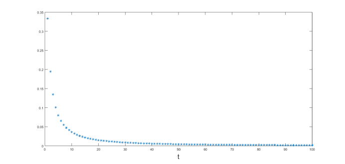
Figure 1.

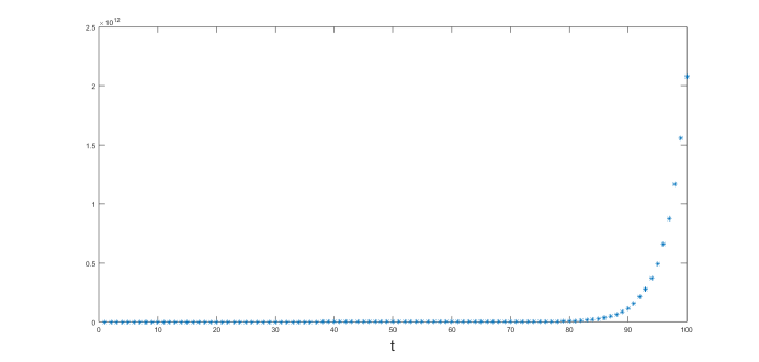
Figure 2.

2.2. Computation of (2.4):

Let $m\in\mathbb{N}_{1}$ and consider the initial value problem associated with (2.2):

$$\begin{cases}\big{(}\nabla^{\nu}_{0*}x\big{)}(t)=\lambda x(t),\quad t\in\mathbb{N}^{m}_{1},\\ x(0)=1.\end{cases}$$ (2.12)

Rewriting the equation in (2.12) using Theorem 1.2 and Theorem 1.3, we have

$$\sum^{t}_{s=1}H_{-\nu-1}(t,\rho(s))x(s)-H_{-\nu}(t,0)x(0)=\lambda x(t),\quad t\in\mathbb{N}^{m}_{1}.$$ (2.13)

Rearranging the terms in (2.13), we obtain

$$(1-\lambda)x(t)+\sum^{t-1}_{s=1}H_{-\nu-1}(t,\rho(s))x(s)=H_{-\nu}(t,0)x(0),\quad t\in\mathbb{N}^{m}_{1}.$$ (2.14)

Denote by $\tilde{x}=[x(1),x(2),\cdots,x(m)]^{T}$. Then, the matrix form of (2.14) is given by

$$\mathcal{L}\tilde{x}=\mathcal{C},$$

where

$$\mathcal{C}=\left(\begin{array}[]{c}H_{-\nu}(1,0)\\ H_{-\nu}(2,0)\\ H_{-\nu}(3,0)\\ \vdots\\ \vdots\\ H_{-\nu}(m-1,0)\\ H_{-\nu}(m,0)\\ \end{array}\right)_{m\times 1}.$$

Since $\mathcal{L}$ is non-singular, the exponential function (2.4) can be computed by the following numerical algorithm:

$$\hat{e}_{\nu}(\lambda,t^{\overline{\nu}})=\mathcal{L}^{-1}\mathcal{C},\quad t\in\mathbb{N}^{m}_{1}.$$

Here $\mathcal{L}=\left[\mathcal{L}_{ij}\right]_{m\times m}$ and $\mathcal{C}=\left[\mathcal{C}_{i}\right]_{m\times 1}$, where

$$\mathcal{L}_{ij}=\begin{cases}1-\lambda,\hskip 55.64821pti=j,\\ 0,\hskip 77.32942pti<j,\\ H_{-\nu-1}(i,\rho(j)),\hskip 10.84006pti>j,\end{cases}$$

and

$$\mathcal{C}_{i}=H_{-\nu}(i,0).$$

Example 4.

Computation of $\hat{e}_{0.5}(-0.5,t^{\overline{0.5}})$ for $t\in\mathbb{N}^{10}_{1}$:

We have

$$\mathcal{C}=\left(\begin{array}[]{c}1\\ 0.5000\\ 0.3750\\ 0.3125\\ 0.2734\\ 0.2461\\ 0.2256\\ 0.2095\\ 0.1964\\ 0.1855\end{array}\right).$$

Then, from Example 1, for $t\in\mathbb{N}^{10}_{1}$,

$$\hat{e}_{0.5}(-0.5,t^{\overline{0.5}})=\mathcal{L}^{-1}\mathcal{C}=\left(\begin{array}[]{c}0.6667\\ 0.5556\\ 0.4907\\ 0.4460\\ 0.4124\\ 0.3857\\ 0.3639\\ 0.3456\\ 0.3299\\ 0.3162\end{array}\right).$$

Example 5.

Computation of $\hat{e}_{0.5}(0.5,t^{\overline{0.5}})$ for $t\in\mathbb{N}^{10}_{1}$:

We have

$$\mathcal{C}=\left(\begin{array}[]{c}1\\ 0.5000\\ 0.3750\\ 0.3125\\ 0.2734\\ 0.2461\\ 0.2256\\ 0.2095\\ 0.1964\\ 0.1855\end{array}\right).$$

Then, from Example 2, for $t\in\mathbb{N}^{10}_{1}$,

$$\hat{e}_{0.5}(0.5,t^{\overline{0.5}})=\mathcal{L}^{-1}\mathcal{C}=\left(\begin{array}[]{c}2\\ 3\\ 4.2500\\ 5.8750\\ 8.0156\\ 10.8516\\ 14.6191\\ 19.6318\\ 26.3067\\ 35.1992\end{array}\right).$$

Example 6.

The graphs of $\hat{e}_{0.5}(0.5,t^{\overline{0.5}})$ and $\hat{e}_{0.5}(-0.5,t^{\overline{0.5}})$ for $t\in\mathbb{N}^{100}_{1}$ are shown in Figures 3 and 4, respectively.

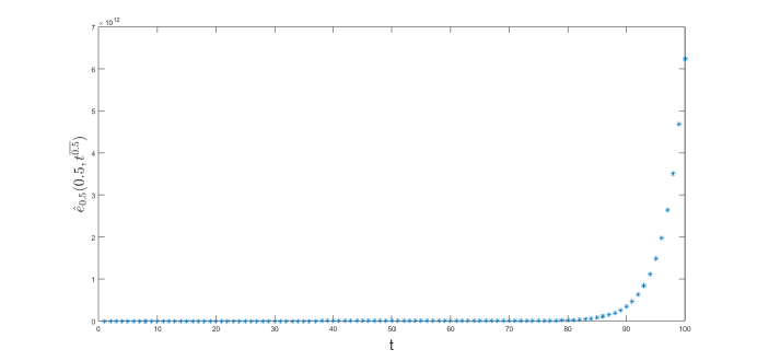
Figure 3.

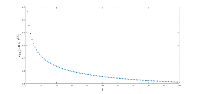
Figure 4.

3. Extensions

The method described in Section 2 can be extended to obtain numerical solutions of initial value problems involving linear non-homogeneous nabla fractional difference equations.

Let $0<\nu<1$ and $m\in\mathbb{N}_{1}$. Consider the initial value problem

$$\begin{cases}\big{(}\nabla^{\nu}_{\rho(0)}u\big{)}(t)=a(t)u(t)+f(t),\quad t\in\mathbb{N}^{m}_{1},\\ \big{(}\nabla^{-(1-\nu)}_{\rho(0)}u\big{)}(0)=u(0)=c,\end{cases}$$ (3.1)

where $a$, $f:\mathbb{N}^{m}_{1}\rightarrow\mathbb{R}$ such that

$$a(t)\neq 1,\quad t\in\mathbb{N}^{m}_{1}.$$

Denote by $\tilde{u}=[u(1),u(2),\cdots,u(m)]^{T}$ and $\mathcal{F}=[f(1),f(2),\cdots,f(m)]^{T}$. Then, the matrix form of (3.1) is given by

$$\mathcal{L}_{1}\tilde{u}=\mathcal{F}-c\mathcal{B},$$

where

is a lower triangular strip matrix. Since $\mathcal{L}_{1}$ is non-singular, the solution of (3.1) can be computed by the following numerical algorithm:

$$u(t)=\mathcal{L}_{1}^{-1}[\mathcal{F}-c\mathcal{B}],\quad t\in\mathbb{N}^{m}_{1}.$$

Replacing the $\nu$-th order Riemann–Liouville nabla fractional difference operator $\nabla^{\nu}_{\rho(0)}$ in (3.1) with the $\nu$-th order Caputo operator $\nabla^{\nu}_{0*}$, the matrix form of the initial value problem

$$\begin{cases}\big{(}\nabla^{\nu}_{0*}u\big{)}(t)=a(t)u(t)+f(t),\quad t\in\mathbb{N}^{m}_{1},\\ u(0)=c,\end{cases}$$ (3.2)

is given by

$$\mathcal{L}_{1}\tilde{u}=\mathcal{F}+c\mathcal{C}.$$

Since $\mathcal{L}_{1}$ is non-singular, the numerical solution of (3.2) can be computed by the following numerical algorithm:

$$u(t)=\mathcal{L}_{1}^{-1}[\mathcal{F}+c\mathcal{C}],\quad t\in\mathbb{N}^{m}_{1}.$$

References

- [1] Abdeljawad, Thabet On delta and nabla Caputo fractional differences and dual identities. Discrete. Dyn. Nat. Soc. 2013 (2013), Art. ID 406910, 12 pp.
- [2] Abdeljawad, Thabet; Atıcı, Ferhan M. On the definitions of nabla fractional operators. Abstr. Appl. Anal. 2012 (2012), Art. ID 406757, 13 pp.
- [3] Acar, Nihan; Atıcı, Ferhan M. Exponential functions of discrete fractional calculus. Appl. Anal. Discrete Math. 7 (2013), no. 2, 343–353.
- [4] Ahrendt, K.; Castle, L.; Holm, M.; Yochman, K. Laplace transforms for the nabla-difference operator and a fractional variation of parameters formula. Commun. Appl. Anal. 16 (2012), no. 3, 317–347.
- [5] Anastassiou, George A., Nabla discrete fractional calculus and nabla inequalities. Math. Comput. Modelling 51 (2010), no. 5-6, 562–571.
- [6] Atıcı, Ferhan M.; Eloe, Paul W., Discrete fractional calculus with the nabla operator. Electron. J. Qual. Theory Differ. Equ. 2009, Special Edition I, no. 3, 12 pp.
- [7] Atici, Ferhan M.; Eloe, Paul W. Linear systems of fractional nabla difference equations. Rocky Mountain J. Math. 41 (2011), no. 2, 353–370.
- [8] Bohner, Martin; Peterson, Allan. Dynamic equations on time scales. An introduction with applications. Birkhäuser Boston, Inc., Boston, MA, 2001.
- [9] Čermák, Jan; Kisela, Tomáš; Nechvátal, Luděk Stability and asymptotic properties of a linear fractional difference equation. Adv. Difference Equ. 2012, 2012:122, 14 pp.
- [10] Elaydi, Saber An introduction to difference equations. Third edition. Undergraduate Texts in Mathematics. Springer, New York, 2005.
- [11] Eloe, Paul; Jonnalagadda, Jaganmohan Mittag-Leffler stability of systems of fractional nabla difference equations. Bull. Korean Math. Soc. 56 (2019), no. 4, 977–992.
- [12] Goodrich, Christopher; Peterson, Allan C. Discrete fractional calculus. Springer, Cham, 2015.
- [13] Gray, Henry L.; Zhang, Nien Fan On a new definition of the fractional difference. Math. Comp. 50 (1988), no. 182, 513–529.
- [14] Jagan Mohan, Jonnalagadda Asymptotic behaviour of linear fractional nabla difference equations. Int. J. Difference Equ. 12 (2017), no. 2, 255–265.
- [15] Jia, Baoguo; Erbe, Lynn; Peterson, Allan Comparison theorems and asymptotic behavior of solutions of discrete fractional equations. Electron. J. Qual. Theory Differ. Equ. 2015, Paper No. 89, 18 pp.
- [16] Kelley, Walter G.; Peterson, Allan C. Difference equations. An introduction with applications. Second edition. Harcourt/Academic Press, San Diego, CA, 2001.
- [17] Kilbas, Anatoly A.; Srivastava, Hari M.; Trujillo, Juan J. Theory and applications of fractional differential equations. North-Holland Mathematics Studies, 204. Elsevier Science B.V., Amsterdam, 2006.
- [18] Miller, Kenneth S.; Ross, Bertram Fractional difference calculus. Univalent functions, fractional calculus, and their applications (Koriyama, 1988), 139–152, Ellis Horwood Ser. Math. Appl., Horwood, Chichester, 1989.
- [19] Nagai, Atsushi An integrable mapping with fractional difference. J. Phys. Soc. Japan 72 (2003), no. 9, 2181–2183.
- [20] Podlubny, Igor. Fractional differential equations. Mathematics in Science and Engineering, 198. Academic Press, Inc., San Diego, CA, 1999.
- [21] Podlubny, Igor Matrix approach to discrete fractional calculus. Fract. Calc. Appl. Anal. 3 (2000), no. 4, 359–386.
- [22] The Anh, Pham; Babiarz, Artur; Czornik, Adam; Niezabitowski, Michal; Siegmund, Stefan Some results on linear nabla Riemann-Liouville fractional difference equations. Math. Methods Appl. Sci. 43 (2020), no. 13, 7815–7824.
- [23] Shobanadevi, N.; Mohan, J. Jagan Stability of linear nabla fractional difference equations. Proc. Jangjeon Math. Soc. 17 (2014), no. 4, 651–657.
- [24] Wu, Guo-Cheng; Baleanu, Dumitru; Luo, Wei-Hua Lyapunov functions for Riemann-Liouville-like fractional difference equations. Appl. Math. Comput. 314 (2017), 228–236.