Propagation of intense few-cycle laser pulse in a telecommunication-type optical fiber: analysis of the error introduced by the unidirectional approximation

Abstract

Propagation of few-cycle laser pulses in optical fiber is investigated beyond the unidirectional approximation. Considered medium parameters include dispersion, Kerr and Raman nonlinearities. High intensities of $\sim 10^{10}\ \textrm{kW}/\textrm{cm}^{2}$ lead to generation of the octave-spanning continuum. The error of the unidirectional approximation is seen in simulations as two pulses propagating forwards and backwards, both remain weak under the considered conditions. Direct analytical estimate of the error is derived and verified numerically. It can be applied to a priory justification of the unidirectional approach.

I Introduction

Theoretical analysis of the evolution of intense few-cycle laser pulses in optical fibers has been a topic of interest in modern optics for the past decades. One of the most frequently used approaches to the simulation of this process relies on the unidirectional approximation, which implies propagation of electromagnetic fields in the forward direction along the waveguide axis Agrawal (2001); Kolesik and Moloney (2004). This reduction of Maxwell’s equations fully ignores fields that propagate backwards. If intensities are low and nonlinearities do not play a role, “forward” and “backward” fields run independently, and the approximation does not introduce any significant error for the homogeneous waveguide. At higher intensities, nonlinear response of the medium becomes more pronounced and coupling between forward and backward waves occurs. In recent papers, Kinsler et al. (2005); Rosanov (2008, 2009) the importance of this coupling is addressed. Despite unavoidable neglect of the backward wave in the unidirectional approach, it provided proper descriptions for the large array of experimental results Bespalov et al. (2002); Agrawal (2001); Akhmanov et al. (1988); Brabec and Ferenc (2000). Several papers are dedicated to the analysis of the limitations of the unidirectional equations Kinsler et al. (2005); Rosanov (2008, 2009). However the resulting conclusions do not seem to allow for a priori estimations of adequacy of the approximation.

In this paper we attempt to cover this gap. We examine, numerically and analytically, the evolution of the fields neglected in the unidirectional approach which is applied to the propagation of intense few-cycle laser pulses in the optical fiber with the non-resonant dispersion and the cubic nonlinearity including electronic and Raman mechanisms. We solve the set of equations for the interaction of the counter-propagating waves and obtain the initial field distributions matched with the nonlinear response of the medium Kinsler et al. (2005); Konev and Shpolyanskiy (2014). Profiles of forward and backward waves are presented for the normal and anomalous dispersion including the regime of significant self-steepening. Without the mentioned matching a reflected wave appears due to the form of the boundary conditions Kinsler et al. (2005); Konev and Shpolyanskiy (2014). A simple analytical estimate of its amplitude is obtained. It shows that the reflected wave is weak in transparent media without interfaces. The amplitude is proportional to the amplitude of the forward wave and has the order of magnitude equal to the nonlinear refractive index divided by the linear refractive index. The equation for backward wave produces an additional field that propagates forward together with the forward wave, which is always neglected in the unidirectional approximation. It has the same order of amplitude as the non-matched reflected wave.

II Equations

We consider the propagation of linearly polarized few-cycle femtosecond pulses in a single-mode telecommunication-type fused silica fiber. The presented theoretical approach is not restricted to this specific case and can be applied to other transparent optical media with non-resonant dispersion and nonlinearity. Transverse field distribution defined by the mode structure is assumed to be invariable during the pulse propagation. It allows for reduction of Maxwell’s equations in non-magnetic optical waveguide to the scalar second-order wave equation for the spectrum of electrical field, which can be written in the following form Kinsler et al. (2005); Boyd (2008):

$$\partial_{z}^{2}G=-k^{2}(\omega)G-k^{2}(\omega)N_{\omega}(E),$$ (1)

$$N_{\omega}=\dfrac{4\pi F[P_{\textrm{NL}}(E)]}{n^{2}(\omega)},$$ (2)

where $N_{\omega}(E)$ is the spectral representation of the nonlinear operator applied to the field; $P_{\textrm{NL}}(E)$ is the nonlinear medium response; $G=F[E]$ is the field spectrum; $k(\omega)=\omega n(\omega)/c$ is the propagation constant; $n(\omega)$ is the refractive index; $\omega$ is the frequency; $c$ is the velocity of light in vacuum; $z$ is the propagation coordinate along waveguide axis; $t$ is the time coordinate; $F$ denotes the Fourier transform:

$$G(z,\omega)=F[E(z,t)]=\int_{-\infty}^{+\infty}E(z,t)\exp(i\omega t)\textrm{d}t.$$ (3)

As it was shown by a number of authors Kinsler et al. (2005); Kinsler (2010); Ferrando et al. (2005), one can easily factorize equation (1) after transformation into the wave vector space (see e.g. Appendix A in Kinsler (2010)). If the space frequency is denoted as $\eta$, this yields two terms: $\eta-k$ and $\eta+k$, corresponding to the “forward” ($E_{+}$) and “backward” ($E_{-}$) waves, respectively:

$$E=E_{+}+E_{-},$$ (4)

$$\begin{dcases}\partial_{z}G_{+}=+ik(\omega)G_{+}+\dfrac{1}{2}ik(\omega)N_{\omega}(E_{+}+E_{-}),\\ \partial_{z}G_{-}=-ik(\omega)G_{-}-\dfrac{1}{2}ik(\omega)N_{\omega}(E_{+}+E_{-}).\end{dcases}$$ (5)

By differentiating with respect to $z$ and summing up Eqs. (5) it is easy to see that the total field (4) satisfies (1).

If $E_{-}$ is ignored in (5), only the first equation for $E_{+}$ remains, which is essentially the same as the unidirectional pulse propagation equation Tani et al. (2014); Kolesik and Moloney (2004).

III Medium response

Let us now complete the set of equations (5) with a detailed model of the medium response. The necessary ingredients in the field of intense few-cycle pulses are the linear dispersion and the nonlinearity of the medium. As we consider propagation distances less than $2\ \textrm{mm}$, the linear absorption of fused silica is insignificant and can be ignored.

Non-resonant dispersion of the refractive index of fused silica in its range of transparency can be described with high accuracy by the Sellmeier’s formula Agrawal (2001):

$$n(\omega)^{2}=1+\sum_{i}\dfrac{B_{i}\omega_{i}^{2}}{\omega_{i}^{2}-\omega^{2}},$$ (6)

where $i=\{1,2,3\}$; $B_{1}=0.6961663$, $B_{2}=0.4079426$ and $B_{3}=0.8974794$ are the amplitudes of the resonances; $\omega$ is the frequency of the field; $\omega_{i}=2\pi c/\lambda_{i}$ are the resonant frequencies, $\lambda_{1}=0.0684043\ \mu m$, $\lambda_{2}=0.1162414\ \mu m$, $\lambda_{3}=9.896161\ \mu m$ are the resonant wavelengths of the medium.

The two dominant components for the nonlinear interaction of the fused silica with the field of intense ultrashort pulses are the instantaneous electronic cubic nonlinearity and the low-inertial cubic Raman nonlinearity. The standard phenomenological model described in Platonenko et al. (1966); Jalali et al. (2006) incorporates both of them:

$$\begin{cases}P_{\textrm{NL}}=\chi_{3,\textrm{e}}E^{3}+\chi_{3,\textrm{ev}}RE,\\ \partial_{t}^{2}R+\dfrac{1}{T_{\textrm{v}}}\partial_{t}R+\omega_{\textrm{v}}^{2}R=\gamma E^{2}.\end{cases}$$ (7)

Here $R$ is the amplitude of the molecular oscillations, which describes connection between the electrical field of the pulse and the oscillation of the molecules in the medium; $T_{\textrm{v}}$ is the relaxation time; $\omega_{\textrm{v}}$ is the vibrational frequency of molecules; $\chi_{3,\textrm{e}}$ and $\chi_{3,\textrm{ev}}$ are the Kerr and Raman cubic nonlinear susceptibilities, respectively; $\gamma$ is the coefficient that characterizes the relation between the Kerr and Raman responses. In (7), $R$ and its first time derivative are zero before the pulse appears. The nonlinear refractive index coefficient $n_{2}$ in CGS units can then be expressed as the sum of components related to $\chi_{3,\textrm{e}}$ and $\chi_{3,\textrm{ev}}$ respectively as Akhmanov et al. (1988); Kozlov et al. (1999):

$$n_{2}=n_{2,\textrm{e}}+n_{2,\textrm{ev}},\ n_{2,\textrm{e}}=\dfrac{3\pi\chi_{3,\textrm{e}}}{n(\omega_{0})},\ n_{2,\textrm{ev}}=\dfrac{2\pi\gamma\chi_{3,\textrm{ev}}}{\omega_{\textrm{v}}^{2}n(\omega_{0})}.$$ (8)

For fused silica, nonlinear refractive indices are estimated to have values $\tilde{n}_{2,\textrm{e}}=2.9\times 10^{-20}m^{2}/W$ and $\tilde{n}_{2,\textrm{ev}}=7.25\times 10^{-21}m^{2}/W$ in SI units Agrawal (2001); Kozlov et al. (1999). Here, $\omega_{0}$ is the central frequency of radiation spectrum.

IV Initial field distribution

The method we use requires the knowledge of the full time profile of the field at a given point on the $z$ axis. This requirement is natural for the so-called $z$-propagated equations, such as the set (5). Nonlinear and dispersive effects are conveniently covered by this type of equations. While time spectra can be observed directly in experiments, it is essential that these equations describe their evolution. Another important aspect is that the dispersion response of transparent media is represented naturally (and in the simplest form!) in the frequency domain. It makes the approach very productive and provides the explanation for experimental results Bespalov et al. (2002); Agrawal (2001); Akhmanov et al. (1988); Brabec and Ferenc (2000). However, the process of injection of a given time profile into the fiber is not addressed, which introduces difficulties with physical interpretation of the problem setup Rosanov (2016). Generically, both forward and backward waves have to be known at the input and output sections of the waveguide to form a certain profile. The forward wave is assumed to be given at the input, but the backward wave is usually unknown there, which breaks the symmetry. This issue is immanent for $z$-propagated equations and cannot be avoided. However, in the case of the unidirectional approximation this limitation is less pronounced because it is shaded by a stronger assumption of insignificance of the backward wave. If we consider equations for the forward and backward waves and set the initial distribution of the latter to be zero at $z=0$, the problem formulation becomes similar to that for the unidirectional approximation. It allows us to reveal the difference between the second-order wave equation (1) written in form of (5) and the unidirectional approximation.

As it was shown in our previous paper Konev and Shpolyanskiy (2014), a backward-propagating field appears in the beginning of the simulation in such a setup. The calculated backward wave consists of two sub-pulses propagating in opposite directions. The part propagating backward $E_{-}^{\textrm{left}}$ does not change its spectral form after its formation and separation from the initial pulse. The other part $E_{-}^{\textrm{right}}$ is tightly coupled with the forward wave, its evolution is induced by the forward wave during the whole simulation process.

We examine this behavior by looking at the simplified set of equations for the forward and backward waves, that describes their propagation over the distances of just a few wavelengths. The forward wave does not evolve over distances that are so short, it only propagates with the group velocity. Therefore, higher order dispersion terms can be ignored as well as the nonlinearity. As for the backward wave, its presence in the considered setup comes from the nonlinear term of the original set, which therefore has to be included in the resulting equation together with the backward move with the group velocity. It gives the following simplified set of equations:

$$\begin{cases}\partial_{z}E_{+}=-\dfrac{1}{V_{\textrm{g}}}\partial_{t}E_{+},\\ \partial_{z}E_{-}=+\dfrac{1}{V_{\textrm{g}}}\partial_{t}E_{-}+\dfrac{2\pi}{cn(\omega_{0})}\partial_{t}P_{\textrm{NL}}(E_{+}),\end{cases}$$ (9)

where $V_{\textrm{g}}=n_{\textrm{g}}/c$ is the group velocity and $n_{\textrm{g}}$ is the group refractive index, both calculated at $\omega_{0}$. The forward wave in this case is just the solution of the transport equation:

$$E_{+}(z,t)=E_{+}(0,t-z/V_{\textrm{g}})=E_{0+}(t-z/V_{\textrm{g}}),$$ (10)

where $E_{0+}$ is the initial distribution of the forward wave. The backward wave can also be written out analytically as the sum of parts propagating in negative (left) and positive (right) directions of the $z$ axis:

$$E_{-}(z,t)=E_{-}^{\textrm{left}}(z,t)+E_{-}^{\textrm{right}}(z,t),$$ (11)

$$E_{-}^{\textrm{left}}(z,t) =E_{0-}(t+z/V_{\textrm{g}})+$$ (12)

$$+\dfrac{\pi}{n_{0}n_{\textrm{g}}}P_{\textrm{NL}}[E_{0+}(t+z/V_{\textrm{g}})],$$

$$E_{-}^{\textrm{right}}(z,t)=-\dfrac{\pi}{n_{0}n_{\textrm{g}}}P_{\textrm{NL}}[E_{+}(z,t)],$$ (13)

where $n_{0}=n(\omega_{0})$.

The presence of the forward-running part (13) in the backward wave looks surprising at first, but it can be justified both analytically and numerically. From (13) we see that this part is fully induced by the forward wave, runs along with it and has the opposite sign. The backward-running part (12) includes two terms. The first term represents the initial distribution of the backward wave moving with the group velocity in the negative $z$ direction. The second one is induced by the forward wave. These terms eliminate each other if we take the initial distribution of the form:

$$E_{0-}(t)=-\dfrac{\pi}{n_{0}n_{\textrm{g}}}P_{\textrm{NL}}[E_{0+}(t)].$$ (14)

This is the so-called matched distribution Kinsler et al. (2005). Note that the nonlinear response appears in (12), (13) without concretization of its form. For the nonlinear response (7) the analytical estimate of the amplitude of the backward wave compared to the amplitude of the forward wave is:

$$\Gamma=\left|\dfrac{E_{-}^{\textrm{right}}}{E_{+}}\right|=\left|\dfrac{\pi P_{\textrm{NL}}(E_{0+})}{n_{0}n_{\textrm{g}}E_{0+}}\right|=\left|\dfrac{n_{2,\textrm{e}}E_{0+}^{2}}{3n_{\textrm{g}}}+\dfrac{\omega_{\textrm{v}}^{2}n_{2,\textrm{ev}}R(E_{0+})}{2\gamma n_{\textrm{g}}}\right|.$$ (15)

$R(E_{0+})$ can be obtained analytically or numerically from the second equation in (7). Note, that (15) depends only on the properties of the medium and the initial distribution of the forward wave, hence it can be used for the a priori estimation of the expected error originating from the assumption of the unidirectional propagation.

V Simulation results

We solve system (5) numerically with Fourier split-step method Agrawal (2001). Each step $\Delta z$ is split into 2 sub-steps. First nonlinearity is accounted for in the time domain using the Crank-Nicolson scheme with internal iterations until convergence is reached. Next, the dispersive effects are calculated in the frequency domain. The error is analyzed by doubling the number of steps in $z$ and $t$. The conservation of the total energy is checked as well.

For the model of the initial distribution of a few-cycle forward pulse we take Gaussian profile in the form:

$$E_{0+}(t)=E_{\textrm{max}}\exp(-2t^{2}/T_{0}^{2})\sin(\omega_{0}t),$$ (16)

where $E_{\textrm{max}}$ is the amplitude of the pulse; $\omega_{0}=2\pi c/\lambda_{0}$, $\lambda_{0}$ is the central wavelength; $\Delta\tau_{0}=NT_{0}$ is the duration; $T_{0}=\lambda_{0}/c$ is the period; $N$ is the number of oscillations and $I$ is the peak intensity.

First we simulate the propagation of the pulse under the conditions of normal group dispersion. The pulse parameters are $\lambda_{0}=780\ \textrm{nm}$, $\Delta\tau_{0}=6T_{0}=15.6\ \textrm{fs}$ and $I=2\times 10^{10}\ \textrm{kW}/\textrm{cm}^{2}(I[\textrm{kW}/\textrm{cm}^{2}]=(3n(\omega_{0})/8\pi)(E_{\textrm{max}})^{2}[CGS]$ Akhmanov et al. (1988)). The backward wave is matched to the nonlinear response of the medium at $z=0$ using (14) in order to avoid artificial self-reflection.

The pulse propagation over the first 5 wavelengths is visualized in Fig. 1. The forward and backward waves are depicted by the thin and thick curves, respectively. One can see both the $E_{-}^{\textrm{left}}$ and $E_{-}^{\textrm{right}}$ parts of the backward wave. The part $E_{-}^{\textrm{right}}$ that propagates to the right along with the forward pulse agrees very well with (13) obtained from the simplified system (9); the difference is indistinguishable on the plot. The amplitude of this numerically calculated field is approximately $2.7\times 10^{-3}E_{\textrm{max}}$, which agress with the estimate (15). The part $E_{-}^{\textrm{left}}$ is $\sim 25$ times weaker than $E_{-}^{\textrm{right}}$, its profiles are given scaled-up in insets. At $z=0$ $E_{-}^{\textrm{left}}$ is zero, but it is fully formed over the first 5 wavelengths and moves to the left. The simplified system (9) predicts the absence of $E_{-}^{\textrm{left}}$ for the matched conditions. However, in the system (5) higher order dispersion terms originating from (6) are significant, hence the full matching requires consideration of their contribution to the refractive index. They are ignored in (9), and we attribute the very weak, but non-zero $E_{-}^{\textrm{left}}$ to the neglect of dispersion effects in derivation of the matching condition (14). It is confirmed by the fact that $E_{-}^{\textrm{left}}$ does not grow after the initial generation and its spectral density does not vary as will be shown below.

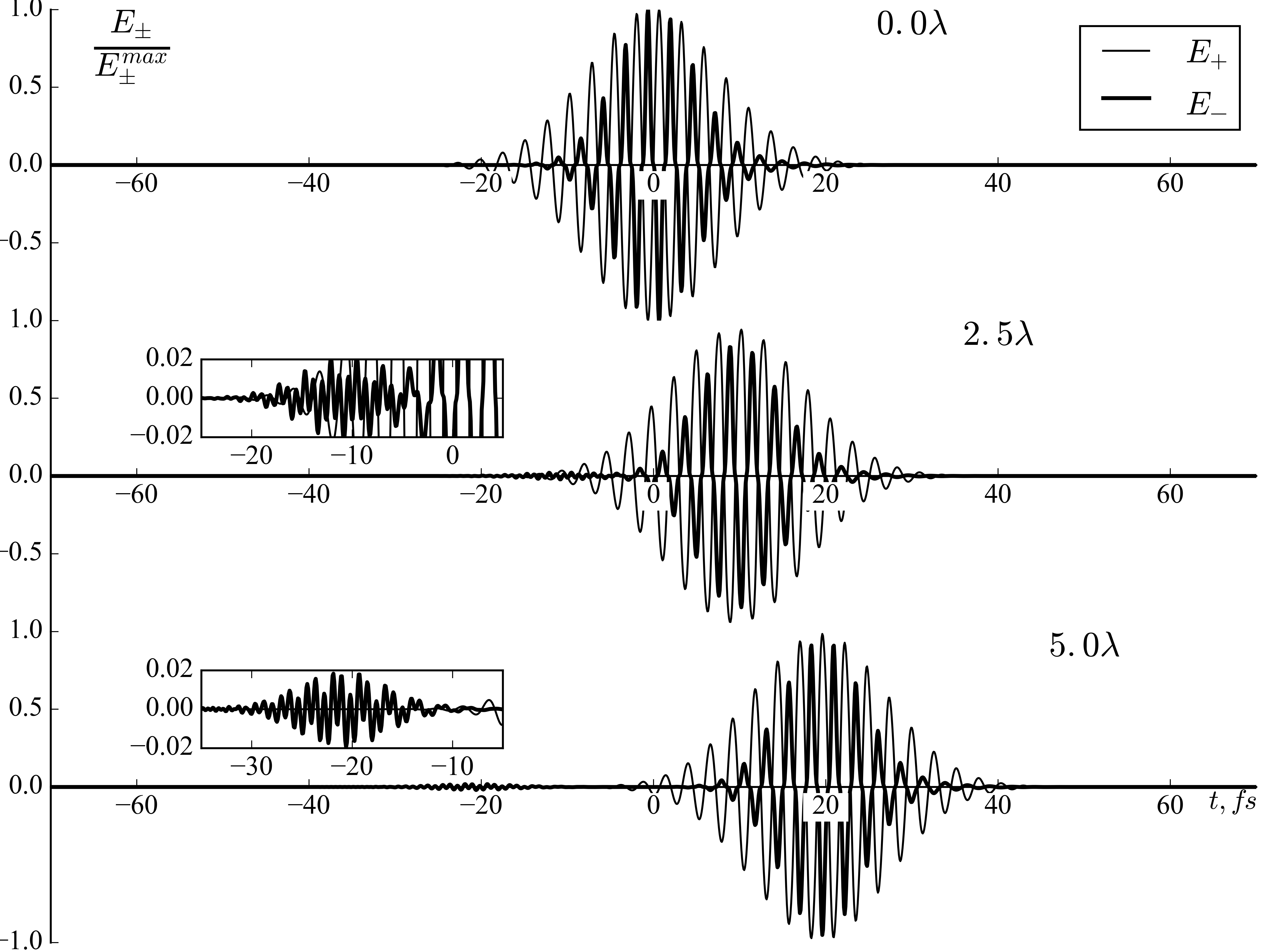
Figure 1: Normalized field profiles of the forward $E_{+}$ and backward $E_{-}$ waves at the initial stage of the propagation. Input parameters of the forward wave: central wavelength $\lambda_{0}=780\ \textrm{nm}$, duration $\Delta\tau_{0}=15.6\ \textrm{fs}$ and intensity $I=2\times 10^{10}\ \textrm{kW}/\textrm{cm}^{2}$. The backward wave at $z=0$ is taken in the form of (14) to be matched with the nonlinear response of the medium. Ratio of the field amplitudes $E_{-}^{\textrm{max}}/E_{+}^{\textrm{max}}\approx 2.7\times 10^{-3}$. The part of the backward wave propagating backwards is given scaled-up in insets.

Distributions of $E_{+}$ and $E_{-}$ at further distances $z$ up to $0.9\ \textrm{mm}$ can be seen in Fig. 2. Limits of the $t$ axis in the plots are adjusted to depict fields propagating forwards, so that $E_{-}=E_{-}^{\textrm{right}}$ in those $(z,t)$ regions. The forward pulse exhibits considerable broadening and shaping under the combined effect of the nonlinearity and dispersion with appearance of a chirp typical for the normal dispersion: higher frequencies appear at the tail of the pulse. Clearly, the numerical solution does not satisfy the simplified system (9). However, the field $E_{-}^{\textrm{right}}$ is not only fully defined by the forward field $E_{+}$, but, surprisingly, remains related to the latter with (13). The field $E_{-}^{\textrm{left}}$ running to the left is beyond the visualized $(z,t)$ regions. Formed by $z=5\lambda_{0}$ (see insets in Fig. 1), this field changes slowly under the influence of the dispersion. Normalized spectral densities $G_{+}$, $G_{-}^{\textrm{right}}$, and $G_{-}^{\textrm{left}}$ of $E_{+}$, $E_{-}^{\textrm{right}}$, and $E_{-}^{\textrm{left}}$, respectively, are shown in Fig. 3. It can be seen that $E_{-}^{\textrm{left}}$ does not vary from $z=0.3\ \textrm{mm}$ to $z=0.9\ \textrm{mm}$, i.e. it is not affected by the nonlinearity. Furthermore the spectrum of the forward pulse is super-broadened, its main part is asymmetric ranging from $\sim 0.4\omega_{0}$ to $\sim 2\omega_{0}$ and includes triple frequencies that are inherent to the cubic nonlinearity. The spectrum $G_{-}^{\textrm{right}}$ is even broader due to (13), it reaches the fifth harmonic.

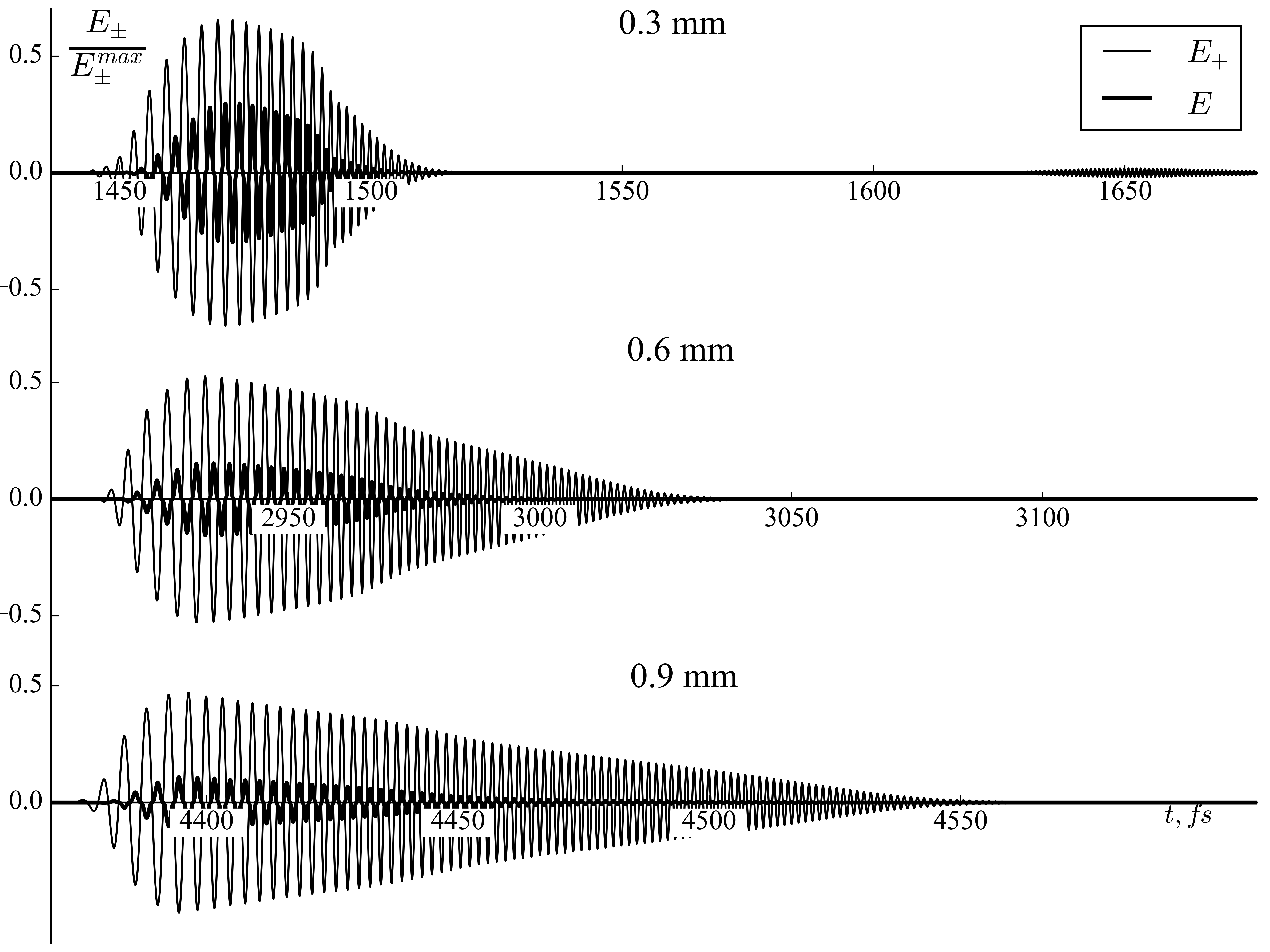
Figure 2: Normalized field profiles of the forward and backward waves after propagation over the distances of $z=0.3,\ 0.6$ and $0.9\ \textrm{mm}$. Parameters are identical to those in Fig. 1.

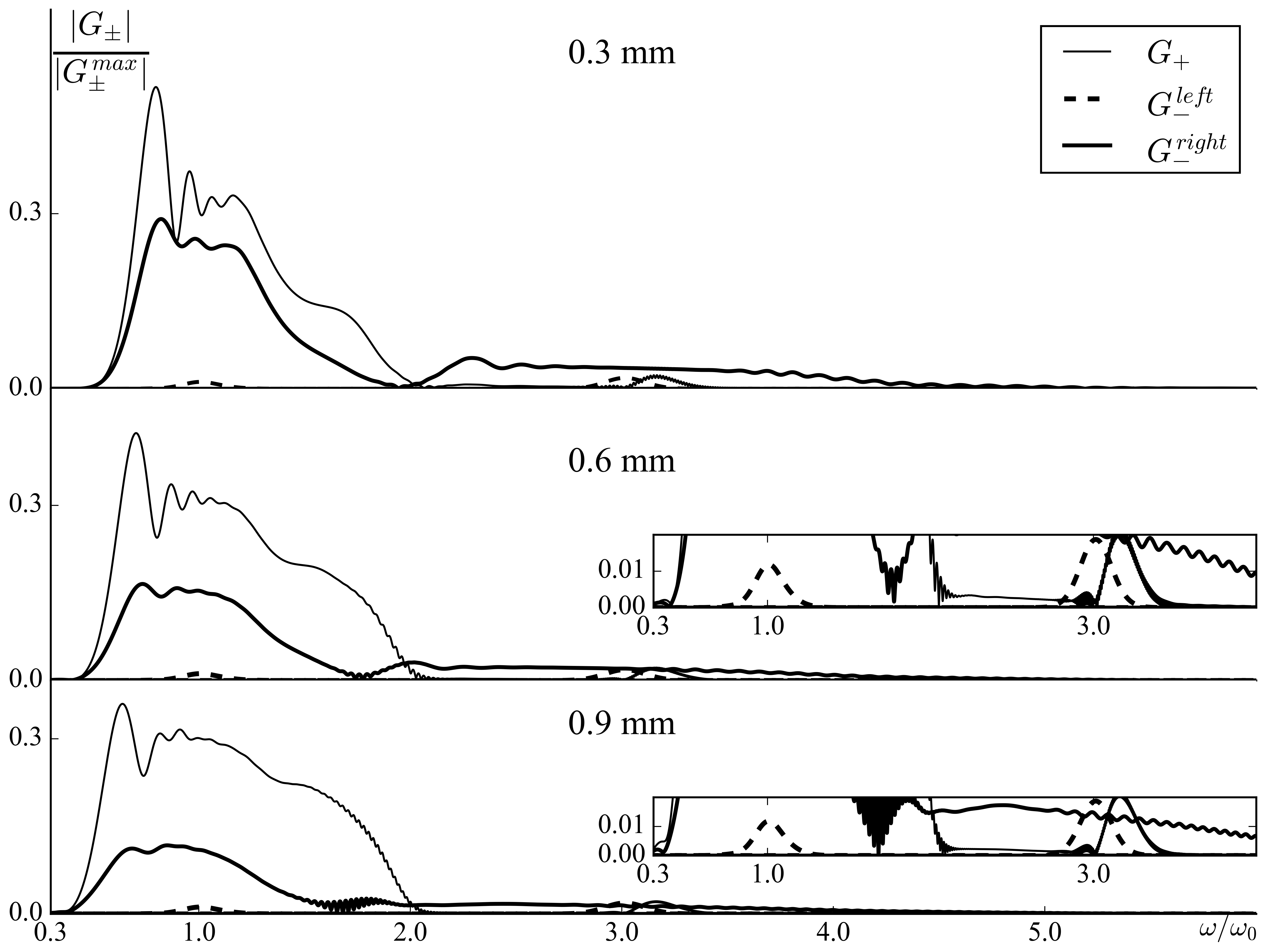
Figure 3: Normalized spectral densities of the fields of forward and backward waves after propagation over the distances of $z=0.3,\ 0.6$ and $0.9\ \textrm{mm}$. Parameters are identical to those in Fig. 1.

It is well known that a pulse that propagates under conditions of anomalous dispersion and cubic nonlinearity experiences strong steepening Trippenbach and Band (1998). For few-cycle pulses the duration of the tail can become even shorter than one field cycle Shpolyanskiy et al. (2003). The adequacy of unidirectional approximation for such highly nonlinear scenario is questionable, because an area appears of extremely localized light field. In order to investigate possible features of the field evolution introduced by inclusion of the backward wave into consideration we simulated the propagation of the pulse with central wavelength of $1500\ \textrm{nm}$, duration of $50\ \textrm{fs}$ and intensity of $5\times 10^{9}\ \textrm{kW}/\textrm{cm}^{2}$. Initial distribution of the backward wave was, as before, matched with the nonlinear response of the medium according to (14). The calculated fields and spectra of the forward and backward waves at distances $z$ of $0.0,\ 1.25,\ 1.5$ and $1.85\ \textrm{mm}$ are given in Fig. 4 and 5, respectively. As shown in Fig. 6, by the distance of $1.6\ \textrm{mm}$ the tail of the forward pulse is considerably steepened. Extreme spectral broadening with splitting into lower and high-frequency parts is observed, as is typical for the anomalous dispersion Trippenbach and Band (1998). Generation of intense third harmonics is clearly seen in Fig. 5. The width of spectral supercontinuum exceeds 1.5 octaves. The pulse tail is formed from higher-frequency components and includes features varying sharply in the time scale of a period of the initial central frequency (see Fig. 6). The forward-propagating part of the backward wave is again fully defined by the forward pulse and related to it via the analytic expression (13). Its spectrum reaches the fifth harmonic. However, even this regime does not lead to generation of the reflected wave as can be seen from Fig. 5: $G_{-}^{\textrm{left}}$ does not vary from $z=1.25\ \textrm{mm}$ to $z=1.85\ \textrm{mm}$. The amplitude of $E_{-}^{\textrm{left}}$ is about 82 times smaller than the amplitude of $E_{-}^{\textrm{right}}$, which in turn is $\sim 0.8\times 10^{-3}$ of $E_{+}$.

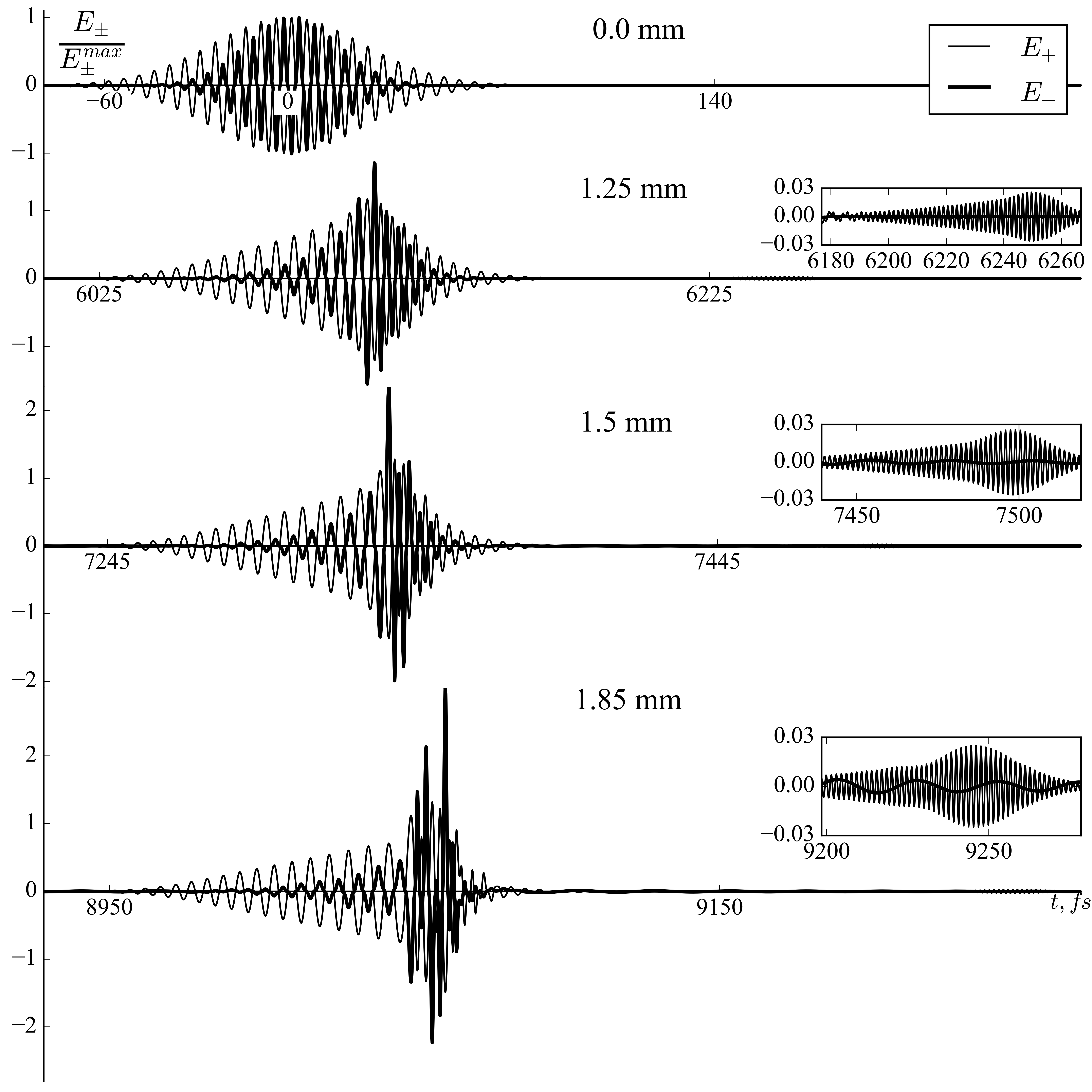
Figure 4: Field distributions of the forward and backward waves of the pulse with intensity $I=5\times 10^{9}\textrm{kW}/\textrm{cm}^{2}$ after propagation over the distance of $z=0.0,\ 1.25,\ 1.5$ and $1.85\ \textrm{mm}$ under conditions of anomalous dispersion, $E_{-}^{\textrm{max}}/E_{+}^{\textrm{max}}\approx 0.8\times 10^{-3}$.

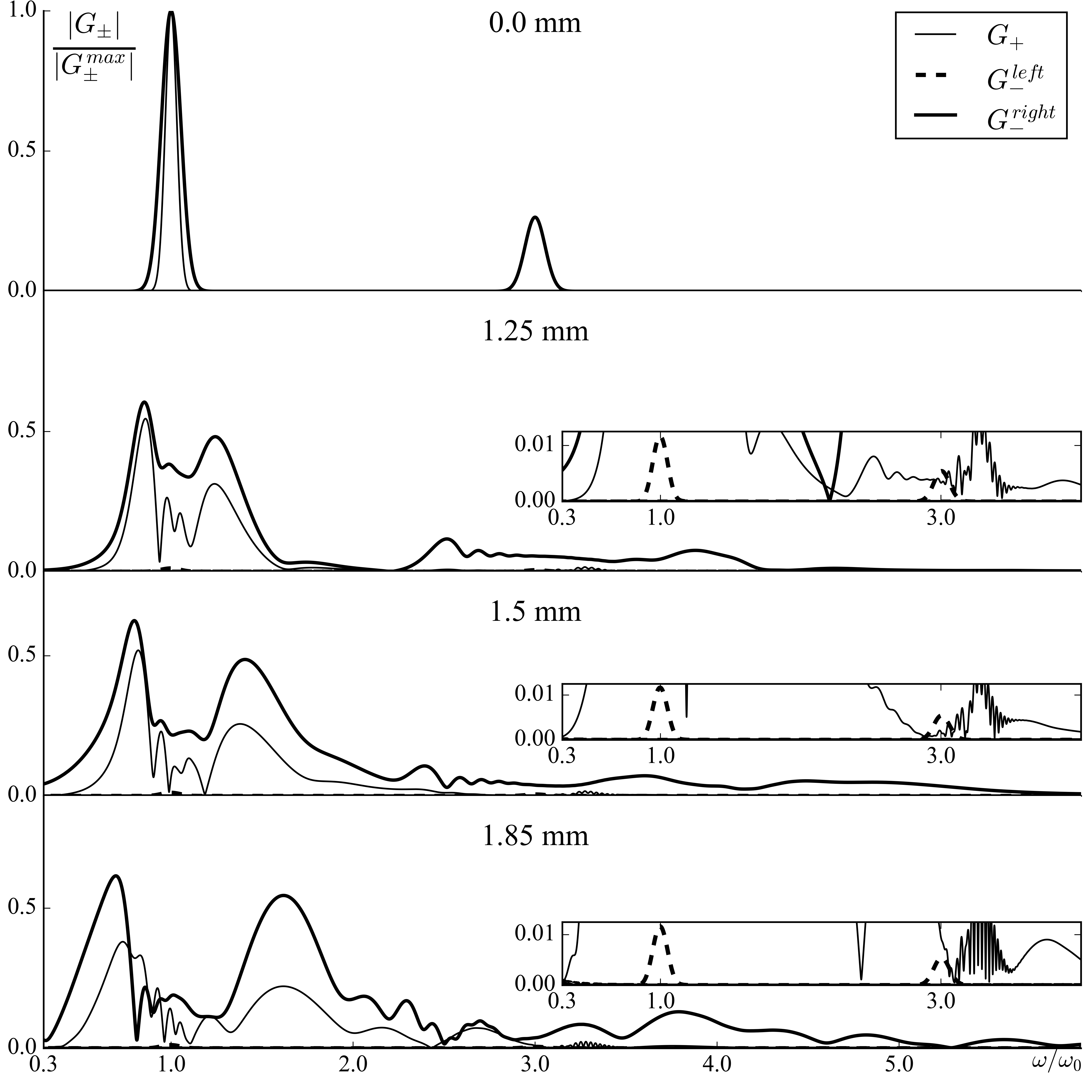
Figure 5: Normalized spectral densities of the fields of forward and backward waves after propagation over the distances of $z=0.0,\ 1.25,\ 1.5$ and $1.85\ \textrm{mm}$. Parameters are identical to those in Fig. 4.

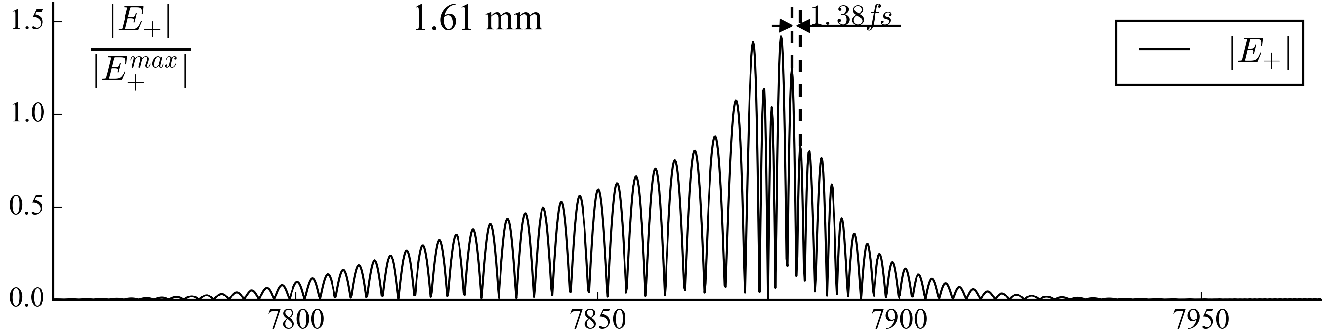
Figure 6: Density of the forward wave propagated over the distance of $1.61\ \textrm{mm}$ with extremely steepened tail.

VI Conclusion

We have simulated forward and backward waves of few-cycle pulses propagating in single-mode regime in telecommunication-type fused-silica fiber using the $z$-propagated approach. Scenarios of pulse evolution at intensities of the order of $10^{10}\ \textrm{kW}/\textrm{cm}^{2}$ are considered for the normal and anomalous dispersion range of the fiber. Under the combined action of the cubic nonlinearity and dispersion the forward wave experiences tremendous changes with generation of octave-spanning spectrum. In time domain, a sharp steepening of the pulse tail is observed in anomalous-dispersion regime.

The structure of the field which is ignored in the unidirectional approximation is investigated analytically and numerically. It includes two parts: one part propagates in the forward direction along with the forward wave, the other one propagates backwards. It is shown that the former can be calculated from the forward wave via the simple expression (13) instead of numerical solution of the equation for the backward wave. If the matched initial distribution (14) is applied, the field propagating backwards becomes considerably weaker than the forward-running part. We believe that it is not zero since we ignored dispersion effects in derivation of the matching condition (14).

In our numerical experiments, the backward wave remains weak and does not affect the forward wave. It validates the usage of the unidirectional approximation for such setups at intensities up to the order of $10^{10}\ \textrm{kW}/\textrm{cm}^{2}$. The estimate of the amplitude of the backward wave given by (15) is confirmed by numerical results and can be used for a priori justification of the application of the unidirectional approach. In the considered scenarios, this amplitude was less than $3\times 10^{-3}$ of the amplitude of the forward wave.

Starting this work, we were going to reveal disadvantages of the unidirectional approximation. But our investigations only confirm that it is a brilliant approach for the nonlinear optics in transparent media with non-resonant dispersion and nonlinearity. The main drawback is the inability to describe injection of a given field profile into the waveguide which is immanent to $z$-propagated equations. Neglect of the backward wave does not lead to wrong results for the forward wave, but simplifies equations significantly. Instead of the second-order wave equation (1) or equivalent system of two coupled equations (5) one gets a single first-order equation. It is solved naturally in a frame running with the group velocity of the forward pulse, which reduces the necessary time window dramatically and provides a huge economy of computational resources in numerical simulations.