A Simple Generic Model of Cellular Polarity Alignment:
Derivation and Analysis

Abstract

Ordered polarity alignment of a cell population plays a vital role in biology, such as in hair follicle alignment and asymmetric cell division. Here, we propose a theoretical framework for the understanding of generic dynamical properties of polarity alignment in interacting cellular units, where each cell is described by a reaction-diffusion system and the cells further interact with one another through their proximal surfaces. The system behavior is shown to be strongly dependent on geometric properties such as cell alignment and cell shape. Using a perturbative method under the assumption of weak coupling between cells, we derive a reduced model in which each cell is described by just one variable, the phase. The reduced model resembles an XY model but contains novel terms that possesses geometric information, which enables the understanding of the geometric dependencies as well as the effects of external signal and noise. The model is simple, generic, and analytically and numerically tractable, and is therefore expected to facilitates studies on cellular polarity alignment in various nonequilibrium systems.

Introduction–. Spatially ordered patterns are ubiquitous in nature and have been of central importance in various disciplines Cross and Hohenberg (1993); Meinhardt and Gierer (2000); Nakao and Mikhailov (2010). This work is concerned with dynamical alignment of polarity in interacting cellular units. Spin is a prototypical example of a polar unit. Spins are spatially aligned to magnetize through spin-spin interaction and their response to an external field, as described by, e.g., Ising and XY models Kosterlitz (1974). The present work focuses on nonequilibrium systems, including chemical and biological systems. Polarity can be regarded as an asymmetric distributions in chemical species within a cellular unit. Polarity is of great importance in biology because it is essential for, e.g., cell movement and oriented cell division Devenport (2014). Moreover, cell polarity is often spatially coordinated across a cell population for functional reasons. A well-known example in biology is planar cell polarity (PCP), which refers to the coordinated alignment of cell polarity across planar tissue. This underlies the alignment of, e.g., hair follicles and cilia positioning Devenport (2014). So far, several mathematical models have been proposed to address the effects of various factors on polarity alignment including cell shape, external signal, and noise. Some studies employ detailed models, where each cell is described by a reaction-diffusion system and these cells are further coupled through proximal membranes Amonlirdviman et al. (2005); Burak and Shraiman (2009). Some studies employ simple phenomenological models similar to models for magnetizationAigouy et al. (2010); Ayukawa et al. (2014), which is a reasonable approach because the cell alignment process phenomenologically resembles magnetization. The former contains many free parameters and is too complicated to provide general understandings. On the other hand, in the latter, models are rather arbitrary and may lack essential dynamical features.

In the present Letter, the generic dynamical properties of cell polarity alignment are examined, through deriving a reduced model for coupled reaction-diffusion systems using a perturbative method. In our reaction-diffusion model, each cell is described by a reaction-diffusion system and the cells mutually inhibit one another through their proximal surfaces. Its reduced model, referred to as a phase model, is drastically simple yet reasonably approximates the original reaction-diffusion model when cells are weakly coupled. Our phase model resembles the XY model but includes novel terms representing geometric information such as cell shape and the relative position between neighboring cells. By taking advantage of its tractability, essential dynamical properties including the effects of cell shape, external signal, and noise are analytically clarified, which has only been studied numerically in previous studies using detailed models Amonlirdviman et al. (2005); Burak and Shraiman (2009); Aigouy et al. (2010). Our study bridges the gap between detailed and phenomenological models, and is expected to facilitate the study of polarity dynamics in various nonequilibrium systems.

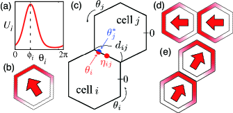
Figure 1: (Color online). (a) Unimodal distribution on the surface of a cell and polarity orientation. (b) Color scale representation and polarity orientation corresponding to (a). (c) Model description. (d,e) Examples of polarity patterns of two coupled cells with different cell alignments.

Model–. Our entire system is composed of a population of cells aligned in two-dimensional space. Reaction-diffusion dynamics of each cell take place on the one-dimensional surface of their perimeter $2\pi$, and the cells further interact with one another through the proximal surfaces between them. Each cell obeys

$$\frac{\partial}{\partial t}\bm{X}_{i} =\bm{F}(\bm{X}_{i})+\hat{D}\frac{\partial^{2}\bm{X}_{i}}{\partial\theta_{i}^{2}}+\epsilon\sum_{j\in A(i)}\bm{H}_{ij},$$ (1)

where $\bm{X}_{i}=\bm{X}_{i}(\theta_{i},t)$ ($i=1,\ldots,N$) denotes the concentration of chemical species at time $t$ and the position $\theta_{i}$ ($0\leq\theta_{i}<2\pi$) on the surface of each cell, $\bm{F}$ describes the local reaction dynamics, $\hat{D}$ is the diagonal matrix consisting of diffusion coefficients, $A(i)$ is the set of cells adjacent to cell $i$, $\bm{H}_{ij}$ describes intercellular interaction, and $\varepsilon$ is the coupling strength. As will be described later, external signal and noise may also be considered. Note that $\bm{H}_{ij}$ is generally a functional of $\bm{X}_{i}(\theta_{i},\cdot)$ and $\bm{X}_{j}(\theta_{j},\cdot)$. Each cell is assumed to exhibit a unimodal distribution for $\varepsilon=0$; i.e., polarity is spontaneously formed. The polarity orientation of cell $i$ is defined by the $\theta_{i}$ value at which the first component of $\bm{X}_{i}(\theta_{i},t)$, denoted by $U_{i}(\theta_{i},t)$, takes its maximum [see Figs. 1(a,b)].

As examples, we consider two models: (a) the real Ginzburg-Landau equation (GLE) and (b) the activator-inhibitor model. Both of these models have two variables, denoted by $\bm{X}_{i}=(U_{i},V_{i})$ (see Supplemental Material A for details). The former is a long-wave amplitude equation, which is widely used to describe various systems near the onset of instability. The latter is a reaction-diffusion model, describing biological pattern formation Koch and Meinhardt (1994). In these models, given appropriate initial conditions, $\bm{X}_{i}$ exhibits a stationary unimodal distribution within individual cells for $\varepsilon=0$, thus they are suitable as dynamical models describing cell polarity.

Intercellular interaction is assumed to occur at every contact point of the neighboring cells. Geometric parameters are defined as shown in Fig. 1(c), where $\eta_{ij}$ and $d_{ij}$ are the midpoint and the length of the proximal surface between cell $i$ and $j$, respectively, and $\theta_{j}^{*}$ is the position in cell $j$ facing $\theta_{i}$ in cell $i$. The interaction function is given as

$$\bm{H}_{ij}=(S_{ij}(\theta_{i}-\eta_{ij})\left\{U_{i}(\theta_{i})-U_{j}(\theta_{j}^{*})\right\},0).$$ (2)

where $S_{ij}(\theta_{i}-\eta_{ij})$ desribes the position of contact, given as $S_{ij}(\theta)=1$ for $|\theta|\leq\frac{d_{ij}}{2}$ and $S_{ij}(\theta)=0$ otherwise. When the cell has a regular hexagonal shape, which is assumed henceforth unless otherwise noted, we have $d_{ij}=\frac{\pi}{3}$ and $\theta_{j}^{*}=\pi+2\eta_{ij}-\theta_{j}$. The latter relationship holds true also for elongated hexagonal shapes introduced later. For $\epsilon>0$, Eq. (2) describes mutual inhibition of $U$ component between proximal cells. With this interaction, the polarities of two neighboring cells are expected to align along their relative position of the cells, i.e., $\eta_{ij}$ or $\pi+\eta_{ij}$, because the surface of cell $i$ with high $U$ tends to face that of cell $j$ with low $U$, as is illustrated in Figs. 1(d) and (e).

Figure 2: (Color online). The profile of the steady state $U^{\rm S}(\theta)$ (solid lines) and the phase sensitivity function $Z_{0}^{(U)}(\theta)$ (dashed lines) for (a) the GLE and (b) the activator-inhibitor model.

Derivation of the phase model–. We derive a reduced model for Eq. (1) using a perturbative method. Our method is based on well-known phase reduction theory Kuramoto (1984) and is an application of the recently developed method for oscillatory patterns reported in Refs. Nakao et al. (2014); Kawamura and Nakao (2015).

Let $\bm{X}^{\rm S}(\theta)$ be the stationary distribution of a cell in the unperturbed system ($\varepsilon=0$). Because of the translational symmetry, $\bm{X}^{\rm S}(\theta-\theta_{0})$ with any constant $\theta_{0}$ is also a steady solution. The phase $\phi_{i}(t)$ of the $\bm{X}_{i}(\theta_{i},t)$ is defined such that $\bm{X}_{i}(\theta_{i},t)$ converges to $\bm{X}^{\rm S}(\theta_{i}-\phi)$ as $t\to\infty$ in the unperturbed system. In other words, $\bm{y}_{i}(\theta_{i},t)\to 0$ as $t\to\infty$ for $\epsilon=0$, where the deviation $\bm{y}_{i}(\theta_{i},t)$ is defined by

$$\bm{X}_{i}(\theta_{i},t)=\bm{X}^{\rm S}(\theta_{i}-\phi_{i})+\bm{y}_{i}(\theta_{i},t),$$ (3)

with $\phi_{i}$ being the phase of the state $\bm{X}_{i}(\theta_{i},t)$. Without loss of generality, we assume that $U^{\rm S}(\theta)$, which is the $U$ component of $\bm{X}^{\rm S}(\theta)$, takes its maximum at $\theta=0$. Then, for sufficiently small $\bm{y}_{i}(\theta_{i},t)$, $\phi_{i}(t)$ of $\bm{X}_{i}(\theta_{i},t)$ is well approximated by the maximum of $U_{i}(\theta_{i},t)$, i.e.,

$$\phi_{i}(t)\approx{\rm argmax}_{\theta_{i}}U_{i}(\theta_{i},t).$$ (4)

Thus, $\phi_{i}$ may be regarded as the polarity orientation of cell $i$.

The linear operator $\mathcal{L}$ is defined by $\mathcal{L}=J+\hat{D}\frac{\partial^{2}}{\partial\theta^{2}}$ with Jacobian $J=\partial\bm{F}(\bm{X})/\partial\bm{X}$ estimated at $\bm{X}=\bm{X}^{\rm S}(\theta)$. The adjoint operator $\mathcal{L}^{\dagger}$ is defined such that it satisfies $\langle\bm{A},\mathcal{L}\bm{B}\rangle=\langle\mathcal{L}^{\dagger}\bm{A},\bm{B}\rangle$, where the inner product of the $2\pi$-periodic functions, $\bm{A}(\theta)$ and $\bm{B}(\theta)$, is defined by $\langle\bm{A},\bm{B}\rangle=\int_{0}^{2\pi}\bm{A}\cdot\bm{B}d\theta$. For our model (1), we can show that $\mathcal{L}^{\dagger}=J^{\rm T}+\hat{D}\frac{\partial^{2}}{\partial\theta^{2}}$, where $J^{\rm T}$ is the transpose of $J$. The eigenfuncitions of $\mathcal{L}$ and $\mathcal{L}^{\dagger}$ are denoted by $\bm{Y}_{\ell}(\theta)$ and $\bm{Z}_{\ell}(\theta)$ ($\ell=0,1,\ldots$), respectively. In particular, the zero-eigenfunctions are denoted by $\bm{Y}_{0}$ and $\bm{Z}_{0}$, i.e., $\mathcal{L}\bm{Y}_{0}=\mathcal{L}^{\dagger}\bm{Z}_{0}=0$. Here, we choose $\bm{Y}_{0}=-\frac{\partial\bm{X}^{\rm S}}{\partial\theta}$. These eingenfunctions are assumed to form a complete orthonomal system and are normalized as $\langle\bm{Z}_{\ell},\bm{Y}_{m}\rangle=\delta_{\ell m}$. The deviation $\bm{y}_{i}$ can be expanded as

$$\bm{y}_{i}(\theta_{i},t)=\sum_{\ell=1}^{\infty}\bm{C}_{\ell}(t)\bm{Y}_{\ell}(\theta_{i}-\phi_{i}),$$ (5)

where $\phi_{i}$ is the phase of the state $\bm{X}_{i}(\theta_{i},t)$. Note that $\bm{Y}_{0}(\theta_{i}-\phi_{i})$ is absent in this expansion because $\bm{y}_{i}(\theta_{i},t)\to 0$ as $t\to\infty$ for $\varepsilon=0$.

Substituting Eq. (3) into Eq. (1), we obtain

$$\bm{Y}_{0}(\theta_{i}-\phi_{i})\dot{\phi}_{i}+\dot{\bm{y}}_{i}=\mathcal{L}\bm{y}_{i}+\varepsilon\sum_{j\in A(i)}\bm{H}_{ij}+O(\varepsilon^{2}).$$ (6)

Taking the inner product with $\bm{Z}_{0}(\theta_{i}-\phi_{i})$ and dropping $O(\varepsilon^{2})$, we finally obtain the phase model given as

$$\dot{\phi}_{i}=\varepsilon\sum_{j\in A(i)}\Gamma_{ij}(\phi_{i},\phi_{j}),$$ (7)

$$\Gamma_{ij}=\langle\bm{Z}_{0}(\theta_{i}-\phi_{i}),\bm{H}_{ij}^{\rm S}\rangle,$$ (8)

where $\bm{H}_{ij}^{\rm S}=\bm{H}_{ij}\left\{\bm{X}^{\rm S}(\theta_{i}-\phi_{i}),\bm{X}^{\rm S}(\theta_{j}-\phi_{j})\right\}$. Given the functional forms of $\bm{X}^{\rm S}(\theta)$ and $\bm{Z}_{0}(\theta)$, Eq. (7) provides a closed equation for the phases $\phi_{i}$ ($i=1,\ldots,N$).

It is convenient to express $\Gamma_{ij}$ in terms of the Fourier coefficients defined by $U^{\rm S}(\theta)=\sum_{k=-\infty}^{\infty}u_{k}\cos k\theta,Z_{0}^{(U)}(\theta)=\sum_{k=-\infty}^{\infty}-z_{k}\sin k\theta$, and $S_{ij}(\theta)=\sum_{k=-\infty}^{\infty}s_{k}^{(ij)}\cos k\theta~{}(u_{k},z_{k},s_{k}\in\mathbb{R})$, where we assumed that $S_{ij}(\theta)$, $U^{\rm S}(\theta)$, and $Z_{0}^{(U)}(\theta)$ are even, even, and odd functions, respectively. Substitute these expansions into Eq. (8) with $\bm{H}_{ij}$ given by Eq. (2), we obtain a general expression:

$$\Gamma_{ij}= 2\pi\sum_{k,l}z_{k}u_{l}\left[(-1)^{l}s_{l-k}^{(ij)}\sin\left\{(k+l)\eta_{ij}-k\phi_{i}-l\phi_{j}\right\}\right.$$

$$\left.-s_{-k-l}^{(ij)}\sin\left\{(k+l)(\eta_{ij}-\phi_{i})\right\}\right].$$ (9)

For a regular hexagonal cell shape, we have $s_{k}^{(ij)}=\frac{1}{k\pi}\sin\frac{kd_{ij}}{2}~{}(k\neq 0),s_{0}^{(ij)}=\frac{d_{ij}}{2\pi}$. The coefficients $u_{k}$ and $z_{k}$ are obtained for a given model.

For the GLE, the phase reduction is analytically performed. By solving $\bm{F}(\bm{X}^{\rm S})+\hat{D}\frac{\partial^{2}}{\partial\theta^{2}}\bm{X}^{\rm S}=0$, we obtain $\bm{X}^{\rm S}=(U^{\rm S},V^{\rm S})=\sqrt{1-D_{0}}(\cos\theta,\sin\theta)$. By solving $\mathcal{L}^{\dagger}\bm{Z}_{0}=0$ with the normalization $\langle\bm{Z}_{0},\bm{Y}_{0}\rangle=1$, where $\mathcal{L}^{\dagger}=\mathcal{L}$ in the present model, we obtain $\bm{Z}_{0}=(Z_{0}^{(U)},Z_{0}^{(V)})=\frac{1}{2\pi\sqrt{1-D_{0}}}(\sin\theta,-\cos\theta)$ [Fig. 2(a)]. Therefore, Eq. (9) reduces to

$$\Gamma_{ij}(\phi_{i},\phi_{j})=a_{ij}\sin(\phi_{j}-\phi_{i})+$$

$$a_{ij}\sin 2(\eta_{ij}-\phi_{i})+b_{ij}\sin(2\eta_{ij}-\phi_{i}-\phi_{j})$$ (10)

with $a_{ij}=\frac{\sin d_{ij}}{4\pi}$ and $b_{ij}=\frac{d_{ij}}{4\pi}$. For general models, phase reduction is performed numerically by solving Eq. (1) for $\epsilon=0$ and its adjoint equation $\dot{\bm{Z}_{0}}=\mathcal{L}^{\dagger}\bm{Z}_{0}$ with $\langle\bm{Z}_{0},\bm{Y}_{0}\rangle=1$ Kawamura and Nakao (2015). For the activator-inhibitor model, $U^{\rm S}$ and $Z_{0}^{(U)}$ are obtained, as shown in Fig. 2(b). Their Fourier coefficients are approximately given as $u_{0}=0.925,u_{1}=0.397,u_{2}=0.065,z_{1}=-0.180$, and $z_{2}=-0.062$. Other coefficients are negligible in this case. For both the GLE and the activator-inhibitor models, the accuracy of our reduction theory if confirmed by comparing the time series of the original model given by Eq. (1) and that of the phase model given by Eqs. (7) and (10). with the corresponding $\Gamma_{ij}$, as shown in Fig. 3.

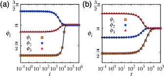
Figure 3: (Color online). Comparison between the time series obtained from the reaction-diffusion models (symbols) and the corresponding phase models (lines). (a) GLE. (b) Ativator-inhibitor model. In this case, three hexagonal cells are aligned in a row, i.e., $\eta_{12}=\eta_{23}=0,d_{12}=d_{23}=\frac{\pi}{3}$.

It should be noted that the phase sensitivity function $\bm{Z}_{0}(\theta)$ is very useful for understanding the response of the polarity orientation to perturbation. See Fig. 2(a) as an example. If the $U$ variable is perturbed upward at $\theta=\pi/2$, $\phi$ will increases because $\bm{Z}_{0}(\pi/2)>0$, i.e., the pattern will eventually shift right.

Analysis–. We focus on the phase model with Eq. (10) below because of the following reason. If $U^{\rm S}(\theta)$ and $Z_{0}^{(U)}(\theta)$ are nearly harmonic, i.e., $u_{k}$ and $z_{k}$ ($k\geq 2$) are small, we approximately obtain $\Gamma_{ij}=-4\pi z_{1}u_{1}[s_{2}^{(ij)}\sin(\phi_{j}-\phi_{i})+s_{2}^{(ij)}\sin 2(\eta_{ij}-\phi_{i})+s_{0}^{(ij)}\sin(2\eta_{ij}-\phi_{i}-\phi_{j})]$, which is Eq. (10) with generally different coefficients. Therefore, the coupling function given by Eq. (10) is of crucial importance.

We first consider two coupled cells with $\eta_{12}=0,\eta_{21}=\pi,a_{12}=a_{21},b_{12}=b_{21}$, and investigate the existence and stability of the in-phase state. Substituting the in-phase state $(\phi_{1},\phi_{2})=(\phi^{*},\phi^{*})$ into Eq. (7) with Eq. (10), we obtain $\sin 2\phi^{*}=0$, thus $\phi^{*}=0,\pi$ or $\phi^{*}=\pm\frac{\pi}{2}$. Putting $\phi_{i}=\phi^{*}+\psi_{i}$ ($i=1,2$), $\xi=\psi_{1}+\psi_{2}$ and $\zeta=\psi_{1}-\psi_{2}$, and linearizing Eq. (7) for small $\psi_{i}$, we obtain

$$\dot{\xi} =-2\epsilon(a_{ij}+b_{ij})(\cos 2\phi^{*})\xi$$ (11)

$$\dot{\zeta} =-2\epsilon a_{ij}(1+\cos 2\phi^{*})\zeta.$$ (12)

The solutions $(0,0)$ and $(\pi,\pi)$ are thus linearly stable when $\epsilon a_{ij}>0$ and $\epsilon(a_{ij}+b_{ij})>0$. The GLE with $\epsilon>0$ satisfies this condition. In contrast, the solution $\phi=\pm\frac{\pi}{2}$ may not be asymptotically stable because $\dot{\zeta}$ always vanishes. The same condition is obtained for the 1D straight chain of any number $N$ of cells with open and periodic boundaries, which can be shown by applying the Gershgorin circle theorem to the corresponding stability matrix.

It should be emphasized that in Eq. (10), the second and third terms contain geometric information in $a_{ij},b_{ij}$ and $\eta_{ij}$ and they facilitate the phase $\phi_{i}$ and the mean phase $\frac{\phi_{i}+\phi_{j}}{2}$ to be oriented to the cell-to-cell direction $\eta_{ij}$, respectively. If only the first term is present in Eq. (10), which is the case in the XY model, there is a family of stable solutions $(\phi_{1},\phi_{2})=(\phi^{*},\phi^{*})$ with arbitrary $\phi^{*}$ values, and the realized polarity pattern is determined by the initial conditions.

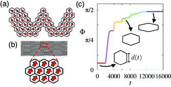
Figure 4: Polarity pattern for (a) winding cell alignment with a regular hexagonal shape and for (b,c) planar alignment of $60\times 20$ cells with elongated shapes obtained numerically with the phase model [Eqs. (7) and (10)]. In (a), the final pattern is displayed with each arrow indicating the phase of each cell. In (b), phases at $t=3000$ are displayed. In (c), the time series of the mean phase $\Phi(t)$ defined as $Q(t)e^{{\rm i}\Phi(t)}=\frac{1}{N}\sum_{j}e^{{\rm i}\phi_{j}(t)}$ with $Q\geq 0$ and $\Phi\in\mathbb{R}$ is displayed. In (b) and (c), cell shape is varied such that the regular hexagon is considered at $t=0$ and $d(t)$ [indicated in (c)] is decreased by $\frac{\pi}{30}$ at $t=2000n$ ($n=1,2,\ldots,7$), while keeping the perimeter $2\pi$. Initial conditions were chosen such that no topological defects appeared.

To obtain useful insight into dynamical behavior for a complicated alignment of cells, we further simplify the phase model using the assumption that the neighboring cells are nearly in phase. Under the approximation that $\phi_{i}=\phi_{j}$ for any neighboring cells, Eq. (7) with Eq. (10) reduces to

$$\dot{\phi}_{i}=\epsilon R_{i}\sin 2(\overline{\eta_{i}}-\phi_{i}),$$ (13)

where $R_{i}>0$ and $\overline{\eta_{i}}\in\mathbb{R}$ are determined by $R_{i}e^{{\rm i}2\overline{\eta_{i}}}=\sum_{j\in A(i)}(a_{ij}+b_{ij})e^{{\rm i}2\eta_{ij}}$, which can be interpreted as the effective strength and the preferred direction of the net interaction of cell $i$, respectively. We first consider square and hexagonal lattices, where the cell has a square and regular hexagonal shape, respectively. In these cases, $R_{i}$ vanishes for cell $i$ not facing boundaries of the lattice because $a_{ij}$ and $b_{ij}$ are not $i,j$-dependent and $\eta_{ij}$ takes the values $0,2\pi/n,4\pi/n,\cdots,2(n-1)\pi/n$ with $n=4$ and $6$ for the square and hexagonal lattices, respectively. On the other hand, for cells at the boundary, $R_{i}$ is non-vanishing and $\overline{\eta_{i}}$ is approximately parallel to the boundary line. Therefore, cell polarity at the boundary is oriented parallel to the boundary line and the bulk is smoothly aligned to that of neighboring cells. As shown in Fig. 4(a), this prediction is confirmed using the system with winding cell alignment. In contrast, when the cell shape is elongated, $R_{i}$ is non-vanishing even in the bulk. In this case, $\overline{\eta_{i}}$ tends to orient to the direction of a contact surface with a larger width. When the number of bulk units is much more than that of boundary units, polarity orientation is dominantly dependent on the cell shape. For example, as shown in Fig. 4(b,c), the polarity tends to be oriented to the direction of the short axis as hexagonal cells are further elongated.

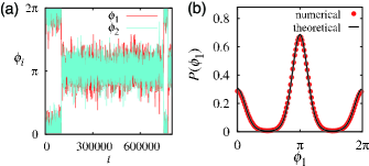
Figure 5: Polarity orientation in the presence of an external signal and noise in the GLE $(N=2)$. (a) Time series obtained numerically from the reaction-diffusion model [Eq. (1)]. (b) The probability density, where $P(\phi_{1})=\int_{0}^{2\pi}P(\phi_{1},\phi_{2})d\phi_{2}$. Numerical results are obtained from direct simulation of Eq. (1) with an inclusion of additive noise $\bm{p}_{i}(\theta_{i},t)=(p_{i}^{(1)},0)$ and external signal $\bm{G}_{i}=(\cos(\psi-\theta_{i}),0)$ with $\psi=\pi$. (a) Time series. (b) The probability density function obtained numerically and the theoretical one $P(\phi_{1})=\int_{0}^{2\pi}P(\phi_{1},\phi_{2})d\phi_{2}$. The parameter values were $\eta_{12}=0,\nu_{1}=0.005$, and $D_{0}=0.2$ (only for this figure).

The phase reduction is also possible when our reaction-diffusion model includes external signal and noise (see Supplemental Material B for details). Specifically, we add to Eq. (1) external signal $\varepsilon_{\rm e}\bm{G}_{i}(\theta_{i},t)$ and white Gaussian noise $\bm{p}_{i}(\theta_{i},t)=(p_{i}^{(1)},p_{i}^{(2)},\ldots)$ that satisfies ${\rm E}[p_{i}^{(m)}]=0$ and ${\rm E}[p_{i}^{(m)}(\theta_{i},t)p_{j}^{(n)}(\theta_{j},t^{\prime})]=\nu_{m}\delta_{ij}\delta_{mn}\delta(\theta_{i}-\theta_{j})\delta(t-t^{\prime})$ where ${\rm E}[\cdot]$ denotes the ensemble average and $\nu_{m}$ is the noise intensity. For sufficiently small $\varepsilon_{\rm e}$ and $\nu_{m}$, we obtain

$$\dot{\phi}_{i}=\varepsilon\sum_{j\in A(i)}\Gamma_{ij}(\phi_{i},\phi_{j})+\varepsilon_{\rm e}\Pi_{i}(\phi_{i})+q_{i},$$ (14)

where $\Pi_{i}(\phi_{i})=\langle\bm{Z}_{0}(\theta_{i}-\phi_{i}),\bm{G}_{i}(\theta_{i})\rangle$ and $q_{i}(t)$ is a white Gaussian noise with zero mean and variance $\nu=\sum_{m}\nu_{m}\int_{0}^{2\pi}{Z^{(m)}(\theta)}^{2}d\theta$ with $Z^{(m)}$ being the $m$th component of $\bm{Z}$. As a simple example, we consider the GLE with $\bm{G}_{i}=(\cos(\psi-\theta_{i}),0)$, where $\psi$ is a parameter, resulting in $\Pi_{i}=\frac{1}{2\sqrt{1-D_{0}}}\sin(\psi-\theta_{i})$. The phase model under consideration is actually a gradient system, i.e., $\dot{\phi}_{i}=-\frac{\partial}{\partial\phi_{i}}\mathcal{H}+q_{i}$ with the potential function $\mathcal{H}=\mathcal{H}(\{\phi_{i}\})$ given in Supplemental Material B for details. We thus obtain probability distribution $P(\{\phi_{i}\})=C\exp\left[-\frac{2\epsilon\mathcal{H}(\{\phi_{i}\})}{\nu}\right]$, where $C$ is the normalization constant. As shown in Fig.  5, the probability distribution obtained numerically from the reaction-diffusion model, Eq. (1), is in excellent agreement with $P(\{\phi_{i}\})$.

Discussion and Conclusion–. A theoretical framework for understanding dynamical properties of alignment process of cellular polarity was proposed. Although the phenomena of our concern are highly nonlinear, our framework enables their analytical treatment even in the presence of noise. Our described framework is readily extendable to treat more concrete problems. For example, the effects of cell heterogeneity and cell shape dependence on local cellular dynamics were examined in previous studies on PCP Amonlirdviman et al. (2005); Aigouy et al. (2010). These factors can be incorporated into our reaction-diffusion model and the resulting phase model and its dynamical behavior would be of great interest. Overall, we expect that our framework would have many potential applications in nonequilibrium systems including chemical and biological systems.

Supplemental Material A Model equations

Our reaction-diffusion model in the absence of perturbation is given as

$$\frac{\partial}{\partial t}\bm{X}_{i} =\bm{F}(\bm{X}_{i})+\hat{D}\frac{\partial^{2}\bm{X}_{i}}{\partial\theta_{i}^{2}}.$$ (S1)

We consider two exmple models: (a)the real Ginzburg-Landau equation (GLE) and (b)the activator-inhibitor model. With $\bm{X}_{i}=(U_{i},V_{i})$, the former reads

$$\bm{F}=\left(\begin{array}[]{c}U_{i}-({U_{i}}^{2}+{V_{i}}^{2})U_{i}\\ V_{i}-({U_{i}}^{2}+{V_{i}}^{2})V_{i})\end{array}\right),$$ (S4)

where $\hat{D}={\rm diag}(D_{0},D_{0})$ and $D_{0}=0.3$. The latter reads

$$\bm{F}=\left(\begin{array}[]{c}\frac{\rho_{U}U_{i}^{2}}{(1+\kappa U_{i}^{2})V_{i}}-\mu_{U}U_{i}+\sigma_{U}\\ \rho_{V}U_{i}^{2}-\mu_{V}V_{i},\end{array}\right),$$ (S7)

where $\rho_{U}=0.01,\rho_{V}=0.02,\mu_{U}=0.01,\mu_{V}=0.02,\sigma_{U}=0.0,\kappa=0.0,\hat{D}={\rm diag}(D_{U},D_{V}),D_{U}=0.005,D_{V}=0.2$, respectively.

Supplemental Material B Phase reduction in the presence of external signal and noise

Our reaction-diffusion model in the presense of intercellular interaction, external signal, and noise is given as

$$\frac{\partial}{\partial t}\bm{X}_{i}=\bm{F}(\bm{X}_{i})+\hat{D}\frac{\partial^{2}}{\partial\theta_{i}^{2}}\bm{X}_{i}+\varepsilon\sum_{j\in A(i)}\bm{H}_{ij}+\varepsilon_{\rm e}\bm{G}_{i}+\bm{p}_{i},$$ (S8)

where $\bm{G}_{i}(\theta_{i},t)$ is the external signal, $\varepsilon_{\rm e}$ is its strength, and $\bm{p}_{i}=(p_{i}^{(1)},p_{i}^{(2)},\ldots)$ is white Gaussian noise that satisfies ${\rm E}[p_{i}^{(m)}(\theta,t)]=0$ and ${\rm E}[p_{i}^{(m)}(\theta,t)p_{j}^{(n)}(\theta^{\prime},t^{\prime})]=\nu_{m}\delta_{ij}\delta_{mn}\delta(\theta-\theta^{\prime})\delta(t-t^{\prime})$, and $\nu_{m}$ is the noise intensity. For sufficiently small $\varepsilon_{\rm e}$ and $\nu_{m}$, we carry on the same procedure as that for Eq. (1) to obtain

$$\dot{\phi}_{i}=\epsilon\sum_{j\in A(i)}\Gamma_{ij}(\phi_{i},\phi_{j})+\varepsilon_{\rm e}\Pi_{i}(\phi_{i},t)+q_{i}(t)$$ (S9)

where

$$\Pi_{i}(\phi_{i}) =\langle\bm{Z}_{0}(\theta_{i}-\phi_{i}),\bm{G}_{i}(\theta_{i},t)\rangle,$$ (S10)

$$q_{i}(t) =\langle\bm{Z}_{0}(\theta_{i}-\phi_{i}),\bm{p}_{i}(\theta_{i},t)\rangle.$$ (S11)

Note that $q_{i}(t)$ is Gaussian white noise that satisfies ${\rm E}[q_{i}(t)]=0$ and ${\rm E}[q_{i}(t)q_{j}(t^{\prime})]=\nu\delta_{ij}\delta(t-t^{\prime})$ with $\nu=\sum_{m}\nu_{m}\int_{0}^{2\pi}d\theta\left\{Z^{(m)}(\theta)\right\}^{2}$ because

$${\rm E}[q_{i}(t)] ={\rm E}\left[\int_{0}^{2\pi}d\theta Z(\theta-\phi_{i})\cdot\bm{p}_{i}(t)d\theta\right]$$ (S12)

$$={\rm E}\left[\int_{0}^{2\pi}d\theta\sum_{m}Z^{(m)}(\theta-\phi_{i})p_{i}^{(m)}d\theta\right]$$ (S13)

$$=\int_{0}^{2\pi}d\theta\sum_{m}Z^{(m)}(\theta-\phi_{i}){\rm E}[p_{i}^{(m)}]d\theta$$ (S14)

$$=0,$$ (S15)

and

$${\rm E}[q_{i}(t)q_{j}(t^{\prime})] ={\rm E}\left[\iint_{0}^{2\pi}d\theta d\theta^{\prime}\{\bm{Z}(\theta-\phi_{i}(t))\cdot\bm{p}_{i}(t)\}\{\bm{Z}(\theta^{\prime}-\phi_{j}(t^{\prime}))\cdot\bm{p}_{j}(t^{\prime})\}\right]$$ (S16)

$$={\rm E}\left[\iint_{0}^{2\pi}\int_{0}^{2\pi}d\theta d\theta^{\prime}\left\{\sum_{m}Z^{(m)}(\theta-\phi_{i}(t))p_{i}^{(m)}(t)\right\}\left\{\sum_{m^{\prime}}Z^{(m^{\prime})}(\theta^{\prime}-\phi_{j}(t^{\prime}))p_{j}^{(m^{\prime})}(t^{\prime})\right\}\right]$$ (S17)

$$={\rm E}\left[\iint_{0}^{2\pi}d\theta d\theta^{\prime}\sum_{m,m^{\prime}}Z^{(m)}(\theta-\phi_{i}(t))p_{i}^{(m)}Z^{(m^{\prime})}(\theta^{\prime}-\phi_{j}(t^{\prime}))p_{j}^{(m^{\prime})}(t^{\prime})\right]$$ (S18)

$$=\iint_{0}^{2\pi}d\theta d\theta^{\prime}\sum_{m,m^{\prime}}Z^{(m)}(\theta-\phi_{i}(t))Z^{(m^{\prime})}(\theta^{\prime}-\phi_{j}(t^{\prime})){\rm E}\left[p_{i}^{(m)}(t)p_{j}^{(m^{\prime})}(t^{\prime})\right]$$ (S19)

$$=\iint_{0}^{2\pi}d\theta d\theta^{\prime}\sum_{m,m^{\prime}}Z^{(m)}(\theta-\phi_{i}(t))Z^{(m^{\prime})}(\theta^{\prime}-\phi_{j}(t^{\prime}))\nu_{m}\delta_{ij}\delta_{mm^{\prime}}\delta(\theta-\theta^{\prime})\delta(t-t^{\prime})$$ (S20)

$$=\int_{0}^{2\pi}d\theta\sum_{m}\nu_{m}\left\{Z^{(m)}(\theta-\phi_{i}(t))\right\}^{2}$$ (S21)

$$=\sum_{m}\nu_{m}\int_{0}^{2\pi}d\theta\left\{Z^{(m)}(\theta)\right\}^{2}.$$ (S22)

In the case of GLE, any generic choice of external signal $\bm{G}_{i}(\theta_{i},t)$ yields

$$\Pi_{i}=c_{i}(t)\sin(\psi_{i}(t)-\theta_{i})$$ (S23)

because $\bm{Z}_{0}(\theta)$ contains only the first harmonics. As a simple example, we consider

$$\bm{G}_{i}(\theta_{i})=(\cos(\psi(t)-\theta_{i}),0),$$ (S24)

where $\psi_{i}(t)$ is a parameter, we obtain

$$\Pi_{i}=\frac{1}{2\sqrt{1-D_{0}}}\sin(\psi-\theta_{i}).$$ (S25)