The Quantum Harmonic Otto Cycle

Abstract

The quantum Otto cycle serves as a bridge between the macroscopic world of heat engines and the quantum regime of thermal devices composed from a single element. We compile recent studies of the quantum Otto cycle with a harmonic oscillator as a working medium. This model has the advantage that it is analytically trackable. In addition, an experimental realization has been achieved, employing a single ion in a harmonic trap. The review is embedded in the field of quantum thermodynamics and quantum open systems. The basic principles of the theory are explained by a specific example illuminating the basic definitions of work and heat. The relation between quantum observables and the state of the system is emphasized. The dynamical description of the cycle is based on a completely positive map formulated as a propagator for each stroke of the engine. Explicit solutions for these propagators are described on a vector space of quantum thermodynamical observables. These solutions which employ different assumptions and techniques are compared. The tradeoff between power and efficiency is the focal point of finite-time-thermodynamics. The dynamical model enables the study of finite time cycles limiting time on the adiabatic and the thermalization times. Explicit finite time solutions are found which are frictionless (meaning that no coherence is generated), and are also known as shortcuts to adiabaticity.The transition from frictionless to sudden adiabats is characterized by a non-hermitian degeneracy in the propagator. In addition, the influence of noise on the control is illustrated. These results are used to close the cycles either as engines or as refrigerators. The properties of the limit cycle are described. Methods to optimize the power by controlling the thermalization time are also introduced. At high temperatures, the Novikov–Curzon–Ahlborn efficiency at maximum power is obtained. The sudden limit of the engine which allows finite power at zero cycle time is shown. The refrigerator cycle is described within the frictionless limit, with emphasis on the cooling rate when the cold bath temperature approaches zero.

I Introduction

Quantum thermodynamics is devoted to the link between thermodynamical processes and their quantum origin. Typically, thermodynamics is applied to large macroscopic entities. Therefore, to what extent is it possible to miniaturize. Can thermodynamics be applicable to the level of a single quantum device? We will address this issue in the tradition of thermodynamics, by learning from an example: Analysis of the performance of a heat engine Carnot (1872). To this end, we review recent progress in the study of the quantum harmonic oscillator as a working medium of a thermal device. The engine composed of a single harmonic oscillator connected to a hot and cold bath is an ideal analytically solvable model for a quantum thermal device. It has therefore been studied extensively and inspired experimental realisation. Recently, a single ion heat engine with an effective harmonic trap frequency has been experimentally realised Roßnagel et al. (2016). This device could roughly be classified as a reciprocating Otto engine operating by periodically modulating the trap frequency.

Real heat engines operate far from reversible conditions. Their performance resides between the point of maximum efficiency and maximum power. This has been the subject of finite time thermodynamics Andresen et al. (1977); Salamon et al. (2001). The topic has been devoted to the irreversible cost of operating at finite power. Quantum engines add a twist to the subject, as they naturally incorporate dynamics into thermodynamics Alicki (1979); Kosloff (1984).

Quantum heat engines can be classified either as continuous or reciprocating. The prototype of a continuous engine is the three-level amplifier pioneered by Scovil and Schulz-DuBois Scovil and Schulz-DuBois (1959). This device is simultaneously coupled to three input currents. It is therefore termed a tricycle, and can operate either as an engine or as a refrigerator. A review of continuous quantum heat engines has been published recently Kosloff and Levy (2014) and therefore is beyond the scope of this review.

Reciprocating engines are classified according to their sequence of strokes. The most studied cycles are Carnot Geva and Kosloff (1992a, b); C. M. Bender, D. c. Brody, B. K. Meister (2002); Lloyd (1997); Esposito et al. (2010) and Otto cycles Feldmann et al. (1996); Quan et al. (2007); He JiZhou, He Xian and Tang Wei (2009); Henrich et al. (2007); Agarwal and Chaturvedi (2013); Zhang et al. (2014). The quantum Otto cycle is easier to analyze, and therefore it became the primary example of a reciprocating quantum heat engine. The pioneering studies of quantum reciprocating engines employed a two-level system—a qubit—as a working medium Geva and Kosloff (1992a, b); Feldmann et al. (1996); J. He, J. Chen and B. Hua (2002). The performance analysis of the quantum versions of reciprocating engines exhibited an amazing resemblance to macroscopic counterparts. For example, the efficiency at maximum power of the quantum version of the endoreversiable engine converges at high temperature to the Novikov–Curzon–Ahlborn macroscopic Newtonian model predictions Novikov (1958); Curzon and Ahlborn (1975). The deviations were even small at low temperature, despite the fact that the heat transport law was different Geva and Kosloff (1992a). The only quantum feature that could be identified was related to the discrete structure of the energy levels.

Heat engines with quantum features require a more complex working medium than a single qubit weakly coupled to a heat bath. This complexity is required to obtain quantum analogues of friction and heat leaks. A prerequisite for such phenomena is that the external control part of the Hamiltonian does not commute with the internal part. This generates quantum non-adiabatic phenomena which lead to friction Kosloff and Feldmann (2002). A working medium composed of a quantum harmonic oscillator has sufficient complexity to represent generic phenomena, but can still be amenable to analytic analysis Rezek and Kosloff (2006).

The quantum Otto cycle is a primary example of the emerging field of quantum thermodynamics. The quest is to establish the similarities and differences in applying thermodynamic reasoning up to the level of a single quantum entity. The present analysis is based on the theory of quantum open systems Kosloff (2013); Gemmer et al. (2009). A dynamical description based on the weak system bath coupling has been able to establish consistency between quantum mechanics and the laws of thermodynamics Kosloff (2013). These links allow work and heat to be defined in the quantum regime Talkner and Hänggi (2016). This framework is sufficient for the present analysis.

In the strong coupling regime where the partition between system and bath is not clear, the connection to thermodynamics is not yet established—although different approaches have been suggested Seifert (2016); Carrega et al. (2016). A different approach to quantum thermodynamics termed quantum thermodynamics resource theory follows ideas from quantum information resource theory, establishing a set of rules  Goold et al. (2016); Vinjanampathy and Anders (2016). We will try to show how this approach can be linked to the Otto cycle under analysis.

II The Quantum Otto Cycle

Nicolaus August Otto invented a reciprocating four stroke engine in 1861, and won a gold medal in the 1867 Paris world fair Otto (1887). The basic components of the engine are hot and cold reservoirs, a working medium, and a mechanical output device. The cycle of the engine is defined by four segments:

1. The hot isochore: heat is transferred from the hot bath to the working medium without volume change.

2. The power adiabat: the working medium expands, producing work, while isolated from the hot and cold reservoirs.

3. The cold isochore: heat is transferred from the working medium to the cold bath without volume change.

4. The compression adiabat: the working medium is compressed, consuming power while isolated from the hot and cold reservoirs, closing the cycle.

Otto determined that the efficiency $\eta$ of the cycle is limited to $\eta_{o}\leq 1-(\frac{V_{h}}{V_{c}})^{\frac{C_{p}}{C_{v}}-1}$, where $V_{c/h}$ and $T_{c/h}$ are the volume and temperature of the working medium at the end of the hot and cold isochores, respectively. $C_{p}$ and $C_{v}$ are the heat capacities under constant pressure and constant volume Callen (2006). As expected, Otto efficiency is always smaller than the efficiency of the Carnot cycle $\eta_{o}\leq\eta_{c}=1-\frac{T_{c}}{T_{h}}$.

The first step in learning from an example is to establish a quantum version of the Otto cycle. This is carried out by seeking analogues for each segment of the cycle. What makes the approach unique is that it is applicable to a small quantum system such as a single atom in a harmonic trap. The description is embedded in the theory of open quantum systems. Each of these segments is defined by a completely positive (CP) propagator Kraus (1971) describing the change of state in the working medium: $\hat{\rho}_{f}={\cal U}_{i\rightarrow f}\hat{\rho}_{i}$, where the density operator $\hat{\rho}$ describes the state of the working medium.

The quantum engine Otto cycle is therefore described as:

1. The hot isochore: heat is transferred from the hot bath to the working medium without change in the external parameter $\omega_{h}$. The stroke is described by the propagator ${\cal U}_{h}$.

2. The expansion adiabat: the working medium reduces its energy scale. The harmonic frequency changes from $\omega_{h}$ to $\omega_{c}$, with $\omega_{h}>\omega_{c}$, producing work while isolated from the hot and cold reservoirs. The stroke is described by the propagator ${\cal U}_{hc}$.

3. The cold isochore: heat is transferred from the working medium to the cold bath without change in the external parameter $\omega_{c}$. The stroke is described by the propagator ${\cal U}_{c}$.

4. The compression adiabat: the working medium increases its energy scale. The harmonic frequencies increase from $\omega_{c}$ to $\omega_{h}$, consuming power while isolated from the hot and cold reservoirs. The stroke is described by the propagator ${\cal U}_{ch}$.

The cycle propagator becomes the product of the segment propagators:

$${\cal U}_{cyc}={\cal U}_{ch}{\cal U}_{c}{\cal U}_{hc}{\cal U}_{h}\;.$$ (1)

The cycle propagator is a completely positive (CP) map of the state of the working medium Kraus (1971). The order of propagators is essential, since the segment propagators do not commute; for example, $[{\cal U}_{h},{\cal U}_{hc}]\neq 0$. The non-commuting property of the segment propagators is not an exclusive quantum property. It is also present in stochastic descriptions of the engine where the propagators operate on a vector of populations of the energy eigenvalues. Nevertheless, it can have a quantum origin for engines with propagators with small action Uzdin et al. (2015, 2016). The same operators but with different parameters (such as different frequencies) can be used to describe an Otto refrigeration cycle. Figure 1 shows a schematic representation of the Otto cycle in phase space.

In the adiabatic limit when the population $N$ stays constant in the expansion and compression segments, the work per cycle becomes:

$${\cal W}_{cyc}=\hbar\Delta\omega\Delta N\;,$$ (2)

where $\Delta\omega=\omega_{h}-\omega_{c}$ and $\Delta N$ is the population difference. $\Delta N=\Delta N_{c}=\Delta N_{h}$, since the cycle is periodic. Under these conditions, the efficiency becomes:

$$\eta_{o}=1-\frac{\omega_{c}}{\omega_{h}}\leq\eta_{c}\;,$$ (3)

where $\eta_{c}$ is the Carnot efficiency $\eta_{c}=1-\frac{T_{c}}{T_{h}}$. At this stage, it is also useful to define the compression ratio ${\cal C}=\frac{\omega_{h}}{\omega_{c}}$.

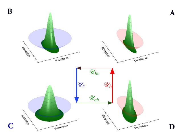
Figure 1: Otto cycle in phase space. The blue and red bowls represent the energy value in position and momentum. The compression ratio is ${\cal C}=\frac{\omega_{h}}{\omega_{c}}=2$. Expansion adiabat $A\rightarrow B$. Cold isochore $B\rightarrow C$. Compression adiabat $C\rightarrow D$. Hot isochore $D\rightarrow A$. The Wigner distribution in phase space is shown in green. The state in $A$ is a thermal equilibrium state with the hot bath temperature. The state in $B$ is squeezed with respect to the cold bath frequency $\omega_{c}$. The state in $C$ is an equilibrium state with the cold bath temperature. The state in $D$ shows position momentum correlation $\langle{\bm{\mathrm{\hat{C}}}}\rangle\neq 0$.

II.1 Quantum Dynamics of the Working Medium

The quantum analogue of the Otto cycle requires a dynamical description of the working medium, the power output, and the heat transport mechanism.

A particle in a harmonic potential will constitute our working medium. This choice is amenable to analytic solutions and has sufficient complexity to serve as a generic example. Even a single specimen is sufficient to realize the operation of an engine.

We can imagine a single particle in a harmonic trap $V(Q)=\frac{k}{2}Q^{2}$. Expansion and compression of the working medium is carried out by externally controlling the trap parameter $k(t)$. The energy of the particle is represented by the Hamiltonian operator:

$${\bm{\mathrm{\hat{H}}}}~{}~{}=~{}~{}\frac{1}{2m}{\bm{\mathrm{\hat{P}}}}^{2}~{}+~{}\frac{k(t)}{2}{{\bm{\mathrm{\hat{Q}}}}^{2}}~{},$$ (4)

where $m$ is the mass of the system and ${\bm{\mathrm{\hat{P}}}}$ and ${\bm{\mathrm{\hat{Q}}}}$ are the momentum and position operators. All thermodynamical quantities will be intensive; i.e., normalized to the number of particles. In the macroscopic Otto engine, the internal energy of the working medium during the adiabatic expansion is inversely proportional to the volume. In the harmonic oscillator, the energy is linear in the frequency $\omega(t)=\sqrt{k(t)/m}$ Boyer (2003). This therefore plays the role of inverse volume $\frac{1}{V}$.

The Hamiltonian (4) is the generator of the evolution on the adiabatic segments. The frequency $\omega$ changes from $\omega_{h}$ to $\omega_{c}$ in a time period $\tau_{hc}$ in the power adiabat ($\omega_{h}>\omega_{c}$) and from $\omega_{c}$ to $\omega_{h}$ in a period $\tau_{ch}$ in the compression adiabat. The dynamics of the state $\hat{\rho}$ during the adiabatic segments is unitary and is the solution of the Liouville von Neumann equation Neumann (1955):

$$\frac{d}{dt}{\hat{\rho}}(t)~{}~{}=~{}~{}-\frac{i}{\hbar}[{\bm{\mathrm{\hat{H}}}}(t),\hat{\rho}(t)]~{},$$ (5)

where ${\bm{\mathrm{\hat{H}}}}$ is time dependent during the evolution. Notice that $[{\bm{\mathrm{\hat{H}}}}(t),{\bm{\mathrm{\hat{H}}}}(t^{\prime})]\neq 0$, since the kinetic energy does not commute with the varying potential energy. This is the origin of quantum friction Kosloff and Feldmann (2002); Plastina et al. (2014). The formal solution to Equation (5) defines the propagator:

$$\hat{\rho}(t)~{}=~{}{\cal U}(t)\hat{\rho}(0)~{}=~{}{\bm{\mathrm{\hat{U}}}}\hat{\rho}(0){\bm{\mathrm{\hat{U}}}}^{\dagger}~{},$$ (6)

where ${\bm{\mathrm{\hat{U}}}}$ satisfies the equation:

$$i\hbar\frac{d}{dt}{\bm{\mathrm{\hat{U}}}}~{}=~{}{\bm{\mathrm{\hat{H}}}}(t){\bm{\mathrm{\hat{U}}}}$$ (7)

with the initial condition ${\bm{\mathrm{\hat{U}}}}(0)={\bm{\mathrm{\hat{I}}}}$.

The dynamics on the hot and cold isochores is a thermalization process of the working medium with a bath at temperature $T_{h}$ or $T_{c}$. The dynamics is of an open quantum system, where the working medium is described explicitly and the bath implicitly Lindblad (1976); Gorini et al. (1976); Breuer and Petruccione (2002):

$$\frac{d}{dt}{\hat{\rho}}(t)~{}~{}=~{}~{}-\frac{i}{\hbar}[{\bm{\mathrm{\hat{H}}}},\hat{\rho}]+{\cal L}_{D}(\hat{\rho})~{},$$ (8)

where ${\cal L}_{D}$ is the dissipative term responsible for driving the working medium to thermal equilibrium, while the Hamiltonian ${\bm{\mathrm{\hat{H}}}}={\bm{\mathrm{\hat{H}}}}(\omega_{h/c})$ is static. The equilibration is not complete in typical operating conditions, since only a finite time $\tau_{h}$ or $\tau_{c}$ is allocated to the hot or cold isochores. The dissipative “superoperator” ${\cal L}_{D}$ must conform to Lindblad’s form for a Markovian evolution Lindblad (1976); Gorini et al. (1976), and for the harmonic oscillator can be expressed as R.S.Ingarden and Kossakowski (1975); Louisell and Louisell (1973); Lindblad (1976):

$$\mathcal{L}_{D}(\hat{\rho})~{}~{}=~{}~{}k_{\uparrow}({\bm{\mathrm{\hat{a}}}}^{\dagger}\hat{\rho}{\bm{\mathrm{\hat{a}}}}~{}-~{}\frac{1}{2}\{{\bm{\mathrm{\hat{a}}}}{\bm{\mathrm{\hat{a}}}}^{\dagger},\hat{\rho}\})+k_{\downarrow}({\bm{\mathrm{\hat{a}}}}\hat{\rho}{\bm{\mathrm{\hat{a}}}}^{\dagger}-\frac{1}{2}\{{\bm{\mathrm{\hat{a}}}}^{\dagger}{\bm{\mathrm{\hat{a}}}},\hat{\rho}\})\;,$$ (9)

where anticommutator $\{{\bm{\mathrm{\hat{A}}}},{\bm{\mathrm{\hat{B}}}}\}\equiv{\bm{\mathrm{\hat{A}}}}{\bm{\mathrm{\hat{B}}}}+{\bm{\mathrm{\hat{B}}}}{\bm{\mathrm{\hat{A}}}}$. $k_{\uparrow}$ and $k_{\downarrow}$ are heat conductance rates obeying detailed balance $\frac{k_{\uparrow}}{k_{\downarrow}}=e^{-\frac{\hbar\omega}{k_{b}T}}$, and $T$ is either $T_{h}$ or $T_{c}$. The operators ${\bm{\mathrm{\hat{a}}}}^{\dagger}$ and ${\bm{\mathrm{\hat{a}}}}$ are the raising and lowering operators, respectively. Notice that they are different in the hot and cold isochores, since ${\bm{\mathrm{\hat{a}}}}=\frac{1}{\sqrt{2}}(\sqrt{\frac{m\omega}{\hbar}}{\bm{\mathrm{\hat{Q}}}}+i\sqrt{\frac{1}{\hbar m\omega}}{\bm{\mathrm{\hat{P}}}})$ depends on $\omega$. Formally for the isochore ${\cal U}_{h/c}=\exp({\cal L}t)$ where ${\cal L}=-i/\hbar[{\bm{\mathrm{\hat{H}}}},\cdot]+{\cal L}_{D}$.

Equation (9) is known as a quantum Master equation Breuer and Petruccione (2002) or L-GKS Lindblad (1976); Gorini et al. (1976). It is an example of a reduced description where the dynamics of the working medium is sought explicitly while the baths are described implicitly by two parameters: the heat conductivity $\Gamma=k_{\downarrow}-k_{\uparrow}$ and the bath temperature $T$. The Lindblad form of Equation (9) guarantees that the density operator of the extended system (system + bath) remains positive (i.e., physical) Lindblad (1976). Specifically, for the harmonic oscillator, Equation (9) has been derived from first principles by many authors Braun and Godoy (1977); Um et al. (2002); Louisell and Louisell (1973); Gardiner and Zoller (2004); Carmichael (2009).

To summarize, the quantum model of the Otto cycle is composed of a working fluid of harmonic oscillators (4). The power stroke is modeled by the Liouville von Neumann equation (5), while the heat transport via a Master equation (8) and (9).

III Quantum Thermodynamics

Thermodynamics is notorious for its ability to describe a process employing an extremely small number of variables. In scenarios where systems are far from thermal equilibrium, further variables have to be added. The analogue description in quantum thermodynamics is based on a minimal set of quantum expectations $\langle{\bm{\mathrm{\hat{X}}}}_{n}\rangle$, where $\langle{\bm{\mathrm{\hat{X}}}}_{n}\rangle=Tr\{{\bm{\mathrm{\hat{X}}}}_{n}\hat{\rho}\}$. The dynamics of this set is generated by the Heisenberg equations of motion

$$\frac{d}{dt}{{\bm{\mathrm{\hat{X}}}}}~{}~{}=~{}~{}\frac{\partial{\bm{\mathrm{\hat{X}}}}}{\partial t}~{}+~{}\frac{i}{\hbar}[{\bm{\mathrm{\hat{H}}}},{\bm{\mathrm{\hat{X}}}}]+{\cal L}^{*}_{D}({\bm{\mathrm{\hat{X}}}})~{},$$ (10)

where the first term addresses an explicitly time-dependent set of operators, ${\bm{\mathrm{\hat{X}}}}(t)$.

The dynamical approach to quantum thermodynamics Kosloff (2013) seeks the relation between thermodynamical laws and their quantum origin.

The first law of thermodynamics is equivalent to the energy balance relation. The energy expectation $E$ is obtained when ${\bm{\mathrm{\hat{X}}}}={\bm{\mathrm{\hat{H}}}}$; i.e., $E=\langle{\bm{\mathrm{\hat{H}}}}\rangle$. The quantum energy partition defining the first law of thermodynamics, $dE=d{\cal W}+d{\cal Q}$, is obtained by inserting ${\bm{\mathrm{\hat{H}}}}$ into (10) Spohn and Lebowitz (2007); Alicki (1979); Kosloff (1984, 2013):

$$\frac{d}{dt}{E}~{}~{}=~{}~{}\dot{\cal W}~{}+~{}\dot{\cal Q}~{}~{}=~{}~{}\langle~{}\frac{\partial{\bm{\mathrm{\hat{H}}}}}{\partial t}~{}\rangle~{}~{}+~{}~{}\langle~{}{\cal L}^{*}_{D}({\bm{\mathrm{\hat{H}}}})~{}\rangle.$$ (11)

The power is identified as

$${\cal P}~{}=~{}\dot{\cal W}~{}=~{}\langle~{}\frac{\partial{\bm{\mathrm{\hat{H}}}}}{\partial t}~{}\rangle.$$

The heat exchange rate becomes

$$\frac{d}{dt}{\cal Q}=\langle~{}{\cal L}^{*}_{D}({\bm{\mathrm{\hat{H}}}})~{}\rangle.$$

The analysis of the Otto cycle benefits from the simplification that power is produced or consumed only on the adiabats and heat transfer takes place only on the isochores.

The thermodynamic state of a system is fully determined by the thermodynamical variables. Statistical thermodynamics adds the prescription that the state is determined by the maximum entropy condition subject to the constraints set by the thermodynamical observables Jaynes (1957a, b); Katz (1967). Maximizing the von Neumann entropy Neumann (1955)

$$S_{VN}=-k_{B}Tr\{\hat{\rho}\ln(\hat{\rho})\}$$ (12)

subject to the energy constraint leads to thermal equilibrium Katz (1967)

$$\hat{\rho}_{eq}~{}~{}=~{}~{}\frac{1}{Z}e^{-\frac{{\bm{\mathrm{\hat{H}}}}}{k_{B}T}}~{},$$ (13)

where $k_{B}$ is the Boltzmann constant and $Z=Tr\{e^{-\frac{{\bm{\mathrm{\hat{H}}}}}{k_{B}T}}\}$ is the partition function.

In general, the state of the working medium is not in thermal equilibrium. In order to generalize the canonical form (13), additional observables are required to define the state of the system. The maximum entropy state subject to this set of observables Alhassid and Levine (1978); jaynes1957a $\langle{\bm{\mathrm{\hat{X}}}}_{j}\rangle=tr\{{{\bm{\mathrm{\hat{X}}}}_{j}}\hat{\rho}\}$ becomes

$$\hat{\rho}~{}~{}=~{}~{}\frac{1}{Z}\exp\left(\sum_{j}~{}\beta_{j}{\bm{\mathrm{\hat{X}}}}_{j}\right),$$ (14)

where $\beta_{j}$ are Lagrange multipliers. The generalized canonical form of (14) is meaningful only if the state can be cast in the canonical form during the entire cycle of the engine, leading to $\beta_{j}=\beta_{j}(t)$. This requirement is called canonical invariance H. C. Andersen I. Opeenheim, K. E. Shuler and H. H. Weiss (1964). It implies that if an initial state belongs to the canonical class of states, it will remain in this class throughout the cycle.

A necessary condition for canonical invariance is that the set of operators ${\bm{\mathrm{\hat{X}}}}$ in (14) is closed under the dynamics generated by the equation of motion. If this condition is satisfied, then the state of the system can be reconstructed from a small number of quantum observables $\langle{\bm{\mathrm{\hat{X}}}}_{j}\rangle(t)$. These become the thermodynamical observables, since they define the state under the maximum entropy principle.

The condition for canonical invariance on the unitary part of the evolution taking place on the adiabats is as follows: if the Hamiltonian is a linear combination of the operators in the set ${\bm{\mathrm{\hat{H}}}}(t)=\sum_{m}h_{m}{\bm{\mathrm{\hat{X}}}}_{m}~{}$ ($h_{m}(t)$ are expansion coefficients), and the set forms a closed Lie algebra $[{\bm{\mathrm{\hat{X}}}}_{j},{\bm{\mathrm{\hat{X}}}}_{k}]=\sum_{l}C^{jk}_{l}{\bm{\mathrm{\hat{X}}}}_{l}$ (where $C^{jk}_{l}$ is the structure factor of the Lie algebra), then the set ${\bm{\mathrm{\hat{X}}}}$ is closed under the evolution Wei and Norman (1963).

For a closed Lie algebra, the generalized Gibbs state Equation (14) can always be written in a product form:

$$\hat{\rho}~{}~{}=~{}~{}\prod_{k}e^{\lambda_{k}{\bm{\mathrm{\hat{X}}}}_{k}}~{},$$ (15)

where there is a one-to-one relation between $\lambda$ and $\beta$, depending on the order of the product form. Multiplying the equation of motion by $\hat{\rho}^{-1}$ leads to $\frac{d}{dt}\hat{\rho}\hat{\rho}^{-1}={\cal L}(\hat{\rho})\hat{\rho}^{-1}$. Using the product form and the Backer–Housdorff relation, the l.h.s. $\frac{d}{dt}\hat{\rho}\hat{\rho}^{-1}$ decomposes to a linear combination of the operator algebra. This is also true for the r.h.s $[{\bm{\mathrm{\hat{H}}}},\hat{\rho}]\hat{\rho}^{-1}$, which also becomes a linear combination of the operator algebra. Comparing both sides of the equation of motion, one obtains a set of coupled differential equations for the coefficients $\lambda_{k}$. Their solution guarantees that canonical invariance prevails Alhassid and Levine (1978).

For the harmonic Otto cycle, the set of the operators ${\bm{\mathrm{\hat{P}}}}^{2}$, ${\bm{\mathrm{\hat{Q}}}}^{2}$, and ${\bm{\mathrm{\hat{D}}}}=\frac{1}{2}({\bm{\mathrm{\hat{Q}}}}{\bm{\mathrm{\hat{P}}}}+{\bm{\mathrm{\hat{P}}}}{\bm{\mathrm{\hat{Q}}}})$ form a closed Lie algebra. Since the Hamiltonian is a linear combination of the first two operators of the set (${\bm{\mathrm{\hat{P}}}}^{2}$ and ${\bm{\mathrm{\hat{Q}}}}^{2}$), canonical invariance will prevail on the adiabatic segments.

On the isochores, the set of operators also has to be closed to the operation of ${\cal L}_{D}$. The set ${\bm{\mathrm{\hat{P}}}}^{2}$, ${\bm{\mathrm{\hat{Q}}}}^{2}$, and ${\bm{\mathrm{\hat{D}}}}$ is closed to ${\cal L}_{D}$, defined by (9). For canonical invariance of $\hat{\rho}$, ${\cal L}_{D}\hat{\rho}\hat{\rho}^{-1}$ should also be a linear combination of operators in the algebra. For the harmonic working medium and ${\cal L}_{D}$ defined in (9), this condition is fulfilled. As a result, canonical invariance with the set of operators ${\bm{\mathrm{\hat{P}}}}^{2}$, ${\bm{\mathrm{\hat{Q}}}}^{2}$, and ${\bm{\mathrm{\hat{D}}}}=\frac{1}{2}({\bm{\mathrm{\hat{Q}}}}{\bm{\mathrm{\hat{P}}}}+{\bm{\mathrm{\hat{P}}}}{\bm{\mathrm{\hat{Q}}}})$ prevails for the whole cycle Rezek and Kosloff (2006).

The significance of canonical invariance is that a solution of the operator dynamics allows the reconstruction of the state of the working medium during the whole cycle. As a result, all dynamical quantities become functions of a very limited set of thermodynamic quantum observables $\langle{\bm{\mathrm{\hat{X}}}}_{j}\rangle$. The choice of a set of operators $\{{\bm{\mathrm{\hat{X}}}}_{j}\}$ should reflect the most essential thermodynamical variables. The operator algebra forms a vector space with the scalar product $\left({\bm{\mathrm{\hat{X}}}}_{j}\cdot{\bm{\mathrm{\hat{X}}}}_{k}\right)=Tr\{{\bm{\mathrm{\hat{X}}}}_{j}^{\dagger}{\bm{\mathrm{\hat{X}}}}_{k}\}$. This vector space will be used to describe the state $\hat{\rho}$ and define the cycle propagators ${\cal U}_{l}$. This description is a significant reduction in the dimension of the propagator ${\cal U}$ from $N^{2}$, where $N$ is the size of Hilbert space to $M$ the size of the operator algebra.

Explicitly, variables with thermodynamical significance are chosen for the harmonic oscillator. These variables are time-dependent and describe the current state of the working medium:

• The Hamiltonian ${\bm{\mathrm{\hat{H}}}}(t)~{}~{}=~{}\frac{1}{2m}{\bm{\mathrm{\hat{P}}}}^{2}+\frac{1}{2}m\omega(t)^{2}{\bm{\mathrm{\hat{Q}}}}^{2}$.

• The Lagrangian ${\bm{\mathrm{\hat{L}}}}(t)=\frac{1}{2m}{\bm{\mathrm{\hat{P}}}}^{2}-\frac{1}{2}m\omega(t)^{2}{\bm{\mathrm{\hat{Q}}}}^{2}$.

• The position momentum correlation $~{}{\bm{\mathrm{\hat{C}}}}(t)=\frac{1}{2}\omega(t)({\bm{\mathrm{\hat{Q}}}}{\bm{\mathrm{\hat{P}}}}+{\bm{\mathrm{\hat{P}}}}{\bm{\mathrm{\hat{Q}}}})=\omega(t){\bm{\mathrm{\hat{D}}}}$.

These operators are linear combinations of the same Lie algebra as ${\bm{\mathrm{\hat{Q}}}}^{2},{\bm{\mathrm{\hat{P}}}}^{2}$, and ${\bm{\mathrm{\hat{D}}}}$. A typical cycle in terms of these variables is shown in Figure 2.

In the algebra of operators, a special place can be attributed to the Casimir operator ${\bm{\mathrm{\hat{G}}}}$. This Casimir commutes with all the operators in the algebra Casimir (1931); Perelomov and Popov (1968). Explicitly, it becomes:

$${\bm{\mathrm{\hat{G}}}}=\frac{{\bm{\mathrm{\hat{H}}}}^{2}-{\bm{\mathrm{\hat{L}}}}^{2}-{\bm{\mathrm{\hat{C}}}}^{2}}{\hbar^{2}\omega^{2}}=\frac{-\left({\bm{\mathrm{\hat{P}}}}{\bm{\mathrm{\hat{Q}}}}+{\bm{\mathrm{\hat{Q}}}}{\bm{\mathrm{\hat{P}}}}\right)^{2}+2{\bm{\mathrm{\hat{P}}}}{\bm{\mathrm{\hat{P}}}}{\bm{\mathrm{\hat{Q}}}}{\bm{\mathrm{\hat{Q}}}}+2{\bm{\mathrm{\hat{Q}}}}{\bm{\mathrm{\hat{Q}}}}{\bm{\mathrm{\hat{P}}}}{\bm{\mathrm{\hat{P}}}}}{4\hbar^{2}}~{}.$$ (16)

Since $[{\bm{\mathrm{\hat{H}}}},{\bm{\mathrm{\hat{G}}}}]=0$, ${\bm{\mathrm{\hat{G}}}}$ is constant under the evolution of the unitary segments generated by ${\bm{\mathrm{\hat{H}}}}$. The Casimir for the harmonic oscillator is a positive operator with a minimum value determined by the uncertainty relation: $\langle{\bm{\mathrm{\hat{G}}}}\rangle\geq\frac{1}{4}$ Boldt et al. (2013).

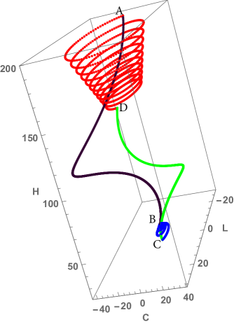
Figure 2: Otto refrigeration cycle displayed in the thermodynamical variables ${\bm{\mathrm{\hat{H}}}},{\bm{\mathrm{\hat{L}}}},{\bm{\mathrm{\hat{C}}}}$. When the working medium is in contact with a hot bath, the system exhausts heat and equilibrates, spiralling downward from a high $\langle{\bm{\mathrm{\hat{H}}}}\rangle$ (energy) value and towards zero correlation $\langle{\bm{\mathrm{\hat{C}}}}\rangle$ and Lagrangian $\langle{\bm{\mathrm{\hat{L}}}}\rangle$ (i.e., towards thermal equilibrium). The hot ishochore is marked by the red dotted line $A\rightarrow D$. On the expansion adiabat, the system spirals downwards, losing energy as it cools down—marked by the green line $D\rightarrow C$. It then spirals upwards (blue line), gaining energy from the cold bath $C\rightarrow B$. In addition , it spirals towards zero $\langle{\bm{\mathrm{\hat{C}}}}\rangle$ and $\langle{\bm{\mathrm{\hat{L}}}}\rangle$. Then, the compression adiabat (black line) takes it back to the top of the hot (red) spiral $B\rightarrow A$.

A related invariant to the dynamics is the Casimir companion Boldt et al. (2013), which for the harmonic oscillator is defined as:

$${\cal X}=\frac{\langle{\bm{\mathrm{\hat{H}}}}\rangle^{2}-\langle{\bm{\mathrm{\hat{L}}}}\rangle^{2}-\langle{\bm{\mathrm{\hat{C}}}}\rangle^{2}}{\hbar^{2}\omega^{2}}~{}.$$ (17)

Combining Equations (16) and (17), an additional invariant to the dynamics can be defined:

$$\frac{1}{\hbar^{2}\omega^{2}}\left(Var({\bm{\mathrm{\hat{H}}}})-Var({\bm{\mathrm{\hat{L}}}})-Var({\bm{\mathrm{\hat{C}}}})\right)=const~{},$$ (18)

where $Var({\bm{\mathrm{\hat{A}}}})=\langle{\bm{\mathrm{\hat{A}}}}^{2}\rangle-\langle{\bm{\mathrm{\hat{A}}}}\rangle^{2}$.

Coherence is an important quantum feature. The coherence is characterised by the deviation of the state of the system from being diagonal in energy Banin et al. (1994); Girolami (2014), and it can be defined as:

$${\cal C}o=\frac{1}{\hbar\omega}\sqrt{\langle{\bm{\mathrm{\hat{L}}}}^{2}\rangle+\langle{\bm{\mathrm{\hat{C}}}}^{2}\rangle}~{}.$$ (19)

From Equation (16), we can deduce that increasing coherence has a cost in energy $\Delta E=\hbar\omega{\cal C}o$.

For the closed algebra of operators, the canonical state of the system $\hat{\rho}$ can be cast into the product form Rezek and Kosloff (2006); Naudts and de Galway (2011). This state $\hat{\rho}$ is defined by the parameters $\beta$, $\gamma$, and $\gamma^{*}$:

$$\hat{\rho}~{}~{}=~{}~{}\frac{1}{Z}e^{\gamma{{\bm{\mathrm{\hat{a}}}}}^{2}}e^{-\beta{{\bm{\mathrm{\hat{H}}}}}}e^{\gamma^{*}{{\bm{\mathrm{\hat{a^{\dagger}}}}}}^{2}}~{},$$ (20)

where ${\bm{\mathrm{\hat{H}}}}=\frac{\hbar\omega}{2}({{\bm{\mathrm{\hat{a}}}}}{{\bm{\mathrm{\hat{a}}}}^{\dagger}}+{{\bm{\mathrm{\hat{a}}}}^{\dagger}}{{\bm{\mathrm{\hat{a}}}}})$, ${\bm{\mathrm{\hat{C}}}}=-i\frac{\hbar\omega}{2}({\bm{\mathrm{\hat{a^{2}}}}}-{\bm{\mathrm{\hat{a^{\dagger}}}}}^{2})$ , ${\bm{\mathrm{\hat{L}}}}=-\frac{\hbar\omega}{2}({\bm{\mathrm{\hat{a}}}}^{2}+{\bm{\mathrm{\hat{a^{\dagger}}}}}^{2})$, and

$$Z~{}~{}=~{}~{}\frac{e^{\frac{\beta\hbar\omega}{2}}}{(e^{\beta\hbar\omega}-1)\sqrt{1-\frac{4\gamma\gamma^{*}}{(e^{\beta\hbar\omega}-1)^{2}}}}~{}.$$ (21)

From (20), the expectations of ${\bm{\mathrm{\hat{H}}}}$ and ${\bm{\mathrm{\hat{a}}}}^{2}$ are extracted, leading to

$$\left\langle{\bm{\mathrm{\hat{H}}}}\right\rangle~{}~{}=~{}~{}\frac{\hbar\omega(e^{2\beta\hbar\omega}-4\gamma\gamma^{*}-1)}{2((e^{\beta\hbar\omega}-1)^{2}-4\gamma\gamma^{*})}~{}~{}and~{}~{}\left\langle{\bm{\mathrm{\hat{a^{2}}}}}\right\rangle~{}~{}=~{}~{}\frac{2\gamma^{*}}{(e^{\beta\hbar\omega}-1)^{2}-4\gamma\gamma^{*}}~{}.$$ (22)

Equation (22) can be inverted, leading to

$$\gamma~{}~{}=~{}~{}\frac{\frac{\hbar\omega}{2}(\left\langle{\bm{\mathrm{\hat{L}}}}\right\rangle+i\left\langle{\bm{\mathrm{\hat{C}}}}\right\rangle)}{\left\langle{\bm{\mathrm{\hat{L}}}}\right\rangle^{2}+\left\langle{\bm{\mathrm{\hat{C}}}}\right\rangle^{2}-(\frac{\hbar\omega}{2}-\left\langle{\bm{\mathrm{\hat{H}}}}\right\rangle)^{2}}$$ (23)

and the inverse temperature $\beta$:

$$e^{\beta\hbar\omega}~{}~{}=~{}~{}\frac{\left\langle{\bm{\mathrm{\hat{L}}}}\right\rangle^{2}+\left\langle{\bm{\mathrm{\hat{C}}}}\right\rangle^{2}-\left\langle{\bm{\mathrm{\hat{H}}}}\right\rangle^{2}+\frac{\hbar^{2}\omega^{2}}{4}}{\left\langle{\bm{\mathrm{\hat{L}}}}\right\rangle^{2}+\left\langle{\bm{\mathrm{\hat{C}}}}\right\rangle^{2}-\left(\frac{\hbar\omega}{2}-\left\langle{\bm{\mathrm{\hat{H}}}}\right\rangle\right)^{2}}~{}~{}.$$ (24)

Equations (23) and (24) relate the state of the system $\hat{\rho}$ (by Equation 20) to the thermodynamical observables $\langle{\bm{\mathrm{\hat{H}}}}\rangle$, $\langle{\bm{\mathrm{\hat{L}}}}\rangle$, and $\langle{\bm{\mathrm{\hat{C}}}}\rangle$.

The generalized canonical state of the system Equation (20) is equivalent to a squeezed thermal state Kim et al. (1989):

$$\hat{\rho}={\bm{\mathrm{\hat{S}}}}({\gamma})\frac{1}{Z}e^{-\beta{\bm{\mathrm{\hat{H}}}}}{\bm{\mathrm{\hat{S}}}}^{\dagger}(\gamma)~{},$$ (25)

with the squeezing operator ${\bm{\mathrm{\hat{S}}}}(\gamma)=\exp(\frac{1}{2}(\gamma^{*}\hat{a}^{2}-\gamma\hat{a}^{\dagger 2}))$. This state is an example of a generalized Gibbs state subject to non-commuting constraints Ilievski et al. (2015); Langen et al. (2015). Figure 1 shows examples of such states, which all have a Gaussian shape in phase space.

Entropy Balance

In thermodynamics, the entropy ${\cal S}$ is a state variable. Shannon introduced entropy as a measure of missing information required to define a probability distribution $\bf p$ Shannon (2001). The information entropy can be applied to a complete quantum measurement of an observable represented by the operator ${\bm{\mathrm{\hat{O}}}}$ with possible outcomes $p_{j}$:

$${\cal S}_{{\bm{\mathrm{\hat{O}}}}}=-k_{B}\sum_{j}~{}p_{j}\ln p_{j}~{},$$ (26)

where $p_{j}=Tr\{{\bm{\mathrm{\hat{P}}}}_{j}\hat{\rho}\}$. The projections ${\bm{\mathrm{\hat{P}}}}_{j}$ are defined using the spectral decomposition theorem ${\bm{\mathrm{\hat{O}}}}=\sum_{j}\lambda_{j}{\bm{\mathrm{\hat{P}}}}_{j}$, where $\lambda_{j}$ are the eigenvalues of the operator ${\bm{\mathrm{\hat{O}}}}$. ${\cal S}_{{\bm{\mathrm{\hat{O}}}}}$ is then the measure of information gain obtained by the measurement.

The von Neumann entropy Neumann (1955) is equivalent to the minimum entropy ${\cal S}_{{\bm{\mathrm{\hat{Y}}}}_{n}}$ associated with a complete measurement of the state $\hat{\rho}$ by the observable ${\bm{\mathrm{\hat{Y}}}}_{n}$, where the set of operators ${\bm{\mathrm{\hat{Y}}}}_{n}$ includes all possible non-degenerate operators in Hilbert space. The operator that minimizes the entropy commutes with the state $[\hat{\rho},{\bm{\mathrm{\hat{Y}}}}_{min}]=0$. This leads to a common set of projectors of ${\bm{\mathrm{\hat{Y}}}}_{min}$ and $\hat{\rho}$; therefore, ${\cal S}_{VN}=-tr\{\hat{\rho}\ln\hat{\rho}\}$, which is a function of the state only. Obviously, ${\cal S}_{VN}\leq{\cal S}_{{\bm{\mathrm{\hat{O}}}}}$. This provides the interpretation that ${\cal S}_{VN}$ is the minimum information required to completely specify the state $\hat{\rho}$.

The primary thermodynamic variable for the heat engine is energy. The entropy associated with the measurement of energy ${\cal S}_{E}={\cal S}_{{\bm{\mathrm{\hat{H}}}}}$ in general differs from the von Neumann entropy ${\cal S}_{E}\geq{\cal S}_{VN}$. Only when $\hat{\rho}$ is diagonal in the energy representation—such as in thermal equilibrium (13)—${\cal S}_{E}={\cal S}_{VN}$.

The relative entropy between the state and its diagonal representation in the energy eigenfucntions is an alternative measure of coherence Baumgratz et al. (2014):

$$D(\hat{\rho}||\hat{\rho}_{ed})=Tr\{\hat{\rho}(\ln\hat{\rho}-\ln\hat{\rho}_{ed})\}~{},$$ (27)

where $\hat{\rho}_{ed}$ is the state composed of the energy projections which has the same populations of the energy levels as state $\hat{\rho}$. The conditional distance $D(\hat{\rho}||\hat{\rho}_{ed})$ is equivalent to the difference between the energy entropy ${\cal S}_{E}$ and the von Neumann entropy ${\cal S}_{VN}$: $D(\hat{\rho}||\hat{\rho}_{ed})={\cal S}_{E}-{\cal S}_{VN}\geq 0$.

The von Neumann entropy is invariant under unitary evolution Alhassid and Levine (1978). This is the result of the property of unitary transformations, where the set of eigenvalues of $\hat{\rho}^{\prime}={\bm{\mathrm{\hat{U}}}}\hat{\rho}{\bm{\mathrm{\hat{U}}}}^{\dagger}$ is equal to the set of eigenvalues of $\hat{\rho}$. Since the von Neumann entropy ${\cal S}_{VN}$ is a functional of the eigenvalues of $\hat{\rho}$, it becomes invariant to any unitary transformation.

When the unitary transformation is generated by members of the Lie algebra, the Casimir is invariant. The von Neumann entropy of the generalized Gibbs state (20) is a function of the Casimir $\langle{\bm{\mathrm{\hat{G}}}}\rangle$ Rezek et al. (2009) so that in this case it also becomes constant:

$${\cal S}_{VN}=\ln\left(\sqrt{\langle{\bm{\mathrm{\hat{G}}}}\rangle-\frac{1}{4}}\right)+\sqrt{\langle{\bm{\mathrm{\hat{G}}}}\rangle}asinh\left(\frac{\sqrt{\langle{\bm{\mathrm{\hat{G}}}}\rangle}}{{\langle{\bm{\mathrm{\hat{G}}}}\rangle-\frac{1}{4}}}\right)~{}.$$ (28)

An alternative expression for the ${\cal S}_{VN}$ entropy is calculated from the covariance matrix of Gaussian canonical states Isar et al. (1999); Serafini et al. (2003); Brown et al. (2016):

$${\cal S}_{VN}=\frac{\nu+1}{2}\ln(\frac{\nu+1}{2})-\frac{\nu-1}{2}\ln(\frac{\nu-1}{2})~{},$$ (29)

where $\nu=\frac{2}{\hbar}\sqrt{\sigma}$,

$$\sigma=\left|\begin{array}[]{cc}\sigma_{pp}&\sigma_{pq}\\ \sigma_{qp}&\sigma_{qq}\end{array}\right|~{},$$ (32)

and $\sigma_{ij}$ is the covariance.

The energy entropy ${\cal S}_{E}$ of the oscillator (not in equilibrium) is found to be equivalent to the entropy of an oscillator in thermal equilibrium with the same energy expectation value:

$${\cal S}_{E}~{}~{}=~{}~{}\frac{1}{\hbar\omega}\left(\left\langle{{\bm{\mathrm{\hat{H}}}}}\right\rangle+\frac{\hbar\omega}{2}\right)\ln\left(\frac{\left\langle\mathbf{\hat{H}}\right\rangle+\frac{\hbar\omega}{2}}{\left\langle\mathbf{\hat{H}}\right\rangle-\frac{\hbar\omega}{2}}\right)-\ln\left(\frac{\hbar\omega}{\left\langle\mathbf{\hat{H}}\right\rangle-\frac{\hbar\omega}{2}}\right)~{}.$$ (33)

${\cal S}_{E}$ in (33) is completely determined by the energy expectation $E=\left\langle\mathbf{{\bm{\mathrm{\hat{H}}}}}\right\rangle$. As an extreme example, for a squeezed pure state, ${\cal S}_{VN}=0$ and ${\cal S}_{E}\geq 0$.

In a macroscopic working medium, the internal temperature can be defined from the entropy and energy variables $1/T_{int}=\left(\frac{\partial{\cal S}}{\partial E}\right)_{V}$ at constant volume. For the quantum Otto cycle, ${\cal S}_{E}$ is used to define the inverse internal temperature $1/T_{int}=\left(\frac{\partial{\cal S}_{E}}{\partial E}\right)_{\omega}$. $T_{int}$ is a generalized temperature appropriate for non equilibrium density operators $\hat{\rho}$. Using this definition, the internal temperature $T_{int}$ of the oscillator working medium can be calculated implicitly from the energy expectation:

$$E=\frac{1}{2}\hbar\omega\coth\left(\frac{\hbar\omega}{2k_{B}T_{int}}\right)~{},$$ (34)

which is identical to the equilibrium relation between temperature and energy in the harmonic oscillator. This temperature defines the work required to generate the coherence: ${\cal W}_{c}=k_{B}T_{int}({\cal S}_{E}-{\cal S}_{VN})$ Plastina et al. (2014).

IV The Dynamics of the Quantum Otto Cycle

A quantum heat engine is a dynamical system subject to the tradeoff between efficiency and power. The dynamics of the reciprocating Otto cycle can be partitioned to the four strokes and later combined to generate the full cycle. Each of the segments influences the final performance: power extraction or refrigeration. The performance of the cycle can be optimized with respect to efficiency and power. Each segment can be optimized separately, and finally a global optimization is performed. The first step is to describe the dynamics of each segment in detail.

IV.1 Heisenberg Dynamics of Thermalisation on the Isochores

The task of the isochores is to extract and reject heat from thermal reservoirs. The dynamics of the working medium is dominated by an approach to thermal equilibrium. In the Otto cycle, the Hamiltonian ${\bm{\mathrm{\hat{H}}}}$ is constant ($\omega=\omega_{h/c}$ is constant). The Heisenberg equations of motion generating the dynamics for an operator ${\bm{\mathrm{\hat{X}}}}$ become:

$$\frac{d}{dt}{{\bm{\mathrm{\hat{X}}}}}=\frac{i}{\hbar}[{\bm{\mathrm{\hat{H}}}},{\bm{\mathrm{\hat{X}}}}]+k_{\downarrow}({\bm{\mathrm{\hat{a}}}}^{\dagger}{\bm{\mathrm{\hat{X}}}}{\bm{\mathrm{\hat{a}}}}-\frac{1}{2}\{{\bm{\mathrm{\hat{a}}}}^{\dagger}{\bm{\mathrm{\hat{a}}}},{\bm{\mathrm{\hat{X}}}}\})+k_{\uparrow}({\bm{\mathrm{\hat{a}}}}{\bm{\mathrm{\hat{X}}}}{\bm{\mathrm{\hat{a}}}}^{\dagger}-\frac{1}{2}\{{\bm{\mathrm{\hat{a}}}}{\bm{\mathrm{\hat{a}}}}^{\dagger},{\bm{\mathrm{\hat{X}}}}\})~{}.$$ (35)

Equation (35) is the analogue of (8) and (9) in the Schrödinger frame.

For the dynamical set of observables, the equations of motion become:

$$\frac{d}{dt}\left(\begin{array}[]{c}{\bm{\mathrm{\hat{H}}}}\\ {\bm{\mathrm{\hat{L}}}}\\ {\bm{\mathrm{\hat{C}}}}\\ {\bm{\mathrm{\hat{I}}}}\end{array}\right)(t)=\left(\begin{array}[]{cccc}-\Gamma&0&0&\Gamma\langle{\bm{\mathrm{\hat{H}}}}\rangle_{eq}\\ 0&-\Gamma&-2\omega&0\\ 0&2\omega&-\Gamma&0\\ 0&0&0&0\end{array}\right)\left(\begin{array}[]{c}{\bm{\mathrm{\hat{H}}}}\\ {\bm{\mathrm{\hat{L}}}}\\ {\bm{\mathrm{\hat{C}}}}\\ {\bm{\mathrm{\hat{I}}}}\end{array}\right)(t)~{},$$ (48)

where $\Gamma=k_{\downarrow}-k_{\uparrow}$ is the heat conductance and $k_{\uparrow}/k_{\downarrow}=e^{-\hbar\omega/k_{B}T}$ obeys detailed balance where $\omega=\omega_{h/c}$ and $T=T_{h/c}$ are defined for the hot or cold bath, respectively. From (11), the heat current can be identified as:

$$\dot{\cal Q}=-\Gamma(\langle{\bm{\mathrm{\hat{H}}}}\rangle-\langle{\bm{\mathrm{\hat{H}}}}\rangle_{eq})~{}~{}=~{}~{}\Gamma\frac{\hbar\omega}{2}\left(\coth(\frac{\hbar\omega}{2k_{B}T_{B}})-\coth(\frac{\hbar\omega}{2k_{B}T_{int}})\right)~{},$$ (49)

where $T_{B}$ is the bath temperature. In the high temperature limit, the heat transport law becomes Newtonian Curzon and Ahlborn (1975): $\dot{\cal Q}=\Gamma(k_{B}T_{B}-K_{B}T_{int})$.

The solution of isochore dynamics (48) generates the propagator defined on the vector space of the observables ${\bm{\mathrm{\hat{H}}}},{\bm{\mathrm{\hat{L}}}},{\bm{\mathrm{\hat{C}}}},{\bm{\mathrm{\hat{I}}}}$: The propagator on the isochore has the form Rezek et al. (2009); Insinga et al. (2016):

$${\cal U}_{h/c}=\left(\begin{array}[]{cccc}R&0&0&H_{eq}(1-R)\\ 0&Rc&-Rs&0\\ 0&Rs&Rc&0\\ 0&0&0&1\end{array}\right)~{},$$ (54)

where $R=e^{-\Gamma t}$. $c=\cos(2\omega t)$, $s=\sin(2\omega t)$, and $H_{eq}=\frac{\hbar\omega}{e^{\frac{\hbar\omega}{kT}}-1}$. It is important to note that the propagator on the isochores does not generate coherence from energy ${\bm{\mathrm{\hat{H}}}}$. The coherence Equation (19) is a function of the expectations of ${\bm{\mathrm{\hat{L}}}},{\bm{\mathrm{\hat{C}}}}$, which are not coupled to ${\bm{\mathrm{\hat{H}}}}$.

IV.2 The Dynamics on the Adiabats and Quantum Friction

The dynamics on the adiabats is generated by a time-dependent Hamiltonian. The task is to change the energy scale of the working medium from one bath to the other. The oscillator frequency changes from $\omega_{h}$ to $\omega_{c}$ on the power expansion segment and from $\omega_{c}$ to $\omega_{h}$ on the compression segment. The Hamiltonian—which is explicitly time-dependent—does not commute with itself at different times $[{\bm{\mathrm{\hat{H}}}}(t),{\bm{\mathrm{\hat{H}}}}(t^{\prime})]\neq 0$. As a result, coherence is generated with an extra cost in energy.

The Heisenberg equations of motion (10) for the dynamical set of operators are expressed as Rezek et al. (2009); Insinga et al. (2016):

$$\frac{d}{dt}\left(\begin{array}[]{c}{\bm{\mathrm{\hat{H}}}}\\ {\bm{\mathrm{\hat{L}}}}\\ {\bm{\mathrm{\hat{C}}}}\\ {\bm{\mathrm{\hat{I}}}}\end{array}\right)(t)=\omega(t)\left(\begin{array}[]{cccc}\mu&-\mu&0&0\\ -\mu&\mu&-2&0\\ 0&2&\mu&0\\ 0&0&0&0\end{array}\right)\left(\begin{array}[]{c}{\bm{\mathrm{\hat{H}}}}\\ {\bm{\mathrm{\hat{L}}}}\\ {\bm{\mathrm{\hat{C}}}}\\ {\bm{\mathrm{\hat{I}}}}\end{array}\right)(t)~{},$$ (55)

where $\mu=\frac{\dot{\omega}}{\omega^{2}}$ is a dimensionless adiabatic parameter. In general, all operators in (55) are dynamically coupled. This coupling is characterized by the non-adiabatic parameter $\mu$. When $\mu\rightarrow 0$, the energy decouples from the coherence and the cycle can be characterized by $p_{n}$—the probability of occupation of energy level $\epsilon_{n}$.

Power is obtained from the first-law (11) as:

$${\cal P}=\mu\omega\left(\langle{\bm{\mathrm{\hat{H}}}}\rangle-\langle{\bm{\mathrm{\hat{L}}}}\rangle\right)~{}.$$ (56)

Power on the adiabats (56) can be decomposed to the “useful” external power ${\cal P}_{ex}=\mu\omega\langle{\bm{\mathrm{\hat{H}}}}\rangle$ and to the power invested to counter friction ${\cal P}_{f}=-\mu\omega\langle{\bm{\mathrm{\hat{L}}}}\rangle$ if $\langle{\bm{\mathrm{\hat{L}}}}\rangle>0$. Under adiabatic conditions $\mu\rightarrow 0$, $\langle{\bm{\mathrm{\hat{L}}}}\rangle=0$, since no coherence is generated; therefore, ${\cal P}_{f}=0$. Generating coherence consumes power when the initial state is diagonal in energy $[\hat{\rho},{\bm{\mathrm{\hat{H}}}}]=0$ Zagoskin et al. (2012); Brandner et al. (2017).

Insight on the adiabatic dynamics can be obtained from the closed-form solution of the dynamics when the non-adiabatic parameter $\mu=\frac{\dot{\omega}}{\omega^{2}}$ is constant. This leads to the explicit time dependence of the control frequency $\omega$: $\omega(t)=\frac{\omega(0)}{1-\mu\omega(0)t}$. Under these conditions, the matrix in Equation (55) becomes stationary. This allows a closed-form solution to be obtained by diagonalizing the matrix. Under these conditions, the adiabatic propagator ${\cal U}_{a}$ has the form:

$${\cal U}_{a}=\frac{\omega(t)}{\omega(0)}\frac{1}{\Omega^{2}}\left(\begin{array}[]{cccc}4-\mu^{2}c&-\mu\Omega s&-2\mu(c-1)&0\\ -\mu\Omega s&\Omega^{2}c&-2\Omega s&0\\ 2\mu(c-1)&2\Omega s&4c-\mu^{2}&0\\ 0&0&0&1\end{array}\right)~{},$$ (61)

where $\Omega=\sqrt{4-\mu^{2}}$ and $c=\cos(\Omega\theta(t))$, $s=\sin(\Omega\theta(t))$, and $\theta(t)=-\frac{1}{\mu}\log(\frac{\omega(t)}{\omega(0)})$ Rezek et al. (2009). For $|\mu|<2$, the solutions are oscillatory. For $|\mu|>2$, the $\sin$ and $\cos$ functions become $\sinh$ and $\cosh$. More on the transition point from damped to over-damped dynamics is presented in Section IV.5.

The difference between the expansion adiabats ${\cal U}_{hc}$ and compression adiabats ${\cal U}_{hc}$ is in the sign of $\mu$ and the ratio $\omega(t)/\omega(0)$. The propagator ${\cal U}_{a}$ can be viewed as a product of a changing energy scale by the factor $\frac{\omega(t)}{\omega(0)}$ and a propagation in a moving frame generated by a constant matrix. The fraction of additional work on the adiabats with respect to the adiabatic solution is causing extra energy invested in the woking medium, which is defined as:

$$\delta_{f}=\frac{\omega_{i}}{\omega_{f}}({\cal U}_{a}(1,1)-\frac{\omega_{f}}{\omega_{i}})~{}.$$ (62)

For the case of $\mu$ constant:

$$\delta_{f}=\frac{2\mu^{2}\sin(\frac{\theta\Omega}{2})^{2}}{4-\mu^{2}}$$ (63)

and $\delta_{f}\geq 0$.

A different approach to the deviation from adiabatic behaviour has been based on a general propagator for Gaussian wavefunctions of the form Deffner et al. (2010):

$$\psi(x,t)=\exp\left(\frac{i}{2\hbar}(a(t)x^{2}+b(t)x+c(t))\right)~{}.$$ (64)

$a(t)$ can be mapped to a time-dependent classical harmonic oscillator: $a(t)=M\dot{X}/X$, where:

$$m\frac{d^{2}}{dt^{2}}X+\omega(t)^{2}X=0~{}.$$ (65)

The local adiabatic parameter is defined as:

$$Q^{*}(t)=\frac{1}{2\omega_{i}\omega_{f}}\left(\omega_{i}^{2}(\omega_{f}^{2}X(t)^{2}+\dot{X}(t)^{2})+(\omega_{f}^{2}Y(t)^{2}+\dot{Y}(t)^{2})\right)~{},$$ (66)

where $X(t)$ and $Y(t)$ are the solution of Equation (65) with the boundary conditions $X(0)=0$, $\dot{X}(0)=1$ and $Y(0)=1$, $\dot{Y}(0)=0$ for a constant frequency $Q^{*}=1$. In general, the expectation value of the energy at the end of the adiabats becomes:

$$\langle{\bm{\mathrm{\hat{H}}}}\rangle_{f}=\frac{\omega_{f}}{\omega_{i}}Q^{*}\langle{\bm{\mathrm{\hat{H}}}}\rangle_{i}~{},$$ (67)

where $i/f$ correspond to the beginning and end of the stroke. In general, $Q^{*}(t)$ can be obtained directly from the solution of Equation (65). $Q^{*}(t)$ is related to $\delta_{f}$ by: $Q^{*}(t)=1+\delta_{f}$. For the case of $\mu$, constant $Q^{*}(t)$ can be obtained from Equation (63). In addition, $Q^{*}(t)$ can be obtained by the solution of the Ermakov equation (Equation (72)) Beau et al. (2016).

The general dynamics described in Equation (61) mixes energy and coherence. As can be inferred from the Casimir Equation (16), generating coherence costs energy. This extra cost gets dissipated on the isochores, and is termed quantum friction Feldmann and Kosloff (2003); Plastina et al. (2014). The energy cost scales as $\mu^{2}$; therefore, slow operation (i.e., $|\mu|\ll 1$) will eliminate this cost. The drawback is large cycle times and low power. Further analysis of Equation (61) shows a surprising result. Coherence can be generated and consumed, resulting in periodic solutions in which the propagator becomes diagonal. As a result, mixing between energy and coherence is eliminated. These solutions appear when $\cos(\Omega\theta(\tau_{a}))=1$, where $\tau_{a}$ is the expansion or compression stroke time allocation. These periodic solutions can be characterised by a quantization relation Rezek et al. (2009):

$$\mu^{*}=-\frac{2\log({\cal C})}{\sqrt{4\pi^{2}l^{2}+\log({\cal C})^{2}}}~{},$$ (68)

where ${\cal C}=\frac{\omega_{c}}{\omega_{h}}$ is the engine’s compression ratio, and $l$ the quantization number $l=1,2,3,...$, accompanied by the time allocation $\tau_{hc}^{*}$:

$$\tau_{hc}^{*}=\frac{1-{\cal C}}{\mu^{*}\omega_{c}}~{}.$$ (69)

A frictionless solution with the shortest time is obtained for $l=1$, and it scales as $\tau_{hc}\propto 1/\omega_{c}$.

This observation raises the question: are there additional frictionless solutions in finite time? What is the shortest time that can achieve this goal?

The general solution of the dynamics depends on an explicit dependence of $\omega(t)$ on time. $\omega(t)$ can be used as a control function to optimise the performance, obtaining a state $\hat{\rho}$ diagonal in energy at the interface with the isochores. Such a solution will generate a frictionless performance. Operating at effective adiabatic conditions has been termed shortcut to adiabaticity Chen et al. (2010); Torrontegui et al. (2013); Chen and Muga (2010); Muga et al. (2010); Cui et al. (2016).

The search for frictionless solutions has led to two main directions. The first is based on a time-dependent invariant operator ${\bm{\mathrm{\hat{I}}}}(t)$ Cui et al. (2016):

$$\frac{d}{dt}{\bm{\mathrm{\hat{I}}}}(t)=\frac{\partial}{\partial t}I(t)+\frac{i}{\hbar}[{\bm{\mathrm{\hat{H}}}}(t),{\bm{\mathrm{\hat{I}}}}(t)]=0~{}.$$ (70)

For the harmonic oscillator, the invariant is Chen et al. (2010):

$${\bm{\mathrm{\hat{I}}}}(t)=\frac{1}{2}\left(\frac{1}{b^{2}}{\bm{\mathrm{\hat{Q}}}}^{2}m\omega_{0}^{2}+\frac{1}{m}{\bm{\mathrm{\hat{\pi}}}}^{2}\right)~{},$$ (71)

where ${\bm{\mathrm{\hat{\pi}}}}=b{\bm{\mathrm{\hat{P}}}}-m\dot{b}{\bm{\mathrm{\hat{Q}}}}$. The invariant must satisfy $[{\bm{\mathrm{\hat{H}}}},{\bm{\mathrm{\hat{I}}}}]=0$ for the initial $\tau_{i}$ and final $\tau_{f}$ times, then at these times the eigenstates of the invariant at the initial and final time of the adiabat are identical to those of the Hamiltonian Torrontegui et al. (2011); Chen et al. (2011). This is obtained if $b(0)=1$ and $\dot{b}(0)=0$, $\ddot{b}(0)=0$, as well as $b(\tau_{f})=\sqrt{\omega_{0}/\omega_{f}}$ and $\dot{b}(\tau_{f})=0$, $\ddot{b}(\tau_{f})=0$. In addition, the function $b(t)$ satisfies the Ermakov equation:

$$\ddot{b}+\omega(t)^{2}b=\omega_{0}^{2}/b^{3}~{}.$$ (72)

The instantaneous frequency becomes $\omega(t)=\omega_{0}/b^{2}$ for $\ddot{b}(0)=0$. There are many solutions to the Ermakov equation, and additional constraints must be added—for example, that the frequency is at all times real and positive. These equations can be used to search for fast frictionless solutions. To obtain a minimal time $\tau_{a}$, some constrains have to be imposed. For example, limiting the average energy stored in the oscillator. In this case, $\tau_{hc}$ scales as $\tau_{hc}^{*}\propto 1/\sqrt{\omega_{c}}$ Chen and Muga (2010). Other constraints on $\omega(t)$ have been explored. For example, the use of imaginary frequency corresponding to an inverted harmonic potential. These schemes allow faster times on the adiabat Chen and Muga (2010); Hoffmann et al. (2011). If the peak energy is constrained, $\tau_{hc}$ scales logarithmically with $1/\omega_{c}$; however, if the average energy is constrained, then the scaling becomes $\tau_{hc}^{*}\propto 1/\sqrt{\omega_{c}}$.

The second approach to obtain frictionless solutions is based on optimal control theory: finding the fastest frictionless solution where the control function is $\omega(t)$ Rezek et al. (2009); Salamon et al. (2009); Hoffmann et al. (2011); Salamon et al. (2012); Hoffmann et al. (2013); Boldt et al. (2016a); Bathaee and Bahrampour (2016). Optimal control theory reveals that the problem of minimizing time is linear in the control, which is proportional to $\omega(t)$ Rezek et al. (2009). As a result, the optimal control solution depends on the constraints $\omega_{max}$ and $\omega_{min}$. If these are set as $\omega_{max}=\omega_{h}$ and $\omega_{min}=\omega_{c}$, then the optimal time scales as $\tau_{a}^{*}\propto\frac{1}{(\sqrt{\omega_{c}}\sqrt{\omega_{c}})}$. Other constraints will lead to faster times, but their energetic cost will diverge. This scaling is consistent considering the cost of the counter-adiabatic terms in frictionless solutions leading to the same scaling Campbell and Deffner (2016).

The optimal solution can be understood using a geometrical description Salamon et al. (2012). The derivative of the change of $\langle{\bm{\mathrm{\hat{Q}}}}^{2}\rangle$ with respect to the change in $\langle{\bm{\mathrm{\hat{P}}}}^{2}\rangle$ becomes:

$$\frac{d\langle{\bm{\mathrm{\hat{Q}}}}^{2}\rangle}{d\langle{\bm{\mathrm{\hat{P}}}}^{2}\rangle}=-\omega^{2}(t)\equiv v~{}.$$ (73)

The time allocated to the change $\tau$ becomes:

$$\tau=\int_{\langle{\bm{\mathrm{\hat{P}}}}^{2}\rangle_{i}}^{\langle{\bm{\mathrm{\hat{P}}}}^{2}\rangle_{f}}\frac{d\langle{\bm{\mathrm{\hat{P}}}}^{2}\rangle}{\sqrt{\langle{\bm{\mathrm{\hat{P}}}}^{2}\rangle\langle{\bm{\mathrm{\hat{Q}}}}^{2}\rangle-\langle{\bm{\mathrm{\hat{G}}}}\rangle}}~{},$$ (74)

where ${\bm{\mathrm{\hat{G}}}}$ is the Casimir defined in Equation (16). In addition, the control $v$ is constrained by $\omega_{c}^{2}\leq v\leq\omega_{h}^{2}$. The initial and final $\langle{\bm{\mathrm{\hat{P}}}}^{2}\rangle_{i/f}=mE_{i/f}$, since the initial and final $\langle{\bm{\mathrm{\hat{L}}}}\rangle$ and $\langle{\bm{\mathrm{\hat{C}}}}\rangle$ are zero. The minimum time is obtained by maximizing the product $\langle{\bm{\mathrm{\hat{P}}}}^{2}\rangle\langle{\bm{\mathrm{\hat{Q}}}}^{2}\rangle$ along the trajectory. The minimum time optimization leads to a bang-bang solution where the frequency is switched instantly from $\omega_{h}$ to $\omega_{c}$, as in the sudden limit Equation (108) is followed by a waiting period then switched back to $\omega_{h}$ until the target is reached and switched finally to $\omega_{c}$. The relation between the geometric optimization and the Ermakov equation of the shortcuts to adiabaticity has been obtained based on the geometrical optimization Stefanatos et al. (2010); Stefanatos (2016).

To summarize, frictionless solutions can be obtained in finite time. As a result, the engine can be completely described by the population of the energy eigenvalues or for the harmonic working medium by the expectation value of number operator ${\bm{\mathrm{\hat{N}}}}$. Employing reasonable constraints on the control function $\omega(t)$ results in the minimum time $\tau_{a}^{*}$ scalling as $O(\frac{1}{\sqrt{\omega_{c}}\sqrt{\omega_{h}}})$.

IV.3 The Influence of Noise on the Adiabats

The frictionless adiabat requires a very accurate protocol of $\omega(t)$ as a function of time. For any realistic devices, such a protocol will be subject to fluctuations in the external control. The controllers are subject to noise, which will induce friction-like behaviour. Can this additional friction be minimized? Insight on the effects of noise on the performance of the Otto cycle can be obtained by analysing a simple model based on the frictionless protocol with constant $\mu$ Torrontegui and Kosloff (2013). The obvious source of external noise is induced by fluctuations in the control frequency $\omega(t)$. This noise is equivalent to Markovian random fluctuations in the frequency of the harmonic oscillator. These errors are modelled by a Gaussian white noise. The dissipative Lindbland term generating such noise has the form Gorini and Kossakowski (1976); Breuer and Petruccione (2002):

$$\mathcal{L}_{N_{a}}(\mathbb{\hat{A}})=-\gamma_{a}\omega^{2}[\mathbb{\hat{B}},[\mathbb{\hat{B}},\mathbb{\hat{A}}]],$$ (75)

where $\mathbb{\hat{B}}=m\omega\mathbb{\hat{Q}}^{2}/(2\hbar)$.

The influence of the amplitude noise generated by $\mathcal{L}_{N_{a}}(\mathbb{\hat{A}})=-\gamma_{a}\omega^{2}[\mathbb{\hat{B}},[\mathbb{\hat{B}},\mathbb{\hat{A}}]]$ is obtained by approximating the propagator by the product form $\mathcal{U}_{hc}=\mathcal{U}_{a}\mathcal{U}_{an}$. The equations of motion for the amplitude noise $\mathcal{U}_{an}$ are obtained from the interaction picture in Liouville space:

$$\frac{d}{\omega dt}\mathcal{U}_{an}(t) = \mathcal{U}_{a}(-t)\mathcal{N}_{a}(t)\mathcal{U}_{a}(t)\mathcal{U}_{an}(t)$$ (76)

$$= \mathcal{W}_{an}(t)\mathcal{U}_{an}(t)~{},$$

where ${\cal W}_{an}$ is the interaction propagator in Liouville space Torrontegui and Kosloff (2013) and ${\cal U}_{a}$ is the adiabatic propagator, Equation (61). A closed-form solution is obtained in the frictionless limit $\mu\rightarrow 0$ when $\mathcal{W}_{a}$ is expanded up to zero order in $\mu$:

$$\mathcal{W}_{a}(t)\approx{\gamma_{a}\omega_{0}}\left(\begin{array}[]{cccc}1&-c&s&0\\ c&-c^{2}&cs&0\\ -s&cs&-s^{2}&0\\ 0&0&0&0\\ \end{array}\right)~{},$$ (81)

where $s=\sin(\Omega\Theta)$ $c=\cos(\Omega\Theta)$. The Magnus expansion Blanes et al. (2009) is employed to obtain the $l$ period propagator $\mathcal{U}_{3a}(X=2l\pi)$, where the periods are of the adiabatic propagator ${\cal U}_{a}$ of Equation (61):

$$\mathcal{U}_{3a}(X=2l\pi)\approx e^{B_{1}+B_{2}+\dotsc}~{},$$ (82)

where $B_{1}=\int_{0}^{2n\pi}dX\mathcal{W}_{a}(X)$, $B_{2}=\frac{1}{2}\int_{0}^{2n\pi}\int_{0}^{X}dXdX^{\prime}[\mathcal{W}_{a}(X),\mathcal{W}_{a}(X^{\prime})]$, and so on. The first-order Magnus term leads to the propagator

$$\mathcal{U}_{an}(X = 2l\pi)_{B_{1}}=\left(\begin{array}[]{cccc}e^{\gamma_{a}{\cal F}/\mu}&0&0&0\\ 0&e^{-\gamma_{a}{\cal F}/(2\mu)}&0&0\\ 0&0&e^{-\gamma_{a}{\cal F}/(2\mu)}&0\\ 0&0&0&1\end{array}\right)~{},$$ (87)

where ${\cal F}=\left(\frac{16\omega_{0}}{(-16+3\mu^{2})}\right)\left(e^{2\pi l\mu\Omega}-1\right)$. For large $l$, in Equation (68) the limit from hot to cold simplifies to: ${\cal F}=(\omega_{h}-\omega_{c})$. The solution of Equation (76) shows that the fraction of work against friction $\delta_{f}$ will diverge when $l\rightarrow\infty$ or $\mu\rightarrow 0$, nulling the adiabatic solution for even a very small $\gamma_{a}$. The best way to eliminate amplitude noise is to choose the shortest frictionless protocol. Nevertheless, some friction-like behaviors will occur.

Next, phase noise is considered. It occurs due to errors in the piecewise process used for controlling the scheduling of $\omega$ in time. For such a procedure, random errors are expected in the duration of the time intervals. These errors are modeled by a Gaussian white noise. Mathematically, the process is equivalent to a dephasing process on the adiabats Feldmann and Kosloff (2006). The dissipative operator $\mathcal{L}_{N}$ has the form given by Gorini and Kossakowski (1976); Breuer and Petruccione (2002):

$$\mathcal{L}_{N_{p}}(\mathbb{\hat{A}})=-\frac{\gamma_{p}}{\hbar^{2}}[\mathbb{\hat{H}},[\mathbb{\hat{H}},\mathbb{\hat{A}}]]~{}.$$ (88)

In this case, the interaction picture for the phase noise ${\cal U}_{p}$ becomes

$$\frac{d}{\omega dt}{\cal U}_{pn}(t) = {\cal U}_{a}(-t){\cal N}_{p}(t){\cal U}_{a}(t)\mathcal{U}_{pn}(t)~{}=~{}{\cal W}_{p}(t){\cal U}_{pn}(t)~{},$$

which at first order in $\mu$ can be approximated as

$${\cal W}_{p}(t)~{}\approx~{}2\gamma_{p}\omega_{0} \times \left(\begin{array}[]{cccc}0&\mu s&\mu(1-c)&0\\ \mu s&-(2+\mu X)&0&0\\ \mu(c-1)&0&-(2+\mu X)&0\\ 0&0&0&0\end{array}\right).$$ (93)

Again, using the Magnus expansion for one period of $X$ leads to

$${\cal U}_{3p}(X=2\pi)_{B_{1}}=\left(\begin{array}[]{cccc}1&0&(1-e^{8\pi\gamma_{p}\omega_{0}})\mu/2&0\\ 0&e^{8\pi\gamma_{p}\omega_{0}}(1-4\pi^{2}\mu\gamma_{p}\omega_{0})&0&0\\ (-1+e^{8\pi\gamma_{p}\omega_{0}})\mu/2&0&e^{8\pi\gamma_{p}\omega_{0}}(1-4\pi^{2}\mu\gamma_{p}\omega_{0})&0\\ 0&0&0&1\end{array}\right)~{}.$$ (98)

At first order in $\mu$, this evolution operator maintains $\delta_{f}(1)=0$, so the frictionless case holds. The second-order Magnus term leads to the noise correction

$${\cal U}_{3p}(X=2\pi)_{B_{2}}=\left(\begin{array}[]{cccc}\cosh\beta&-\sinh\beta&0&0\\ -\sinh\beta&\cosh\beta&0&0\\ 0&0&1&0\\ 0&0&0&1\end{array}\right)~{},$$ (103)

where $\beta=\frac{16\omega_{0}^{2}\gamma_{p}^{2}}{4+3\mu^{2}}\left(e^{2\pi l\mu\Omega}-1\right)$. In the limit of $l\rightarrow\infty$, $\beta=4\gamma^{2}(\omega_{h}^{2}-\omega_{c}^{2})$. The propagator ${\cal U}_{3p}(X=2\pi)_{B_{2}}$ mixes energy and coherence, even at the limit $\mu\rightarrow 0$ and $\tau_{a}\rightarrow\infty$, where one would expect frictionless solutions.

We can characterize the fraction of additional energy generated by a parameter $\delta$. Asymptotically for amplitude noise: $\delta_{a}=e^{\gamma_{a}{\cal F}/\mu}>0$, and for phase noise $\delta_{f}(1)=e^{\gamma_{p}{\cal F}\mu}-1\approx 0$, and the second-order correction $\delta_{f}(2)=\cosh(\beta)-1>0$. Imperfect control on the adiabats will always lead to $\delta_{f}>0$ and additional work invested in friction.

IV.4 The Sudden Limit

The limit of vanishing time on the adiabats $\tau_{a}\ll 1/\omega_{c}$ leads to the sudden propagator; therefore, $\mu\rightarrow\pm\infty$. Such dynamics is termed sudden quench. The propagator ${\cal U}_{a}$ has an explicit expression:

$${\cal U}_{a}=\left(\begin{array}[]{cccc}\frac{1}{2}(1+\alpha)&\frac{1}{2}(1-\alpha)&0&0\\ \frac{1}{2}(1-\alpha)&\frac{1}{2}(1+\alpha)&0&0\\ 0&0&1&0\\ 0&0&0&1\end{array}\right)~{},$$ (108)

where $\alpha=(\frac{\omega_{f}}{\omega_{i}})^{2}$ is related to the compression ratio $\alpha_{ch}={\cal C}^{2}$ and $\alpha_{hc}={\cal C}^{-2}$. The propagator mixes ${\bm{\mathrm{\hat{H}}}}$ and ${\bm{\mathrm{\hat{L}}}}$ when the compression ratio deviates from 1. As a result coherence is generated. The sudden propagator is an integral part of the frictionless bang-bang solutions Rezek et al. (2009); Salamon et al. (2012). Equation (108) can be employed as part of a bang-bang adiabat or as part of a complete sudden cycle.

IV.5 Effects of an Exceptional Point on the Dynamics on the Adiabat

Exceptional points (EPs) are degeneracies of non-Hermitian dynamics Kato (2013); Heiss and Harney (2001) associated with the coalescence of two or more eigenstates. The studies of EPs have substantially grown due to the observation of (space-time reflection symmetry) PT symmetric Hamiltonians Bender (2007). These Hamiltonians have a real spectrum, which becomes complex at the EP. The main effect of EPs (of any order) on the dynamics of PT-symmetric systems is the sudden transition from a real spectrum to a complex energy spectrum Klaiman et al. (2008); Am-Shallem et al. (2015).

The adiabatic strokes are generated by a time-dependent Hamiltonian Equation (4). We therefore expect the propagator ${\cal U}_{a}$ to be unitary, resulting in eigenvalues with the property $|u_{j}|=1$. These properties are only true for a compact Hilbert space. We find surprising exceptions for the non-compact harmonic oscillator with an infinite number of energy levels. We can remove the trivial scaling $\frac{\omega(t)}{\omega(0)}$ in Equation (55) which originates from the diagonal part. The propagator can be written as ${\cal U}_{a}={\cal U}_{0}{\cal U}_{1}$, where ${\cal U}_{0}=\frac{\omega(t)}{\omega(0)}{\cal I}$ is a rescaling of the energy unit. The equation of motion for ${\cal U}_{1}$ becomes:

$$\frac{d}{d\theta}{\cal U}_{1}(\theta)=\left(\begin{array}[]{cccc}0&-\mu&0\\ -\mu&0&-2\\ 0&2&0\\ \end{array}\right){\cal U}_{1}(\theta)~{},$$ (109)

where the trivial propagation of the identity is emitted and the time is rescaled $\theta(t)=\int^{t}\omega(t^{\prime})dt^{\prime}$. Diagonalising Equation (109) for constant $\mu$, we can identify three eigenvalues: $\lambda_{1}=0$ and $\lambda_{23}=\pm i\sqrt{4-\mu^{2}}$. For $\mu\leq 2$, as expected, Equation (109) generates a unitary propagator. The three eigenvalues become degenerate when $\mu=2$, and become real for $\mu\geq 2$ $\lambda_{23}$ Uzdin et al. (2013). This is possible because the generator Equation (109) is non-Hermitian. At the exceptional point, the matrix in Equation (109) has a single eigenvector corresponding to $\lambda_{1}=\lambda_{23}$, which is self-orthogonal. To show this property, it is necessary to multiply the right and left eigenvectors of the non-symmetric matrix at the EP. Their product is equal to zero, showing that the eigenvector is self-orthogonal Moiseyev (2011). The propagator Equation (61) changes character at the EP; $\Omega=\sqrt{4-\mu^{2}}$ changes from a real to an imaginary number. As a result, the dynamics at the EP changes from oscillatory to exponential Uzdin et al. (2013).

This effect can also be observed in the classical parametric oscillator Equation (65). By changing the time variable $\frac{d}{dt}=\omega(t)\frac{d}{d\tau}$, and for constant $\mu$, the equation of motion becomes

$$\left(\frac{d^{2}}{d\tau^{2}}+\mu\frac{d}{d\tau}+1\right)X(\tau)=0~{},$$ (110)

which is the well-known equation of motion of a damped harmonic oscillator. Note that the original model (given by Equation (65)) does not involve dissipation, and a priori one would not expect the appearance of an EP. The rescaling of the time coordinate allows us to identify an EP at $|\mu|=2$, corresponding to the transition between an underdamped and an over-damped oscillator Moiseyev (2013).

Exceptional points are also expected in the eigenvalues and eigenvectors of the total propagator ${\cal U}_{cyc}$, which posses complex eigenvalues. Such points will indicate a drastic change in the cycle performance.

V Closing the Cycle

Periodically combining the four propagators leads to the cycle propagator. Depending on the choice of parameters, we get either an engine cycle where heat flow is converted to power:

$${\cal U}_{cyc}^{e}={\cal U}_{ch}{\cal U}_{c}{\cal U}_{hc}{\cal U}_{h}~{}~{}~{}{\text{where}}~{}~{}\frac{\omega_{c}}{\omega_{h}}>\frac{T_{c}}{T_{h}}~{},$$ (111)

or a refrigerator cycle where power drives a heat current from the cold to the hot bath:

$${\cal U}_{cyc}^{r}={\cal U}_{ch}{\cal U}_{c}{\cal U}_{hc}{\cal U}_{h}~{}~{}~{}{\text{where}}~{}~{}\frac{\omega_{c}}{\omega_{h}}<\frac{T_{c}}{T_{h}}~{}.$$ (112)

In both cases, $\omega_{h}>\omega_{c}$. Frictionless cycles are either refrigerators or engines. Friction adds another possibility. When the internal friction dominates both, the engine cycle and the refrigeration cycle will operate in a dissipative mode, where power is dissipated to both the hot and cold baths. For an engine, this dissipative mode will occur when the internal temperature of the oscillator Equation (34) after the expansion adiabat (cf. Figure 3 point D) will exceed $T_{h}$ and in a refrigerator cycle when the internal temperature exceeds $T_{c}$ (cf. Figure 4 point C).

V.1 Limit Cycle

When a cycle is initiated, after a short transient time it settles to a steady-state operation mode. This periodic state is termed the limit cycle Feldmann and Kosloff (2004); Feldmann et al. (1996). An engine cycle converges to a limit cycle when the internal variables of the working medium reach a periodic steady state. As a result, no energy or entropy is accumulated in the working medium. Figure 2 is an example of a periodic limit cycle. Subsequently, a balance is obtained between the external driving and dissipation. When the cycle time is reduced, friction causes additional heat to be accumulated in the working medium. The cycle adjusts by increasing the temperature gap between the working medium and the baths, leading to increased dissipation. Overdriving leads to a situation where heat is dissipated to both the hot and cold bath and power is only consumed. When this mechanism is not sufficient to stabilise the cycle, one can expect a breakdown of the concept of a limit cycle, resulting in catastrophic consequences Insinga et al. (2016).

The properties of a completely positive (CP) map can be used to prove the existence of a limit cycle. Lindblad Lindblad (1975) has proven that the conditional entropy decreases when applying a trace-preserving completely positive map $\Lambda$ to both the state $\hat{\rho}$ and the reference state $\hat{\rho}_{ref}$:

$$D(\Lambda\hat{\rho}||\Lambda\hat{\rho}_{ref})\leq D(\hat{\rho}||\hat{\rho}_{ref})~{},$$

where $D(\hat{\rho}||\hat{\rho}^{\prime})=Tr(\hat{\rho}(\log\hat{\rho}-\log\hat{\rho}^{\prime}))$ is the conditional entropy distance. A CP map reduces the distinguishability between two states. This can be employed to prove the monotonic approach to steady-state, provided that the reference state $\hat{\rho}_{ref}$ is the only invariant of the CP map $\Lambda$ (i.e., $\Lambda\hat{\rho}_{ref}=\hat{\rho}_{ref}$) Frigerio (1977, 1978); Spohn (1978). This reasoning can prove the monotonic approach to the limit cycle. The mapping imposed by the cycle of operation of a heat engine is a product of the individual evolution steps along the segments composing the cycle propagator. Each one of these evolution steps is a completely positive map, so the total evolution ${\cal U}_{cyc}$ Equation (1) that represents one cycle of operation is also a CP map. If then a state $\hat{\rho}_{lc}$ is found that is a single invariant of ${\cal U}_{cyc}$ (i.e., ${\cal U}_{cyc}\hat{\rho}_{lc}=\hat{\rho}_{lc}$), then any initial state $\hat{\rho}_{init}$ will monotonically approach the limit cycle.

The largest eigenvalue of ${\cal U}_{cyc}$ with a value of $\bf 1$ is associated with the invariant limit cycle state ${\cal U}_{cycr}\hat{\rho}_{lc}=1\hat{\rho}_{lc}$, the fixed point of ${\cal U}_{cyc}$. The other eigenvalues determine the rate of approach to the limit cycle.

In all cases studied of a reciprocating quantum heat engine, a single non-degenerate eigenvalue of $\bf 1$ was the only case found. The theorems on trace preserving completely positive maps are all based on $C^{*}$ algebra, which means that the dynamical algebra of the system is compact. Can the results be generalized to discrete non-compact cases such as the harmonic oscillator? In his study of the Brownian harmonic oscillator, Lindblad conjectured: “in the present case of a harmonic oscillator, the condition that ${\cal L}$ is bounded cannot hold. We will assume this form for the generator with ${\bm{\mathrm{\hat{H}}}}$ and $\cal L$ unbounded as the simplest way to construct an appropriate model” Lindblad (1976). The master equation in Lindblad’s form Equation (9) is well established. Nevertheless, the non-compact character of the resulting map has not been challenged.

A nice demonstration is the study of Insinga et al. Insinga et al. (2016), which shows conditions where a limit cycle is not obtained. This study contains an extensive investigation of the limit cycles as a function of the parameters of the system Insinga et al. (2016).

V.2 Engine Operation and Performance

The engine’s cycle can operate in different modes, which are: adiabatic, frictionless, friction-dominated, and the sudden cycle. In addition, one has to differentiate between two limits: high temperature $k_{B}T\gg\hbar\omega$, where the unit of energy is $k_{B}T$, to low temperature $\hbar\omega\gg k_{B}T$, where the unit of energy is $\hbar\omega$.

In the adiabatic and frictionless cycles Del Campo et al. (2014), the performance can be completely determined by the value of energy at the switching point between strokes.

V.2.1 Optimizing the Work per Cycle

The adiabatic limit with infinite time allocations on all segments maximises the work. No coherence is generated, and therefore the cycle can be described by the change in energy. On the expansion adiabat $E_{B}=\frac{\omega_{c}}{\omega_{h}}E_{A}$, and on the compression adiabat $E_{D}=\frac{\omega_{h}}{\omega_{c}}E_{C}$. As a result, when the cycle is closed, the heat transferred to the hot bath ${\cal Q}_{h}=E^{A}-E^{D}$ and to the cold bath ${\cal Q}_{c}=E_{B}-E_{C}$ are related: $\frac{{\cal Q}_{c}}{{\cal Q}_{h}}=\frac{\omega_{c}}{\omega_{h}}$.

The efficiency for an engine becomes the Otto efficiency:

$$\eta=\frac{\cal W}{{\cal Q}_{h}}=1-\frac{\omega_{c}}{\omega_{h}}\leq 1-\frac{T_{c}}{T_{h}}~{}.$$ (113)

Choosing the compression ratio ${\cal C}=\frac{\omega_{h}}{\omega_{c}}=\frac{T_{h}}{T_{c}}$ maximises the work and leads to Carnot efficiency $\eta_{o}=\eta_{c}$. Since for this limit the cycle time $\tau_{cyc}$ is infinite, the power ${\cal P}={\cal W}/\tau_{cyc}$ of this cycle is obviously zero.

V.2.2 Optimizing the Performance of the Engine for Frictionless Conditions

Frictionless solutions allow finite time cycles with the same efficiency $\eta_{o}=1-\frac{\omega_{c}}{\omega_{h}}$ as the adiabatic case. A different viewpoint is to account as wasted work the average energy invested in achieving the frictionless solution, termed superadiabatic drive Abah and Lutz (2016):

$$\eta=\frac{\cal W}{{\cal Q}_{h}+\langle H_{ch}\rangle+\langle H_{hc}\rangle}~{},$$ (114)

where $\langle H_{ch}\rangle$ is the average additional energy during the adiabatc stroke. Using for example Equation (61), the average additional energy becomes $\langle H_{ch}\rangle=\frac{\omega_{h}}{\omega_{c}}E_{C}\frac{\mu^{2}}{4-\mu^{2}}$, which vanishes as the non-adiabatic parameter $\mu\rightarrow 0$. This additional energy $\langle H_{ch}\rangle$ in the engine is the price for generating coherence. Coherence is exploited to cancel friction. This extra energy is not dissipated, and can therefore be viewed as a catalyst. For this reason, we do not accept the viewpoint of Abah and Lutz (2016).

In our opinion, what should be added to the accounting is the additional energy generated by noise on the controls:

$$\eta=\frac{\cal W}{{\cal Q}_{h}+E_{C}\delta_{ch}+E_{A}\delta_{hc}}\leq\eta_{o}~{},$$ (115)

where $\delta_{hc}=\delta_{a}+\delta_{f}$ for the power adiabat and $\delta_{a}$ and $\delta_{f}$ are generated by amplitude and phase noise on the controller (cf. Section IV.3). A similar relation is found for the compression adiabat.

Optimizing power requires a finite cycle time $\tau_{cyc}$. Optimisation is carried out with respect to the time allocations on each of the engine’s segments: $\tau_{h}$, $\tau_{hc}$, $\tau_{c}$, and $\tau_{ch}$. This sets the total cycle time $\tau_{cyc}=\tau_{h}+\tau_{hc}+\tau_{c}+\tau_{ch}$. The time allocated to the adiabats is constrained by the frictionless solutions $\tau_{hc}^{*}$ and $\tau_{ch}^{*}$. The resulting optimization is very close to the unconstrained optimum Insinga et al. (2016), especially in the interesting limit of low temperatures. The frictionless conditions are obtained either from Equation (68) or from other shortcuts to adiabaticity methods Equation (70). In the frictionless regime, the number operator is fixed at both ends of the adiabat. The main task is therefore to optimize the time allocated to thermalisation on the isochores. This heat transport is the source of entropy production.

The time allocations on the isochores determine the change in the number operator $N=\langle{\bm{\mathrm{\hat{N}}}}\rangle=\frac{1}{\hbar\omega}\langle{\bm{\mathrm{\hat{H}}}}\rangle$ (cf. Equation (48)): $N^{\bf B}=e^{-\Gamma_{h}\tau_{h}}\left(N^{\bf A}-N_{eq}^{h}\right)+N_{eq}^{h}$ on the hot isochore, where $N^{\bf B}$ is the number expectation value at the end of the hot isochore, $N^{\bf A}$ at the beginning, and $N_{eq}^{h}$ is the equilibrium value point E. A similar expression exists for the cold isochore.

Work in the limit cycle becomes

$${\cal W}_{q}~{}~{}=~{}~{}E^{\bf C}-E^{\bf B}+E^{\bf A}-E^{\bf D}~{}~{}=~{}~{}\hbar(\omega_{c}-\omega_{h})(N^{\bf B}-N^{\bf D})~{},$$ (116)

where the convention of the sign of the work for a working engine is negative, in correspondance with Callen Callen (2006), and we use the convention of Figure 3 to mark the population and energy at the corners of the cycle.

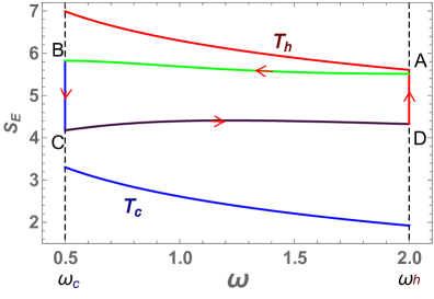
Figure 3: Typical engine cycle ${\cal S}_{E}~{}$ vs. $~{}\omega$. Expansion adiabat $A\rightarrow B$. Cold isochore $B\rightarrow C$. Compression adiabat $C\rightarrow D$. Hot isochore $D\rightarrow A$. The hot and cold isotherms are indicated. The cycle parameters are $\omega_{c}=0.5,~{}T_{c}=5,~{}\omega_{h}=2,~{}T_{h}=200,~{}\tau_{c}=\tau_{h}=2.1,~{}|\mu|=0.8~{}\Gamma=1$.

The heat transport from the hot bath becomes

$${\cal Q}_{h}~{}~{}=~{}~{}E^{\bf B}-E^{\bf D}~{}~{}=~{}~{}\hbar\omega_{h}(N^{\bf B}-N^{\bf D})~{}.$$ (117)

In the limit cycle for frictionless conditions, $N^{\bf B}=N^{\bf A}$, which leads to the relation

$$N^{\bf B}=\frac{(e^{\Gamma_{c}\tau_{c}}-1)}{1-e^{\Gamma_{c}\tau_{c}+\Gamma_{h}\tau_{h}}}(N_{eq}^{h}-N_{eq}^{c})+N_{eq}^{h}~{}.$$ (118)

In the periodic limit cycle, the number operator change $N^{\bf B}-N^{\bf D}$ is equal on the hot and cold isochores, leading to the work per cycle:

$${\cal W}_{q} = \hbar(\omega_{h}-\omega_{c})(N_{eq}^{h}-N_{eq}^{c})\frac{(e^{x_{c}}-1)(e^{x_{h}}-1)}{1-e^{x_{c}+x_{h}}}$$

$$\equiv -G_{W}(T_{c},\omega_{c},T_{h},\omega_{h})F(x_{c},x_{h})~{},$$

where the scaled time allocations are defined $x_{c}\equiv\Gamma_{c}\tau_{c}$ and $x_{h}\equiv\Gamma_{h}\tau_{h}$. The work ${\cal W}_{q}$ Equation (V.2.2) becomes a product of two functions: $G_{W}$, which is a function of the static constraints of the engine, and $F$, which describes the heat transport on the isochores. Explicitly, the function $G_{W}$ is

$$G_{W}(T_{c},\omega_{c},T_{h},\omega_{h})=\frac{\hbar}{2}\left(\omega_{h}-\omega_{c}\right)\left(\coth\left(\frac{\hbar\omega_{h}}{2k_{B}T_{h}}\right)-\coth\left(\frac{\hbar\omega_{c}}{2k_{B}T_{c}}\right)\right)~{}.$$ (120)

The function $F$ in Equation (V.2.2) is bounded $0\leq F\leq 1$; therefore, for the engine to produce work, $G_{W}\geq 0$. The first term in (120) is positive. Therefore, $G_{W}\geq 0$ requires that $\frac{\omega_{c}}{\omega_{h}}\geq\frac{T_{c}}{T_{h}}$, or in terms of the compression ratio, $1\leq{\cal C}\leq\frac{T_{h}}{T_{c}}$. This is equivalent to the statement that the maximum efficiency of the Otto cycle is smaller than the Carnot efficiency $\eta_{o}\leq\eta_{c}$.

In the high temperature limit when $\frac{\hbar\omega}{k_{B}T}\ll 1$, $G_{W}$ simplifies to

$$G_{W}~{}~{}=~{}~{}k_{B}T_{c}(1-{\cal C})~{}+~{}k_{B}T_{h}(1-{\cal C}^{-1})~{}.$$ (121)

In this case, the work ${\cal W}_{q}=-G_{W}~{}F$ can be optimized with respect to the compression ratio ${\cal C}=\frac{\omega_{h}}{\omega_{c}}$ for fixed bath temperatures. The optimum is found at ${\cal C}=\sqrt{\frac{T_{h}}{T_{c}}}$. As a result, the efficiency at maximum power for high temperatures becomes

$$\eta_{q}=1-\sqrt{\frac{T_{c}}{T_{h}}}~{},$$ (122)

which is the well-known efficiency at maximum power of an endo-reversible engine Novikov (1958); Curzon and Ahlborn (1975); Esposito et al. (2009, 2010); Geva and Kosloff (1992a); Kosloff (1984). Note that these results indicate greater validity to the Novikov–Curzon–Ahlbourn result from what their original derivation Curzon and Ahlborn (1975) indicates.

The function $F$ defined in (V.2.2) characterizes the heat transport to the working medium. As expected, $F$ maximizes when infinite time is allocated to the isochores. The optimal partitioning of the time allocation between the hot and cold isochores is obtained when:

$$\Gamma_{h}(\cosh(\Gamma_{c}\tau_{c})-1)=\Gamma_{c}(\cosh(\Gamma_{h}\tau_{h})-1)~{}.$$ (123)

If (and only if) $\Gamma_{h}=\Gamma_{c}$, the optimal time allocations on the isochores becomes $\tau_{h}=\tau_{c}$.

Optimising the total cycle power output ${\cal P}$ is equivalent to optimizing $F/\tau_{cyc}$, since $G_{W}$ is determined by the engine’s external constraints. The total time allocation $\tau_{cyc}=\tau_{iso}+\tau_{adi}$ is partitioned to the time on the adiabats $\tau_{adi}$, which is limited by the adiabatic frictionless condition, and the time $\tau_{iso}$ allocated to the isochores.

Optimising the time allocation on the isochores subject to (123) leads to the optimal condition

$$\Gamma_{c}\tau_{cyc}(\cosh(\Gamma_{h}\tau_{h})-1)=\sinh(\Gamma_{h}\tau_{h}+\Gamma_{c}\tau_{c})-\sinh(\Gamma_{c}\tau_{c})-\sinh(\Gamma_{h}\tau_{h})~{}.$$ (124)

When $\Gamma_{h}=\Gamma_{c}\equiv\Gamma$, this expression simplifies to:

$$2x+\Gamma\tau_{adi}=2\sinh(x)~{},$$ (125)

where $x=\Gamma_{c}\tau_{c}=\Gamma_{h}\tau_{h}$. For small $x$, Equation (125) can be solved, leading to the optimal time allocation on the isochores: $\tau_{c}=\tau_{h}\approx\left(\Gamma\tau_{adi}/3\right)^{\frac{1}{3}}/\Gamma$. Considering the restriction due to frictionless condition Salamon et al. (2009), this time can be estimated to be: $\tau_{c}=\tau_{h}\approx\frac{1}{\Gamma}\left(\frac{\Gamma}{\sqrt{\omega_{c}\omega_{h}}}\right)^{\frac{1}{3}}$. When the heat transport rate $\Gamma$ is sufficiently large, the optimal power conditions lead to the bang-bang solution where vanishingly small time is allocated to all segments of the engine Feldmann et al. (1996) and $\tau_{cyc}\approx 2\tau_{adi}$.

The entropy production $\Delta S_{U}$ reflects the irreversible character of the engine. In frictionless conditions, the irreversibility is completely associated with the heat transport. $\Delta S_{U}$ can also be factorized to a product of two functions:

$$\Delta S_{u}~{}~{}=~{}~{}G_{S}(T_{c},\omega_{c},T_{h},\omega_{h})F(x_{c},x_{h})~{},$$ (126)

where $F$ is identical to the $F$ function defined in (V.2.2). The function $G_{S}$ becomes:

$$G_{S}(T_{c},\omega_{c},T_{h},\omega_{h})~{}~{}=~{}~{}\frac{1}{2}\left(\frac{\hbar\omega_{h}}{k_{B}T_{h}}-\frac{\hbar\omega_{c}}{k_{B}T_{c}}\right)\left(\coth\left(\frac{\hbar\omega_{c}}{2k_{B}T_{c}}\right)-\coth\left(\frac{\hbar\omega_{h}}{2k_{B}T_{h}}\right)\right)~{}.$$ (127)

Due to the common $F(x_{c},x_{h})$ function, the entropy production has the same dependence on the time allocations $\tau_{h}$ and $\tau_{c}$ as the work ${\cal W}$ Feldmann and Kosloff (2000). As a consequence, maximizing the power will also maximize the entropy production rate $\Delta S_{u}/\tau_{cyc}$. Note that entropy production is always positive, even for cycles that produce no work, as their compression ratio $\cal C$ is too large, which is a statement of the second law of thermodynamics.

The dependence of the $G_{s}$ function on the compression ratio can be simplified in the high temperature limit, leading to:

$$G_{S}~{}~{}=~{}~{}{\cal C}\frac{T_{c}}{T_{h}}+{\cal C}^{-1}\frac{T_{h}}{T_{c}}-2~{},$$ (128)

which is a monotonic decreasing function in the range $1\leq{\cal C}\leq\frac{T_{h}}{T_{c}}$ that reaches a minimum at the Carnot boundary when ${\cal C}=\frac{T_{h}}{T_{c}}$. When power is generated, the entropy production rate in the frictionless engine is linearly proportional to the power:

$${\cal S}_{u}=\left(\frac{\hbar\omega_{h}}{k_{B}T_{h}}-\frac{\hbar\omega_{c}}{k_{B}T_{c}}\right)\left(\frac{1}{\omega_{h}-\omega_{c}}\right){\cal P}~{}.$$ (129)

Frictionless harmonic cycles have been studied under the name of superadiabatic driving Del Campo et al. (2014). The frictionless adiabats are obtained using the methods of shortcut to adiabaticity Cui et al. (2016) and the invariant Equation (70). An important extension applies shortcuts to adiabaticity to working mediums composed of interacting particles in a harmonic trap Wang et al. (2015); Jaramillo et al. (2016); Beau et al. (2016); Chotorlishvili et al. (2016).

A variant of the Otto engine is an addition of projective energy measurements before and after each adiabat. This construction is added to measure the work output Zheng et al. (2016). As a result, the working medium is always diagonal in the energy basis. In the frictionless case, the cycle is not altered by this projective measurement of energy.

V.2.3 The Engine in the Sudden Limit

The extreme case of the performance of an engine with zero time allocation on the adiabats is dominated by the frictional terms. These terms arise from the inability of the working medium to adiabatically follow the external change in potential. A closed-form expression for the sudden limit can be derived based on the adiabatic branch propagator ${\cal U}_{hc}$ and ${\cal U}_{ch}$ in Equation (108).

To understand the role of friction, we demand that the heat conductance terms $\Gamma$ are very large, thus eliminating the thermalisation time. In this limiting case, the work per cycle becomes:

$${\cal W}_{s}~{}~{}=~{}~{}\frac{(\omega_{c}-\omega_{h})(\omega_{c}+\omega_{h})}{4\omega_{c}\omega_{h}}\left(\hbar\omega_{c}\coth(\frac{\hbar\omega_{h}}{2k_{B}T_{h}})-\hbar\omega_{h}\coth(\frac{\hbar\omega_{c}}{2k_{B}T_{c}})\right)~{}.$$ (130)

The maximum produced work $-{\cal W}_{s}$ can be optimised with respect to the compression ratio $\cal C$. At the high temperature limit:

$${\cal W}_{s}=\frac{1}{2}k_{B}T_{h}({\cal C}^{2}-1)(\frac{T_{c}}{T_{h}}-\frac{1}{{\cal C}^{2}})~{}.$$ (131)

For the frictionless optimal compression ratio ${\cal C}=\sqrt{\frac{T_{h}}{T_{c}}}$, ${\cal W}_{s}$ is zero. The optimal compression ratio for the sudden limit becomes: ${\cal C}=\left(\frac{T_{h}}{T_{c}}\right)^{1/4}$, leading to the maximal work in the high temperature limit

$${\cal W}_{s}~{}~{}=~{}~{}-\frac{1}{2}k_{B}T_{c}\left(~{}1-\sqrt{\frac{T_{h}}{T_{c}}}~{}\right)^{2}~{}.$$ (132)

The efficiency at the maximal work point becomes:

$$\eta_{s}~{}~{}=~{}~{}\frac{1-\sqrt{\frac{Th}{Tc}}}{2+\sqrt{\frac{Th}{Tc}}}~{}.$$ (133)

Equation (133) leads to the following hierarchy of the engine’s maximum work efficiencies:

$$\eta_{s}~{}\leq~{}\eta_{q}~{}\leq~{}\eta_{c}~{}.$$ (134)

Equation (134) leads to the interpretation that when the engine is constrained by friction its efficiency is smaller than the endo-reversible efficiency, where the engine is constrained by heat transport that is smaller than the ideal Carnot efficiency. At the limit of $T_{c}\rightarrow 0$, we have $\eta_{s}=\frac{1}{2}$ and $\eta_{q}=\eta_{c}=1$ Uzdin and Kosloff (2014).

An upper limit to the work invested in friction ${\cal W}_{f}$ is obtained by subtracting the maximum work in the frictionless limit Equation (V.2.2) from the maximum work in the sudden limit Equation (130). In both these cases, infinite heat conductance is assumed, leading to $N^{B}=N_{eq}^{h}$ and $N^{D}=N_{eq}^{c}$. Then, the upper limit of work invested to counter friction becomes:

$${\cal W}_{f}~{}~{}=~{}~{}\hbar\omega_{h}\frac{({\cal C}-1)^{2}(1+{\cal C}+2{\cal C}N_{eq}^{c}+2N_{eq}^{h})}{4{\cal C}^{2}}~{}.$$ (135)

At high temperature, Equation (135) changes to:

$${\cal W}_{f}~{}~{}=~{}~{}\frac{1}{2}k_{b}T_{h}({\cal C}-1)^{2}({\cal C}^{-2}+\frac{T_{c}}{T_{h}})~{}.$$ (136)

The maximum produced work at the high temperature limit of the frictionless and sudden limits differ by the optimal compression ratio. For the frictionless case, ${\cal C}^{*}=\sqrt{\frac{T_{h}}{T_{c}}}$, and for the sudden case, ${\cal C}^{*}=(\frac{T_{h}}{T_{c}})^{1/4}$.

The work against friction ${\cal W}_{f}$ (Equation (136)) is an increasing function of the temperature ratio. For the compression ratio that optimises the frictionless limit, the sudden work is zero. At this compression ratio, all the useful work is balanced by the work against friction ${\cal W}_{f}={\cal W}_{q}$. Beyond this limit, the engine transforms to a dissipator, generating entropy at both the hot and cold baths. This is in contrast to the frictionless limit, where the compression ratio ${\cal C}=\frac{T_{h}}{T_{c}}$ leads to zero power.

The complete sudden limit assumes short time dynamics on all segments including the isochores. These cycles with vanishing cycle times approach the limit of a continuous engine. The short time on the isochores means that coherence can survive. Friction can be partially avoided by exploiting this coherence, which—unlike the frictionless engine—is present in the four corners of the cycle. The condition for such cycles is that the time allocated is much smaller than the natural period set by the frequency $\tau_{c},\tau_{h}\ll 2\pi/\omega$ and by heat transfer $\tau_{c},\tau_{h}\ll 1/\Gamma$. The heat transport from the hot and cold baths in each stroke becomes very small. For simplicity, $\Gamma_{h}\tau_{h}=\Gamma_{c}\tau_{c}$ is  chosen to be balanced. Under these conditions, the cycle propagator becomes:

$${\cal U}_{cyc}~{}=~{}\left(\begin{array}[]{cccc}(1-g)^{2}&0&0&[g(1-g)\frac{1}{2}(1+{\cal C}^{2})\hbar\omega_{c}N_{c}^{eq}+g\hbar\omega_{h}N_{h}^{eq}]\\ 0&(1-g)^{2}&0&(1-g)g\frac{1}{2}(1-{\cal C}^{2})\hbar\omega_{c}N_{c}^{eq}\\ 0&0&(1-g)^{2}&0\\ 0&0&0&1\end{array}\right)~{},$$ (141)

where the degree of thermalisation is $g=1-R\approx\Gamma_{h}\tau_{h}$. Observing Equation (141), it is clear that the limit cycle vector contains both ${\bm{\mathrm{\hat{H}}}}$ and ${\bm{\mathrm{\hat{L}}}}$.

The work output per cycle becomes:

$${\cal W}_{S}=-\hbar\omega_{h}\frac{g}{2-g}\frac{{\cal C}^{2}-1}{2{\cal C}^{2}}\left(N_{h}^{eq}-{\cal C}N_{c}^{eq}\right)~{}.$$ (142)

Extractable work is obtained in the compression range of $1<{\cal C}<\frac{N_{h}^{eq}}{N_{c}^{eq}}$. The maximum work is obtained when ${\cal C}^{*}=\left(\frac{N_{h}^{eq}}{N_{c}^{eq}}\right)^{1/4}$. At high temperature, the work per cycle simplifies to:

$${\cal W}_{S}\approx-k_{B}T_{c}\frac{\Gamma\tau}{2}\frac{{\cal C}^{2}-1}{2{\cal C}^{2}}\left(\frac{T_{h}}{T_{c}}-{\cal C}^{2}\right)~{}.$$ (143)

The work vanishes for the frictionless compression ratio ${\cal C}=\sqrt{\frac{T_{h}}{T_{c}}}$. The optimal compression ratio at the high temperature limit becomes: ${\cal C}^{*}=\left(\frac{T_{h}}{T_{c}}\right)^{1/4}$.

The entropy production becomes:

$$\Delta S_{u}=\hbar\omega_{h}\frac{g}{2-g}\frac{{\cal C}^{2}-1}{2{\cal C}}\left(N_{h}^{eq}(\frac{1+{\cal C}^{2}}{2{\cal C}T_{c}}-\frac{\cal C}{T_{h}})+N_{c}^{eq}(\frac{1+{\cal C}^{2}}{2T_{h}}-\frac{1}{T_{c}})\right)~{}.$$ (144)

Even for zero power (e.g., ${\cal C}=1$), the entropy production is positive, reflecting a heat leak from the hot to cold bath.

The power of the engine for zero cycle time $\tau_{h}\rightarrow 0$ and $\tau_{c}\rightarrow 0$ is finite:

$${\cal P}_{S}=-\frac{\hbar\omega_{h}\Gamma}{2}\frac{{\cal C}^{2}-1}{2{\cal C}^{2}}\left(N_{h}^{eq}-{\cal C}N_{c}^{eq}\right)~{}.$$ (145)

This means that we have reached the limit of a continuously operating engine. This observation is in accordance with the universal limit of small action on each segment Uzdin et al. (2015, 2016). When additional dephasing is added to Equation (141), no useful power is produced and the cycle operates in a dissipator mode.

The efficiency of the complete sudden engine becomes:

$$\eta_{S}=\frac{{\cal C}^{2}-1}{2{\cal C}^{2}}\frac{1-{\cal C}\frac{N_{c}^{eq}}{N_{h}^{eq}}}{2-(1+{\cal C}^{2})\frac{1}{\cal C}\frac{N_{c}^{eq}}{N_{h}^{eq}}}~{}.$$ (146)

The extreme sudden cycle is a prototype of a quantum phenomenonan engine that requires global coherence to operate. At any point in the cycle, the working medium state is non-diagonal in the energy representation.

V.2.4 Work Fluctuation in the Engine Cycle

Fluctuations are extremely important for a single realisation of a quantum harmonic engine. The work fluctuation can be calculated from the fluctuation of the energy at the four corners of the cycle Funo et al. (2016); Seifert (2012). The energy fluctuations for a generalised Gibbs state (Equation (20)) is related to the internal temperature (Equation (34)) $Var(E)=(k_{B}T_{int})^{2}$. For frictionless cycles, the variance of the work becomes:

$$Var({\cal W})=(k_{B}T_{int}^{h})^{2}(1+\frac{1}{{\cal C}^{2}})+(k_{B}T_{int}^{c})^{2}(1+{\cal C}^{2})~{},$$ (147)

where $T_{int}^{h}$ and $T_{int}^{c}$ are the internal temperatures at the end of the hot and cold thermalisation. For the case of complete thermalisation when the oscillator reaches the temperature of the bath, the work variance is smallest for the Carnot compression ratio ${\cal C}=T_{h}/T_{c}$. Generating coherence will increase the energy variance (cf. Equation (18)), and with it the work variance Funo et al. (2016).

V.2.5 Quantum Fuels: Squeezed Thermal Bath

Quantum fuels represent a resource reservoir that is not in thermal equilibrium due to quantum coherence or quantum correlations. The issue is how to exploit the additional out-of-equilibrium properties of the bath. The basic idea of quantum fuels comes from the understanding that coherence can reduce the von Neumann entropy of the fuel. In principle, this entropy can be exploited to increase the efficiency of the engine without violating the second-law Scully et al. (2003). An example of such a fuel is supplied by a squeezed thermal bath Roßnagel et al. (2014); Abah and Lutz (2014); Galve and Lutz (2009); Manzano et al. (2016, 2015); Li et al. (2016); Niedenzu et al. (2015, 2017). Such a bath delivers a combination of heat and coherence. As a result, work can be extracted from a single heat bath without violating the laws of thermodynamics. An additional suggestion for a quantum fuel is a non-Markovian hot bath Zhang et al. (2014).

The model of this engine starts from a squeezed boson hot bath where ${\bm{\mathrm{\hat{H}}}}_{B}=\sum_{k}\hbar\Omega_{k}{\bm{\mathrm{\hat{b}}}}^{\dagger}_{k}{\bm{\mathrm{\hat{b}}}}_{k}$. This bath is coupled to the working medium by the interaction ${\bm{\mathrm{\hat{H}}}}_{SB}=\sum_{k}ig_{k}({\bm{\mathrm{\hat{a}}}}{\bm{\mathrm{\hat{b}}}}^{\dagger}_{k}-{\bm{\mathrm{\hat{a}}}}^{\dagger}{\bm{\mathrm{\hat{b}}}}_{k})$. As a result, the master equation describing thermalisation (Equation (9)) is modified to Manzano et al. (2016); Li (2016):

$$\mathcal{L}_{D}(\hat{\rho})~{}~{}=~{}~{}k_{\uparrow}({\bm{\mathrm{\hat{s}}}}^{\dagger}\hat{\rho}{\bm{\mathrm{\hat{s}}}}~{}-~{}\frac{1}{2}\{{\bm{\mathrm{\hat{s}}}}{\bm{\mathrm{\hat{s}}}}^{\dagger},\hat{\rho}\})+k_{\downarrow}({\bm{\mathrm{\hat{s}}}}\hat{\rho}{\bm{\mathrm{\hat{s}}}}^{\dagger}-\frac{1}{2}\{{\bm{\mathrm{\hat{s}}}}^{\dagger}{\bm{\mathrm{\hat{s}}}},\hat{\rho}\})~{},$$ (148)

where ${\bm{\mathrm{\hat{s}}}}={\bm{\mathrm{\hat{a}}}}\cosh(\gamma)+{\bm{\mathrm{\hat{a}}}}^{\dagger}\sinh(\gamma)={\bm{\mathrm{\hat{S}}}}{\bm{\mathrm{\hat{a}}}}{\bm{\mathrm{\hat{S}}}}^{\dagger}$. ${\bm{\mathrm{\hat{S}}}}$ is the squeezing operator (Equation (25)) and $\gamma$ the squeezing parameter.

Under squeezing, the equation of motion of the hot isochore thermalisation (Equation (48)) is  modified to:

$$\frac{d}{dt}\left(\begin{array}[]{c}{\bm{\mathrm{\hat{H}}}}\\ {\bm{\mathrm{\hat{L}}}}\\ {\bm{\mathrm{\hat{C}}}}\\ {\bm{\mathrm{\hat{I}}}}\end{array}\right)(t)=\left(\begin{array}[]{cccc}-\Gamma&0&0&\Gamma\langle{\bm{\mathrm{\hat{H}}}}\rangle_{sq}\\ 0&-\Gamma&-2\omega&0\\ 0&2\omega&-\Gamma&\Gamma\langle{\bm{\mathrm{\hat{C}}}}\rangle_{sq}\\ 0&0&0&0\end{array}\right)\left(\begin{array}[]{c}{\bm{\mathrm{\hat{H}}}}\\ {\bm{\mathrm{\hat{L}}}}\\ {\bm{\mathrm{\hat{C}}}}\\ {\bm{\mathrm{\hat{I}}}}\end{array}\right)(t)~{},$$ (161)

where $\Gamma=k_{\downarrow}-k_{\uparrow}$ is the heat conductance and $k_{\uparrow}/k_{\downarrow}=e^{-\hbar\omega_{h}/k_{B}T_{h}}$ obeys detailed balance. The difference from the normal thermalisation dynamics Equation (48) is in the equilibrium values: $\langle{\bm{\mathrm{\hat{H}}}}\rangle_{sq}=\cosh^{2}(\gamma)\langle{\bm{\mathrm{\hat{H}}}}\rangle_{eq}+\sinh^{2}(\gamma)\hbar\omega_{h}\frac{k_{\downarrow}}{\Gamma}$, where $\langle{\bm{\mathrm{\hat{H}}}}\rangle_{eq}$ is the equlibrium value of the oscillator at temperature $T_{h}$. In addition, the invariant state of Equation (161) contains coherence: $\langle{\bm{\mathrm{\hat{C}}}}\rangle_{sq}=-\sinh(2\gamma)\frac{k_{\uparrow}+k_{\downarrow}}{\Gamma}$. This coherence is accompanied by additional energy that is transferred to the system. The squeezed bath delivers extra energy to the working fluid as if the hot bath has a higher temperature, since $\langle{\bm{\mathrm{\hat{H}}}}\rangle_{sq}\geq\langle{\bm{\mathrm{\hat{H}}}}\rangle_{eq}$. This temperature can be calculated from Equation (34). The thermalization to the squeezed bath generates mutual correlation between the system and bath Li (2016).

The coherence transferred to the system $\langle{\bm{\mathrm{\hat{C}}}}\rangle\leq\langle{\bm{\mathrm{\hat{C}}}}\rangle_{sq}$ can be cashed upon to increase the work of the cycle. This requires an adiabatic protocol which is similar to the frictionless case. In the frictionless case, the protocol of $\omega(t)$ was chosen to cancel the coherence generated during the stroke and to reach a state diagonal in energy. This protocol can be modified to exploit the initial coherence and to reach a state diagonal in energy but with lower energy, thus producing more work. The coherence thus serves as a source of quantum availability, allowing more work to be extracted from the system Hoffmann and Salamon (2015); Hoffmann et al. (2015); Niedenzu et al. (2017). For example, using the propagator on the adiabat Equation (61) based on $\mu=constant$, the stroke period $\tau_{hc}$ can be increased from the frictionless value to add a rotation $\cos(\Omega\Theta(t))=\frac{\mu^{2}}{4}$, which will null the coherence and reduce the final energy. Other frictionless solutions could be modified to reach the same effect.

V.3 Closing the Cycle: The Performance of the Refrigerator

A refrigerator or heat pump employs the working medium to shuttle heat from the cold to hot reservoir. A prerequisite for cooling is that the expansion adiabat should cause the temperature of the working medium to be lower than the cold bath. In addition, at the end of the compression adiabat, the temperature should be hotter than the hot bath (cf. Figure 4). To generate a refrigerator, we use the order of stroke propagators in Equation (112). The heat extracted from the cold bath becomes:

$${\cal Q}_{c}=E^{\bf B}-E^{\bf C}=\hbar\omega_{c}(N^{\bf B}-N^{\bf C})~{}.$$ (162)

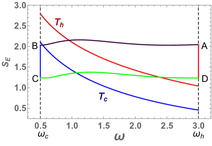
Figure 4: Typical frictionless refrigerator cycle ${\cal S}_{E}$ vs. $\omega$. Expansion adiabat $D\rightarrow C$. Cold isochore $C\rightarrow B$. Compression adiabat $B\rightarrow A$. Hot isochore $A\rightarrow D$. The hot and cold isotherms are indicated. The cycle parameters are $\omega_{c}=0.5,~{}T_{c}=1.5,~{}\omega_{h}=3,~{}T_{h}=3,~{}\tau_{c}=\tau_{h}=2.1,~{}|\mu|=0.5,\Gamma=1$.

The interplay between efficiency and cooling power is the main theme in the performance analysis. The efficiency of a refrigerator is defined by the coefficient of performance (COP):

$$COP=\frac{{\cal Q}_{c}}{\cal W}=\frac{\omega_{c}}{\omega_{h}-\omega_{c}}\leq\frac{T_{c}}{T_{h}-T_{c}}~{}.$$ (163)

The cooling power ${\cal R}_{c}$ is defined as:

$${\cal R}_{c}=\frac{{\cal Q}_{c}}{\tau_{cyc}}~{}.$$ (164)

Optimising the performance of the refrigerator can be carried out by a similar analysis to the one employed for the heat engine. Insight into the ideal performance can be gained by examining the expansion adiabat. The initial excitation should be minimized, requiring the hot bath to cool the working medium to its ground state. This is possible if $\hbar\omega_{h}\gg k_{B}T_{h}$. Next, the expansion should be as adiabatic as possible so that at the end the working medium is still as close as possible to its ground state $E_{C}\approx\frac{\hbar\omega_{c}}{2}$. The frictionless solutions found in Section IV.2 can be employed to achieve this task in minimum time.

V.3.1 Frictionless Refrigerator

The adiabatic refrigerator is obtained in the limit of infinite time $\mu\rightarrow 0$, leading to constant population $N$ and ${\cal S}_{E}$. Then, $E^{\bf C}=\frac{\omega_{c}}{\omega_{h}}E^{\bf D}$. At this limit, since $\tau\rightarrow\infty$, the cooling rate vanishes ${\cal R}_{c}=0$. The Carnot efficiency can be obtained when ${\cal C}=\frac{T_{h}}{T_{c}}$.

Frictionless solutions require that the state $\hat{\rho}$ is diagonal in energy in the beginning and at the end of the adiabat . The analytic propagator on the expansion adiabat (Equation (61)) describes the expansion adiabat: ${\bf D}\rightarrow{\bf C}$ :

$$E^{\bf C}=\frac{1}{{\cal C}}~{}\frac{1}{\Omega^{2}}\left(4-\mu^{2}c\right)\cdot E^{\bf D}~{},$$ (165)

where $c=\cos(\Omega\theta_{c})$ and $\theta_{c}=-\frac{1}{\mu}\log\left({\cal C}\right)$.

Frictionless points are obtained whenever $N^{\bf C}=N^{\bf D}$. The condition is $c=1$ in Equation (165). Then, $\mu<2$, leading to the critical frictional points (Equation (68)). These solutions have optimal efficiency Equation (163) with finite power. The optimal time allocated to the adiabat becomes (cf. Equation (69)) $\tau_{hc}^{*}=(1-{\cal C})/(\mu^{*}\omega_{h})$.

This frictionless solution with a minimum time allocation $\tau_{hc}^{*}$ scales as the inverse frequency $\omega_{c}^{-1}$, which outperforms the linear ramp solution $\omega(t)=\omega_{i}+gt$.

Other faster frictionless solutions can be obtained using the protocols of Section IV.2, such as the superadiabatic protocol or by applying optimal control theory Salamon et al. (2009). Both cases lead to the scaling of the adiabatic expansion time as $\tau_{hc}\propto\frac{1}{\sqrt{\omega_{c}\omega_{h}}}$.

Once the time allocation on the adiabats is set, the time allocation on the isochores is optimised for the thermalisation using the method of Rezek and Kosloff (2006), and the optimal cooling power becomes:

$${\cal R}_{c}^{*}~{}~{}=~{}~{}\frac{e^{z}}{(1+e^{z})^{2}}\Gamma\hbar\omega_{c}(N_{c}^{eq}-N_{h}^{eq})~{},$$ (166)

where $z=\Gamma_{h}\tau_{h}=\Gamma_{c}\tau_{c}$. The optimal $z$ is determined by the solution of the equation $2z+\Gamma(\tau_{hc}+\tau_{ch})=2\sinh(z)$.

V.3.2 The Sudden Refrigerator

Short adiabats generally lead to the excitation of the oscillator and result in friction (cf. Section IV.2). Nevertheless, a refrigerator can still operate at the limit of vanishing cycle time. In a similar fashion to the sudden engine, coherence can be exploited and leads to a finite cooling power when $\tau_{cyc}\rightarrow 0$. The cooling power for the sudden limit becomes:

$${\cal R}_{c}=-\hbar\omega_{c}\Gamma\left(N_{c}^{eq}-\frac{1}{2{\cal C}}(1+{\cal C}^{2})N_{h}^{eq}\right)~{}.$$ (167)

Note that the cooling rate in this sudden-limit becomes zero at a sufficiently low cold bath temperature so that $N_{c}^{eq}=(1+{\cal C}^{2})N_{h}^{eq}$. This formula loses its meaning and should not be used below this temperature.

V.3.3 The Quest to Reach Absolute Zero

The quantum harmonic refrigerator can serve as a primary model to explore cooling at very low temperatures. A necessary condition is that the internal temperature of the oscillator (Equation (34)) should be lower than the cold bath. $T_{int}<T_{c}$ when $T_{c}\rightarrow 0$. This condition imposes very high compression ratios ${\cal C}\gg\frac{T_{h}}{T_{c}}$ so that at point $D$ (cf. Figure 4), at the end of the hot thermalization, the oscillator is very close to the ground state.

An important feature of the model is that the cooling power vanishes as $T_{c}$ approaches zero. Qualitatively, ${\cal R}_{c}\rightarrow 0$ means that the adiabatic expansion from point $D\rightarrow C$ for high compression ratios requires a significant amount of time. Another issue is the rate of cold thermalisation $C\rightarrow B$ and its scaling with $T_{c}$ when the oscillator extracts heat from the cold bath. These issues can be made quantitative by exploring the scaling exponent $\alpha$ of the optimal cooling power with the cold bath temperature $T_{c}$:

$${\cal R}_{c}=\frac{{\cal Q}_{c}}{\tau_{cyc}}\propto T_{c}^{1+\alpha}~{}.$$ (168)

The vanishing of the cooling power ${\cal R}_{c}$ as $T_{c}\rightarrow 0$ is related to a dynamical version of the third-law of thermodynamics Levy et al. (2012); Kosloff (2013).

Walther Nernst formulated two independent formulations of the third-law of thermodynamics W. Nernst (1906a, b, 1918). The first is a purely static (equilibrium) one, also known as the “Nernst heat theorem”, phrased:

• The entropy of any pure substance in thermodynamic equilibrium approaches zero as the temperature approaches zero.

The second formulation is dynamical, known as the unattainability principle P. T. Landsberg (1956, 1989); Wheeler (1991); Belgiorno (2003); Levy et al. (2012):

• It is impossible by any procedure—no matter how idealised—to reduce any assembly to absolute zero temperature in a finite number of operations W. Nernst (1918).

The second law of thermodynamics already imposes a restriction on $\alpha$ Kosloff et al. (2000); Levy et al. (2012); Kosloff (2013). In steady-state, the entropy production rate is positive. Since the process is cyclic, it takes place only in the baths: $\sigma=\dot{\cal S}_{c}+\dot{\cal S}_{h}\geq 0$. When the cold bath approaches the absolute zero temperature, it is necessary to eliminate the entropy production divergence at the cold side because $\dot{\cal S}_{c}=\frac{{\cal R}_{c}}{T_{c}}$. Therefore, the entropy production at the cold bath when $T_{c}\rightarrow 0$ scales as:

$$\dot{\cal S}_{c}\sim-T_{c}^{\alpha}~{},~{}~{}~{}~{}\alpha\geq 0~{}.$$ (169)

For the case when $\alpha=0$, the fulfillment of the second-law depends on the entropy production of the other baths, which should compensate for the negative entropy production of the cold bath. The first formulation of the third-law slightly modifies this restriction. Instead of $\alpha\geq 0$, the third-law imposes $\alpha>0$, guaranteeing that the entropy production at the cold bath is zero at absolute zero: $\dot{S}_{c}=0$. This requirement leads to the scaling condition of the heat current ${\cal R}_{c}\sim T_{c}^{\alpha+1}~{},~{}~{}\alpha>0$.

The second formulation of the third-law is a dynamical one, known as the unattainability principle: no refrigerator can cool a system to absolute zero temperature at finite time. This formulation is more restrictive, imposing limitations on the system bath interaction and the cold bath properties when $T_{c}\rightarrow 0$ Levy et al. (2012). The rate of temperature decrease of the cooling process should vanish according to the characteristic exponent $\zeta$:

$$\frac{dT_{c}(t)}{dt}\sim-T_{c}^{\zeta},~{}~{}~{}T_{c}\rightarrow 0~{}~{}.$$ (170)

In order to evaluate Equation (170), the heat current can be related to the temperature change:

$${\cal J}_{c}(T_{c}(t))=-c_{V}(T_{c}(t))\frac{dT_{c}(t)}{dt}~{}.$$ (171)

This formulation takes into account the heat capacity $c_{V}(T_{c})$ of the cold bath. $c_{V}(T_{c})$ is determined by the behaviour of the degrees of freedom of the cold bath at low temperature. Therefore, the scaling exponents can be related $\zeta=1+\alpha-\eta$, where $c_{V}\sim T_{c}^{\eta}$ when $T_{c}\rightarrow 0$.

The harmonic quantum refrigerator is a primary example to explore the emergence of quantum dynamical restrictions that result in cooling power consistent with the third-law of thermodynamics. Analysis of the adibatic expansion will lead to insight on the cooling rate ${\cal R}_{c}$ and the exponent $\alpha$.

The frictionless solutions lead to an upper bound on the optimal cooling rate (Equation (164)). For the limit $T_{c}\rightarrow 0$, $\Gamma\tau_{hc}$ is large; therefore, $z$ is large, leading to:

$${\cal R}_{c}^{*}~{}\approx~{}\frac{\Gamma(\tau_{hc}+\tau_{ch})}{(1+\Gamma\tau_{hc})^{2}}\Gamma\hbar\omega_{c}(N_{c}^{eq}-N_{h}^{eq})~{}.$$ (172)

At high compression ratio, $N_{h}^{eq}\rightarrow 0$, and in addition $\omega_{c}\ll\Gamma$ one obtains:

$${\cal R}_{c}^{*}~{}\approx~{}\frac{1}{\tau_{hc}}\Gamma\hbar\omega_{c}N_{c}^{eq}~{}.$$ (173)

Optimizing ${\cal R}_{c}$ with respect to $\omega_{c}$ leads to a linear relation between $\omega_{c}$ and $T_{c}$, $\hbar\omega_{c}=k_{B}T_{c}$; therefore:

$${\cal R}_{c}\leq A\omega^{\nu}N_{c}^{eq}~{},$$ (174)

where $A$ is a constant and the exponent $\nu$ is either $\nu=2$ for the $\mu=const$ solution or $\nu=\frac{3}{2}$ for the optimal control solution. Therefore:

$${\cal R}_{c}^{*}~{}\approx~{}\hbar\omega_{c}^{2}N_{c}^{eq}$$ (175)

for the $\mu=const$ frictionless solution, and

$${\cal R}_{c}^{*}~{}\approx~{}\frac{1}{2}\hbar\omega_{c}^{\frac{3}{2}}\sqrt{\omega_{h}}N_{c}^{eq}$$ (176)

for the optimal control frictionless solution. Due to the linear relation between $\omega_{c}$ and $T_{c}$, Equations (175) and (176) determine the exponent $\alpha$, where $\alpha=1$ for the frictionless scheduling with constant $\mu$, and $\alpha=\frac{1}{2}$ for the optimal control frictionless scheduling. In all cases, the dynamical version of Nernst’s heat law is observed based only on the adiabatic expansion.

If one is forced to spend less time on the adiabat than the minimal time required for a shortcut solution, the oscillator cannot reach arbitrarily low energies or temperatures at the end of the expansion Stefanatos et al. (2010); Stefanatos (2016). At the limit, one approaches the sudden adiabat limit. In this case, the refrigerator cannot cool below a minimal ($T_{c}^{*}>0$) temperature, and the refrigerator thus satisfies the unattainability principle trivially.

The unattainability principle is related to the scaling of the heat transport $\Gamma_{c}$ with $T_{c}$. This issue has been explored in Levy et al. (2012); Kosloff (2013), and is related to the scaling of the heat conductivity with temperature. The arguments of Levy et al. (2012) are applicable to the quantum harmonic refrigerator.

VI Overview

Learning from example has been one of the major sources of insight in the study of thermodynamics. A good example can bridge the gap between concrete and abstract theory. The harmonic oscillator quantum Otto cycle serves as a primary example of a quantum thermal device inspiring experimental realisation Roßnagel et al. (2016); Blickle and Bechinger (2012). On the one hand, the model is very close to actual physical realisations in many scenarios Zhang et al. (2014). On the other hand, many features of the model can be obtained as closed-form analytic solutions.

Many of the features obtained for the quantum harmonic Otto engine have been observed in stochastic thermodynamics Seifert (2012); Derényi and Astumian (1999); Hondou and Sekimoto (2000); Schmiedl and Seifert (2007); Blickle and Bechinger (2012). The analytic properties of the harmonic oscillator—in particular, the Gaussian form of the state—have motivated studies of classical stochastic models of harmonic heat engines Raz et al. (2016); Blickle and Bechinger (2012); Dechant et al. (2016). When comparing the two theories, the results seem identical in many cases. Observing the Heisenberg equations of motion for the thermodynamical variables, $\hbar$ does not appear. Planck’s constant in the commutators is cancelled by the inverse Planck constant in the equation of motion. This raises the issue of what is quantum in the quantum harmonic oscillator, or a related issue—what is quantum in quantum thermodynamics Vinjanampathy and Anders (2016)?

In this review, we emphasized the power of the generalized Gibbs state in allowing a concise description of an out-of-equilibrium situation of non-commuting operators. Using properties of Lie algebra of operators, we could obtain a dynamical description of the state based on only three variables: ${\bm{\mathrm{\hat{H}}}}$, ${\bm{\mathrm{\hat{L}}}}$, and ${\bm{\mathrm{\hat{C}}}}$. In the spirit of open quantum systems, we could describe the cycle propagator as a catenation of stroke propagators. All these propagators were cast in the framework of the operator algebra, showing the power of Heisenberg representation. The quantum variables were chosen to have direct thermodynamical relevance as energy and coherence. In this review, we emphasized the connections between the algebraic approach and other popular methods that have been employed to obtain insight on the harmonic engine.

This formalism allows the cycles to be classified according to the role of coherence. If the coherence vanishes at the points where the strokes meet, frictionless cycles are obtained. Such cycles require special scheduling of $\omega(t)$ so that the coherence generated at the beginning of the stroke can be cashed upon at the end. We reviewed the different approaches to obtain such scheduling and the minimum time that such moves can be generated. This period is related to quantum speed limits Mandelstam and Tamm (1945); Margolus and Levitin (1998); Giovannetti et al. (2003); Deffner and Lutz (2013); Levy et al. (2016), which are in turn related to the energy resources available to the system. We chose the geometric mean $\tau_{a}\propto 1/\sqrt{\omega_{h}\omega_{c}}$ to represent the minimum time allocation. Faster scheduling requires unreasonable constraints on the stored energy in the oscillator during the stroke. We also assume that this extra energy required to achieve the fast control is not dissipated and can be accounted for as a catalyst.

For these frictionless solutions on the adiabats, the optimal time allocation for thermalisation is finite, leading to incomplete thermalisation. This allows the minimum cycle time for frictionless cycles to be estimated. Avoiding friction completely is an ideal that practically cannot be obtained. Using a simple noise model, we show that some friction will always be present.

The model demonstrates the fundamental tradeoff between efficiency and power. The frictionless solutions are a demonstration that quantum coherence which is related to friction can be cashed upon, using interference to cancel this friction. As a result, the maximum efficiency of the engine can be obtained in finite cycle time. Nevertheless, the Otto efficiency is smaller than the reversible Carnot efficiency $\eta_{o}=1-\frac{\omega_{c}}{\omega_{h}}\leq\eta_{c}=1-\frac{T_{c}}{T_{h}}$, and operating at the Carnot efficiency will lead to zero power. The entropy production can be associated with the heat transport, and for this case the entropy production is linearly related to the power. Maximum power also implies maximum entropy production. This finding is consistent with the study of Shiraishi et al. Shiraishi et al. (2016). Any finite power cycle requires out-of-equilibrium setups that lead to dissipation. In the sudden limit, there is no reversible choice. Even at zero power the entropy production is positive. This could be the cost of maintaining coherence.

Beyond a minimum time allocation on the adiabats $\tau_{a}$, friction cannot be avoided. The transition point is the exceptional point of the non-hermitian degeneracy on the adiabatic propagator Uzdin et al. (2013). These short time cycles are in the realm of the sudden cycles. The sudden cycles are an example of an engine or refrigerator with no classical analogue. Power production requires coherence. A sudden model without coherence operates as a dissipator generating entropy on both the hot and cold baths. The sudden cycle is composed of non-commuting propagators with small action. Such cycles are universal and have a common continuous limit Uzdin et al. (2015, 2016). In the continuous limit, friction and heat leaks cannot be avoided Correa et al. (2015); Plastina et al. (2014).

An obvious direction to look for quantum effects is to go to low temperatures where the unit of energy changes from $k_{B}T$ to $\hbar\omega$. The adiabatic expansion is the bottleneck for cooling to extremely low temperatures. The zero point energy plays an important role. We can approach the ground state on the hot side by increasing the frequency, leading to the minimal initial energy $E_{A}=\frac{1}{2}\hbar\omega_{h}$. This is a large amount of energy compared to the cold side, which has to be eliminated adiabatically or by using frictionless protocols. Any small error in these protocols will null the cooling.

The Otto quantum refrigerator is a good example for gaining insight into the limits of cooling when operating at extremely low temperatures. Such refrigerators are an integral part of any quantum technology. In the reciprocating Otto cycle, the cooling power is restricted either by the adiabatic expansion or by vanishing of the heat transport when $T_{c}\rightarrow 0$ Levy et al. (2012). The adiabatic expansion time is an intrinsic property of the working medium. For optimal frictionless solutions, it scales as $\tau_{hc}=O(T_{c}^{\frac{1}{2}})$, which gives a maximum rate of entropy production $\sigma=O(T_{c}^{\frac{1}{2}})$, thus vanishing when $T_{c}\rightarrow 0$. This is a demonstration of a dynamical version of the Nernst heat law Rezek et al. (2009); Levy et al. (2012); Kosloff (2013).

The quantum harmonic Otto cycle has been a template for many models of quantum heat devices due to its analytic properties—for example, Otto cycles with interacting particles Wang et al. (2015); Jaramillo et al. (2016) or operating with many modes Terças et al. (2017). The protocols developed for the harmonic case are generalised to eliminate friction in many-body dynamics.

The quantum harmonic Otto cycle has been a source of inspiration for theory and experiment. The model incorporates generic features of irreversible operation which includes friction and heat transport. The system can bridge the conceptual gap between a single microscopic device to a macroscopic heat engine.