CMB anomalies and the effects of local features of the inflaton potential

Abstract

Recent analysis of the WMAP and Planck data have shown the presence of a dip and a bump in the spectrum of primordial perturbations at the scales $k=0.002$ Mpc^-1 and $k=0.0035$ Mpc^-1 respectively. We analyze for the first time the effects a local feature in the inflaton potential to explain the observed deviations from scale invariance in the primordial spectrum. We perform a best fit analysis of the cosmic microwave background (CMB) radiation temperature and polarization data. The effects of the features can improve the agreement with observational data respect to the featureless model. The best fit local feature affects the primordial curvature spectrum mainly in the region of the bump, leaving the spectrum unaffected on other scales.

I Introduction

There are important observational motivations to study modifications of the inflaton potential, like the observed deviations of the spectrum of primordial curvature perturbations from a power law spectrum  Gariazzo:2014dla ; Hazra:2014jwa ; Hunt:2013bha ; Mukherjee:2003cz ; Mukherjee:2003ag ; Bridle:2003sa ; Hazra:2013nca ; Vazquez:2013dva ; Hannestad:2000pm ; Bridges:2008ta ; Hazra:2014aea ; Gauthier:2012aq ; dePutter:2014hza ; Ade:2015lrj ; Planck:2013jfk ; DiValentino:2016ikp ; Benetti:2016tvm ; Chen:2016vvw ; Xu:2016kwz ; Chen:2016zuu ; Hazra:2016fkm . In Refs. Gariazzo:2014dla ; Hazra:2014jwa ; Hunt:2013bha ; Mukherjee:2003cz ; Mukherjee:2003ag ; Bridle:2003sa ; Hazra:2013nca ; Vazquez:2013dva ; Hannestad:2000pm ; Bridges:2008ta ; Hazra:2014aea ; Gauthier:2012aq ; dePutter:2014hza the authors study the effects of analizing the cosmic microwave background (CMB) radiation using a free function for the spectrum of primordial scalar perturbations, i.e., they do not consider the usual power law spectrum predicted by most of the simplest inflationary models encyclopaedia ; Ade:2015lrj ; Planck:2013jfk . For example, the primordial spectrum can be parametrized with wavelets Mukherjee:2003cz ; Mukherjee:2003ag , linear interpolation Bridle:2003sa ; Hazra:2013nca ; Vazquez:2013dva , interpolating spline functions Hazra:2014aea ; Gauthier:2012aq ; dePutter:2014hza , among other methods Gariazzo:2014dla ; DiValentino:2016ikp .

Some interesting evidence of these deviations were given in Gariazzo:2014dla ; DiValentino:2016ikp where it was used a method based on a “piecewise cubic Hermite interpolating polynomial” (PCHIP) for the primordial power spectrum. This analysis showed that the spectrum of primordial perturbations can be approximated with a power law in the range of values $0.007\mbox{ Mpc}^{-1}<k<0.2\mbox{ Mpc}^{-1}$ while in the range $0.001\mbox{ Mpc}^{-1}<k<0.0035\mbox{ Mpc}^{-1}$ there are a dip and a bump at $k=0.002$ Mpc^-1 and $k=0.0035$ Mpc^-1, with a statistical significance of about $2\sigma$ and $1\sigma$, respectively. Similar results were reported in several other analyses Shafieloo:2003gf ; Nicholson:2009pi ; Hazra:2013ugu ; Hazra:2014jwa ; Nicholson:2009zj ; Hunt:2013bha ; Hunt:2015iua ; Goswami:2013uja ; Matsumiya:2001xj ; Matsumiya:2002tx ; Kogo:2003yb ; Kogo:2005qi ; Nagata:2008tk ; Ade:2015lrj ; Gariazzo:2014dla ; DiValentino:2015zta using different techniques and both the WMAP wmapfmr and Planck pi ; Adam:2015rua measurements. In this paper we study how local features of the inflaton potential can model this type of local glitches of the spectrum of primordial curvature perturbations. We also study the effects of these features on the primordial tensorial perturbation spectrum.

Features of the inflaton potential can affect the evolution of primordial curvature perturbations GallegoThesis ; Cadavid:2015iya ; Gariazzo:2014dla ; Motohashi:2015hpa ; et ; aer ; a1 ; a2 ; a3 ; Adams ; Chluba:2015bqa ; Chen:2011zf ; Palma:2014hra ; starobinsky ; constraints1 ; constraints2 ; Hazra:2014jka ; Hazra:2014goa ; Martin:2014kja ; Romano:2014kla ; Ashoorioon:2006wc ; Ashoorioon:2008qr ; Cai:2015xla and consequently generate a variation in the amplitude of the spectrum and bispectrum GallegoThesis ; Cadavid:2015iya ; Motohashi:2015hpa ; et ; aer ; a1 ; a2 ; a3 ; Adams ; Romano:2014kla . This can provide a better fit of the observational data in the regions where the spectrum shows some deviations from a power law Motohashi:2015hpa ; et ; constraints1 ; constraints2 ; a1 ; a2 ; a3 ; Adams ; Gariazzo:2014dla ; Hazra:2014jwa ; Hunt:2013bha ; Joy:2007na ; Joy:2008qd ; Mortonson:2009qv . In this paper we perform a best fit analysis of the CMB radiation temperature and polarization data and we study the effects of a local feature of the inflation potential which affects the primordial curvature spectrum in the region of the bump.

II Local features

We consider a single scalar field minimally coupled to gravity with a standard kinetic term according to the action

$$S=\int d^{4}x\sqrt{-g}\left[\frac{1}{2}M^{2}_{Pl}R-\frac{1}{2}g^{\mu\nu}\partial_{\mu}\phi\partial_{\nu}\phi-V(\phi)\right],$$ (1)

where $M_{Pl}=(8\pi G)^{-1/2}$ is the reduced Planck mass and $g_{\mu\nu}$ is the flat $FLRW$ metric. The Friedmann equation and the equation of motion of the inflaton are obtained from the variation of the action with respect to the metric and the scalar field respectively

$$H^{2}\equiv\left(\frac{\dot{a}}{a}\right)^{2}=\frac{1}{3M^{2}_{Pl}}\left(\frac{1}{2}\dot{\phi}^{2}+V(\phi)\right),$$ (2)

$$\ddot{\phi}+3H\dot{\phi}+\partial_{\phi}V=0,$$ (3)

where $H$ is the Hubble parameter, and dots and $\partial_{\phi}$ denote derivatives with respect to time and scalar field respectively. The slow-roll parameters are defined

$$\epsilon\equiv-\frac{\dot{H}}{H^{2}}\,\,\,\,,\,\,\,\,\eta\equiv\frac{\dot{\epsilon}}{\epsilon H}.$$ (4)

We consider a potential energy given by Cadavid:2015iya

$$V(\phi) = V_{0}(\phi)+V_{F}(\phi)\,,$$ (5)

$$V_{F}(\phi) = \lambda e^{-(\frac{\phi-\phi_{0}}{\sigma})^{2}}\,,$$ (6)

where $V_{0}(\phi)$ is the featureless potential and $V_{F}$ corresponds to a step symmetrically dumped by an even power negative exponential factor. In this paper we will consider the case of a quadratic inflaton potential

$$V_{0}(\phi)=\frac{1}{2}m^{2}\phi^{2}\,.$$ (7)

The tensor-to-scalar ratio for a monomial potential $\phi^{n}$ is $r\approx 16n/(4N_{e}+n)$, where $N_{e}$ is the number of $e$-folds before the end of inflation Ade:2015lrj ; Planck:2013jfk . In the case of quadratic inflation $r\approx 0.16$ for $N_{e}\approx 50$, which is not in good agreement with observational data. Our analysis confirms this when we fit data without the feature. We will show later that the effects of local features improve the agreement with CMB data but not enough to get a $\chi^{2}$ as low as the one of other inflationary models with lower values of $r$.

This type of modification of the slow-roll potential is called local feature (LF) Cadavid:2015iya which differs from the branch feature (BF) Cadavid:2015iya ; Romano:2014kla since the potential is symmetric with respect to the location of the feature and it is only affected in a limited range of the scalar field value. Due to this the spectrum and bispectrum are only modified in a narrow range of scales, in contrast to the BF in which there are differences in the power spectrum between large and small scale which are absent in the case of LF. In some cases the step in the spectrum due to a BF can be very small, and the difference between large and small scale effects would not make BF observationally distinguishable from LF. Nevertheless in general the oscillation patterns produce in the spectrum by a single BF would be different because a single LF can be considered as the combination of two appropriate BF Cadavid:2015iya .

In this paper we use the local type effect of these features to model phenomenologically local glitches of the primordial scalar spectrum on the scales $k=0.002\mbox{ Mpc}^{-1}$ and $k=0.0035\mbox{ Mpc}^{-1}$ Gariazzo:2014dla , and to study their effects on the primordial tensor spectrum, without affecting other scales.

The effects of the feature on the slow-roll parameters are shown in Fig. 1, where we can see that there are oscillations of the slow-roll parameters around the feature time $t_{0}$, defined as $\phi_{0}=\phi(t_{0})$ Cadavid:2015iya . The magnitude of the potential modification is controlled by the parameter $\lambda$, as its effect is such that larger value of $\lambda$ give larger values of the slow-roll parameters. The size of the range of field values where the potential is affected by the feature is determined by the parameter $\sigma$ and the slow-roll parameters are smaller for larger $\sigma$. We define $k_{0}$ as the scale exiting the horizon at the feature time $t_{0}$, $k_{0}=-1/\tau_{0}$, where $\tau_{0}$ is the value of conformal time corresponding to $t_{0}$. Oscillations occur around $k_{0}$, and their location can be controlled by changing $\phi_{0}$. We adopt a system of units in which $c=\hbar=M_{Pl}=1$.

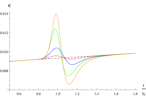
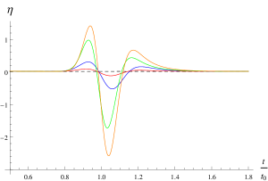
Figure 1: The numerically computed slow-roll parameters $\epsilon$ and $\eta$ around the feature time $t_{0}$ for $\lambda=-4\times 10^{-12},\sigma=0.05$, and $k_{0}=1.2\times 10^{-3}$ (blue), $\lambda=-10^{-12},\sigma=0.05$, and $k_{0}=1.3\times 10^{-3}$ (red), $\lambda=-10^{-11},\sigma=0.04$, and $k_{0}=1.3\times 10^{-3}$ (green), and $\lambda=-1.5\times 10^{-11},\sigma=0.04$, and $k_{0}=1.2\times 10^{-3}$ (orange). The dashed lines correspond to the featureless slow roll parameters.

III Spectrum of curvature tensor perturbations

In order to study the curvature perturbations we expand perturbatively the action with respect to the background $FLRW$ solution. The second order action for scalar perturbations in the comoving gauge takes the form m

$$S_{2} = \int dtd^{3}x\left[a^{3}\epsilon\dot{\zeta}^{2}-a\epsilon(\partial\zeta)^{2}\right]\,.$$ (8)

The equation for curvature perturbations $\zeta$ obtained from the Lagrange equations is

$$\frac{\partial}{\partial t}\left(a^{3}\epsilon\frac{\partial\zeta}{\partial t}\right)-a\epsilon\delta^{ij}\frac{\partial^{2}\zeta}{\partial x^{i}\partial x^{j}}=0.$$ (9)

Taking the Fourier transform and using conformal time $d\tau\equiv dt/a$ we get

$$\zeta^{\prime\prime}_{k}+2\frac{z^{\prime}}{z}\zeta^{\prime}_{k}+k^{2}\zeta_{k}=0,$$ (10)

where $k$ is the comoving wave number, $z\equiv a\sqrt{2\epsilon}$, and primes denote a derivative with respect to the conformal time. The two-point function of curvature perturbations is

$$\Braket{\hat{\zeta}(\vec{k}_{1},t)\hat{\zeta}(\vec{k}_{2},t)}\equiv(2\pi)^{3}\frac{2\pi^{2}}{k^{3}}P_{\zeta}(k)\delta^{(3)}(\vec{k}_{1}+\vec{k}_{2})\,,$$ (11)

where the power spectrum of curvature perturbations is defined as

$$P_{\zeta}(k)\equiv\frac{k^{3}}{2\pi^{2}}|\zeta_{k}|^{2}\,.$$ (12)

The effects of the features on the primordial scalar spectrum are plotted in Fig. 2 for different values of the parameters $\lambda,\sigma$, and $k_{0}$ Cadavid:2015iya . The spectrum of primordial curvature perturbations has oscillations around $k_{0}$, whose amplitude is larger for larger $\lambda$ since the latter controls the magnitude of the potential modification. The amplitude of the spectrum oscillations is larger for smaller $\sigma$, because in this case the change in the potential is more abrupt and consequently the slow-roll parameters are larger.

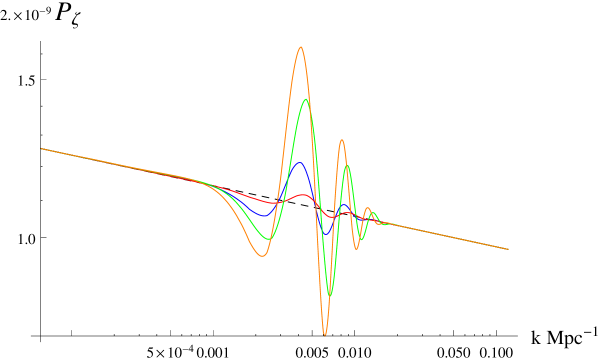
Figure 2: The power spectrum of primordial curvature perturbations $P_{\zeta}$ is plotted for $\lambda=-4\times 10^{-12},\sigma=0.05$, and $k_{0}=1.2\times 10^{-3}$ (blue), $\lambda=-10^{-12},\sigma=0.05$, and $k_{0}=1.3\times 10^{-3}$ (red), $\lambda=-10^{-11},\sigma=0.04$, and $k_{0}=1.3\times 10^{-3}$ (green), and $\lambda=-1.5\times 10^{-11},\sigma=0.04$, and $k_{0}=1.2\times 10^{-3}$ (orange). The dashed lines correspond to the featureless spectrum.

The equation for tensor perturbations can be derived in a way similar to the case of scalar perturbations, giving

$$h^{\prime\prime}_{k}+2\frac{a^{\prime}}{a}h^{\prime}_{k}+k^{2}h_{k}=0\,,$$ (13)

where again $k$ is the comoving wave number. The power spectrum of tensor perturbations is obtained from the two-point function as

$$P_{h}(k)\equiv\frac{2k^{3}}{\pi^{2}}|h_{k}|^{2}\,,$$ (14)

from which the tensor-to-scalar ratio can be defined as the ratio between the spectrum of tensor and scalar perturbations as

$$r\equiv\frac{P_{h}}{P_{\zeta}}\,.$$ (15)

The effects of the features on the primordial tensor spectrum are plotted in Fig. 3 for different values of the parameters $\lambda,\sigma$, and $k_{0}$.

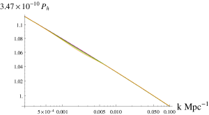
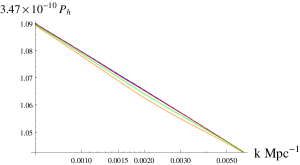
Figure 3: The power spectrum of primordial tensor perturbations $P_{h}$ is plotted for $\lambda=-4\times 10^{-12},\sigma=0.05$, and $k_{0}=1.2\times 10^{-3}$ (blue), $\lambda=-10^{-12},\sigma=0.05$, and $k_{0}=1.3\times 10^{-3}$ (red), $\lambda=-10^{-11},\sigma=0.04$, and $k_{0}=1.3\times 10^{-3}$ (green), and $\lambda=-1.5\times 10^{-11},\sigma=0.04$, and $k_{0}=1.2\times 10^{-3}$ (orange). The dashed lines correspond to the featureless spectrum. The plot on the right corresponds to a zoom of the left plot. As it can be seen the effects of the different features on the spectrum $P_{h}$ are rather small and the spectra of the models with features are difficult to distinguish from the featureless model spectrum.

These effects are not very significant and in fact the observational data analysis we will present in the rest of the paper confirms that local features affect mainly the curvature spectrum.

IV Effects of local features on the CMB spectrum

In Fig. 4 we show the effects of local features on the temperature (TT) CMB spectrum. Since we are considering a feature of local type, as theoretically expected, the spectrum is not affected on scales sufficiently far from $k_{0}$. Branch features Cadavid:2015iya could on the contrary also introduce a step in the power spectrum, modifying it also on scales far from $k_{0}$, and for this reason LF are more appropriate to model local deviations of the spectrum.

The main effects produced by the LF appear between $\ell=10$ and $\ell=100$ in the TT spectrum. They correspond to the wiggles of the primordial scalar fluctuations shown in Fig. 2. The class of LF we consider allows to fit the small bump at $\ell\simeq 40$ better than the dip at $\ell\simeq 20$ in the CMB spectrum. The impact of the LF on the BB spectrum is much smaller, since, as discussed previously, the effect of the feature on the primordial tensorial perturbations spectrum is negligible.

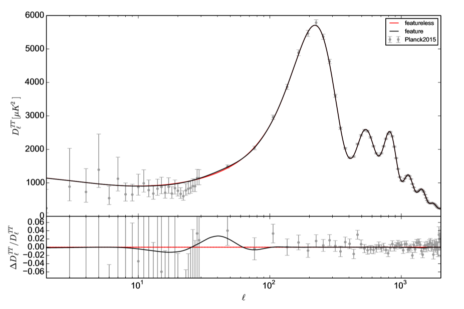
Figure 4: The $D_{l}^{TT}=\ell(\ell+1)C_{\ell}^{TT}/(2\pi)$ spectrum in units of $\mu K^{2}$ is plotted as a function of the multipole $l$. We compare the best-fit obtained using the inflationary model without feature (red line) to the one obtained introducing the local feature (black line). In the lower panel we plot the relative difference with respect to the featureless case. The data points are from the 2015 Planck release Adam:2015rua . The cosmological parameters used to compute the two spectra are reported in Tab. 1.

IV.1 The observational data analysis method

To study the effects produced by local features on the CMB spectrum, we modified the Boltzmann code CAMB Lewis:1999bs that computes the theoretical spectra and the corresponding Markov Chain Monte Carlo (MCMC) code CosmoMC Lewis:2002ah in order to use a non-standard power spectrum for the primordial curvature perturbations.

As a base model we considered the standard parameterization of the $\Lambda$CDM model for the evolution of the universe, that includes four parameters: the current energy density of baryons and of Cold Dark Matter (CDM) $\Omega_{b}h^{2}$ and $\Omega_{c}h^{2}$, the ratio between the sound horizon and the angular diameter distance at decoupling $\theta$, and the optical depth to reionization $\tau$.

The parameterization of the primordial power spectra is modified to take into account the presence of the local feature. To see the effects of the feature, we compare the results obtained in the featureless model with the ones obtained when a local feature is added. The comparison of the effects of LF of different inflationary potentials is left for future studies.

The data sets that we use to test the LF are taken from the last release from the Planck Collaboration Adam:2015rua for the temperature and E-mode polarization modes. We consider the temperature and polarization power spectra in the range $2\leq\ell\leq 29$ (low-$\ell$) and only the temperature power spectrum at higher multipoles, $30\leq\ell\leq 2500$ (high-$\ell$). Since the polarization spectra at high multipoles are still under discussion and some residual systematics were detected by the Planck Collaboration Aghanim:2015xee ; Ade:2015xua , we do not include the full polarization spectra obtained by Planck. Moreover, we do not include the data on the BB spectrum as obtained from the Bicep2/Keck collaboration Ade:2015fwj , because the baseline inflationary model that we consider ($\phi^{2}$) cannot reproduce the small amount of primordial tensor modes that are observed after cleaning the Bicep2/Keck data using the polarized dust emission obtained by the high frequency maps by Planck Ade:2015tva .

V Results

Parameter	with feature	featureless
$10^{2}\omega_{b}$	$2.203\pm 0.019$	$2.203\pm 0.019$
$\omega_{c}$	$0.122\pm 0.001$	$0.121\pm 0.001$
$\theta$	$1.0406\pm 0.0004$	$1.0406\pm 0.0004$
$\tau$	$0.059\pm 0.015$	$0.059\pm 0.016$
$\ln(10^{10}A_{s})$	$3.056\pm 0.031$	$3.054\pm 0.032$
$H_{0}$	$66.4\pm 0.5$	$66.5\pm 0.5$
$-10^{12}\lambda$	$[0.05,1.23)$ $\{1.12\}$	-
$10^{2}\sigma$	$5.3\,^{+1.1}_{-3.1}$	-
$10^{3}k_{0}$	$[1.0,1.3)$ $\{1.13\}$	-
$\chi^{2}_{\text{Planck low-}\ell}$	10505.31	10504.92
$\chi^{2}_{\text{Planck high-}\ell}$	764.90	767.8
$\chi^{2}_{\text{nuisance priors}}$	1.08	0.27
$\chi^{2}_{tot}$	11271.29	11273.0

Table 1: Constraints on the cosmological parameters and $\chi^{2}$ for the model with and without feature. All the constraints are given at 1$\sigma$ confidence level. The lower limits on the feature parameters correspond to the limits we used as a prior. The best fit are values inside curly brackets. We separately report the different contributions to the $\chi^{2}$ (Planck low-$\ell$, Planck high-$\ell$ and from the priors on the nuisance parameters) and the total.

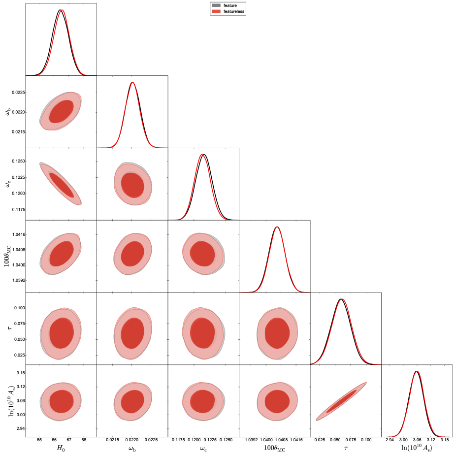
Figure 5: A comparison between the model with and without features is given for the parameters $H_{0}$, $\omega_{b}$, $\omega_{c}$, $\theta$, $\tau$ and $\ln(10^{10}A_{s})$. All the results are obtained considering the Planck low-$\ell$+high$\ell$ data combination. As can be seen the effects of the feature on the estimation of these non inflationary cosmological parameters is negligible.

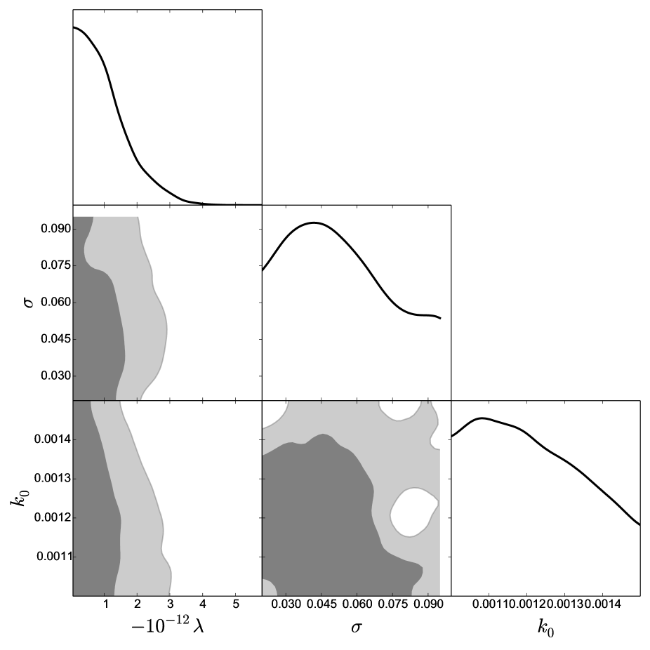
Figure 6: The results of the data fitting analysis for the parameters $\lambda$, $\sigma$ and $k_{0}$ are shown for the model with local features.

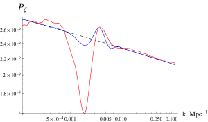
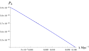
Figure 7: The numerically computed spectrum of the primordial curvature fluctuations $P_{\zeta}$ and of the tensor perturbations $P_{h}$ are plotted for the best fit values in Tab. 1: $\lambda=-1.12\times 10^{-12},\sigma=0.053$, and $k_{0}=1.13\times 10^{-3}$ (blue). On the left, the red lines correspond to the best-fit reconstructed primordial power spectrum from Ref. DiValentino:2016ikp . The dashed lines correspond to the featureless spectrum.

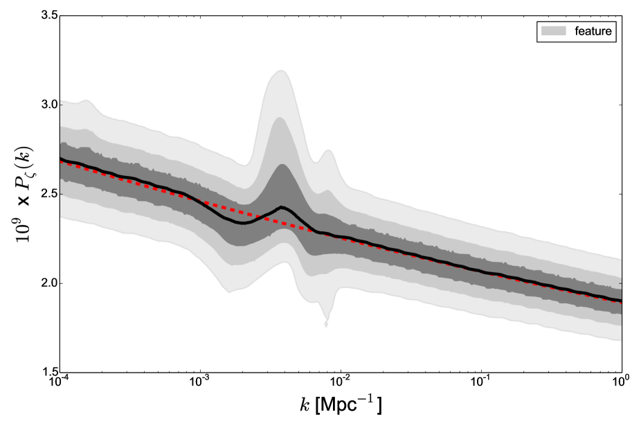
Figure 8: The 1, 2 and 3$\sigma$ constraints obtained from observational data analysis are plotted for the primordial curvature perturbations spectrum for the model with local features. The spectrum for the featureless model is plotted with a red line.

The results of the data fitting analysis are reported in Tab. 1 and in Figs. 5 to 8.

In Tab. 1 we show the best-fit values written inside brackets and the 1$\sigma$ constraints of the parameters. It should be noted that the bounds we obtain are more stringent than the Planck ones because $n_{s}$ is not a free parameter. Fixing the value of scalar spectral index reduces the confidence ranges for the others parameters, and consequently our bounds are smaller. If we had left free the potential of the inflaton in a generic monomial form $V_{0}\sim\phi^{n}$, then we could have obtained larger bounds as in the Planck team analysis where $n_{s}$ is a free parameter. This could be done in a future work, but it goes beyond the scope of the present paper.

Comparing the results obtained with and without feature we can see that the presence of the LF has no impact on the background cosmological parameters. This is clear from the marginalized 1D and 2D plots in Fig. 5. The effect of the feature is evident around the location of the bump of the CMB temperature spectrum (see Fig. 4), and it corresponds to an improvement of the total $\chi^{2}$. As reported in Tab. 1, the improvement comes from the $\chi^{2}$ of the low-$\ell$ Planck likelihood. Our analysis cannot be compared with the Planck results Ade:2015xua ; Ade:2015tva , we are assuming the $\phi^{2}$ inflationary model instead of using a phenomenological approach with independent $n_{s}$ and $r$. Quadratic inflation corresponds to high values of $r$ which are not in agreement with the Planck best-fit model obtained using $n_{s}$ and $r$ as independent parameters. The effects of the feature improve the $\chi^{2}$ with respect to the featureless $\phi^{2}$ case, but this improvement is not large enough to make it competitive with other models. Nevertheless, the same LF could be applied to other inflationary scenarios to produce an analogous improvement of the $\chi^{2}$. The analyses of the effects of the LF for inflationary models that are in better agreement with the observed CMB spectra are left for future studies.

In Fig. 6 we show the 1D marginalized posterior distributions and the correlations between the feature parameters. From the correlation plot between $\lambda$ and $k_{0}$ we can see that the size of the feature can be larger if the feature is located at a smaller wavemode $k_{0}$. This is because the CMB temperature spectrum does not allow any wiggles above $\ell\simeq 60$, thus limiting the amplitude of the feature. The 2D plots for the parameter $\sigma$ seem to show that there is no lower bound on it. This is not in tension with the 1$\sigma$ constraints on the $\sigma$ parameter reported in Tab. 1, because of volume effects that occur in the Bayesian marginalization procedure. The preference for a non-minimum value of $\sigma$ is mild, indeed there is no lower bound at 2$\sigma$ confidence level.

The constraints on the primordial scalar spectrum are shown in Figs. 7 and 8. In the left panel of Fig. 7 we compare the best-fit primordial power spectrum of scalar perturbations obtained in our analysis (blue) and the reconstructed one from Ref. DiValentino:2016ikp . The comparison underlines how a local feature can reproduce the behaviour of the primordial spectrum, but further studies, which will be presented in some future work, on the feature potential are required in order to obtain a perfect agreement. The right panel of the same Fig. 7 shows that the effect of the feature is very small in the tensor spectrum. In Fig. 8 we plot the marginalized constraints on the primordial scalar spectrum. The 1, 2, and 3$\sigma$ bands refer to the model with LF, while the solid black line shows the corresponding best-fit spectrum, computed from the entire set of primordial spectra obtained from the MCMC scan. The red dashed line shows the spectrum obtained for the same cosmological parameters but without the feature. From the figures we can note that the effects that the LF brings are more important for the scalar spectrum, while they are negligible for the tensor spectrum. For this reason, we do not show the same plot as for Fig. 8 for the tensor spectrum.

VI Conclusions

We have studied the effects of local features in the inflaton potential on the spectra of primordial curvature perturbations and their impact on the temperature anisotropies of the CMB. In order to study the effects on the CMB spectrum we have modified the CAMB and CosmoMC codes in order to use a non-standard power-law power spectrum for the primordial perturbations, to take into account the presence of the local feature. We have performed a best fit analysis of CMB temperature and polarization data from Planck. We have found no significant effects on cosmological parameters related to the propagation of CMB photons after decoupling, while LF improve the fit of the CMB temperature and polarization data. We have also confirmed the theoretical expectation that local features do not affect the primordial power spectrum at scales far from the characteristic scale $k_{0}$, which leaves the horizon around the feature time.

In the future it will be interesting to analyze the effects of local features in order to explain other deviations of the CMB spectrum, such as for example the anomalies occurring around $l\approx 800$ Hazra:2014jwa . It will also be important to study the effects of LF in inflationary models with different featureless $V_{0}$ potentials, and to compare them to the effects of branch features.

- (1) S. Gariazzo, C. Giunti, and M. Laveder, JCAP 1504, 023 (2015), arXiv:1412.7405.
- (2) D. K. Hazra, A. Shafieloo, and T. Souradeep, JCAP 1411, 011 (2014), arXiv:1406.4827.
- (3) P. Hunt and S. Sarkar, JCAP 1401, 025 (2014), arXiv:1308.2317.
- (4) P. Mukherjee and Y. Wang, Astrophys. J. 593, 38 (2003), arXiv:astro-ph/0301058.
- (5) P. Mukherjee and Y. Wang, Astrophys. J. 599, 1 (2003), arXiv:astro-ph/0303211.
- (6) S. L. Bridle, A. M. Lewis, J. Weller, and G. Efstathiou, Mon. Not. Roy. Astron. Soc. 342, L72 (2003), arXiv:astro-ph/0302306.
- (7) D. K. Hazra, A. Shafieloo, and G. F. Smoot, JCAP 1312, 035 (2013), arXiv:1310.3038.
- (8) J. A. Vazquez, M. Bridges, Y.-Z. Ma, and M. P. Hobson, JCAP 1308, 001 (2013), arXiv:1303.4014.
- (9) S. Hannestad, Phys. Rev. D63, 043009 (2001), arXiv:astro-ph/0009296.
- (10) M. Bridges, F. Feroz, M. P. Hobson, and A. N. Lasenby, Mon. Not. Roy. Astron. Soc. 400, 1075 (2009), arXiv:0812.3541.
- (11) D. K. Hazra, A. Shafieloo, G. F. Smoot, and A. A. Starobinsky, JCAP 1406, 061 (2014), arXiv:1403.7786.
- (12) C. Gauthier and M. Bucher, JCAP 1210, 050 (2012), arXiv:1209.2147.
- (13) R. de Putter, E. V. Linder, and A. Mishra, Phys. Rev. D89, 103502 (2014), arXiv:1401.7022.
- (14) Planck Collaboration, P. Ade et al., (2015), arXiv:1502.02114.
- (15) Planck Collaboration, P. Ade et al., (2013), arXiv:1303.5082.
- (16) E. Di Valentino, S. Gariazzo, M. Gerbino, E. Giusarma, and O. Mena, Phys. Rev. D93, 083523 (2016), arXiv:1601.07557.
- (17) M. Benetti and J. S. Alcaniz, Phys. Rev. D94, 023526 (2016), arXiv:1604.08156.
- (18) X. Chen, C. Dvorkin, Z. Huang, M. H. Namjoo, and L. Verde, JCAP 1611, 014 (2016), arXiv:1605.09365.
- (19) Y. Xu, J. Hamann, and X. Chen, (2016), arXiv:1607.00817.
- (20) X. Chen, P. D. Meerburg, and M. Münchmeyer, JCAP 1609, 023 (2016), arXiv:1605.09364.
- (21) D. K. Hazra, A. Shafieloo, G. F. Smoot, and A. A. Starobinsky, JCAP 1609, 009 (2016), arXiv:1605.02106.
- (22) J. Martin, C. Ringeval, and V. Vennin, (2013), arXiv:1303.3787.
- (23) A. Shafieloo and T. Souradeep, Phys. Rev. D70, 043523 (2004), arXiv:astro-ph/0312174.
- (24) G. Nicholson and C. R. Contaldi, JCAP 0907, 011 (2009), arXiv:0903.1106.
- (25) D. K. Hazra, A. Shafieloo, and T. Souradeep, Phys. Rev. D87, 123528 (2013), arXiv:1303.5336.
- (26) G. Nicholson, C. R. Contaldi, and P. Paykari, JCAP 1001, 016 (2010), arXiv:0909.5092.
- (27) P. Hunt and S. Sarkar, (2015), arXiv:1510.03338.
- (28) G. Goswami and J. Prasad, Phys. Rev. D88, 023522 (2013), arXiv:1303.4747.
- (29) M. Matsumiya, M. Sasaki, and J. Yokoyama, Phys. Rev. D65, 083007 (2002), arXiv:astro-ph/0111549.
- (30) M. Matsumiya, M. Sasaki, and J. Yokoyama, JCAP 0302, 003 (2003), arXiv:astro-ph/0210365.
- (31) N. Kogo, M. Matsumiya, M. Sasaki, and J. Yokoyama, Astrophys. J. 607, 32 (2004), arXiv:astro-ph/0309662.
- (32) N. Kogo, M. Sasaki, and J. Yokoyama, Prog. Theor. Phys. 114, 555 (2005), arXiv:astro-ph/0504471.
- (33) R. Nagata and J. Yokoyama, Phys. Rev. D78, 123002 (2008), arXiv:0809.4537.
- (34) E. Di Valentino, S. Gariazzo, E. Giusarma, and O. Mena, Phys. Rev. D91, 123505 (2015), arXiv:1503.00911.
- (35) WMAP, C. Bennett et al., Astrophys.J.Suppl. 208, 20 (2013), arXiv:1212.5225.
- (36) Planck Collaboration, P. Ade et al., (2013), arXiv:1303.5062.
- (37) Planck, R. Adam et al., (2015), arXiv:1502.01582.
- (38) A. Gallego Cadavid, Primordial non-Gaussianities produced by features in the potential of single slow-roll inflationary models, Master’s thesis, University of Antioquia, 2013, arXiv:1508.05684.
- (39) A. G. Cadavid, A. E. Romano, and S. Gariazzo, Eur. Phys. J. C76, 385 (2016), arXiv:1508.05687.
- (40) H. Motohashi and W. Hu, (2015), arXiv:1503.04810.
- (41) E. Komatsu et al., (2009), arXiv:0902.4759.
- (42) F. Arroja, A. E. Romano, and M. Sasaki, Phys.Rev. D84, 123503 (2011), arXiv:1106.5384.
- (43) P. Adshead, C. Dvorkin, W. Hu, and E. A. Lim, Phys.Rev. D85, 023531 (2012), arXiv:1110.3050.
- (44) X. Chen, R. Easther, and E. A. Lim, JCAP 0706, 023 (2007), arXiv:astro-ph/0611645.
- (45) X. Chen, R. Easther, and E. A. Lim, JCAP 0804, 010 (2008), arXiv:0801.3295.
- (46) J. A. Adams, B. Cresswell, and R. Easther, Phys.Rev. D64, 123514 (2001), arXiv:astro-ph/0102236.
- (47) J. Chluba, J. Hamann, and S. P. Patil, Int. J. Mod. Phys. D24, 1530023 (2015), arXiv:1505.01834.
- (48) X. Chen, JCAP 1201, 038 (2012), arXiv:1104.1323.
- (49) G. A. Palma, JCAP 1504, 035 (2015), arXiv:1412.5615.
- (50) A. A. Starobinsky, JETP Lett. 55, 489 (1992).
- (51) J. Hamann, L. Covi, A. Melchiorri, and A. Slosar, Phys.Rev. D76, 023503 (2007), arXiv:astro-ph/0701380.
- (52) D. K. Hazra, M. Aich, R. K. Jain, L. Sriramkumar, and T. Souradeep, JCAP 1010, 008 (2010), arXiv:1005.2175.
- (53) D. K. Hazra, A. Shafieloo, G. F. Smoot, and A. A. Starobinsky, Phys.Rev.Lett. 113, 071301 (2014), arXiv:1404.0360.
- (54) D. K. Hazra, A. Shafieloo, G. F. Smoot, and A. A. Starobinsky, JCAP 1408, 048 (2014), arXiv:1405.2012.
- (55) J. Martin, L. Sriramkumar, and D. K. Hazra, JCAP 1409, 039 (2014), arXiv:1404.6093.
- (56) A. G. Cadavid and A. E. Romano, Eur. Phys. J. C75, 589 (2015), arXiv:1404.2985.
- (57) A. Ashoorioon and A. Krause, (2006), arXiv:hep-th/0607001.
- (58) A. Ashoorioon, A. Krause, and K. Turzynski, JCAP 0902, 014 (2009), arXiv:0810.4660.
- (59) Y.-F. Cai, E. G. M. Ferreira, B. Hu, and J. Quintin, Phys. Rev. D92, 121303 (2015), arXiv:1507.05619.
- (60) M. Joy, V. Sahni, and A. A. Starobinsky, Phys.Rev. D77, 023514 (2008), arXiv:0711.1585.
- (61) M. Joy, A. Shafieloo, V. Sahni, and A. A. Starobinsky, JCAP 0906, 028 (2009), arXiv:0807.3334.
- (62) M. J. Mortonson, C. Dvorkin, H. V. Peiris, and W. Hu, Phys.Rev. D79, 103519 (2009), arXiv:0903.4920.
- (63) J. M. Maldacena, JHEP 0305, 013 (2003), arXiv:astro-ph/0210603.
- (64) R. Keisler et al., Astrophys. J. 807, 151 (2015), arXiv:1503.02315.
- (65) BICEP2 Collaboration, Planck Collaboration, P. Ade et al., Phys.Rev.Lett. 114, 101301 (2015), arXiv:1502.00612.
- (66) A. Lewis, A. Challinor, and A. Lasenby, Astrophys. J. 538, 473 (2000), arXiv:astro-ph/9911177.
- (67) A. Lewis and S. Bridle, Phys. Rev. D66, 103511 (2002), arXiv:astro-ph/0205436.
- (68) N. Aghanim et al., Submitted to: Astron. Astrophys. (2015), 1507.02704.
- (69) Planck, P. A. R. Ade et al., (2015), arXiv:1502.01589.
- (70) P. A. R. Ade et al., Astrophys. J. 811, 126 (2015), arXiv:1502.00643.