Multi-wavelength study of the supernova remnant Kes 79 (G33.6+0.1): On its supernova properties and expansion into a molecular environment

Abstract

Kes 79 (G33.6+0.1) is an aspherical thermal composite supernova remnant (SNR) observed across the electromagnetic spectrum and showing an unusual highly structured morphology, in addition to harboring a central compact object (CCO). Using the CO $J=1$–0, $J=2$–1, and $J=3$–2 data, we provide the first direct evidence and new morphological evidence to support the physical interaction between the SNR and the molecular cloud in the local standard of rest velocity $\sim 105$ $\,{\rm km}\,{\rm s}^{-1}$. We revisit the 380 ks XMM-Newton observations and perform a dedicated spatially resolved X-ray spectroscopic study with careful background subtraction. The overall X-ray-emitting gas is characterized by an under-ionized ($\tau_{\rm c}\sim 6\times 10^{11}~{}\,{\rm cm}^{-3}$) cool ($kT_{\rm c}\approx 0.20$ keV) plasma with solar abundances, plus an under-ionized ($\tau_{\rm h}\sim 8\times 10^{10}~{}\,{\rm cm}^{-3}$) hot ($kT_{\rm h}\approx 0.80$ keV) plasma with elevated Ne, Mg, Si, S and Ar abundances. The X-ray filaments, spatially correlated with the 24 $\,\mu\rm m$ IR filaments, are suggested to be due to the SNR shock interaction with dense gas, while the halo forms from SNR breaking out into a tenuous medium. Kes 79 appears to have a double-hemisphere morphology viewed along the symmetric axis. Projection effect can explain the multiple-shell structures and the thermal composite morphology. The high-velocity, hot ($kT_{\rm h}\sim 1.4$–1.6 keV) ejecta patch with high metal abundances, together with the non-uniform metal distribution across the SNR, indicates an asymmetric SN explosion of Kes 79. We refine the Sedov age to 4.4–6.7 kyr and the mean shock velocity to 730 $\,{\rm km}\,{\rm s}^{-1}$. Our multi-wavelength study suggests a progenitor mass of $\sim 15$–20 solar masses for the core-collapse explosion that formed Kes 79 and its CCO, PSR J1852+0040.

1. Introduction

Core-collapse supernova remnants (SNRs) are more or less aspherical in their morphology (Lopez et al. 2011). The asymmetries could be caused by external shaping from non-uniform ambient medium (Tenorio-Tagle et al. 1985), the dense slow winds of progenitor stars (Blondin et al. 1996), the runaway progenitors (Meyer et al. 2015), and the Galactic magnetic field (Gaensler 1998; West et al. 2015). Intrinsic asymmetries of the explosion can also impact on the morphologies of SNRs, with increasing evidences provided by studying the distribution and physical states of the ejecta. The historical SNR Cas A shows fast moving ejecta knots outside the main shell (e.g. , Fesen & Gunderson 1996) and non-uniform distribution of heavy elements (e.g. Hwang et al. 2000; ⁴⁴Ti recently reported by Grefenstette et al. 2014). High-velocity ejecta “shrapnels” have been discovered in the evolved SNR Vela (Aschenbach et al. 1995). The accumulating observations of asymmetric SNRs challenge the standard spherical pictures of SN explosion and SNR evolution. In light of this, the environmental and spatially resolved study of asphercial SNRs becomes more and more important.

Kes 79 (a.k.a. G33.6+0.1) is a Galactic SNR with a round western boundary and deformed eastern boundary in radio band (Frail & Clifton 1989). The radio morphology is characterized by multiple concentric shells or filaments (Velusamy et al. 1991). An early ROSAT X-ray observation showed that most of the diffuse X-ray emission is from a bright inner region and some faint X-ray emission is extended to the outer region (Seward & Velusamy 1995). The 30 ks Chandra observation revealed rich structures, such as many filaments and a “protrusion,” and a constant temperature (0.7 keV) across the SNR (Sun et al. 2004; hereafter S04). The spectral results of the global SNR were next supported with the spectral study using two epochs of XMM-Newton observations (Giacani et al. 2009). Using XMM-Newton observations spanning 2004 and 2009, the spatially resolved studies provided further information on the hot gas, where two thermal components are required to explain the observed spectra (Auchettl et al. 2014, hereafter A14). Kes 79 hosts a central compact object (CCO) PSR J1852+0040 (Seward et al. 2003), which was discovered as a 105 ms X-ray pulsar (Gotthelf et al. 2005) with a weak magnetic field (Halpern et al. 2007; Halpern & Gotthelf 2010). In the south, an 11.56 s low-B magnetar, 3XMM J185246.6+003317, was found at a similar distance to Kes 79 (Zhou et al. 2014; Rea et al. 2014).

Kes 79 is classified as a thermal composite (or mixed-morphology) SNR presenting a centrally filled morphology in X-rays and shell-like in the radio band (Rho & Petre 1998). Thermal composite SNRs generally display good correlation with H I or molecular clouds (MCs; Rho & Petre 1998; Zhang et al. 2015) and $\gamma$-ray emission (check the SNR catalog in Ferrand & Safi-Harb 2012), and are believed to be the best targets to study hadronic cosmic rays. Green & Dewdney (1992) performed ¹²CO $J=1$–0 and HCO$+$ $J=1$–0 observations toward Kes 79 and found a morphological coincidence of the SNR with the MCs in the east and southeast at the local standard of rest (LSR) velocity ($V_{\scriptscriptstyle\rm LSR}$) of 105 $\,{\rm km}\,{\rm s}^{-1}$. At this velocity, broad 1667 MHz OH absorption (Green 1989) and H I absorption were detected (Frail & Clifton 1989). Green et al. (1997) reported the detection of 1720 MHz OH line emission toward Kes 79, although no OH maser was found. Hence, Kes 79 is very likely interacting with MCs at around 105 $\,{\rm km}\,{\rm s}^{-1}$, but direct physical evidence is still lacking. The LSR velocity corresponds to a kinetic distance of 7.1 kpc according to the rotation curve of the Galaxy (Frail & Clifton 1989; Case & Bhattacharya 1998). GeV $\gamma$-ray emission is also detected with Fermi east of Kes 79 at a significance of $\sim 7\sigma$, where bright CO emission is present (A14).

In order to study the origin of asymmetries and thermal composite morphology of Kes 79 and to find physical evidence for the SNR–MC interaction, we performed new multi-transition CO observations (see also Chen et al. 2014) and revisited the XMM-Newton data. This paper is organized as follows. In Section 2, we describe the multi-wavelength observations and data reduction. Our results are shown in Section 3 and the discussion is presented in Section 4. A summary is given in Section 5.

2. Observation

2.1. CO Observations

The observations of ¹²CO $J=1$–0 (at 115.271 GHz) and ¹³CO $J=1$–0 (at 110.201 GHz) were taken during 2011 May with the 13.7 m millimeter-wavelength telescope of the Purple Mountain Observatory at Delingha (PMOD), China. The new Superconducting Spectroscopic Array Receiver with $3\times 3$ beams was used as the front end (Shan et al. 2012). The ¹²CO $J=1$–0 and ¹³CO $J=1$–0 lines were configured at at the upper and lower sidebands, respectively, and observed simultaneously. The Fast Fourier Transform Spectrometers with 1 GHz bandwidth and 16,384 channels were used as the back ends, providing a velocity resolution of 0.16 $\,{\rm km}\,{\rm s}^{-1}$ for ¹²CO $J=1$–0 and 0.17 $\,{\rm km}\,{\rm s}^{-1}$ for ¹³CO $J=1$–0. The full width at half maximum (FWHM) of the main beam was $56^{\prime\prime}$, the main beam efficiency was 0.48 in the observation epoch, and the pointing accuracy was better than $4^{\prime\prime}$. We mapped a $30^{\prime}\times 30^{\prime}$ region centered at (${18}^{{\rm h}}{52}^{{\rm m}}{40}^{\rm s}$, ${+00}^{\circ}{38}^{\prime}{42}^{\prime\prime}$, J2000) in on-the-fly observing mode. The data were then converted to ¹²CO $J=1$–0 and ¹³CO $J=1$–0 main-beam temperature ($T_{\rm mb}$) cubes with a grid spacing of $0\farcm{5}$ and a velocity resolution of 0.5 $\,{\rm km}\,{\rm s}^{-1}$. The corresponding mean rms of the spectra in each pixel is 0.41  K and 0.26  K per channel, respectively.

The ¹²CO $J=2$–1 (at 230.538 GHz ) observation of Kes 79 was carried out in 2010 January with Kölner Observatory for Submillimeter Astronomy (KOSMA; now renamed CCOSMA). We mapped an $18^{\prime}\times 16^{\prime}$ area centered at (${18}^{{\rm h}}{52}^{{\rm m}}{35}^{\rm s}$, ${+00}^{\circ}{39}^{\prime}{12}^{\prime\prime}$, J2000) with a grid spacing of $1^{\prime}$ using a superconductor–insulator–superconductor receiver and a medium-resolution acousto-optical spectrometer. The FWHM of the main beam was $130^{\prime\prime}$ and the velocity resolution was $0.21$ $\,{\rm km}\,{\rm s}^{-1}$ at 230 GHz. The main beam efficiency was $68\%$.

We retrieve the ¹²CO $J=3$–2 (at 345.796 GHz) data of Kes 79 from the CO High Resolution Survey (Dempsey et al. 2013) observed with Heterodyne Array Receiver Program (HARP) on board the James Clerk Maxwell Telescope (JCMT). The first release of the survey covers $|b|\leq 0\fdg{5}$ between $10\fdg{25}<l<17\fdg{5}$, and $|b|\leq 0\fdg{25}$ between $17\fdg{5}<l<50\fdg{25}$. The FWHM of the main beam at the frequency was $14^{\prime\prime}$, and the main beam efficiency was 0.63. We use the rebinned data, which has a pixel size of 6^′′ and a velocity resolution 1 $\,{\rm km}\,{\rm s}^{-1}$.

The $J=1$–0 and $J=2$–1  data were reduced with the GILDAS/CLASS package. For the data analysis and visualization, we made use of the Miriad (Sault et al. 1995), KARMA (Gooch 1996) and IDL software packages.

2.2. The XMM-Newton and Spitzer Data

There are 21 archival XMM-Newton observations toward Kes 79, which were taken in 2004 (PI: F. Seward), 2006-2007 (PI: E. Gotthelf), and 2008-2009 (PI: J. Halpern). We excluded five observations (Obs. ID: 550671401,550671501, 55061601, 55061701, and 55062001) since they were performed with filter cal-closed (affected by radiation) and observation 550671101 suffered from flares for most of the observation time. We use EPIC-MOS data which covered the whole SNR in full frame mode with medium filter, while EPIC-pn data are not used here since the pn detector only covered the inner part the remnant in small window mode.

The EPIC-MOS data were reduced using the Science Analysis System software (SAS). We used the XMM-Newton Extended Source Analysis Software, XMM-ESAS, in the SAS package to filter out the time intervals with soft proton contaminations, detect point sources in the field of view, and create particle background images. After removing time intervals with heavy proton flarings, the total effective exposures are 376 ks and 380 ks for MOS1 and MOS2, respectively. Detailed information, including the observation ID, observing date, and net exposure of the observations, is summarized in Table 1.

We retrieve Spitzer $24\,\mu\rm m$ post-basic calibrated data from the Spitzer archive. The mid-IR observation was performed as a 24 Micron Survey of the Inner Galactic Disk Program (PID: 20597; PI: S. Carey).

3. Results

Table 1Observational Information of the XMM-Newton Data

Obs. ID	Obs. Date	Pointing (J2000)		Exposurea (ks)
		R.A.	Decl.	MOS1	MOS2
0204970201	2004 Oct 17	18:52:43.87	00:39:07.0	30.2	29.8
0204970301	2004 Oct 23	18:52:44.07	00:39:08.5	27.6	27.9
0400390201	2006 Oct 08	18:52:43.03	00:39:00.0	25.1	24.9
0400390301	2007 Mar 20	18:52:34.77	00:41:47.3	30.3	30.7
0550670201	2008 Sep 19	18:52:42.42	00:38:50.8	20.4	20.4
0550670301	2008 Sep 21	18:52:42.38	00:38:50.1	29.3	29.2
0550670401	2008 Sep 23	18:52:42.46	00:38:53.6	34.7	34.2
0550670501	2008 Sep 29	18:52:42.65	00:38:53.5	31.8	32.4
0550670601	2008 Oct 10	18:52:43.03	00:39:04.2	30.8	30.5
0550670901	2009 Mar 17	18:52:34.94	00:41:45.8	22.0	23.3
0550671001	2009 Mar 16	18:52:34.88	00:41:48.1	19.1	20.0
0550671201	2009 Mar 23	18:52:34.62	00:41:44.5	15.2	15.7
0550671301	2009 Apr 04	18:52:34.11	00:41:40.4	19.1	20.0
0550671801	2009 Apr 22	18:52:33.49	00:41:29.6	27.1	27.1
0550671901	2009 Apr 10	18:52:33.84	00:41:35.7	13.0	14.4
0550671101b	2009 Mar 25	18:52:34.39	00:41:41.0	$\leq 4.8$	$\leq 6.1$
0550671401c	2009 Mar 17	18:52:34.95	00:41:45.7	0	0
0550671501c	2009 Mar 25	18:52:34.36	00:41:42.6	0	0
0550671601c	2009 Mar 23	18:52:34.61	00:41:44.3	0	0
0550671701c	2009 Apr 04	18:52:34.11	00:41:40.2	0	0
0550672001c	2009 Apr 10	18:52:33.85	00:41:35.6	0	0

Note. —

3.1. MCs at $\sim 95$–115 $\,{\rm km}\,{\rm s}^{-1}$

Kes 79 has been suggested to expand into the denser ISM in the east, since the eastern radio shells are deformed and has a prominent protrusion in the northeast (Velusamy et al. 1991). Previous CO $J=1$–0 observations showed that the SNR morphology is correlated with the eastern molecular gas at $V_{\scriptscriptstyle\rm LSR}\sim 105~{}\,{\rm km}\,{\rm s}^{-1}$ (Green & Dewdney 1992). In this paper, we present the direct kinematic evidence with multiple transitions of CO.

We first search for morphological coincidences between the CO emission and the SNR shells, especially for the deformed eastern and northeastern shells, which might be shaped by dense ambient medium. Figure 1 displays the channel maps of PMOD ¹²CO $J=1$–0 in the velocity ranges of $4$–124 $\,{\rm km}\,{\rm s}^{-1}$ with a velocity step of 6 $\,{\rm km}\,{\rm s}^{-1}$. Each channel shows the velocity-integrated $T_{\rm mb}$ in a $24^{\prime}\times 24^{\prime}$ mapping area and the velocity labeled in the channel image indicates the central velocity. In the upper-left panel, we define several radio shells (also referring to the definition in S04), which will be used for multi-wavelength comparison in the following study. Located on the inner Galactic plane, the sky region of Kes 79 is rich in molecular gas in its line of sight. There is bright ¹²CO emission in the eastern and northeastern shells in the velocity range $100$–112 $\,{\rm km}\,{\rm s}^{-1}$, as noted by Green & Dewdney (1992), while the CO emission fades out to the northwest. We also notice that a molecular shell at $\sim 115$ $\,{\rm km}\,{\rm s}^{-1}$ spatially matches the SNR’s middle and outer radio shells in the west, and the inner radio shell in the east. At $V_{\scriptscriptstyle\rm LSR}\sim 35\,{\rm km}\,{\rm s}^{-1}$ and $\sim 49~{}\,{\rm km}\,{\rm s}^{-1}$, the MCs are spatially close to the eastern double shell of the remnant as well; however, the gas does not match the deformed northeastern shell. The CO emission at other velocities is either outside the SNR or revealing complicated morphology inside the remnant. The open H I shell detected in the north and west at $\sim 95\,{\rm km}\,{\rm s}^{-1}$ (Giacani et al. 2009), however, seems to not correspond to shell structure of CO emission. From both the morphology and the spectral lines, we cannot find a signal for MC–SNR interaction below 95 $\,{\rm km}\,{\rm s}^{-1}$.

The JCMT high-resolution observations in the ¹²CO $J=3$–2 line (with beamwidth of $14^{\prime\prime}$ and pixel size of $6^{\prime\prime}$) provide more details on the gas morphology and can be compared with the VLA 20 cm continuum data with a synthesis beam size of $14^{\prime\prime}\times 7^{\prime\prime}$. Since the ¹²CO $J=3$–2 transition has a relatively high critical density of $4\times 10^{4}(T/33~{}\,{\rm K})^{-0.5}\,{\rm cm}^{-3}$ and a high upper state temperature of 33 K (Schöier et al. 2005), it can trace dense and warm gas better than ¹²CO $J=1$–0, and thus help to reveal shocked gas. Figure 2 shows HARP ¹²CO $J=3$–2 channel maps in the velocity interval 88–118 $\,{\rm km}\,{\rm s}^{-1}$, overlaid with the 20 cm radio continuum contours. The velocity step of the channels is 2 $\,{\rm km}\,{\rm s}^{-1}$ and the maps cover a $24^{\prime}\times 24^{\prime}$ area. The brightest ¹²CO $J=3$–2 emission is shown near the northeast radio protrusion, and along the eastern double shell. Notably, at $V_{\scriptscriptstyle\rm LSR}\sim 105~{}\,{\rm km}\,{\rm s}^{-1}$, two thin, clumpy ¹²CO $J=3$–2 filaments mainly align with the boundary of the eastern double shell, indicating a relation between the dense and warm molecular filaments and the eastern double-shell. We also found that the ¹²CO $J=3$–2 emission shifts from the northeast to the west with increasing velocity (up to 115 $\,{\rm km}\,{\rm s}^{-1}$).

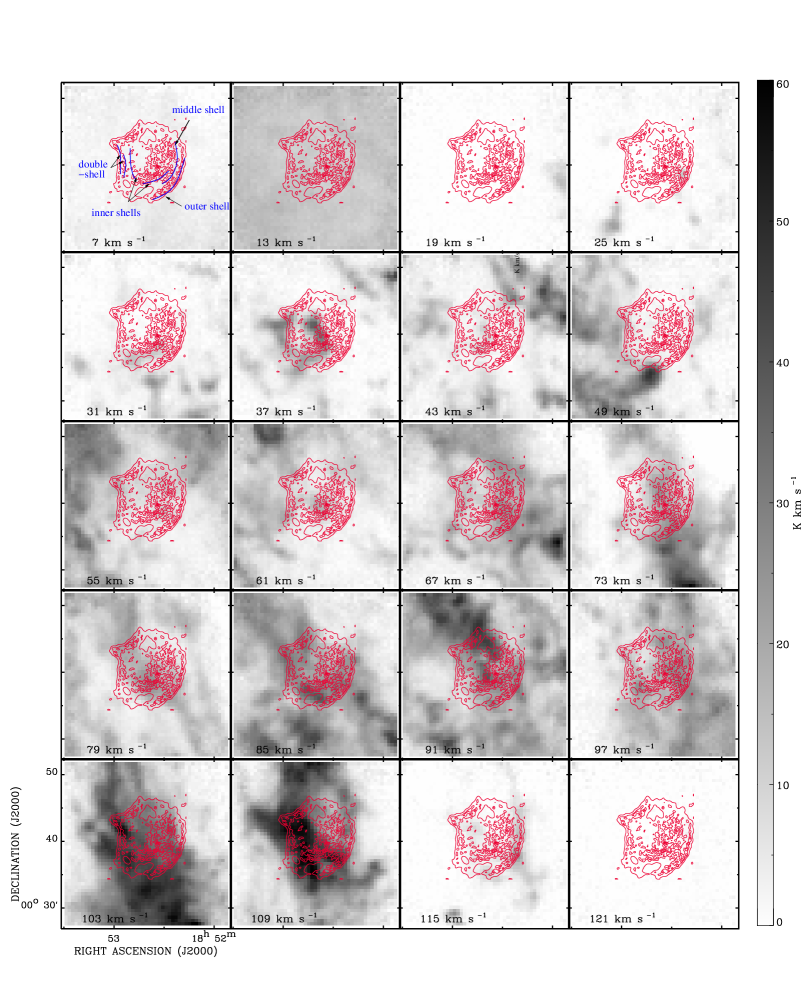
Figure 1.— ¹²CO $J=1$–0 channel maps in the velocity range 4–124 $\,{\rm km}\,{\rm s}^{-1}$, overlaid with contours of the Very Large Array 20 cm continuum emission (Velusamy et al. 1991). The color bar on the right side shows the intensity scale of the channel maps (3$\sigma$–60 $\,{\rm K}$; here $\sigma$ is the root mean square (rms) of the spectrum at each pixel). In the upper-left panel, we define several radio shells which are used for multi-wavelength comparison.

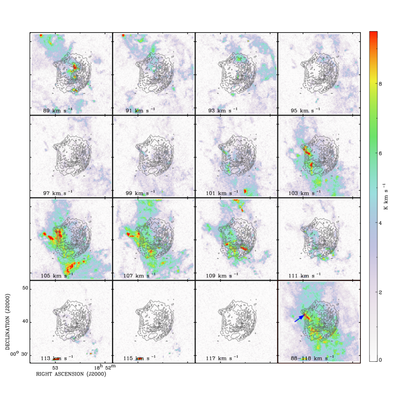
Figure 2.— ¹²CO $J=3$–2 intensity channel maps in the velocity range 99.5–114.5 $\,{\rm km}\,{\rm s}^{-1}$, overlaid with contours of the Very Large Array 20 cm continuum. The color bar on the right side shows the intensity scale of the channel maps (3$\sigma$–9.5 $\,{\rm K}$; here $\sigma$ is the rms of the spectrum at each pixel). The bottom-right panel shows the velocity-integrated intensity. The arrow denotes a clump showing a broad ¹²CO $J=3$–2 line profile (see Figure 3).

Figure 3.— The ¹²CO $J=3$–2 spectrum of the clump at around the radio protrusion (denoted by the arrow in Fig 2) fit with a two-Gaussian model (solid line). The narrow component with $\Delta v\approx 2~{}\,{\rm km}\,{\rm s}^{-1}$ and the broad component with $\Delta v\approx 12~{}\,{\rm km}\,{\rm s}^{-1}$ are shown with dotted line and dashed line, respectively.

Broad molecular line broadening or asymmetric profile is an evidence of shock perturbation of molecular gas (e.g., Denoyer 1979; Chen et al. 2014). A broad ¹²CO $J=3$–2 line is found in the bright clump at the southern boundary of the radio protrusion (${18}^{{\rm h}}{52}^{{\rm m}}{58}^{\rm s}58$, ${00}^{\circ}{42}^{\prime}{29}^{\prime\prime}95$, J2000; with size of $\sim 30^{\prime\prime}$ and denoted by an arrow in Figure 2). As shown in Figure 3, the spectrum consists of a sharp peak at 103 $\,{\rm km}\,{\rm s}^{-1}$ and a broad wing spanning a velocity range over 20 $\,{\rm km}\,{\rm s}^{-1}$, which cannot be explained with a single excitation component. We find that the profile can be well described by two Gaussian components: a narrow line with line width (FWHM) $\Delta v\approx 2$ $\,{\rm km}\,{\rm s}^{-1}$ at $V_{\scriptscriptstyle\rm LSR}\approx 103.3$ $\,{\rm km}\,{\rm s}^{-1}$; and a broad line with $\Delta v\approx 12$ $\,{\rm km}\,{\rm s}^{-1}$ at $V_{\scriptscriptstyle\rm LSR}\approx 104.4$ $\,{\rm km}\,{\rm s}^{-1}$. The narrow line corresponds to the dense, quiescent gas, while the broad component is probably emitted by the shocked gas. The broad ¹²CO $J=3$–2 line detected at the protrusion position, together with the morphological agreement between the two molecular filaments in the east and the radio double shell, supports that the systemic velocity of Kes 79 is at $\sim 105$ $\,{\rm km}\,{\rm s}^{-1}$.

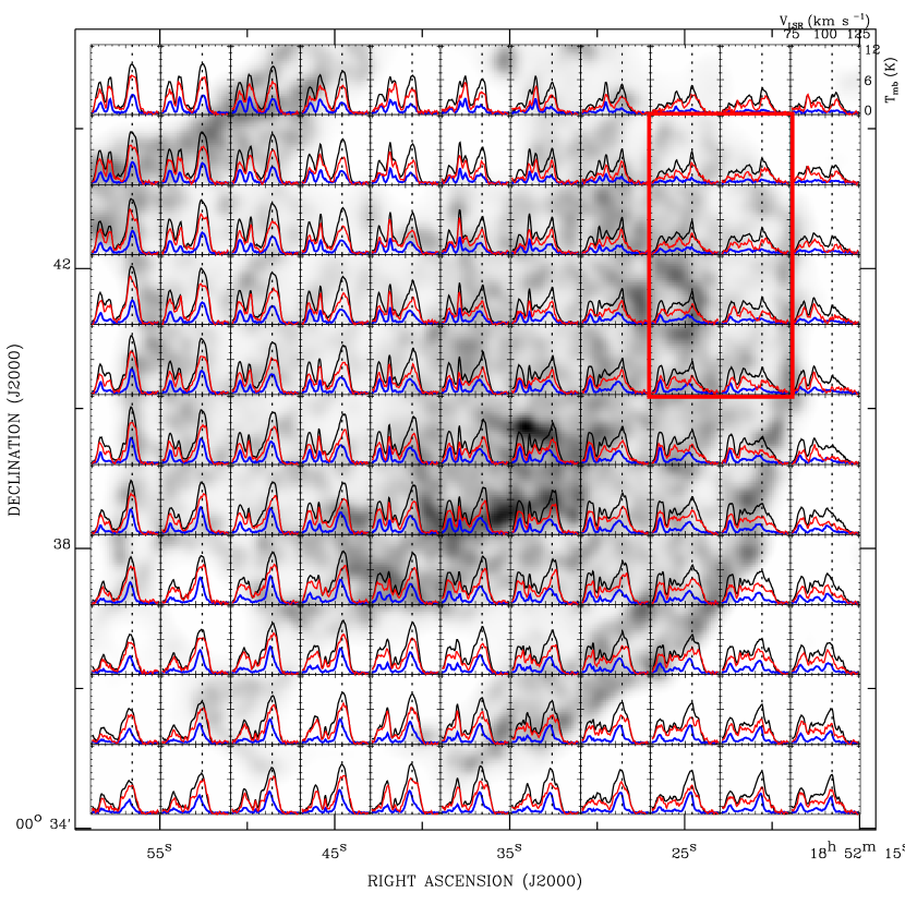
Figure 4.— ¹²CO $J=1$–0 (black), ¹²CO $J=2$–1 (red) and ¹³CO (blue) spectra in the 75–125 $\,{\rm km}\,{\rm s}^{-1}$ velocity range, superposed on the VLA 20 cm image. The scales of $V_{\scriptscriptstyle\rm LSR}$ and $T_{\rm mb}$ are labeled in the upper-right corner. The $J=1$–0 data cubes were convolved with a Gaussian kernel to match the beam size of the ¹²CO $J=2$–1 ($130^{\prime\prime}$). Here the pixel size is $60^{\prime\prime}$. The vertical dashed lines denote the velocity 105 $\,{\rm km}\,{\rm s}^{-1}$. The red rectangle highlights spectra showing strongly asymmetric features extended to $\sim 120~{}\,{\rm km}\,{\rm s}^{-1}$.

We subsequently search for shocked molecular gas over the entire SNR. Figure 4 shows a grid of line profiles of ¹²CO $J=1$–0, ¹³CO $J=1$–0, ¹²CO $J=2$–1 in the 75–125 $\,{\rm km}\,{\rm s}^{-1}$ velocity range across the whole SNR. The radio image is displayed as a background. Due to a low abundance of ¹³CO in the interstellar molecular gas ([¹³CO]/[H${}_{2}]\sim 2\times 10^{-6}$; Dickman 1978), the ¹³CO emission is normally optically thin and traces the quiescent gas. The molecular gas shocked by the SNR may show asymmetric or broad ¹²CO lines deviating from the line profiles of ¹³CO. The ¹³CO emission associated with the SNR peaks at $V_{\scriptscriptstyle\rm LSR}\sim 105~{}\,{\rm km}\,{\rm s}^{-1}$ across the remnant. In the western hemisphere of the remnant, the ¹²CO lines shift to higher velocity (red-shift) relative to the ¹³CO line peaks. The ¹²CO line profiles in the northeast of the remnant (in the red rectangle in Figure 4) show strongly asymmetric features and appear to extend to 120 $\,{\rm km}\,{\rm s}^{-1}$ Figure 5 reveals the distribution intensity weighted mean velocity (first moment; velocity field) of ¹³CO and ¹²CO lines. The ¹²CO emission, especially ¹²CO $J=2$–1, has a higher mean velocity than the systemic velocity given by the ¹³CO emission in the west. Notably, the high-$V_{\scriptscriptstyle\rm LSR}$ ¹²CO emission delineates the outer, middle, and the eastern inner radio shells, suggesting this high-$V_{\scriptscriptstyle\rm LSR}$ emission is excited by the shock at the SNR shells.

3.2. Multi-wavelength Imaging

3.2.1 Filaments Revealed in X-Ray and Other Bands

Figure 5.— Velocity field (first moment) maps of ¹³CO $J=1$–0 (left), ¹²CO $J=1$–0 (middle) and ¹²CO $J=2$–1 (right) in the velocity range 95–115 $\,{\rm km}\,{\rm s}^{-1}$. The $J=1$–0 data cubes were convolved with a Gaussian kernel to match the beam size of the ¹²CO $J=2$–1 ($130^{\prime\prime}$). Here the pixel size is $60^{\prime\prime}$.

We merged the data of the 15 EPIC-MOS observations and show a tri-color image of Kes 79 in Figure 6(a), in which the X-ray emission in the soft (0.3–1.2 keV), medium (1.2–2.0 keV), and hard (2.0–7.0 keV) bands is colored red, green, and blue, respectively. The energy bands are chosen to obtain similar counts in these images. Each of the three band images was exposure-corrected and adaptively smoothed with a Gaussian kernel to achieve a minimum significance of 3 and a maximum significance of 4 using the “csmooth” command in CIAO. The X-ray emission of Kes 79 is highly filamentary and clumpy. In the east, two striking X-ray filaments are distorted and composed of with a string of small X-ray clumps in scale of less than $15^{\prime\prime}$ ($0.5$ pc at a distance of 7.1 kpc). The V-shaped structure in the southern part appears to be the softest X-ray emitter (due to its relatively red color). In the SNR interior, two jet-like filaments stretch from the southeast to the northwest and across the CCO. Near the northwestern end, there is a patch of hard X-ray emission, which is discussed in Section 4.3. The two compact sources, the magnetar 3XMM J185246.6+003317 and the CCO PSR J1852+0040, are located in the south and the center of the SNR, respectively.

The Spitzer $24~{}\,\mu\rm m$ IR image reveals many thin filaments inside the remnant which are well matched with the bright X-ray filaments (see Figure 6b). Here we use the unsharp mask IR image instead of the original emission image in order to highlight the sharp structures.

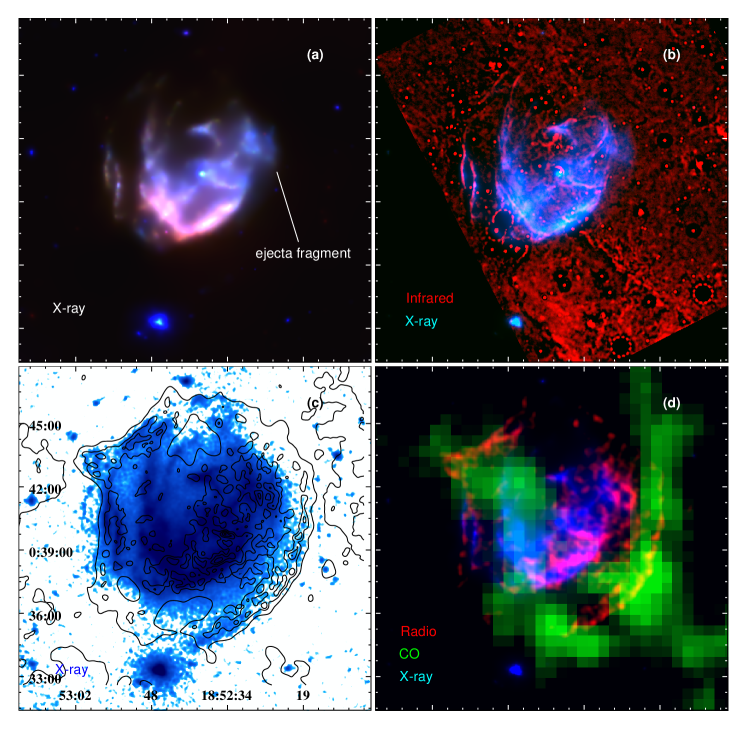
Figure 6.— a) Exposure-corrected and adaptively smoothed EPIC-MOS X-ray image of Kes 79. Red: 0.3-1.2 keV; green: 1.2–2.0 keV; blue: 2.0-7.0 keV. The blue patch in the northwest labeled with “ejecta fragment” is discussed in Section 4.3. b) A composite image of Kes 79 showing the spatial correspondence between the unsharp mask 24 $\mu$m IR image (red) and the 0.3–7.0 keV X-rays (blue). c) 0.3–7.0 keV X-ray image shown on a histogram equalization scale and overlaid with solid, black contours of VLA 20 cm radio continuum emission. d) A tri-color image compares the spatial distribution of the high-$V_{\scriptscriptstyle\rm LSR}$ (110–120 $\,{\rm km}\,{\rm s}^{-1}$) ¹²CO $J=1$–0 emission (green) to those of the radio (red) and 0.3–7.0 keV X-ray emission (blue).

In figure 6d, we compare the distribution of the high-$V_{\scriptscriptstyle\rm LSR}$ MCs (110–120 $\,{\rm km}\,{\rm s}^{-1}$; above the system velocity 105 $\,{\rm km}\,{\rm s}^{-1}$; green) with that of the SNR’s X-ray (blue) and radio (red) emission. A molecular arc delineates the western outer radio shell and confines the bright X-ray emission in the SNR interior. Meanwhile, a northeast-south oriented molecular ridge also spatially matches the bright X-ray filaments and eastern inner radio emission.

3.2.2 X-Ray Halo

A faint X-ray halo surrounding the filamentary structures appears to stretch to the outer radio boundary, as shown in the 0.3–7.0 keV X-ray image (Figure 6(c)). The X-ray image was exposure-corrected, smoothed with a Gaussian kernel of $3\farcm{3}$, and overlaid with contours of the 20 cm radio continuum emission. Here we display the X-ray image with a histogram equalization scale to highlight the faint emission. Unlike the filaments, the faint X-ray halo has no evident IR counterpart. The properties of the X-ray halo and the filaments will be compared in Section 3.3.

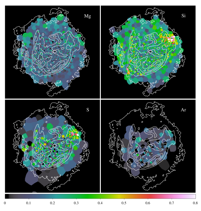
Figure 7.— EW images of He$\alpha$ emission of Mg, Si, S, and Ar overlaid with 0.3–7.0 keV X-ray contours. The contours are made from the X-ray image as shown in Figure 6c and the levels are 1.8, 5.6, 11.2, 19.6, and 28 counts. The band selection is tabulated in Table 2. EWs are set to zero for the bins with S/N$<4$ and low continuum fluxes (4% of the mean flux for the bright line Mg and Si, and 2% of the mean flux for the faint line Si and Ar).

We investigate the distribution of metal lines firstly by using the EW images of Mg He$\alpha$ at $\sim 1.34$ keV, Si He$\alpha$ at $\sim 1.85$ keV, S He$\alpha$ at $\sim 2.45$ keV, and Ar He$\alpha$ at $\sim 3.1$ keV (see Figure 7). The EW of an emission line is defined as $EW=\int I_{\rm l}(E)dE/I_{\rm c}$, where $\int I_{\rm l}(E)dE$ and $I_{\rm c}$ are the energy-integrated intensity of the line component and the intensity of the underlying continuum at the line center, respectively. The EW values of metal lines depend on the abundances, and are also affected by the temperature and ionization states.

We define the energy bands of the lines, and the left and right continuum shoulders as shown in Table 2, according to the global spectra of Kes 79 (see Section 3.3.2 below). The continuum emission of each line is estimated by interpolating the left and right shoulders’ emission. The background of each image is subtracted before producing the EW map. The quiescent particle background (QPB) is first subtracted from each image since it is apparently spatially variant at $\sim 1.49$ keV and $\sim 1.74$ keV, which would affect the EWs of the Mg and Si lines. The QPB images are created from the filter-wheel closed (FWC) data with the XMM-ESAS software. We then estimate the local background level from a region near the remnant and subtract it from the QPB-subtracted image of each band. We adaptively bin the background-subtracted EW images with signal-to-noise ratio (S/N) $\approx 5$ by applying the weighted Voronoi tessellations binning algorithm (Diehl & Statler 2006), which is a generalization of Cappellari & Copin’s (2003) Voronoi binning algorithm. The bins with S/N$<4$ and low continuum fluxes were set to zero.

3.2.3 Equivalent Width (EW) Images of Metal Species

The EWs of the Mg line are nearly uniform across the remnant. Here the Mg He$\alpha$ line’s soft shoulder is strongly affected by the variation of the interstellar absorption, which could also bring uncertainties to the estimation of the continuum.

Asymmetric distribution is clearly revealed in both EW images of Si and S. The largest EW values are found in a patch in the northwest. Generally, the EWs at the X-ray filaments are larger than those in the faint halo regions. A similar trend can also be found in the EW map of Ar. The asymmetric EW distribution of the metal lines suggests that the hot gas properties (abundances, temperature, or ionization states) are not uniform in the SNR. The halo and filamentary regions may not be in the same physical states, as confirmed below according to the spectral analysis.

3.3. XMM-Newton Spectral Analysis

3.3.1 Spectral Extraction and Background Subtraction

The $\gtrsim$ 375 ks XMM-Newton observations allow us to quantitatively investigate the hot gas in small-scale regions in Kes 79. We define source (on-SNR) and background (off-SNR) regions for spectral analysis after removing the central bright X-ray source PSR J1852+0040 by excluding a circular region with a radius of $30^{\prime\prime}$ centered at (${18}^{{\rm h}}{52}^{{\rm m}}{38}^{\rm s}522$, ${00}^{\circ}{40}^{\prime}{20}^{\prime\prime}89$, J2000) (see Figure 8). We select a large region with a radius of $5\farcm{5}$ that covers the whole SNR, 14 small regions for the bright filamentary structures (“f1–14”) and 5 smaller regions (“c”, “mE”, “mW”, “oW”, and “oN”) for the faint halo gas. The background region “bg” is selected from the nearby sky with the same Galactic latitude as that of the remnant to minimize contamination by the Galactic ridge emission.

Table 2Energy ranges selected for the EW maps

Metal Line	Left Shoulder	Line	Right Shoulder
	(keV)	(keV)	(keV)
Mg He$\alpha$	1.16–1.22	1.25–1.42	1.45–1.51
Si He$\alpha$	1.45–1.51	1.75–1.95	1.96–2.08
S He$\alpha$	1.96–2.08	2.30–2.60	2.63–2.78
Ar He$\alpha$	2.63–2.78	2.98–3.22	3.28–3.70

We apply a double-subtraction method that takes into account vignetting effects and the spatially variable instrumental background as follows: (1) subtract respective instrumental background contribution from the raw on- and off-SNR spectra by using the FWC data of MOS1; (2) construct a background model by fitting the off-SNR spectra (instrumental background-subtracted), which is subsequently normalized by area and added to the source model to describe the on-SNR spectra. FWC data are selected in the epochs close to those of the source observations in order to reduce variation of instrumental background. Using the task $addascaspec$ in HEASOFT, we merged the spectra taken within two months to increase the statistical quality for the hard X-ray band. Hence, the spectra of the two 2004 observations, five 2008 observations, and six 2009 observations are merged respectively. Finally, the 10 source spectra (5 MOS1 plus 5 MOS2 spectra taken from the 2004, 2006, 2007, 2008, and 2009 observations) for each on-SNR region are then instrumental background-subtracted and binned to reach an S/N of $>4$ in the following joint-fit. We only use the six off-SNR spectra (region “bg”; 3 MOS1 plus 3 MOS2) taken in 2004, 2006 and 2008 to construct the background model, since the region “bg” was at the unusable CCD of MOS1 during the observations in 2007 and 2009.

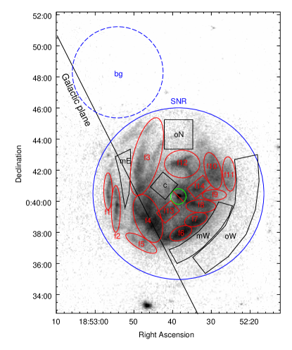
Figure 8.— EPIC-MOS raw image of Kes 79 smoothed with a Gaussian kernel of 3. The solid regions colored in blue, red, and black are defined for spectral extraction of the whole SNR, the filaments, and diffuse gas, respectively. The dashed circle labeled “bg” is selected as the background region. The point sources removed in the concerned area are denoted by the green region with a red slash.

XSPEC (version 12.9) is used for spectral fitting. The spectra in the off-SNR region “bg” is phenomenologically described with an absorbed $nei$+$power$-$law$ plus an unabsorbed $bremsstrahlung$ + $gaussian$ model ($\chi_{\nu}^{2}/d.o.f=1.33/231$; see Figure 9). The on-SNR sky background is determined by normalizing the model according to the region sizes.

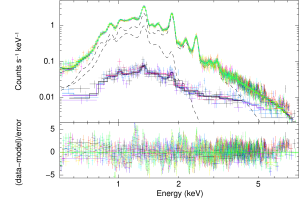
Figure 9.— EPIC-MOS spectra of the whole SNR (upper; 10 groups) and region “bg” (bottom; 6 groups). The source spectra are fitted with an absorbed $nei$ +$vnei$ model (dashed lines) plus the background model (dotted lines; phenomenologically describing the “bg” spectra; note that the area response is different at the the on-SNR and off-SNR regions). The spectral fitting results are summarized in Table 3.

3.3.2 The Global Spectra

Figure 9 shows the spectra extracted from source region “SNR” (upper) and background region “bg” (bottom; normalized by area). The global spectra of the SNR in 0.5–8 keV reveals distinct He-like lines of Mg ($\sim 1.34$ keV), Si ($\sim 1.85$ keV and $\sim 2.19$ keV), S ($\sim 2.45$ keV), and Ar ($\sim 3.1$ keV), and several faint H-like lines of Ne at 0.9 keV and S at 2.9 keV.

We first applied an absorbed non-equilibrium ionization (NEI) model (plus the background model with fixed values) to jointly fit the 10 source spectra in 0.5-8.0 keV. For the foreground absorption, we used the $tbabs$ model with the Anders & Grevesse (1989) abundances and photoelectric cross-section from Balucinska-Church & McCammon (1992). The NEI model $vnei$ (NEI version 3.0 in XSPEC) is firstly applied, with the abundances of Ne, Mg, Si, S, Ar, and Fe (the abundance of Ni is tied to Fe) in the models allowed to vary in the spectral fit. Here $vnei$ describes an NEI plasma with single and uniform ionization parameters. However, the single NEI model fails to describe the spectra in the hard X-ray band ($\chi_{\nu}^{2}/d.o.f=2.98/2657$) as also pointed out by A14. The elevated tail of the observed spectra compared to the model above 3 keV is also seen in single thermal model spectral fittings in previous studies (e.g. S04, and Giacani et al. 2009), implying that the global spectrum of Kes 79 should contain more than one component.

Since some thermal composite SNRs show recombining plasma, we tried an absorbed recombining plasma model ($vrnei$ in XSPEC) to fit the spectra. However, the spectral fit ($\chi_{\nu}^{2}/d.o.f=2.96/2656$) gives an initial plasma temperature (0.12 keV) much smaller than the current plasma temperature (0.75 keV), suggesting that the gas is under-ionized rather than over-ionized.

An absorbed $nei$+$vnei$ model is subsequently used, which substantially improves the spectral fit ($\chi_{\nu}^{2}/d.o.f=1.92/2654$; see Table 3 for the spectral fit results and Figure 9 for the spectra). The abundance of the cool component is set to solar since variable abundance does not apparently improve the spectral fit. The model is still not good enough to reproduce the spectra, especially in the 1-3 keV band, which suggests that the physical properties of the X-ray emitting gas are not uniform across the remnant. However, the two-temperature model, to some extent, provides us with general properties of the hot plasma.

Table 3Spectral Fitting results with the $nei$/$apec$+$vnei$ model

Region	$\chi_{\nu}^{2}$/dof	$N_{\scriptscriptstyle\rm H}$	$kT_{\rm c}$	$\tau_{\rm c}$	$kT_{\rm h}$	$\tau_{\rm h}$	Ne	Mg	Si	S	Ar	Fe	$n_{\rm c}$	$n_{\rm h}$	$t_{i,{\rm h}}$
		($10^{22}\,{\rm cm}^{-2}$)	(keV)	($10^{11}\,{\rm cm}^{-3}$ s)	(keV)	($10^{10}\,{\rm cm}^{-3}$ s)							($\,{\rm cm}^{-3}$)	($\,{\rm cm}^{-3}$)	(kyr)
SNR	1.92 /2654	1.707${}_{-0.099}^{+0.004}$	0.195${}_{-0.002}^{+0.003}$	6.4$\pm 0.4$	0.80$\pm 0.01$	8.1$\pm 0.1$	1.83${}_{-0.05}^{+0.04}$	1.56$\pm 0.03$	1.40$\pm 0.02$	1.72$\pm 0.03$	1.8$\pm 0.1$	0.93$\pm 0.04$	2.1	0.5	4.2
f1	1.01 / 501	1.8$\pm 0.1$	0.21${}_{-0.01}^{+0.03}$	6.4 ($>2.7$)	0.7${}_{-0.1}^{+0.2}$	6.6${}_{-2.3}^{+4.2}$	2.0${}_{-0.7}^{+1.3}$	1.8${}_{-0.4}^{+0.7}$	1.5$\pm 0.3$	1.8${}_{-0.4}^{+0.7}$	1 (fixed)	1.5${}_{-0.5}^{+0.9}$	5.7	1.7	1.0
f2	1.06 / 697	1.77$\pm 0.09$	0.19${}_{-0.02}^{+0.02}$	6.7 ($>2.6$)	0.73${}_{-0.07}^{+0.09}$	7.7${}_{-2.0}^{+2.7}$	2.5${}_{-0.7}^{+0.9}$	1.6$\pm 0.3$	1.6${}_{-0.2}^{+0.3}$	2.1$\pm 0.3$	1 (fixed)	1.2${}_{-0.4}^{+0.5}$	6.0	1.6	1.3
f3	1.19 /1249	1.84$\pm 0.05$	0.20$\pm 0.01$	6.2${}_{-2.2}^{+3.4}$	0.75$\pm 0.04$	7.6${}_{-1.1}^{+1.2}$	2.2$\pm 0.03$	1.6$\pm 0.02$	1.6${}_{-0.1}^{+0.2}$	1.9$\pm 0.2$	2.8$\pm 0.8$	1.1${}_{-0.2}^{+0.3}$	3.8	1.0	2.0
f4	1.28 /1622	1.63${}_{-0.04}^{+0.02}$	0.197${}_{-0.004}^{+0.003}$	5.4${}_{-0.8}^{+2.7}$	0.91${}_{-0.02}^{+0.03}$	6.4${}_{-0.6}^{+0.3}$	2.5$\pm 0.2$	1.8$\pm 0.1$	1.48${}_{-0.08}^{+0.03}$	1.82${}_{-0.10}^{+0.07}$	1.5$\pm 0.3$	0.94${}_{-0.13}^{+0.07}$	8.1	1.8	1.0
f5	0.97 / 614	1.6$\pm 0.1$	0.19$\pm 0.01$	7.5 ($>2.9$)	1.4${}_{-0.2}^{+0.3}$	2.3${}_{-0.4}^{+0.5}$	2.8${}_{-0.9}^{+1.1}$	1.9${}_{-0.4}^{+0.5}$	1.7${}_{-0.3}^{+0.4}$	1.8${}_{-0.3}^{+0.4}$	1 (fixed)	1.1${}_{-0.5}^{+0.6}$	6.2	0.8	0.8
f6	1.18 /1093	1.58$\pm 0.05$	0.200${}_{-0.003}^{+0.008}$	7.2${}_{-2.0}^{+7.5}$	0.82${}_{-0.05}^{+0.06}$	9.6${}_{-1.5}^{+1.6}$	2.6$\pm 0.5$	1.9$\pm 0.2$	1.7${}_{-0.2}^{+0.1}$	2.0$\pm 0.2$	1.6$\pm 0.5$	1.0$\pm 0.2$	13.0	3.2	0.8
f7	1.14 /1075	1.68${}_{-0.05}^{+0.07}$	0.20$\pm 0.01$	13.4 ($>6.5$)	0.91${}_{-0.04}^{+0.05}$	7.2${}_{-1.3}^{+0.9}$	2.3${}_{-0.5}^{+0.6}$	1.8$\pm 0.2$	1.5$\pm 0.2$	1.8$\pm 0.2$	1.1$\pm 0.5$	0.9$\pm 0.2$	13.2	2.8	0.7
f8	1.20 /1060	1.81${}_{-0.04}^{+0.03}$	0.21${}_{-0.02}^{+0.01}$	…	0.91$\pm 0.03$	6.8${}_{-0.8}^{+1.1}$	2.1${}_{-0.3}^{+0.4}$	2.0$\pm 0.2$	1.6$\pm 0.2$	1.9$\pm 0.2$	1.3${}_{-0.5}^{+0.6}$	1.1${}_{-0.2}^{+0.3}$	8.8	2.2	0.9
f9	1.07 / 620	1.9$\pm 0.1$	0.21$\pm 0.03$	7.0 ($>3.5$ )	0.9$\pm 0.1$	6.7${}_{-1.5}^{+3.1}$	2.0${}_{-0.7}^{+1.1}$	2.2$\pm 0.5$	1.7${}_{-0.3}^{+0.4}$	1.9${}_{-0.4}^{+0.5}$	2.6${}_{-1.2}^{+1.4}$	1.5${}_{-0.5}^{+0.7}$	7.6	1.8	1.0
f10	1.17 /1064	1.90$\pm 0.03$	0.22$\pm 0.01$	…	1.18${}_{-0.06}^{+0.07}$	2.4$\pm 0.2$	2.8${}_{-0.5}^{+0.6}$	2.8${}_{-0.3}^{+0.4}$	3.1$\pm 0.3$	3.4$\pm 0.4$	3.6${}_{-1.1}^{+1.2}$	1.0$\pm 0.3$	6.6	1.2	0.5
f11	1.03 / 629	2.0$\pm 0.1$	0.19$\pm 0.01$	5.9${}_{-2.7}^{+9.8}$	1.6${}_{-0.3}^{+0.6}$	3.2${}_{-0.7}^{+0.8}$	4.4${}_{-2.2}^{+3.5}$	3.6${}_{-1.0}^{+1.7}$	5.2${}_{-1.3}^{+2.2}$	5.2${}_{-1.1}^{+1.8}$	4.2${}_{-1.8}^{+2.4}$	0.6${}_{-0.6}^{+1.6}$	7.9	1.0	0.9
f12	1.11 /1066	1.82${}_{-0.06}^{+0.05}$	0.20${}_{-0.01}^{+0.02}$	7.5${}_{-3.4}^{+20.3}$	0.74${}_{-0.04}^{+0.05}$	9.9${}_{-1.8}^{+2.0}$	1.8$\pm 0.4$	1.7$\pm 0.2$	1.4$\pm 0.2$	1.8$\pm 0.2$	1.2${}_{-0.6}^{+0.7}$	1.1${}_{-0.2}^{+0.3}$	6.0	1.7	1.6
f13	1.07 / 998	1.66$\pm 0.04$	0.18$\pm 0.01$	…	0.89${}_{-0.06}^{+0.05}$	10.0${}_{-2.0}^{+1.9}$	2.1$\pm 0.3$	1.9$\pm 0.2$	1.5${}_{-0.1}^{+0.2}$	1.6$\pm 0.2$	1.7$\pm 0.5$	1.0${}_{-0.2}^{+0.3}$	12.4	2.5	1.0
f14	1.10 / 924	1.83${}_{-0.04}^{+0.03}$	0.22$\pm 0.01$	…	0.88${}_{-0.10}^{+0.07}$	7.2${}_{-1.1}^{+2.2}$	2.3$\pm 0.5$	1.9${}_{-0.2}^{+0.3}$	1.6${}_{-0.2}^{+0.1}$	1.8${}_{-0.2}^{+0.3}$	1.2${}_{-0.6}^{+0.7}$	0.7$\pm 0.3$	9.1	2.2	0.9
c	0.98 / 723	1.9$\pm 0.1$	0.19$\pm 0.01$	4.8${}_{-2.4}^{+5.7}$	0.9$\pm 0.1$	7.8${}_{-1.6}^{+2.3}$	3.0${}_{-0.8}^{+1.5}$	1.5$\pm 0.3$	1.3${}_{-0.2}^{+0.3}$	1.6${}_{-0.2}^{+0.3}$	0.9${}_{-0.7}^{+0.8}$	0.5${}_{-0.5}^{+0.4}$	2.4	0.5	4.1
mE	1.15 / 351	1.62${}_{-0.08}^{+0.11}$	0.17$\pm 0.05$	…	0.7${}_{-0.1}^{+0.3}$	7.2${}_{-4.5}^{+10.4}$	0.9${}_{-0.6}^{+0.9}$	1.2${}_{-0.3}^{+0.5}$	1.1${}_{-0.2}^{+0.4}$	1.3${}_{-0.4}^{+0.5}$	1 (fixed)	1.1${}_{-0.4}^{+0.7}$	1.4	0.3	6.3
mW	1.15 / 836	1.66${}_{-0.08}^{+0.06}$	0.20${}_{-0.01}^{+0.02}$	7.8 ($>4.4$)	1.0${}_{-0.1}^{+0.2}$	5.4${}_{-1.6}^{+1.9}$	2.3${}_{-0.6}^{+1.1}$	1.8${}_{-0.3}^{+0.4}$	1.5${}_{-0.2}^{+0.3}$	1.7${}_{-0.3}^{+0.4}$	1.6${}_{-1.1}^{+1.2}$	1.1$\pm 0.4$	2.1	0.4	3.5
oW	1.07 / 804	1.72$\pm 0.08$	0.18${}_{-0.01}^{+0.02}$	2.1${}_{-1.2}^{+3.8}$	0.68${}_{-0.06}^{+0.09}$	12.4${}_{-5.1}^{+10.8}$	1.3${}_{-0.4}^{+0.6}$	1.4${}_{-0.2}^{+0.4}$	1.2${}_{-0.2}^{+0.4}$	1.5${}_{-0.3}^{+0.5}$	1 (fixed)	1.7${}_{-0.5}^{+0.7}$	1.2	0.3	10.9
oN	1.15 / 406	1.7$\pm 0.1$	0.19${}_{-0.03}^{+0.04}$	4.5 ($>1.1$)	0.7${}_{-0.1}^{+0.2}$	7.6${}_{-3.3}^{+8.4}$	1.9${}_{-0.8}^{+1.6}$	1.8${}_{-0.5}^{+1.0}$	1.5${}_{-0.4}^{+0.8}$	1.7${}_{-0.6}^{+1.0}$	1 (fixed)	1.3${}_{-0.7}^{+1.1}$	1.8	0.5	4.0

Note. — The errors are estimated at the 90% confidence level.

According to the $nei$+$vnei$ model, the X-rays from the remnant suffers an interstellar absorption $N_{\scriptscriptstyle\rm H}=1.71\times 10^{22}\,{\rm cm}^{-2}$ and the X-ray-emitting plasma can be roughly described as under-ionized two-temperature gas. The cool phase of the gas has a temperature $kT_{\rm c}=0.19$ keV, an ionization timescale $\tau_{\rm c}=n_{e,{\rm c}}t_{i,{\rm c}}=6.4\pm 0.4\times 10^{11}~{}\,{\rm cm}^{-3}\,{\rm s}$ , and solar abundances (so fixed to 1), while the hot phase has a temperature $kT_{\rm h}=0.80$ keV, an ionization timescale $\tau_{\rm h}=n_{e,{\rm h}}t_{i,{\rm h}}=8.1\pm 0.1\times 10^{10}~{}\,{\rm cm}^{-3}\,{\rm s}$ and enriched metal abundances ([Ne]/[Ne]${}_{\odot}=1.83\pm 0.05$, [Mg]/[Mg]${}_{\odot}=1.56\pm 0.03$, [S]/[S]${}_{\odot}=1.40\pm 0.02$, and [Ar]/[Ar]${}_{\odot}=1.8\pm 0.1$).

The column density (inferred from the $tbabs$ model) is larger than that obtained by S04 ($1.54\pm 0.5\times 10^{22}~{}\,{\rm cm}^{-2}$, $phabs$ model) and Giacani et al. (2009; $1.52\pm 0.02\times 10^{22}~{}\,{\rm cm}^{-2}$, $phabs$ model), but smaller than that reported by A14 ($2.43\pm 0.05\times 10^{22}~{}\,{\rm cm}^{-2}$; $tbabs$ model). Some other spectral fit results, such as $kT_{\rm c}$ and abundances, are also different from those obtained by A14. We believe that the background selection is the main reason for the discrepancy between our work and A14. In particular, some of the background regions selected by A14 are well inside the SNR where halo X-ray emission is present (see Figure 6c in this paper in comparison to Figure 3 in A14).

We assume that the two-temperature gas fills the whole volume ($f_{\rm c}+f_{\rm h}=1$) and is in pressure balance ($n_{\rm c}T_{\rm c}=n_{\rm h}T_{\rm h}$), where $f$ and $n$ are the filling factor and hydrogen density ($n=1.2n_{e}$), respectively. The subscripts “c” and “h” denote the parameters for the cool and hot phases, respectively. The $nei$+$vnei$ fit results (see Table 3) give an emission measure $f_{\rm c}n_{e,{\rm c}}n_{\rm c}Vd_{7.1}^{-2}=5.9^{+0.3}_{-0.2}\times 10^{59}~{}\,{\rm cm}^{-3}$ for the cool phase gas, and $f_{\rm h}n_{e,{\rm h}}n_{\rm h}Vd_{7.1}^{-2}=2.2\pm 0.1\times 10^{58}~{}\,{\rm cm}^{-3}$ for the hot phase, where $V$ is the volume of the sphere and $d_{7.1}$ is the distance scaled to 7.1 kpc. The cool component is found to fill 62% of the volume, with a larger density $n_{\rm c}=2.1^{+0.5}_{-0.3}(f_{\rm c}/0.62)^{-1/2}d_{7.1}^{-1/2}~{}\,{\rm cm}^{-3}$, while the hot component has a density $n_{\rm h}=0.51^{+0.02}_{-0.01}(f_{\rm h}/0.38)^{-1/2}d_{7.1}^{-1/2}~{}\,{\rm cm}^{-3}$. Then we can obtain the ionization age for the two components $t_{c}=\tau_{\rm c}/n_{\rm e,c}\sim 8.1$ kyr and $t_{h}=\tau_{\rm h}/n_{\rm e,h}\sim 4.2$ kyr. The larger ionization age of the cool phase is possibly due to a variable $n_{\rm e,c}$ (e.g., decreasing with time).

3.3.3 Spatially resolved spectroscopy

The X-ray image of Kes 79 (see Figure 6a) has revealed a non-uniform nature of the hot gas. The EW maps of metal lines (Figure 7) also indicate a nonuniform distribution of the ejecta. The gas properties are thus expected to be spatially variant, and the global spectra may not be well described with a simple one-component or two-component model. We thus compare the spectral analysis results of the 19 defined small regions to investigate the variation of gas properties across the SNR.

A two-component thermal model is needed to describe the spectra well for the 19 small-scale regions. Adding an extra model to a single thermal model is also feasible according to the F-test null hypothesis probabilities. We first use $nei$(soft)+ $vnei$(hard) to fit the spectra, and then replace $nei$ with $apec$ (APEC thermal model describing the plasma in collisional ionization equilibrium; ATOMDB version 3.0.2) for the cool phase if its ionization timescale reaches higher than $\sim 10^{13}~{}\,{\rm cm}^{-3}\,{\rm s}$. Here we allow the Ne, Mg, Si, S, Ar, and Fe abundances of the hot component to vary as long as they can be well constrained. The abundance of the cool component is set to solar since variable abundance does not apparently improve the spectral fit. The best-fit results for the $nei$/$apec$+$vnei$ model are tabulated in Table 3.

The interstellar column density $N_{\scriptscriptstyle\rm H}$ of the X-ray emission varies from $\sim 1.5\times 10^{22}\,{\rm cm}^{-2}$ in the south to $\sim 2.0\times 10^{22}\,{\rm cm}^{-2}$ in the northwest, consistent with the fact that the southern portion emits softer X-rays (as shown in Figure 6a). Generally, both the bright filamentary (except regions “f5”, “f10” and “f11”) and faint halo gas hold spectral properties similar to the global SNR gas, including the temperature of the cool phase ($kT_{\rm c}\sim 0.2$ keV), and the temperature ($kT_{\rm h}\sim 0.7$–1.0 keV), ionization timescale ($\tau_{\rm h}=6$–$12\times 10^{10}~{}\,{\rm cm}^{-3}\,{\rm s}$), and metal abundances of the hot phase. Nevertheless, there is a trend that the gas near the SNR edge has lower $kT_{\rm h}$ ($\sim 0.7$ keV) than in the SNR center ($\sim 0.9$ keV).

To estimate the density of the plasma, we assume several three-dimensional shapes for the two-dimensional regions: (1) oblate spheroids for the elliptical regions “f1–12”; (2) oblate cylinders for the rectangular regions “f13–14”; (3) sections of spherical layers for the shell-like halo regions “mW” and “oW”; 4) for the halo regions “c”, “mE” and “oN”, the volumes are expressed as $V=S\times l$; where $S$ is the area of the region and $l$ is the line of sight length along the SNR sphere (depending on the distance of the region to the SNR center). We assume that $f_{\rm c}+f_{\rm h}=1$ and $n_{\rm c}T_{\rm c}=n_{\rm h}T_{\rm h}$, similar to the calculation for the global gas. The calculated densities of the two-phase gas are summarized in Table 3.

4. Discussion

4.1. Multi-wavelength Manifestation of the SNR-MC Interaction

4.1.1 Molecular environment

Using the multi-transition CO observations, we have provided kinematic and new morphological evidence to support the scenario that Kes 79 is interacting with MCs at a systemic LSR velocity of $\sim 105~{}\,{\rm km}\,{\rm s}^{-1}$.

The column density and mass of the surrounding molecular gas can be estimated by using the ¹³CO $J=1$–0 lines spanning the velocity range of 95–115 $\,{\rm km}\,{\rm s}^{-1}$. Assuming that the rotational levels of the ¹³CO molecules are in local thermodynamic equilibrium, we obtain the column density of ¹³CO molecules as follows (Kawamura et al. 1998):

$$N(^{13}{\rm CO})=2.42\times 10^{14}~{}\frac{\tau(^{13}{\rm CO})\Delta v(\,{\rm km}\,{\rm s}^{-1})T_{\rm ex}(\,{\rm K})}{1-\exp(-5.29\,{\rm K}/T_{\rm ex})}~{}\,{\rm cm}^{-2},$$ (1)

where $T_{\rm ex}$ and $\Delta v$ are the excitation temperature and line width of ¹³CO $J=1$–0, respectively. When the ¹³CO lines are optically thin (optical depth $\tau(^{13}{\rm CO})\ll$ 1), the main beam brightness temperature of ¹³CO is $T_{\rm mb}\approx T_{\rm ex}\tau(^{13}{\rm CO})$. Considering that $T_{\rm mb}\Delta v\approx\int T_{\rm mb}(v)dv$ and taking the $N({\rm H}_{2})$ to $N(^{13}{\rm CO})$ ratio as $5\times 10^{5}$ (Dickman 1978), we obtain the column density of H₂:

$$N({\rm H}_{2})=1.21\times 10^{20}\frac{\int T_{\rm mb}(v)dv(\,{\rm K})}{1-\exp(-5.29/T_{\rm ex})}~{}\,{\rm cm}^{-2}.$$ (2)

A typical MCs temperature of 10 K is adopted here for $T_{\rm ex}$, which is also close to the peak main beam temperature of ¹²CO $J=1$–0 lines in the vicinity of Kes 79 (see Figure 4). The ¹³CO emission integrated in the velocity range 95–115 $\,{\rm km}\,{\rm s}^{-1}$ (associated with the SNR) is then used to derive the $N({\rm H}_{2})$ and the distribution of $N({\rm H}_{2})$ near the remnant is revealed in Figure 10.

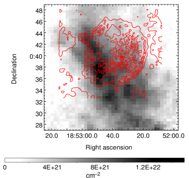
Figure 10.— Distribution of the H₂ column density (estimated from ¹³CO $J=1$–0 in the velocity range 95–115 $\,{\rm km}\,{\rm s}^{-1}$) in the vicinity of Kes 79, VLA 20 cm radio contours are overlaid.

The mass of the environmental molecular gas in the $22^{\prime}\times 22^{\prime}$ (or $45.4d_{7.1}$ pc $\times 45.4d_{7.1}$ pc) region (field of view in Figure 10), is obtained to be $M_{\rm mol}=\mu m_{\rm H}\sum[N({\rm H}_{2})L^{2}]\sim 5.7d_{7.1}^{2}\times 10^{4}~{}M_{\odot}$, where the mean molecular weight $\mu=2.8$, $m_{\rm H}$ is the mass of the hydrogen atom, and $L$ is the size of the gas ($45.4d_{7.1}$ pc). The size and mass values of the cloud is typical for giant MCs (GMCs; Dame et al. 2001). The mean molecular density of the GMC can be estimated as $n({\rm H}_{2})\sim{\overline{N}({\rm H}_{2})}/L\sim 30d_{7.1}^{-1}~{}\,{\rm cm}^{-3}$, where ${\overline{N}({\rm H}_{2})}$ is the mean column density.

4.1.2 Origin of the Mid-IR and X-Ray Filaments

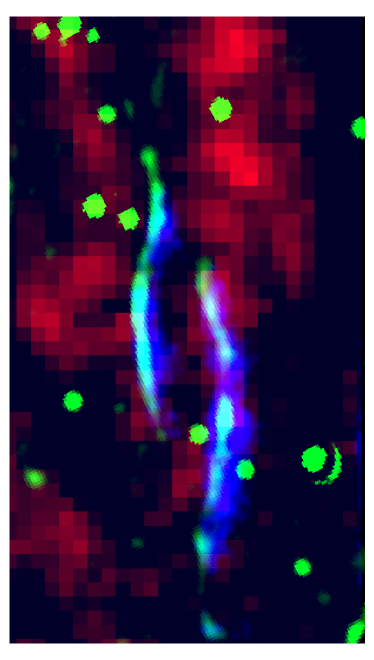
Figure 11.— Tri-color image of the twin filaments in the east of Kes 79. Red: JCMT ¹²CO $J=3$–2 image at 105 $\,{\rm km}\,{\rm s}^{-1}$; green: unsharp mask Spitzer 24 $\,\mu\rm m$ image; blue: XMM-Newton MOS 0.3–7.0 keV.

A good spatial correlation is present between the mid-IR filaments and the X-ray filaments (see Figure 6). Previous IR studies toward middle-age SNRs summarized three main origins of the emission at the Spitzer 24 $\,\mu\rm m$ band: (1) continuum emission of dust grains (e.g., Andersen et al. 2011); (2) atomic lines such as [Fe II] at 25.988 $\,\mu\rm m$ and [O IV] at 25.890 $\,\mu\rm m$ (e.g., Reach & Rho 2000), and (3) molecular lines such as the vibrational rotational line of H₂ at 28.2 $\,\mu\rm m$ (e.g., Neufeld et al. 2007). The IR emission at $\gtrsim 15$ $\,\mu\rm m$ is usually dominated by the continuum of dust grains with typical temperature $\sim 40$–100 K (Seok et al. 2013), while at the shorter wavelengths, the IR emission of SNRs can be dominated by ionic/molecular lines (e.g., IC 443, Cesarsky et al. 1999; 3C 391, Reach et al. 2002). The warm dust could be heated by either collisions or radiation. In the collisions case, the swept-up dust grains are collisionally heated by the electrons in the hot plasma (Dwek 1987), which results in a good spatial correlation between the IR and X-ray emission. The dust grains could also be heated by the UV photons from the postshock gas in the radiative shock (Hollenbach & McKee 1979), which may be efficient for the SNRs interacting with MCs. Considering the MC–IR-X–ray correlation revealed in Kes 79 (Figure 6), the two cases may both work here. The SNR has been considered to be in the Sedov phase of evolution (S04; see also discussion in Section 4.2) and no optical emission has been detected to support the radiative shock scenario (could possibly be due to heavy absorption). However, small-scale radiative shock in MCs cannot be excluded. Since the IR emission is filamentary and a strong IR-X-ray correlation is widely seen in the whole remnant (see Figure 6b), it is more likely that the $24~{}\,\mu\rm m$ emission comes from dust heated by the hot plasma. Further IR spectroscopic observations are required to provide a firm conclusion.

The most prominent IR filaments emerge in the eastern section of the SNR, where there is good correlation with the X-ray structures, including the enhancements at several clumps. In Figure 11, we show the two filaments in the eastern part of the SNR revealed in ¹²CO $J=3$–2, 24 $\,\mu\rm m$, and the 0.3–7.0 keV X-ray bands. The three bands correspond to three hierachical gas phases: cold dense gas, warm gas/dust, and hot tenuous plasma. There is a trend wherein the colder gas is located east of the hotter gas. In particular, the thin IR filaments with a width of $6^{\prime\prime}$ (0.2 pc at a distance of 7.1 kpc) are just east of the X-ray filaments ($\sim 15^{\prime\prime}$). The trend is consistent with a scenario where the shock is interacting with multi-phase ISM in the east, which then generates different types of shocks. The shock is damped while it propagates into denser medium. The fast shocks heat the moderate-density cloudlet ($n_{\rm c}\sim 6~{}\,{\rm cm}^{-3}$) to a temperature of $kT_{\rm c}\sim 0.2$ keV and the low-density inter-cloud medium ($n_{\rm h}\sim 1$–$2~{}\,{\rm cm}^{-3}$) to a temperature of $kT_{\rm h}\sim 0.7$ keV (see Table 3). The nondissociative shock transmitted into the dense molecular clumps ($>10^{4}\,{\rm cm}^{-3}$ for the clumps emitting ¹²CO $J=3$–2 emission) has a low velocity ($\lesssim 50\,{\rm km}\,{\rm s}^{-1}$, Draine & Mckee 1993) and generates the broad/asymmetric ¹²CO lines. Therefore, the multiple shocks in clumpy ISM explains the bright filamentary radiation in multi-wavelengths.

The interior X-ray filaments probably arise from SNR interaction with relatively dense gas ($\sim 4$–$13~{}\,{\rm cm}^{-3}$ for the cold component), as compared to the low density of the halo gas ($\sim 1$–$2~{}\,{\rm cm}^{-3}$ for the cold component; see Table 3).

4.1.3 Projection Effects

Kes 79 was classified as a mixed-morphology or thermal composite SNR (Rho & Petre 1998), as its brightest X-ray emission arises from the interior and the radio emission is shell-like, Different from most other thermal composite-type SNRs, which have a smooth, centrally filled X-ray morphology, Kes 79 has a highly structured X-ray morphology, and the interior X-ray and radio emission are correlated (see Figure 6). As S04 note, the inner X-ray shell and outer X-ray halo have clear-cut edges and may both come from shock surfaces. In Section 4.1.2, we have provided evidence that the X-ray and IR filaments, and the radio shells in the SNR interior result from the interaction of the shock with a dense medium. Hence, projection effect is the most plausible origin of the multiple-shell structure mixed-morphology nature.

Kes 79 may have a double-hemisphere morphology viewed essentially along the symmetric axis. SNRs breaking out from an MC into a low-density region can produce such a double-hemisphere morphology as predicted by hydrodynamic simulations (e.g., Tenorio-Tagle et al. 1985; Cho et al. 2015). There are a number of SNRs showing such double-hemisphere morphology due to shock breaking out from a dense medium, such as IC 443 (e.g., Troja et al. 2006), W28 (e.g., Dubner et al. 2000), 3C391 (e.g., Reynolds & Moffett 1993, Chen et al. 2004), VRO 42.05.01 (e.g., Pineault et al. 1987), G349.7$+0.2$ (e.g., Lazendic et al. 2005), etc. All of these SNRs are associated with MCs (see Jiang et al. 2010 and references therein). Here we suggest that Kes 79 is among the group of double-hemisphere SNRs interacting with MCs. The bright filaments correspond to the smaller hemisphere (radius $R_{1}\sim 4^{\prime}$) evolving into the denser ISM, while the shock breaking out in a tenuous medium forms a larger hemisphere (radius $R_{2}\sim 6^{\prime}$) filled with hot halo gas. The larger hemisphere or the blow-out part is the blueshifted one essentially heading toward us. This picture can be confirmed based on the distribution of the foreground absorption, $N_{\scriptscriptstyle\rm H}$, and the molecular line analysis. As summarized in Table 3, $N_{\scriptscriptstyle\rm H}$ is lowest in the southeast (“f5” and “mE”) and southwest (“f6” and “mW”) of the remnant. Since the column density of MC at these regions can reach as high as $\sim 10^{22}~{}\,{\rm cm}^{-2}$ (see Figure 10), heavy absorption would have been present if the MCs were in the foreground. Hence, we suggest a picture where most of the molecular gas (except that in the east) is behind the larger hemisphere (halo gas) and the X-ray filaments correspond to the SNR–dense-gas interacting regions. This scenario is also in agreement with the ¹²CO shell being red-shifted due to shock perturbation ($V_{\scriptscriptstyle\rm LSR}=110$-120 $\,{\rm km}\,{\rm s}^{-1}$; see the detailed description in Section 3.1).

4.2. Global evolution parameters

Most small-scale regions have temperatures $kT_{\rm c}$ and $kT_{\rm h}$ similar to those of the global gas (see Table 3), while the filling factors $f_{\rm c}$ could be varying across the remnant. Hence, the overall spectral results can represent the average properties of the SNR’s X-ray-emitting plasma. The masses for the cool and hot phases ($M=1.4n_{\scriptscriptstyle\rm H}m_{\scriptscriptstyle\rm H}V$) are $277^{+7}_{-4}(f_{\rm c}/0.62)^{1/2}d_{7.1}^{5/2}~{}M_{\odot}$ and $42\pm 1(f_{\rm h}/0.38)^{1/2}d_{7.1}^{5/2}~{}M_{\odot}$, respectively. Both masses are too high to be produced by the SN ejecta, and are most likely due to the shock-heated ISM. The enriched S and Ar in the hot component indicates that part of the mass in the hot phase must be also contributed by the ejecta. Hence, the hot phase with lower density ($0.5~{}\,{\rm cm}^{-3}$) and elevated metal abundances is related to the emission in the inter-cloud medium, while the cool phase with higher density ($2~{}\,{\rm cm}^{-3}$) and solar abundances is suggested to come from the shocked denser cloud.

We use the parameters of the hot phase gas to investigate the SNR evolution in the inter-cloud medium. The bright X-ray emission and low ionization age ($t_{i}\sim 4.2$ kyr) for the hot component suggest that Kes 79 has not yet entered radiative phase (at least globally). Hence, we adopt the Sedov evolutionary phase (Sedov 1959) for Kes 79 as done in previous studies of the remnant (e.g. S04 and A14). Adopting $kT_{\rm h}=0.80\pm 0.01$ keV as the emission measure weighted temperature for the whole remnant, the post-shock temperature can be estimated as $kT_{\rm s}=kT_{\rm h}/1.27$ (for ion–electron equipartition; Borkowski et al. 2001), which is $0.63\pm 0.01$ keV. The shock velocity can be derived as $v_{\rm s}=[16kT_{\rm s}/(3\mu m_{\rm H})]^{1/2}=727\pm 5$ $\,{\rm km}\,{\rm s}^{-1}$, where $\mu=0.61$ the mean atomic weight for fully ionized plasma. Taking the curvature radius of the western shell $R_{\rm 2}=12.4d_{7.1}$ pc ($6^{\prime}$), we estimate the explosion energy as $E=(25/4\xi)(1.4n_{0}m_{\scriptscriptstyle\rm H})R_{2}^{3}v_{\rm s}^{2}\sim 2.7\times 10^{50}d_{7.1}^{5/2}$ erg, where $\xi=2.026$ and the preshock diffuse gas density $n_{0}=n_{\rm h}/4\sim 0.13~{}\,{\rm cm}^{-3}$. The Sedov age of the remnant is estimated as $t=2R_{s}/(5v_{\rm s})\approx 6.7$ kyr. The real age might deviate from 6.7 kyr to some extent because of the non-spherical evolution of Kes 79. Varying $R_{s}$ between $R_{1}$ ($\sim 4^{\prime}$) and $R_{2}$ ($\sim 6^{\prime}$) gives an age range between 4.4–6.7 kyr. The lower limit 4.4 kyr is close to the ionization age of the hot component (4.2 kyr).

4.3. High-velocity Ejecta Fragment(s)

The asymmetric metal distribution in Kes 79 is supported by both the EW maps of Si and S (see Figure 7) and the spatially resolved spectral results (see Table 3). Notably, a bright patch is revealed in the Si and S EW maps. The northwestern regions “f11”, “f10” have a distinctly higher $kT_{\rm h}$ and abundances compared to other filamentary regions. The regions overlap the bright patch in the EW maps of Si and S.

The metal-rich patch mainly corresponds to the spectral extraction region “f11” at ${18}^{{\rm h}}{52}^{{\rm m}}{25}^{\rm s}4$, ${00}^{\circ}{41}^{\prime}{45}^{\prime\prime}5$ (J2000), where the hot component gas has a high $kT_{\rm h}$ ($=1.6^{+0.6}_{-0.3}$ keV) and the largest abundances of Ne ($4.4^{+3.5}_{-2.2}$), Mg ($3.6^{+1.7}_{-1.0}$), Si ($5.2^{+2.2}_{-1.3}$), S ($5.2^{+1.8}_{-1.1}$) and Ar ($4.2^{+2.4}_{-1.8}$). The patch is a protrusion of the filaments in the northwest (see Figure 6a) and may be an ejecta fragment or a conglomeration of ejecta fragments at a high velocity. Using the hot component temperature ($kT_{\rm h}=1.6^{+0.6}_{-0.3}$ keV), the velocity of the fragment is estimated to be $v_{\rm ej}=[16kT_{\rm h}/(3\mu m_{\rm H})]^{1/2}=1.0^{+0.2}_{-0.1}\times 10^{3}$$\,{\rm km}\,{\rm s}^{-1}$, which is 41% faster than the mean shock velocity $\sim 730$ $\,{\rm km}\,{\rm s}^{-1}$ derived in Section 4.2. In the opposite direction, the plasma in region “f5” has a high temperature ($kT_{\rm h}=1.4^{+0.3}_{-0.2}$ keV; about twice the average value) and a lower ionization timescale ($\tau_{\rm h}=2.3^{+0.5}_{-0.4}\times 10^{10}\,{\rm cm}^{-3}\,{\rm s}$) in the hot component, while the metal abundances are not significantly elevated. The gas in region “f5” thus could be fast ejecta clump well mixed with the ambient medium.

The non-uniform distribution of metal species in Kes 79 and the presence of high-velocity ejecta fragement(s) reflect the intrinsic asymmetries of the SN explosion.

4.4. Constraints on the progenitor

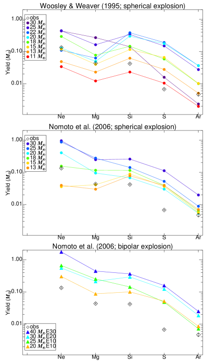
Figure 12.— Supernova yields and the masses of the X-ray-emitting elements (diamonds with error bars). The model yields of different progenitor masses (dots for spherical explosion and triangle for bipolar explosion) are taken from the core-collapse nucleosynthesis models of Woosley & Weaver (1995) and Nomoto et al. (2006). The bottom panel shows the yields from bipolar models with the kinetic energy enhanced by a factor of 10–30 (e.g., E20 stands for $E=20\times 10^{51}$ erg).

Kes 79 hosts a CCO, PSR J1852+0040, which is strong evidence of core-collapse explosion. Therefore, its progenitor is a massive ($\gtrsim 8~{}M_{\odot}$) star born in the MCs. During its short lifetime ($\sim 10^{6}$–$10^{7}$ years in the main-sequence stage; Schaller et al. 1992), the massive progenitor launches a strong stellar wind which blows a stellar wind bubble and sculpts the parent MCs. The SNR expanding inside the bubble may finally interact with the molecular cavity wall if the MC has not been dissipated, and actually several such SNRs have been revealed during the past several decades (see Chen et al. 2014; Zhang et al. 2015 and references therein). Chen et al. (2013) found a linear relationship between the size of the massive star’s molecular cavity and the star’s initial mass ($R_{\rm b}$–$M$ relation): $p_{5}^{1/3}R_{\rm b}\approx\alpha M-\beta$ pc, where $\alpha=1.22\pm 0.05$, $\beta=9.16\pm 1.77$, $p_{5}\equiv(p/k)/(10^{5}\,{\rm cm}^{-3}\,{\rm K})$, with the mean pressure $p/k$ in the MCs about $10^{5}\,{\rm cm}^{-3}\,{\rm K}$. This relation can be used to estimate the initial masses of the progenitors for SNRs interacting with molecular cavity walls or shells. Kes 79 is associated with the MCs in the velocity range of 95-115 $\,{\rm km}\,{\rm s}^{-1}$, and the molecular shell delineates the western radio outer shell and confines the middle shell. If the smaller hemisphere corresponding to the bright X-ray/IR filaments is in contact with the molecular cavity created by the progenitor’s stellar wind, we can adopt $R_{\rm b}\geq R_{1}\sim 4^{\prime}$ (8.3 pc; we use $\geq$ here since part of the wind energy may leak into the tenuous medium). The progenitor mass of Kes 79 is thus estimated to be $\geq 14\pm 2~{}M_{\odot}$.

Another method to estimate the progenitor mass is to compare the metal compositions inferred from the X-ray spectra with those predicted in the nucleosynthesis models. This method requires that different metal species are well mixed and observed, if the abundances from the global gas properties are used for comparison. According to the XMM-Newton spectral analysis of the global hot gas, Kes 79 has enriched Ne (1.8), Mg (1.6), Si (1.4) , S (1.7), and Ar ($\sim 1.8$). We first compare the best-fit abundances of Ne, Mg, S, and Ar relative to Si (e.g, [Ar/Si]/[Ar/Si]_⊙) in Kes 79 to those produced by the progenitors with different masses based on the spherical core-collapse nucleosynthesis models of Nomoto et al. (2006) and Woosley & Weaver (1995). Differences between the two models are discussed by Kumar et al. (2014; see also Kumar et al. 2012). However, we find that none of the available nucleosynthesis models can explain all of the observed metal abundance ratios for this SNR.

We subsequently compare the element masses in the X-ray-emitting gas with the predicted SN yields in the two nucleosynthesis models, which can provide at least a lower limit of the SNR’s progenitor mass. The element ($Z$) mass $M_{Z}$ is estimated from the abundance $A_{Z}$ and the mass of the hot component $M_{\rm h}$ ($=42\pm 1M_{\odot}$): $M_{Z}=A_{Z}M_{\rm h}(M_{Z\odot}/M_{\odot})$, where $(M_{Z\odot}/M_{\odot})$ is the solar mass fraction of the metal $Z$ adopted from Anders & Grevesse (1989). As shown in Figure 12, a progenitor mass less than $15~{}M_{\odot}$ can be excluded (spherical explosion models), since the mass of observed Ne exceeds that predicted in the $\leq 15~{}M_{\odot}$ yield models. It is consistent with the value $\geq 14\pm 2~{}M_{\odot}$ given by the $R_{\rm b}$–$M$ relation (discussed above). The observed metal masses are no larger than the 20 $M_{\odot}$ yield models for either the spherical or bipolar explosion (hypernova model with kinetic energy 10–30 times of the typical value of $10^{51}$ erg) scenarios. Under the assumption that most of the ejecta are observed in the X-ray band and that the Ne and Mg are well mixed in the SNR, the progenitor mass of Kes 79 is likely between 15 and 20 $M_{\odot}$.

However, the element masses are not consistent with any group of the modeled nucleosynthesis yields. The first explanation is that the ejecta are not well mixed or asymmetrically distributed in the SNR. Asymmetric distribution of ejecta is present in the SNR as discussed in Section 4.3. An alternative reason might be that Kes 79 is born from an asymmetric explosion with normal kinetic energy ($\sim 10^{51}$ erg) and the ejecta abundances cannot be explained with current spherical explosion or hypernova bipolar explosion model. Last but not least, the available nucleosynthesis models do not consistently provide similar yields, partly because of the assumptions made in the calculations. Future detailed models incorporating mildly asymmetric explosions and binary evolution are desirable to provide a more secure constraint on the progenitor of Kes 79 and other SNRs.

5. Summary

We have investigated the multi-wavelength emission from the thermal composite SNR Kes 79. Using the multi-transition CO data covering the whole SNR, we study the large-scale molecular environment as well as the small-scale structures which cause the asymmetries of the SNR. We also revisit the 380 ks XMM-Newton MOS data and carry out imaging and spectroscopic analysis of the X-ray-emitting plasma. The combined long-exposure X-ray data allow us to study the detailed distribution of different elements and the hot gas properties across the SNR. The main results are summarized as follows.

1. We provide kinematic and morphological evidence to support the interaction of SNR Kes 79 with the MCs in the velocity range 95-115 $\,{\rm km}\,{\rm s}^{-1}$: (1) broadened ¹²CO $J=3$–2 line ($\Delta v\approx 12~{}\,{\rm km}\,{\rm s}^{-1}$) is detected for the first time near the protrusion at the northeastern radio boundary; (2) the morphology agreement between the two ¹²CO $J=3$–2 filaments and the radio/IR/X-ray filaments in the east, and between the western molecular shell and the radio shells; and (3) the red-shifted ¹²CO lines relative to ¹³CO, suggesting an interaction with the MCs from the foreground SNR. The molecular gas region (mostly inside a $22^{\prime}$ region) near Kes 79 has a mass of $\sim 5.7d_{7.1}^{2}\times 10^{4}~{}M_{\odot}$, which is typical for a GMC.

2. The overall X-ray-emitting gas can be characterized by a cool ($kT_{\rm c}=0.195^{+0.003}_{-0.002}$ keV) under-ionized plasma with $\tau_{\rm h}=6.4\pm 0.4\times 10^{11}~{}\,{\rm cm}^{-3}\,{\rm s}$ and solar abundances, plus a hot ($kT_{\rm h}=0.80\pm 0.01$ keV) plasma with ionization timescale of $\tau_{\rm h}=8.1\pm 0.1\times 10^{10}\,{\rm cm}^{-3}\,{\rm s}$ and elevated Ne ($1.83^{+0.04}_{-0.05}$), Mg ($1.56\pm 0.03$ ), Si ($1.40\pm 0.02$), S ($1.72\pm 0.03$), and Ar ($1.8\pm 0.1$) abundances. The average densities of the two components are $\sim 2~{}\,{\rm cm}^{-3}$ and $\sim 0.5~{}\,{\rm cm}^{-3}$, respectively. The masses are $\sim 280~{}M_{\odot}$ and $\sim 40~{}M_{\odot}$, respectively. Hence, most of the X-ray emission is contributed by the shocked ISM. Kes 79 has a Sedov age of 4.4–6.7 kyr. The mean shock velocity is $7.3\times 10^{2}$ $\,{\rm km}\,{\rm s}^{-1}$.

3. The XMM-Newton image of Kes 79 reveals many bright X-ray filaments embedded in a faint halo. A two-temperature model (generally $kT_{\rm c}\sim 0.2$ keV and $kT_{\rm h}\sim 0.7$–1.0 keV) is required to describe the small-scale regions’ spectra all over the SNR. The filamentary gas has densities $\sim 4$–$13\,{\rm cm}^{-3}$ and $\sim 1$–$2~{}\,{\rm cm}^{-3}$ for the cool and hot components, respectively, which are much larger than those of the halo gas ($\sim 1.4$–$2.4~{}\,{\rm cm}^{-3}$ and $\sim 0.3$–$0.5~{}\,{\rm cm}^{-3}$ for the cool and hot components, respectively). The ionization ages of the hot component in the filaments (0.5–2.0 kyr) are smaller than in the halo ($\sim 4$–11 kyr). The X-ray-bright filaments are probably produced by the SNR interaction with the dense ambient gas, while the halo forms from SNR breaking out to a low-density medium.

4. The SNR shock propagating into the dense gas produces bright filamentary radiation in multiple wavelengths. The X-ray filaments show good spatial correlation with the 24 $\,\mu\rm m$ IR filaments and part of the radio shells. The filamentary mid-IR emission may come from the dust grains collisionally heated by the hot plasma.

5. Due to shaping by the inhomogeneous environment, Kes 79 is likely to have a double-hemisphere morphology. The smaller hemisphere containing bright filaments is at the back side and projected into the SNR interior. Projection effect can explain the multiple-shell structures and the thermal composite morphology of Kes 79.

6. We find a high-velocity ejecta fragment which shows distinctly high temperature ($kT_{\rm h}\sim 1.6^{+0.6}_{-0.3}$ keV) and abundances of Ne ($4.4^{+3.5}_{-2.2}$), Mg ($3.6^{+1.7}_{-1.0}$), Si ($5.2^{+2.2}_{-1.3}$), S ($5.2^{+1.8}_{-1.1}$), and Ar ($4.2^{+2.4}_{-1.8}$). Its velocity ($1.0^{+0.2}_{-0.1}~{}\,{\rm km}\,{\rm s}^{-1}$) is 32% larger than the average velocity of the blast wave. The high-velocity ejecta fragment, in addition to the asymmetric metal distribution across the remnant, supports the idea that the SN explosion is intrinsically asymmetric.

7. The progenitor mass of Kes 79 is estimated to be 15–$20~{}M_{\odot}$ by using two methods: (1) the linear relation between the progenitor mass and the wind blown bubble size ($R_{\rm b}$–$M$ relation), and (2) a comparison between the metal masses and the yields predicted by nucleosynthesis models.

References

- Anders & Grevesse (1989) Anders, E., & Grevesse, N. 1989, Geochim. Cosmochim. Acta, 53, 197
- Andersen et al. (2011) Andersen, M., Rho, J., Reach, W. T., Hewitt, J. W., & Bernard, J. P. 2011, ApJ, 742, 7
- Aschenbach et al. (1995) Aschenbach, B., Egger, R., & Trümper, J. 1995, Nature, 373, 587
- Auchettl et al. (2014) Auchettl, K., Slane, P., & Castro, D. 2014, ApJ, 783, 32
- Balucinska-Church & McCammon (1992) Balucinska-Church, M., & McCammon, D. 1992, ApJ, 400, 699
- Borkowski et al. (2001) Borkowski, K. J., Lyerly, W. J., & Reynolds, S. P. 2001, ApJ, 548, 820
- Blondin et al. (1996) Blondin, J. M., Lundqvist, P., & Chevalier, R. A. 1996, ApJ, 472, 257
- Cappellari & Copin (2003) Cappellari, M., & Copin, Y. 2003, MNRAS, 342, 345
- Case & Bhattacharya (1998) Case, G. L., & Bhattacharya, D. 1998, ApJ, 504, 761
- Cesarsky et al. (1999) Cesarsky, D., Cox, P., Pineau des Forêts, G., et al. 1999, A&A, 348, 945
- Chen et al. (2004) Chen, Y., Su, Y., Slane, P. O., & Wang, Q. D. 2004, ApJ, 616, 885
- Chen et al. (2013) Chen, Y., Zhou, P., & Chu, Y.-H. 2013, ApJ, 769, L16
- Chen et al. (2014) Chen, Y., Jiang, B., Zhou, P., et al. 2014, IAU Symposium, 296, 170
- Cho et al. (2015) Cho, W., Kim, J., & Koo, B.-C. 2015, Journal of Korean Astronomical Society, 48, 139
- Dame et al. (2001) Dame, T. M., Hartmann, D., & Thaddeus, P. 2001, ApJ, 547, 792
- Dempsey et al. (2013) Dempsey, J. T., Thomas, H. S., & Currie, M. J. 2013, ApJS, 209, 8
- Denoyer (1979) Denoyer, L. K. 1979, ApJ, 232, L165
- Dickman (1978) Dickman, R. L. 1978, ApJS, 37, 407
- Diehl & Statler (2006) Diehl, S., & Statler, T. S. 2006, MNRAS, 368, 497
- Draine & McKee (1993) Draine, B. T., & McKee, C. F. 1993, ARA&A, 31, 373
- Dubner et al. (2000) Dubner, G. M., Velázquez, P. F., Goss, W. M., & Holdaway, M. A. 2000, AJ, 120, 1933
- Dwek (1987) Dwek, E. 1987, ApJ, 322, 812
- Ferrand & Safi-Harb (2012) Ferrand, G., & Safi-Harb, S. 2012, Advances in Space Research, 49, 1313
- Fesen & Gunderson (1996) Fesen, R. A., & Gunderson, K. S. 1996, ApJ, 470, 967
- Frail & Clifton (1989) Frail, D. A., & Clifton, T. R. 1989, ApJ, 336, 854
- Gaensler (1998) Gaensler, B. M. 1998, ApJ, 493, 781
- Giacani et al. (2009) Giacani, E., Smith, M. J. S., Dubner, G., et al. 2009, A&A, 507, 841
- Gooch (1996) Gooch, R. 1996, Astronomical Data Analysis Software and Systems V, 101, 80
- Gotthelf et al. (2005) Gotthelf, E. V., Halpern, J. P., & Seward, F. D. 2005, ApJ, 627, 390
- Green et al. (1997) Green, A. J., Frail, D. A., Goss, W. M., & Otrupcek, R. 1997, AJ, 114, 2058
- Green (1989) Green, D. A. 1989, MNRAS, 238, 737
- Green & Dewdney (1992) Green, D. A., & Dewdney, P. E. 1992, MNRAS, 254, 686
- Grefenstette et al. (2014) Grefenstette, B. W., Harrison, F. A., Boggs, S. E., et al. 2014, Nature, 506, 339
- Halpern et al. (2007) Halpern, J. P., Gotthelf, E. V., Camilo, F., & Seward, F. D. 2007, ApJ, 665, 1304
- Halpern & Gotthelf (2010) Halpern, J. P., & Gotthelf, E. V. 2010, ApJ, 709, 436
- Hollenbach & McKee (1979) Hollenbach, D., & McKee, C. F. 1979, ApJS, 41, 555
- Hwang et al. (2000) Hwang, U., Holt, S. S., & Petre, R. 2000, ApJ, 537, L119
- Jiang et al. (2010) Jiang, B., Chen, Y., Wang, J., et al. 2010, ApJ, 712, 1147
- Kawamura et al. (1998) Kawamura, A., Onishi, T., Yonekura, Y., et al. 1998, ApJS, 117, 387
- Kumar et al. (2014) Kumar, H. S., Safi-Harb, S., Slane, P. O., & Gotthelf, E. V. 2014, ApJ, 781, 41
- Kumar et al. (2012) Kumar, H. S., Safi-Harb, S., & Gonzalez, M. E. 2012, ApJ, 754, 96
- Lazendic et al. (2005) Lazendic, J. S., Slane, P. O., Hughes, J. P., Chen, Y., & Dame, T. M. 2005, ApJ, 618, 733
- Lopez et al. (2011) Lopez, L. A., Ramirez-Ruiz, E., Huppenkothen, D., Badenes, C., & Pooley, D. A. 2011, ApJ, 732, 114
- Meyer et al. (2015) Meyer, D. M.-A., Langer, N., Mackey, J., Velázquez, P. F., & Gusdorf, A. 2015, MNRAS, 450, 3080
- Neufeld et al. (2007) Neufeld, D. A., Hollenbach, D. J., Kaufman, M. J., et al. 2007, ApJ, 664, 890
- Nomoto et al. (2006) Nomoto, K., Tominaga, N., Umeda, H., Kobayashi, C., & Maeda, K. 2006, Nuclear Physics A, 777, 424
- Pineault et al. (1987) Pineault, S., Landecker, T. L., & Routledge, D. 1987, ApJ, 315, 580
- Reynolds & Moffett (1993) Reynolds, S. P., & Moffett, D. A. 1993, AJ, 105, 2226
- Rea et al. (2014) Rea, N., Viganò, D., Israel, G. L., Pons, J. A., & Torres, D. F. 2014, ApJ, 781, L17
- Reach & Rho (2000) Reach, W. T., & Rho, J. 2000, ApJ, 544, 843
- Reach et al. (2002) Reach, W. T., Rho, J., Jarrett, T. H., & Lagage, P.-O. 2002, ApJ, 564, 302
- Rho & Petre (1998) Rho, J., & Petre, R. 1998, ApJ, 503, L167
- Sault et al. (1995) Sault, R. J., Teuben, P. J., & Wright, M. C. H. 1995, Astronomical Data Analysis Software and Systems IV, 77, 433
- Schöier et al. (2005) Schöier, F. L., van der Tak, F. F. S., van Dishoeck, E. F., & Black, J. H. 2005, A&A, 432, 369
- Schaller et al. (1992) Schaller, G., Schaerer, D., Meynet, G., & Maeder, A. 1992, A&AS, 96, 269
- Sedov (1959) Sedov, L. I. 1959, Similarity and Dimensional Methods in Mechanics, New York: Academic Press, 1959,
- Seok et al. (2013) Seok, J. Y., Koo, B.-C., & Onaka, T. 2013, ApJ, 779, 134
- Seward et al. (2003) Seward, F. D., Slane, P. O., Smith, R. K., & Sun, M. 2003, ApJ, 584, 414
- Seward & Velusamy (1995) Seward, F. D., & Velusamy, T. 1995, ApJ, 439, 715
- Shan et al. (2012) Shan, W. L., Yang, J., Shi, S. C., et al. 2012, IEEE Trans. Terahertz Sci. Technol., 2, 593
- Sun et al. (2004) Sun, M., Seward, F. D., Smith, R. K., & Slane, P. O. 2004, ApJ, 605, 742
- Tenorio-Tagle et al. (1985) Tenorio-Tagle, G., Bodenheimer, P., & Yorke, H. W. 1985, A&A, 145, 70
- Troja et al. (2006) Troja, E., Bocchino, F., & Reale, F. 2006, ApJ, 649, 258
- Velusamy et al. (1991) Velusamy, T., Becker, R. H., & Seward, F. D. 1991, AJ, 102, 676
- West et al. (2015) West, J. L., Safi-Harb, S., Jaffe, T., et al. 2015, arXiv:1510.08536
- Woosley & Weaver (1995) Woosley, S. E., & Weaver, T. A. 1995, ApJS, 101, 181
- Zhang et al. (2015) Zhang, G.-Y., Chen, Y., Su, Y., et al. 2015, ApJ, 799, 103
- Zhou et al. (2014) Zhou, P., Chen, Y., Li, X.-D., et al. 2014, ApJ, 781, L16