Low-complexity Pruned 8-point DCT Approximations for Image Encoding

Abstract

Two multiplierless pruned 8-point discrete cosine transform (DCT) approximation are presented. Both transforms present lower arithmetic complexity than state-of-the-art methods. The performance of such new methods was assessed in the image compression context. A JPEG-like simulation was performed, demonstrating the adequateness and competitiveness of the introduced methods. Digital VLSI implementation in CMOS technology was also considered. Both presented methods were realized in Berkeley Emulation Engine (BEE3).

Keywords
Approximate discrete cosine transform, pruning, pruned DCT, HEVC

1 Introduction

Orthogonal transforms are useful tools in many scientific applications [1]. In particular, the discrete cosine transform (DCT) [2] plays an important role in digital signal processing. Due to the energy compaction property, which are close related to the Karuhnen-Loève transform (KLT) [3], the DCT is often used in data compression [4]. In fact, the DCT is adopted in many image and video compression standards, such as JPEG [5], MPEG [6, 7, 8], H.261 [9, 10], H.263 [11, 7], H.264/AVC [12, 13], and the high efficiency video coding (HEVC) [14, 15]. Due to its range of applications, efforts have been made over decades to develop fast algorithms to compute the DCT efficiently [4].

The theoretical multiplicative complexity minimum for the $N$-point DCT was derived by Winograd in [16]. For the 8-point DCT, such minimum consists of 11 multiplications, which is achieved by Loeffler DCT algorithm [17]. Consequently, new algorithms that could further and significantly reduce the computational cost of the exact DCT computation are not trivially attainable. In this scenario, low-complexity DCT approximations have been proposed for image and video compression applications, such as the classical signed DCT (SDCT) [18], the Lengwehasatit-Ortega DCT approximation (LODCT) [19], the Bouguezel-Ahmad-Swamy (BAS) series [20, 21, 22], and algorithms based on integer functions [23, 24, 25]. Such methods are often multiplierless operations leading to hardware realizations that offer adequate trade-offs between accuracy and complexity [26].

In some applications, most of the useful signal information is concentrated in the lower DCT coefficients. Furthermore, in data compression applications, high frequency coefficients are often zeroed by the quantization process [27, p. 586]. Then, computational savings may be attained by not computing DCT higher coefficients. This approach is called pruning and was first applied for the discrete Fourier transform (DFT) by Markel [28]. In this case, pruning consists of discarding input vector coefficients—time-domain pruning—and operations involving them are not computed. Alternatively, one can discard output vector coefficients—frequency-domain pruning. The well-known Goertzel algorithm for single component DFT computation [29, 30, 31] can be understood in this latter sense. Frequency-domain pruning has been recently considered for mixed-radix FFT algorithms [32], cognitive radio design [33], and wireless communications [34].

The DCT pruning algorithm was proposed by Wang [35]. Due to the DCT energy compaction property, pruning has been applied in frequency-domain by discarding transform-domain coefficients with the least amounts of energy [35]. In the context of wireless image sensor networks, Lecuire et al. extended the method for the 2-D case [36]. A pruned DCT approximation was proposed in [37] based on the DCT approximation method presented in [22].

In [38], an alternative architecture for HEVC was proposed. Such method maintains the wordlength fixed by means of discarding least significant bits, minimizing the computation at the expense of wordlength truncation. Although conceptually different, the approach described in [38] was also referred to as ‘pruning’, in contrast with the classic and more common usage of this terminology. In the current work, we employ ‘pruning’ in the same sense as in [35].

The aim of this work is to present new pruned DCT approximations with lower arithmetic complexity adequate for image coding and compression. A comprehensive arithmetic complexity assessment among several methods is presented. A JPEG-like image compression simulation based on the proposed tools is applied to several images for a performance evaluation. VLSI architectures for the new presented methods are also introduced.

2 Mathematical Background

2.1 Discrete Cosine Transform

There are eight types of DCT [4]. The most popular one is the type II DCT or DCT-II, which is the best approximation for the KLT for highly correlated signals, being widely employed for data compression [39]. In this work we refer to the DCT-II simply as DCT.

Let $\mathbf{x}=\left[x_{0}~{}x_{1}~{}\ldots~{}x_{N-1}\right]^{\top}$ be an input $N$-point vector. The DCT of $\mathbf{x}$ is defined as the output vector $\mathbf{X}=\left[X_{0}~{}X_{1}~{}\ldots~{}X_{N-1}\right]^{\top}$, whose components are given by

$$X_{k}\!=\!\alpha_{k}\sqrt{\frac{2}{N}}\sum_{n=0}^{N-1}x_{n}\cos\left[\frac{\left(n+\frac{1}{2}\right)k\pi}{N}\right]\!,k=0,1,\ldots,N\!-\!1,$$

where

$$\alpha_{k}=\begin{cases}\frac{1}{\sqrt{2}},&\text{if}~{}k=0,\\ 1,&\text{otherwise.}\end{cases}$$

Alternatively, above expression can be expressed in matrix format according to:

$$\mathbf{X}=\mathbf{C}\cdot\mathbf{x},$$ (1)

where $\mathbf{C}$ is the $N\times N$ DCT matrix, whose entries are given by

$$c_{k,n}=\alpha_{k}\cdot\sqrt{2/N}\cdot\cos\left[(n+1/2)k\pi/N\right],$$

$$k,n=0,1,\ldots,N-1.$$

Matrix $\mathbf{C}$ is orthogonal, i.e., it satisfies $\mathbf{C}^{-1}=\mathbf{C}^{\top}$. Thus, the inverse transformation is $\mathbf{x}=\mathbf{C}^{\top}\cdot\mathbf{X}$. Given an $N\times N$ matrix $\mathbf{A}$, its forward 2-D DCT is defined as the transform-domain matrix $\mathbf{B}$ furnished by

$$\mathbf{B}=\mathbf{C}\cdot\mathbf{A}\cdot\mathbf{C}^{\top}.$$

By using orthogonality property, the reverse 2-D $N$-point DCT is given by

$$\mathbf{A}=\mathbf{C}^{\top}\cdot\mathbf{B}\cdot\mathbf{C}.$$

The forward 2-D DCT can be computed by eight column-wise calls of the 1-D DCT to $\mathbf{A}$; then the resulting intermediate matrix is submitted to eight row-wise calls of the 1-D DCT.

2.2 DCT Approximations

A DCT approximation $\hat{\mathbf{C}}$ is a matrix with similar properties to the DCT, generally requiring lower computational cost. In general, an approximation is constituted by the product $\hat{\mathbf{C}}=\mathbf{S}\cdot\mathbf{T}$, where $\mathbf{T}$ is a low-complexity matrix and $\mathbf{S}$ is a scaling diagonal matrix, which effects orthogonality or quasi-orthogonality [25]. In the image compression context, matrix $\mathbf{S}$ does not contribute with any extra computation, since it can be merged into the quantization step of usual compression algorithms [20, 21, 24, 26].

Current literature contains several good approximations. In this work, we separate the following approximations for analysis: (i) the SDCT [18], which is a classic DCT approximation; (ii) the LODCT [19], due to its comparatively high performance; (iii) the BAS series of approximations [20, 21, 22]; (iv) the rounded DCT (RDCT) [23]; (v) the modified RDCT (MRDCT) [24], which has the lowest arithmetic complexity in the literature; and (vi) transformation matrices $\mathbf{T}_{4}$, $\mathbf{T}_{5}$ and $\mathbf{T}_{6}$ introduced in [25], which are fairly recently proposed methods with good performance and low complexity.

2.3 Pruning Exact and Approximate DCT

DCT pruning consists in discarding selected input or output vector components in (1), thus avoiding computations that require them. Mathematically, it corresponds to the elimination of rows or columns of $\mathbf{C}$. Such operations results in a possibly rectangular submatrix of the original matrix $\mathbf{C}$. Pruning is often realized in frequency-domain by means of computing only the $K<N$ transform coefficients that retain more energy. For the DCT, this corresponds to the low index coefficients of the 1-D transform and the upper-left coefficients of 2-D. The new transformation matrix for this particular pruning method is the $K\times N$ matrix $\mathbf{C}_{\langle K\rangle}$ given by

$$\mathbf{C}_{\left<K\right>}=\begin{bmatrix}c_{0,0}&c_{0,1}&\cdots&c_{0,N-1}\\ c_{1,0}&c_{1,1}&\cdots&c_{1,N-1}\\ \vdots&\vdots&\ddots&\vdots\\ c_{K-1,0}&c_{K-1,1}&\cdots&c_{K-1,N-1}\\ \end{bmatrix}$$ (2)

Therefore, the 2-D pruned DCT is computed as follows:

$$\tilde{\mathbf{B}}=\mathbf{C}_{\langle K\rangle}\cdot\mathbf{A}\cdot\mathbf{C}_{\langle K\rangle}^{\top}.$$ (3)

The resulting matrix $\tilde{\mathbf{B}}$ is a square matrix of size $K\times K$. Lecuire et al. [36] showed that the $K\times K$ square pattern at the upper-right corner leads to a better energy-distortion trade-off when compared to the alternative triangle pattern [40].

Pruning can be applied to DCT approximations by means of discarding matrix rows of $\mathbf{T}$ that correspond to low-energy coefficients. Thus, the pruned transformation is expressed according to:

$$\mathbf{T}_{\langle K\rangle}=\begin{bmatrix}t_{0,0}&t_{0,1}&\cdots&t_{0,N-1}\\ t_{1,0}&t_{1,1}&\cdots&t_{1,N-1}\\ \vdots&\vdots&\ddots&\vdots\\ t_{K-1,0}&t_{K-1,1}&\cdots&t_{K-1,N-1}\\ \end{bmatrix}.$$ (4)

Above transformation furnishes the pruned approximation DCT: $\hat{\mathbf{C}}_{\langle K\rangle}=\mathbf{S}_{\langle K\rangle}\cdot\mathbf{T}_{\langle K\rangle}$, where $\mathbf{S}_{\langle K\rangle}=\sqrt{\operatorname{diag}\left[\mathbf{T}_{\langle K\rangle}\cdot\mathbf{T}_{\langle K\rangle}^{\top}\right]^{-1}}$ and $\operatorname{diag}(\cdot)$ returns a diagonal matrix with the diagonal elements of its argument.

3 Proposed Pruned DCT Approximations

3.1 Pruned LODCT

Presenting good performance at image compression and energy compaction, the LODCT [19] is associated to the following transformation matrix:

$$\mathbf{W}=\begin{bmatrix}1&1&1&1&1&1&1&1\\ 1&1&1&0&0&-1&-1&-1\\ 1&\frac{1}{2}&-\frac{1}{2}&-1&-1&-\frac{1}{2}&\frac{1}{2}&1\\ 1&0&-1&-1&1&1&0&-1\\ 1&-1&-1&1&1&-1&-1&1\\ 1&-1&0&1&-1&0&1&-1\\ \frac{1}{2}&-1&1&-\frac{1}{2}&-\frac{1}{2}&1&-1&\frac{1}{2}\\ 0&-1&1&-1&1&-1&1&0\end{bmatrix}.$$ (5)

The implied approximation matrix is furnished by $\hat{\mathbf{C}}=\mathbf{S}\cdot\mathbf{W}$, where $\mathbf{S}=\operatorname{diag}\left(\frac{1}{\sqrt{8}},\frac{1}{\sqrt{6}},\frac{1}{\sqrt{5}},\frac{1}{\sqrt{6}},\frac{1}{\sqrt{8}},\frac{1}{\sqrt{6}},\frac{1}{\sqrt{5}},\frac{1}{\sqrt{6}}\right)$. The fast algorithm for $\mathbf{W}$ requires 24 additions and 2 bit-shift operations [19].

By analyzing fifty $512\times 512$ standard images from a public bank [41], we noticed that the LODCT can concentrate $\approx\!98.98\%$ of the average total image energy in the transform-domain upper-left square of size $K=4$. Thus, computational savings can be achieved by computing only the 16 lower frequency coefficients. Above facts lead to the following pruned transformation based on the LODCT:

$$\mathbf{W}_{\langle 4\rangle}=\begin{bmatrix}1&1&1&1&1&1&1&1\\ 1&1&1&0&0&-1&-1&-1\\ 1&\frac{1}{2}&-\frac{1}{2}&-1&-1&-\frac{1}{2}&\frac{1}{2}&1\\ 1&0&-1&-1&1&1&0&-1\end{bmatrix}.$$ (6)

The corresponding pruned approximation is: $\hat{\mathbf{C}}_{\langle 4\rangle}=\mathbf{S}_{\langle 4\rangle}\cdot\mathbf{W}_{\langle 4\rangle}$, where $\mathbf{S}_{\langle 4\rangle}=\operatorname{diag}\left(\frac{1}{\sqrt{8}},\frac{1}{\sqrt{2}},\frac{1}{2},\frac{1}{\sqrt{2}}\right)$. A fast algorithm flow graph for the pruned 1-D LODCT is shown in Figure 1, requiring only 18 additions and 1 bit-shift operation.

Figure 1: Fast algorithm for $\mathbf{W}_{\langle 4\rangle}$.

3.2 Pruned MRDCT

The MRDCT presents the lowest arithmetic complexity among the meaningful DCT approximation in literature [24]. It is associated to the following low-complexity matrix:

$$\mathbf{M}=\begin{bmatrix}1&1&1&1&1&1&1&1\\ 1&0&0&0&0&0&0&-1\\ 1&0&0&-1&-1&0&0&1\\ 0&0&-1&0&0&1&0&0\\ 1&-1&-1&1&1&-1&-1&1\\ 0&-1&0&0&0&0&1&0\\ 0&-1&1&0&0&1&-1&0\\ 0&0&0&-1&1&0&0&0\end{bmatrix}.$$

This matrix furnishes the DCT approximation given by $\tilde{\mathbf{C}}=\mathbf{D}\cdot\mathbf{M}$, where $\mathbf{D}=\operatorname{diag}\left(\frac{1}{\sqrt{8}},\frac{1}{\sqrt{2}},\frac{1}{2},\frac{1}{\sqrt{2}},\frac{1}{\sqrt{8}},\frac{1}{\sqrt{2}},\frac{1}{2},\frac{1}{\sqrt{2}}\right)$. Its fast algorithm presents only 14 additions [24].

We submitted the same above-mentioned set of fifty images to the MRDCT and we noticed that it can concentrate $\approx\!99.34\%$ of the total average energy in the upper-left square of size $K=6$. Then, we propose the following pruned $6\times 8$ matrix:

$$\mathbf{M}_{\langle 6\rangle}=\begin{bmatrix}1&1&1&1&1&1&1&1\\ 1&0&0&0&0&0&0&-1\\ 1&0&0&-1&-1&0&0&1\\ 0&0&-1&0&0&1&0&0\\ 1&-1&-1&1&1&-1&-1&1\\ 0&-1&0&0&0&0&1&0\end{bmatrix}.$$

The DCT approximation is given by $\tilde{\mathbf{C}}_{\langle 6\rangle}=\mathbf{D}_{\langle 6\rangle}\cdot\mathbf{M}_{\langle 6\rangle}$, where $\mathbf{D}_{\langle 6\rangle}=\operatorname{diag}\left(\frac{1}{\sqrt{8}},\frac{1}{\sqrt{2}},\frac{1}{2},\frac{1}{\sqrt{2}},\frac{1}{\sqrt{8}},\frac{1}{\sqrt{2}}\right)$. A fast algorithm for the pruned 1-D MRDCT is shown in Figure 2, requiring only 12 additions.

Figure 2: Fast algorithm for $\mathbf{M}_{\langle 6\rangle}$.

3.3 Inverse Transformation

The direct 2-D transformation for the pruned LODCT furnishes a $4\times 4$ matrix $\mathbf{B}=\hat{\mathbf{C}}_{\langle 4\rangle}\cdot\mathbf{A}\cdot\hat{\mathbf{C}}_{\langle 4\rangle}^{\top}$. These 16 coefficients retain most of the signal energy as represented by the original LODCT. Then, the inverse 2-D LODCT can be invoked as shown below:

$$\hat{\mathbf{A}}=\hat{\mathbf{C}}^{\top}\cdot\begin{bmatrix}\mathbf{B}&\mathbf{0}\\ \mathbf{0}&\mathbf{0}\end{bmatrix}_{8\times 8}\cdot\hat{\mathbf{C}},$$

where $\hat{\mathbf{C}}$ is the non-pruned LODCT matrix. Therefore, matrix $\hat{\mathbf{A}}$ is an approximation of $\mathbf{A}$. However, taking into account the zero element locations and the fact the $\hat{\mathbf{C}}_{\langle 4\rangle}$ consists of the first four rows of $\hat{\mathbf{C}}$, we have the following alternative expression: $\hat{\mathbf{A}}=\hat{\mathbf{C}}_{\langle 4\rangle}^{\top}\cdot\mathbf{B}\cdot\hat{\mathbf{C}}_{\langle 4\rangle}$, where $\hat{\mathbf{C}}_{\langle 4\rangle}$ is the proposed $4\times 8$ pruned LODCT matrix. Furthermore, matrix $\hat{\mathbf{C}}_{\langle 4\rangle}^{\top}$ is the Moore-Penrose generalized inverse of $\hat{\mathbf{C}}_{\langle 4\rangle}$ [42, p. 363] . The computation of the inverse pruned MRDCT follows the same rationale as described above.

3.4 Complexity Assessment

On account of (3), we have that 2-D pruned approximate DCT is computed after eight column-wise calls of the 1-D pruned approximate DCT and $K$ row-wise calls of the same transformation. Let $\operatorname{A}_{\text{1-D}}\left(\mathbf{T}_{\langle K\rangle}\right)$ be the additive complexity of $\mathbf{T}_{\langle K\rangle}$. Thus, the additive complexity of the 2-D pruned approximate DCT is given by:

$$\begin{split}\operatorname{A}_{\text{2-D}}\left(\mathbf{T}_{\langle K\rangle}\right)&=8\cdot\operatorname{A}_{\text{1-D}}\left(\mathbf{T}_{\langle K\rangle}\right)+K\cdot\operatorname{A}_{\text{1-D}}\left(\mathbf{T}_{\langle K\rangle}\right)\\ &=(8+K)\cdot\operatorname{A}_{\text{1-D}}\left(\mathbf{T}_{\langle K\rangle}\right).\end{split}$$ (7)

Considering the arithmetic complexity of several DCT approximations and (7), we assessed the arithmetic complexity of the proposed pruned approximations. Results are shown in Table 1.

Table 1: Complexity Assessment

Method	1-D			2-D
	Mult.	Add.	Shift	Mult.	Add.	Shift
Chen DCT [43]	16	26	0	256	416	0
SDCT [18]	0	24	0	0	384	0
BAS 2008 [20]	0	18	2	0	288	32
BAS 2009 [21]	0	18	0	0	288	0
BAS 2013 [22]	0	24	0	0	284	0
RDCT [23]	0	22	0	0	352	0
MRDCT [24]	0	14	0	0	224	0
LODCT [19]	0	24	2	0	384	32
$\mathbf{T}_{4}$ [25]	0	24	0	0	384	0
$\mathbf{T}_{5}$ [25]	0	24	4	0	384	64
$\mathbf{T}_{6}$ [25]	0	24	6	0	384	96
Proposed $\mathbf{W}_{\langle 4\rangle}$	0	18	1	0	216	12
Proposed $\mathbf{M}_{\langle 6\rangle}$	0	12	0	0	168	0

The proposed $\mathbf{W}_{\langle 4\rangle}$ has $43.75~{}\%$ less operations than the original 2-D LODCT. The proposed $\mathbf{M}_{\langle 6\rangle}$ attained the lowest additive complexity among the considered methods: 12 and 168 additions for the 1-D and 2-D cases, respectively. Such method presents $25.0~{}\%$ less additions than the 2-D case of the original MRDCT. Both pruned methods present lower additive complexity than any of the considered 2-D methods.

4 Image Compression

Again considering the discussed set of images described in Section 3, we performed a JPEG-like image compression simulation based on each method listed in Table 1  [18, 20, 21]. Each input image is subdivided into 8$\times$8 blocks, and each block is submitted to a particular 2-D transformation according to (3). Then, the resulting coefficients are quantized according to the standard quantization operation for luminance [44, p. 155]. The inverse operation is performed to reconstruct the compressed images.

Original and reconstructed images are compared quantitatively using the peak signal-to-noise ratio (PSNR) [44, p. 9] and the structural similarity (SSIM) [45] as figures of merit. Average measurements were considered. Table 2 shows the results. Figure 3 shows a qualitative evaluation of the proposed methods. Original uncompressed and compressed Lena images obtained by means of the exact DCT and the proposed methods are depicted. PSNR and SSIM measurements are included for comparison. Notice that the such values relate to these particular images, whereas the measurements presented in Table II consists of the average values of the considered image set.

Table 2: Performance assessment

Method	PSNR	SSIM
Exact DCT [43]	33.1276	0.9030
SDCT [18]	29.8442	0.8356
BAS-2008 [20]	32.2017	0.8851
BAS-2009 [21]	31.7557	0.8763
BAS-2013 [22]	31.8416	0.8815
RDCT [23]	31.9553	0.8823
MRDCT [24]	30.9775	0.8552
LODCT. [19]	32.4364	0.8916
$\mathbf{T}_{4}$ [25]	31.9826	0.8823
$\mathbf{T}_{4}$ [25]	31.8422	0.8796
$\mathbf{T}_{5}$ [25]	32.2892	0.8892
Proposed $\mathbf{W}_{\langle 4\rangle}$	29.5282	0.8411
Proposed $\mathbf{M}_{\langle 6\rangle}$	29.5810	0.8349

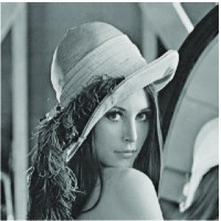
(a) Uncompressed

(b) Exact DCT (PSNR=35.8279, SSIM= 0.9192)

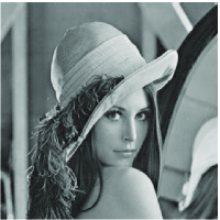
(c) Proposed $\mathbf{W}_{\langle 4\rangle}$ (PSNR=32.1736, SSIM= 0.8855)

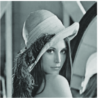
(d) Proposed $\mathbf{M}_{\langle 6\rangle}$ (PSNR=31.6174, SSIM= 0.8647)

(e) Uncompressed

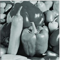
(f) Exact DCT (PSNR=34.7802, SSIM= 0.8814)

(g) Proposed $\mathbf{W}_{\langle 4\rangle}$ (PSNR=30.4485, SSIM= 0.8661)

(h) Proposed $\mathbf{M}_{\langle 6\rangle}$(PSNR=31.5742, SSIM= 0.8380)

Figure 3: Original and reconstructed Lena and peppers image according to exact DCT and the pruned proposed methods.

5 VLSI Architectures

In this section, hardware architectures for the proposed pruned LODCT and pruned MRDCT are detailed. The 1-D version of each transformation were initially modeled and tested in Matlab Simulink. Figure 4 and 5 depict the resulting architectures for the pruned LODCT and pruned MRDCT, respectively.

Figure 4: 1-D architecture of the proposed 8-point pruned LODCT.

Figure 5: 1-D architecture of the proposed 8-point pruned MRDCT.

5.1 FPGA Implementations

The above discussed architectures were physically realized on Berkeley Emulation Engine (BEE3) [46], a multi-FPGA based rapid prototyping system and was tested using on-chip hardware-in-the-loop co-simulation. The BEE3 system consists of a 2U chassis with a tightly-couple four FPGA system, widely employed in academia and industry. The main printed circuit Board (PCB) and a control & I/O PCB supports four Xilinx Virtex 5 FPGAs, up to 16 DDR2 DIMMs, eight 10GBase-CX4 Interfaces, four PCI-Express slots, four USB ports, four 1GbE RJ45 Ports, and one Xilinx USB-JTAG Interface, as illustrated in Figure 6. Such device was employed to physically realize the above architectures with fine-grain pipelining for increased throughput. FPGA realizations were tested with 10,000 random 8-point input test vectors. Test vectors were generated from within the MATLAB environment and routed to the BEE3 device through the USB ports and then measured data from the BEE3 device was routed back to MATLAB memory space.

\begin{picture}(7299.0,6000.0)(-23.0,-5161.0)\end{picture}

Figure 6: BEE3 device used to implement the architectures. Labels A, B, C, and D indicate the four Xilinx Virtex-5 XC5VSX95T-2FF1136 FPGA devices.

Evaluation of hardware complexity and real time performance considered the following metrics: the number of used configurable logic blocks (CLB), flip-flop (FF) count, critical path delay ($T_{\text{cpd}}$), and the maximum operating frequency ($F_{\text{max}}$) in MHz. The xflow.results report file was accessed to obtain the above results. Dynamic ($D_{p}$) and static power ($Q_{p}$) consumptions were estimated using the Xilinx XPower Analyzer for the Xilinx Virtex-5 XC5VSX95T-2FF1136 device. Results are shown in Table 3.

Table 3: Hardware resource consumption using Xilinx Virtex-5 XC5VSX95T-2FF1136 device

	Method
Hardware metric	Pruned LODCT	Pruned MRDCT
CLB	298	232
FF	1054	895
$T_{\text{cpd}}$ ($\mathrm{ns}$)	3.578	3.588
$F_{\text{max}}$ ($\mathrm{MHz}$)	279.48	278.70
$D_{p}$ ($\mathrm{mW/MHz}$)	3.141	3.620
$Q_{p}$ ($\mathrm{W}$)	1.50	1.50

6 Conclusion

In this paper, we introduced two pruning-based DCT approximations with very low arithmetic complexity. The resulting transformations require lower additive complexity than state-of-the-art methods. An image compression simulation were performed. Quantitative and qualitative assessments according to well-established figures of merits indicate the adequateness of the proposed methods. VLSI hardware realizations were proposed demonstrating the practicability of the proposed approximations.

References

- [1] N. Ahmed and K. R. Rao, Orthogonal Transforms for Digital Signal Processing. Springer, 1975.
- [2] K. R. Rao and P. Yip, Discrete Cosine Transform: Algorithms, Advantages, Applications. San Diego, CA: Academic Press, 1990.
- [3] N. Ahmed, T. Natarajan, and K. R. Rao, “Discrete cosine transform,” IEEE Transactions on Computers, vol. C-23, no. 1, pp. 90–93, Jan. 1974.
- [4] V. Britanak, P. Yip, and K. R. Rao, Discrete Cosine and Sine Transforms. Academic Press, 2007.
- [5] G. Wallace, “The JPEG still picture compression standard,” IEEE Transactions on Consumer Electronics, vol. 38, no. 1, pp. xviii–xxxiv, 1992.
- [6] D. J. L. Gall, “The MPEG video compression algorithm,” Signal Processing: Image Communication, vol. 4, pp. 129–140, 1992.
- [7] N. Roma and L. Sousa, “Efficient hybrid DCT-domain algorithm for video spatial downscaling,” EURASIP Journal on Advances in Signal Processing, vol. 2007, no. 2, pp. 30–30, 2007.
- [8] International Organisation for Standardisation, “Generic coding of moving pictures and associated audio information – Part 2: Video,” ISO, ISO/IEC JTC1/SC29/WG11 - Coding of Moving Pictures and Audio, 1994.
- [9] International Telecommunication Union, “ITU-T recommendation H.261 version 1: Video codec for audiovisual services at kbits,” ITU-T, Tech. Rep., 1990.
- [10] M. L. Liou, “Visual telephony as an ISDN application,” IEEE Communications Magazine, vol. 28, pp. 30–38, 1990.
- [11] International Telecommunication Union, “ITU-T recommendation H.263 version 1: Video coding for low bit rate communication,” ITU-T, Tech. Rep., 1995.
- [12] T. Wiegand, G. J. Sullivan, G. Bjontegaard, and A. Luthra, “Overview of the H.264/AVC video coding standard,” IEEE Transactions on Circuits and Systems for Video Technology, vol. 13, no. 7, pp. 560–576, Jul. 2003.
- [13] J. V. Team, “Recommendation H.264 and ISO/IEC 14 496–10 AVC: Draft ITU-T recommendation and final draft international standard of joint video specification,” ITU-T, Tech. Rep., 2003.
- [14] International Telecommunication Union, “High efficiency video coding: Recommendation ITU-T H.265,” ITU-T Series H: Audiovisual and Multimedia Systems, Tech. Rep., 2013.
- [15] M. T. Pourazad, C. Doutre, M. Azimi, and P. Nasiopoulos, “HEVC: The new gold standard for video compression: How does HEVC compare with H.264/AVC?” IEEE Consumer Electronics Magazine, vol. 1, no. 3, pp. 36–46, Jul. 2012.
- [16] S. Winograd, Arithmetic Complexity of Computations. CBMS-NSF Regional Conference Series in Applied Mathematics, 1980.
- [17] C. Loeffler, A. Ligtenberg, and G. S. Moschytz, “Practical fast 1-D DCT algorithms with 11 multiplications,” ICASSP International Conference on Acoustics, Speech, and Signal Processing, vol. 2, pp. 988–991, 1989.
- [18] T. I. Haweel, “A new square wave transform based on the DCT,” Signal Processing, vol. 82, pp. 2309–2319, 2001.
- [19] K. Lengwehasatit and A. Ortega, “Scalable variable complexity approximate forward DCT,” IEEE Transactions on Circuits and Systems for Video Technology, vol. 14, no. 11, pp. 1236–1248, Nov. 2004.
- [20] S. Bouguezel, M. O. Ahmad, and M. N. S. Swamy, “Low-complexity 88 transform for image compression,” Electronics Letters, vol. 44, no. 21, pp. 1249–1250, Sep. 2008.
- [21] ——, “A fast 88 transform for image compression,” in 2009 International Conference on Microelectronics (ICM), Dec. 2009, pp. 74–77.
- [22] ——, “Binary discrete cosine and Hartley transforms,” IEEE Transactions on Circuits and Systems I: Regular Papers, vol. 60, no. 4, pp. 989–1002, 2013.
- [23] R. J. Cintra and F. M. Bayer, “A DCT approximation for image compression,” IEEE Signal Processing Letters, vol. 18, no. 10, pp. 579–582, Oct. 2011.
- [24] F. M. Bayer and R. J. Cintra, “DCT-like transform for image compression requires 14 additions only,” Electronics Letters, vol. 48, no. 15, pp. 919–921, 2012.
- [25] R. J. Cintra, F. M. Bayer, and C. J. Tablada, “Low-complexity 8-point DCT approximations based on integer functions,” Signal Processing, vol. 99, pp. 201–214, 2014.
- [26] U. S. Potluri, A. Madanayake, R. J. Cintra, F. M. Bayer, S. Kulasekera, and A. Edirisuriya, “Improved 8-point approximate DCT for image and video compression requiring only 14 additions,” IEEE Transactions on Circuits and Systems I, vol. PP, pp. 1–14, Apr. 2014.
- [27] H. Malepati, Digital Media Processing: DSP Algorithms Using C. Newnes, 2010.
- [28] J. Markel, “FFT pruning,” IEEE Transactions on Audio and Electroacoustics, vol. 19, pp. 305–311, 1971.
- [29] A. Oppenheim and R. Schafer, Discrete-Time Signal Processing, 3rd ed. Pearson, 2010.
- [30] J.-H. Kim, J.-G. Kim, Y.-H. Ji, Y.-C. Jung, and C.-Y. Won, “An islanding detection method for a grid-connected system based on the Goertzel algorithm,” IEEE Transactions on Power Electronics, vol. 26, no. 4, pp. 1049–1055, Apr. 2011.
- [31] I. Carugati, S. Maestri, P. Donato, D. Carrica, and M. Benedetti, “Variable sampling period filter PLL for distorted three-phase systems,” IEEE Transactions on Power Electronics, vol. 27, no. 1, pp. 321–330, Jan. 2012.
- [32] L. Wang, X. Zhou, G. Sobelman, and R. Liu, “Generic mixed-radix FFT pruning,” IEEE Signal Processing Letters, vol. 19, no. 3, pp. 167–170, Mar. 2012.
- [33] R. Airoldi, O. Anjum, F. Garzia, A. M. Wyglinski, and J. Nurmi, “Energy-efficient fast Fourier transforms for cognitive radio systems,” IEEE Micro, vol. 30, no. 6, pp. 66–76, Nov. 2010.
- [34] P. Whatmough, M. Perrett, S. Isam, and I. Darwazeh, “VLSI architecture for a reconfigurable spectrally efficient FDM baseband transmitter,” IEEE Transactions on Circuits and Systems I: Regular Papers, vol. 59, no. 5, pp. 1107–1118, May 2012.
- [35] Z. Wang, “Pruning the fast discrete cosine transform,” IEEE Transactions on Communications, vol. 39, no. 5, pp. 640–643, May 1991.
- [36] V. Lecuire, L. Makkaoui, and J.-M. Moureaux, “Fast zonal DCT for energy conservation in wireless image sensor networks,” Electronics Letters, vol. 48, no. 2, pp. 125–127, 2012.
- [37] N. Kouadria, N. Doghmane, D. Messadeg, and S. Harize, “Low complexity DCT for image compression in wireless visual sensor networks,” Electronics Letters, vol. 49, no. 24, pp. 1531–1532, 2013.
- [38] P. Meher, S. Y. Park, B. Mohanty, K. S. Lim, and C. Yeo, “Efficient integer DCT architectures for HEVC,” Circuits and Systems for Video Technology, IEEE Transactions on, vol. 24, no. 1, pp. 168–178, Jan. 2014.
- [39] K. R. Rao and P. Yip, The Transform and Data Compression Handbook. CRC Press LLC, 2001.
- [40] L. Makkaoui, V. Lecuire, and J. Moureaux, “Fast zonal DCT-based image compression for wireless camera sensor networks,” 2nd International Conference on Image Processing Theory Tools and Applications (IPTA), pp. 126–129, 2010.
- [41] USC-SIPI Image Database. Signal and Image Processing Institute. University of Southern California. [Online]. Available: http://sipi.use.edu/database/
- [42] D. S. Bernstein, Matrix Mathematics: Theory, Facts, and Formulas. Princeton University Press, 2009.
- [43] W. H. Chen, C. Smith, and S. Fralick, “A fast computational algorithm for the discrete cosine transform,” IEEE Transactions on Communications, vol. 25, no. 9, pp. 1004–1009, Sep. 1977.
- [44] V. Bhaskaran and K. Konstantinides, Image and Video Compression Standards. Boston: Kluwer Academic Publishers, 1997.
- [45] Z. Wang, A. C. Bovik, H. R. Sheikh, and E. P. Simoncelli, “Image quality assessment: from error visibility to structural similarity,” IEEE Transactions on Image Processing, vol. 13, no. 4, pp. 600–612, Apr. 2004.
- [46] BEEcube Inc. Berkeley Emulation Engine. [Online]. Available: http://www.beecube.com/