Vector Gaussian Rate-Distortion
with Variable Side Information

Abstract

We consider rate-distortion with two decoders, each with distinct side information. This problem is well understood when the side information at the decoders satisfies a certain degradedness condition. We consider cases in which this degradedness condition is violated but the source and the side information consist of jointly Gaussian vectors. We provide a hierarchy of four lower bounds on the optimal rate. These bounds are then used to determine the optimal rate for several classes of instances.

I Introduction

We consider a rate-distortion problem with multiple decoders, each with potentially different side information, as shown in Fig. 1. This problem, which is sometimes called the Heegard-Berger problem, is one of the most basic network information theory problems that is not well understood, and it can arise in a couple of ways. First, the side information may represent reconstructions of the source due to prior transmissions. If the decoders have received different transmissions in the past, either due to channel loss or because they are not always listening to the transmitter, then their side information will be different. Second, it can be viewed as an instance of a ``compound Wyner-Ziv,'' problem, in which there is in reality only one decoder, but the encoder is uncertain about its side information. The side information associated with different decoders in the problem could then represent the transmitter's view of the set of possible side information configurations at the decoder. The transmitter then seeks to construct a message that would work reasonably well for any of these possible side information configurations.

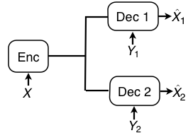
Figure 1: Problem Setup

The problem is well understood when the problem is degraded, i.e., the side information at one of the decoders is stochastically degraded with respect to the other's [1]. Recently, the following class of instances, schemes for which are called index coding, has received particular attention [2, 3]. The source at each time step is a vector of independent and identically distributed (i.i.d.) bits, each side information variable is a subset of these bits, and the goal of each decoder is to losslessly reproduce a subset of the bits that are not contained in its side information. Treating the source as an i.i.d. vector of uniform bits is appropriate if the source is first compressed by an optimal rate-distortion encoder. Thus index coding implicitly assumes a separation-based architecture in which lossy compression is performed first and then the broadcasting with side information is performed at the bit level. Ideally, one would consider both types of coding jointly. In previous work [4], we studied the index coding problem using tools from network information theory, in contrast to most past work on index coding which used techniques from network coding and graph theory. One of the advantages of using network information-theoretic tools, which was not pursued in the previous work, is that it allows one to consider the problems of lossy compression and coding for side information together, by allowing for a richer class of source models and distortion constraints. Our goal in this paper is to study systems that involve both lossy compression and coding for side information.

We shall focus on the case in which the source and the side information at the decoders are all jointly Gaussian vectors. This class of instances is important in applications, since vector Gaussian sources are natural stepping stones on the path from discrete memoryless sources to more sophisticated models of multimedia. The vector Gaussian setup can also be motivated theoretically since, like index coding, it is one of the simplest classes of instances that are not degraded in general. We shall focus on the case of two decoders; unlike index coding, for vector Gaussian problems even the two-decoder case is nontrivial.

We provide a hierarchy of four lower bounds on the optimal rate. For three separate special cases, we show that at least one of the lower bounds matches the best-known achievable rate [5, 1], thereby determining the optimal rate. The four lower bounds are all obtained using variations on the following argument. Since the rate-distortion function is known when the side information is degraded [1], a natural approach to proving lower bounds is to enhance the side information of one encoder or the other in order to make the problem degraded. The optimal rate for the newly-obtained instance is thus known and provides a lower bound on the optimal rate for the original instance. This idea can be applied several ways, leading to lower bounds of varying strength and usability. The weakest of these bounds is quite weak but also quite simple. The strongest, on the other hand, is quite strong but also difficult to apply. The intermediate bounds attempt to provide the best attributes of both.

We consider three different distortion constraints, all phrased as constraints on the error covariance matrices, averaged over the block, at the two decoders. The first stipulates an upper bound on the mean square error of the reproduction of each component of the source; this can be viewed as constraints on the diagonal elements of the time-average error covariance matrix. The second requires that the average error covariance matrix itself must be dominated, in a positive definite sense, by a given scaled identity matrix. In the final case, we require the trace of the average error covariance matrix to be upper bounded by a constant. For each of the three distortion measures, we solve a class of instances using the lower bounds developed in the paper. The necessary achievability arguments are standard, although our analysis does provide insight into how the auxiliary random variables therein should be chosen. Specifically, we show how to divide the signal space into ``regions,'' in which the side information at one decoder is ``stronger'' than that of the other. We then show that it is optimal for certain auxiliary random variables to live in certain of these regions.

The balance of the paper is organized as follows. The next two sections provide the problem formulation and the four lower bounds, respectively. Section IV contains the statements of our optimality results for all three cases described above. The achievability analysis for these problems is presented in Section V. Section VI shows how the lower bounds can be used to prove the converse half of the optimality results. Section VII contains a brief epilogue describing a conjectured difference among the lower bounds.

II Problem Definition

Let $\mathbf{X},\mathbf{Y_{1}},\mathbf{Y_{2}}$ be correlated vector Gaussian sources of size $k\times 1$, $k_{1}\times 1$ and $k_{2}\times 1$ respectively where $\mathbf{X}$ is the source to be compressed at the encoder and $\mathbf{Y_{1}}$ and $\mathbf{Y_{2}}$ comprise the side information at Decoder $1$ and Decoder $2$, respectively. We assume that the conditional covariance matrix of $\mathbf{X}$ given $\mathbf{Y_{i}}$, $K_{\mathbf{X}|\mathbf{Y_{i}}}$, $i\in\{1,2\}$ is invertible. Both Decoder $1$ and $2$ wish to reconstruct $\mathbf{X}$ subject to given distortion constraints. The objective is to characterize the rate distortion function for this setting. The following definitions are used to formulate the problem.

Definition 1.

$\Gamma_{i}$, $i\in\{1,2\}$ is defined as a mapping from the set of all $k\times k$ positive semi-definite (PSD) matrices to the set of $k_{0}\times k_{0}$ PSD matrices such that
1) $\Gamma_{i}(\cdot)$ is linear,
2) $A\preceq B$ implies that $\Gamma_{i}(A)\preceq\Gamma_{i}(B)$.

Definition 2.

An $(n,M,D_{1},D_{2})$ code where $D_{1}$ and $D_{2}$ are positive definite matrices, is composed of

• an encoding function

  $$f:\mathbb{R}^{kn}\rightarrow\{1,...,M\}$$

• and decoding functions

  $$g_{1} :\{1,...,M\}\times\mathbb{R}^{k_{1}n}\rightarrow\mathbb{R}^{kn}$$

  $$g_{2} :\{1,...,M\}\times\mathbb{R}^{k_{2}n}\rightarrow\mathbb{R}^{kn}$$

satisfying the distortion constraints

$$E\left[\frac{1}{n}\sum_{k=1}^{n}\Gamma_{i}\left((\mathbf{X}_{k}-\widehat{\mathbf{X}}_{\mathbf{i}k})(\mathbf{X}_{k}-\widehat{\mathbf{X}}_{\mathbf{i}k})^{T}\right)\right]\preceq D_{i},\ \ i\in\{1,2\}$$

where $\mathbf{\widehat{X}^{n}_{1}}=g_{1}(f(\mathbf{X^{n}}),\mathbf{Y_{1}^{n}})$, and $\mathbf{\widehat{X}^{n}_{2}}=g_{2}(f(\mathbf{X^{n}}),\mathbf{Y^{n}_{2}})$. We call $n$ the block length and $M$ the message size of the code.

Definition 3.

A rate $R$ is $(D_{1},D_{2})$-achievable if for every $\epsilon>0$, there exists an $(n,M,D_{1}+\epsilon I,D_{2}+\epsilon I)$ code such that $n^{-1}\log{M}\leq R+\epsilon$ .

Definition 4.

The rate-distortion function is defined as

$$R(\mathbf{D})=\inf\{R:R\textrm{ is }\mathbf{D}\textrm{-achievable}\},$$

where $\mathbf{D}=(D_{1},D_{2})$.

We shall prove our lower bounds for arbitrary distortion measures $\Gamma$ satisfying the requirements of Definition 1. We conclude this section by introducing the following notations used in rest of the paper.

Notation 1.

Let $\mathbf{X}$ be a $k\times 1$ vector where $k=l_{1}+l_{2}$. Then $(\mathbf{X})_{l_{1}}$ denotes the $l_{1}\times 1$ vector consisting of the first $l_{1}\times 1$ components of $\mathbf{X}$ and $[\mathbf{X}]_{l_{2}}$ denotes the remaining part of $\mathbf{X}$.

Notation 2.

Let $E$ be a $p\times p$ matrix. Then $(E)_{ij}$ denotes the element of $E$ which is in the $i^{th}$ row and $j^{th}$ column of $E$.

Notation 3.

Let $E$ and $F$ be $p\times p$ and $r\times r$ matrices where $p\geq l_{1}$ and $r\geq l_{2}$. Then $(E)_{l_{1}}$ denotes the upper-left $l_{1}\times l_{1}$ submatrix of $E$ and $[F]_{l_{2}}$ denotes the lower-right $l_{2}\times l_{2}$ submatrix of $F$.

Notation 4.

Let $E$ and $F$ be $p\times p$ and $r\times r$ matrices where $p\geq l_{1}$ and $r\geq l_{2}$. Then $(E)_{diag}$ denotes the $p\times p$ diagonal matrix whose diagonal elements are the same as that of $E$. Also, $(E)_{l_{1}diag}$ denotes the $l_{1}\times l_{1}$ diagonal matrix whose diagonal elements are the same as that of upper-left $l_{1}\times l_{1}$ submatrix of $E$ and $[F]_{l_{2}diag}$ denotes the $l_{2}\times l_{2}$ diagonal matrix whose diagonal elements are the same as that of lower-right $l_{2}\times l_{2}$ submatrix of $F$.

Notation 5.

Let $E$ and $F$ be $p\times p$ diagonal matrices. Then $\min\{E,F\}$ denotes the $p\times p$ diagonal matrix whose each diagonal entry is the minimum of corresponding diagonal entries of $E$ and $F$.

Notation 6.

Let $(\mathbf{X},\mathbf{\mathbf{Y}},\mathbf{Z})$ be a random vector. Then $\mathbf{X}\perp\mathbf{\mathbf{Y}}|\mathbf{Z}$ denotes that $\mathbf{X}$ and $\mathbf{\mathbf{Y}}$ are independent given $\mathbf{Z}$, $\mathbf{X}\leftrightarrow\mathbf{\mathbf{Y}}\leftrightarrow\mathbf{Z}$ denotes that $\mathbf{X}$, $\mathbf{\mathbf{Y}}$ and $\mathbf{Z}$ forms a Markov chain, and $K_{\mathbf{X}}$ denotes the covariance matrix of $\mathbf{X}$.

III Lower Bounds

We turn to lower bounds on the optimal rate. We shall provide four such bounds. In order of strongest (largest) to weakest (smallest), these are

1. The Minimax bound (mLB);

2. The Maximin bound (MLB);

3. The Enhanced-Enhancement bound (Enhanced-ELB or $\textsc{E}^{2}\textsc{LB}$);

4. The Enhancement bound (ELB).

Although the Maximin bound, the Enhanced-Enhancement bound, and the Enhancement bound are never larger than the Minimax bound, they are useful in that they are simpler to work with in some respects. We begin with the simplest, and weakest, of the bounds. This bound is folklore, and it turns out to be quite weak indeed.

III-A Enhancement Lower Bound

If the side information at the decoders is degraded, meaning that we can find a joint distribution of $(\mathbf{X},\mathbf{Y_{1}},\mathbf{Y_{2}})$ such that

$$\mathbf{X}\leftrightarrow\mathbf{Y_{\sigma(1)}}\leftrightarrow\mathbf{Y_{\sigma(2)}}$$ (1)

for some permutation $\sigma(.)$, then the rate distortion function is known [1, 5]. Hence a natural way to obtain a lower bound to $R(\mathbf{D})$ is to create degraded problems by providing extra side information to one decoder or the other. We call this lower bound enhancement lower bound, abbreviated as ELB, due to its similarity to the converse results for broadcast channels [6]. Proposition 1 states this lower bound.

Proposition 1.

The rate distortion function $R(\mathbf{D})$ is lower bounded by

$$R_{\textsc{ELB}}(\mathbf{D})=\max\{\sup_{S_{G}}\inf_{\widetilde{C}_{l1}(\mathbf{D})}R_{lo1},\sup_{S_{G}}\inf_{\widetilde{C}_{l2}(\mathbf{D})}R_{lo2}\},$$ (2)

where

$$R_{lo1} =I(\mathbf{X};\mathbf{W},\mathbf{U}|\mathbf{Y_{1}})+I(\mathbf{X};\mathbf{V}|\mathbf{W},\mathbf{U},\mathbf{Y}),$$ (3)

$$R_{lo2} =I(\mathbf{X};\mathbf{W},\mathbf{V}|\mathbf{Y_{2}})+I(\mathbf{X};\mathbf{U}|\mathbf{W},\mathbf{V},\mathbf{Y}),$$ (4)

$S_{G}=\{\mathbf{Y}\mbox{ jointly Gaussian with }(\mathbf{X},\mathbf{Y_{1}},\mathbf{Y_{2}})|\mathbf{X}\leftrightarrow\mathbf{Y}\leftrightarrow(\mathbf{Y_{1}},\mathbf{Y_{2}})\}$, and

$$\widetilde{C}_{l1}(\mathbf{D})\mbox{ is the set of }(\mathbf{W},\mathbf{U},\mathbf{V})\mbox{ such that } \widetilde{C}_{l2}(\mathbf{D})\mbox{ is the set of }(\mathbf{W},\mathbf{U},\mathbf{V})\mbox{ such that }$$

$$(\mathbf{W},\mathbf{U},\mathbf{V})\leftrightarrow\mathbf{X}\leftrightarrow(\mathbf{Y},\mathbf{Y_{1}},\mathbf{Y_{2}}) (\mathbf{W},\mathbf{U},\mathbf{V})\leftrightarrow\mathbf{X}\leftrightarrow(\mathbf{Y},\mathbf{Y_{1}},\mathbf{Y_{2}})$$

$$\Gamma_{1}\left(K_{\mathbf{X}|\mathbf{W},\mathbf{U},\mathbf{Y_{1}}}\right)\preceq D_{1},\mbox{ }\Gamma_{2}\left(K_{\mathbf{X}|\mathbf{W},\mathbf{U},\mathbf{V},\mathbf{Y}}\right)\preceq D_{2} \Gamma_{1}\left(K_{\mathbf{X}|\mathbf{W},\mathbf{U},\mathbf{V},\mathbf{Y}}\right)\preceq D_{1},\mbox{ }\Gamma_{2}\left(K_{\mathbf{X}|\mathbf{W},\mathbf{V},\mathbf{Y_{2}}}\right)\preceq D_{2}.$$

The ELB is quite weak. Consider, for example, what is arguably the simplest nontrivial instance of the problem: the source $\mathbf{X}$ is bivariate, $K_{\mathbf{X}}$, $K_{\mathbf{X}|\mathbf{Y_{1}}}$, and $K_{\mathbf{X}|\mathbf{Y}_{2}}$ are all diagonal, and the reconstructions at decoders are subject to component-wise MSE distortion constraints. This is essentially the parallel scalar Gaussian version of the problem. If the overall problem is degraded then the ELB is of course tight. But if one of the two components is degraded in one direction and the other component is degraded in the other, then Watanabe [7] has shown that the ELB is not tight, at least for the natural choice of $\mathbf{Y}$ that has

$$K_{\mathbf{X}|\mathbf{Y}}=\min\left(K_{\mathbf{X}|\mathbf{Y_{1}}},K_{\mathbf{X}|\mathbf{Y}_{2}}\right).$$

Comparing the ELB against the achievable bound in Theorem 5 to follow, one sees several potential sources of looseness. We shall see that the culprit is that the distortion constraints

$$\Gamma_{1}\left(K_{\mathbf{X}|\mathbf{W},\mathbf{U},\mathbf{Y_{1}}}\right) \preceq D_{1}$$

$$\Gamma_{2}\left(K_{\mathbf{X}|\mathbf{W},\mathbf{V},\mathbf{Y_{2}}}\right) \preceq D_{2}$$

in the achievable bound in Theorem 5 have been weakened to

$$\Gamma_{1}\left(K_{\mathbf{X}|\mathbf{W},\mathbf{U},\mathbf{V},\mathbf{Y}}\right) \preceq D_{1}$$

$$\Gamma_{2}\left(K_{\mathbf{X}|\mathbf{W},\mathbf{U},\mathbf{V},\mathbf{Y}}\right) \preceq D_{2}$$

here. Weakening the constraints in this way allows less informative $(\mathbf{W},\mathbf{U},\mathbf{V})$ to be feasible, because one can make use of the enhanced side information $\mathbf{Y}$ for estimation purposes. We shall make this intuition precise by showing that the Maximin and Enhanced-Enhancement lower bound, which differ from the ELB only in the distortion constraints, are tight for this problem. For reasons of expeditiousness, we shall state and prove the Minimax lower bound first, and then weaken it to obtain the Maximin and Enhanced-Enhancement lower bound.

III-B Minimax Lower Bound

Theorem 1 states the Minimax lower bound, abbreviated as mLB, to the rate distortion problem.

Theorem 1.

The rate distortion function, $R(\mathbf{D})$, is lower bounded by

$$R_{\textsc{mLB}}(\mathbf{D})=\sup_{S}\inf_{C_{l}(\mathbf{D})}\max\{R_{lo1},R_{lo2}\}$$ (5)

where $R_{lo1}$ and $R_{lo2}$ are as in (3) and (4), and

$$S=\{\mathbf{Y}|\mathbf{X}\leftrightarrow\mathbf{Y}\leftrightarrow(\mathbf{Y_{1}},\mathbf{Y_{2}})\}$$

$$C_{l}(\mathbf{D})\mbox{: the set of }(\mathbf{W},\mathbf{U},\mathbf{V})\mbox{ such that }$$

$$(\mathbf{W},\mathbf{U},\mathbf{V})\leftrightarrow\mathbf{X}\leftrightarrow(\mathbf{Y_{1}},\mathbf{Y_{2}},\mathbf{Y})$$

$$\Gamma_{1}\left(K_{\mathbf{X}|\mathbf{W},\mathbf{U},\mathbf{Y_{1}}}\right)\preceq D_{1},\Gamma_{2}\left(K_{\mathbf{X}|\mathbf{W},\mathbf{V},\mathbf{Y_{2}}}\right)\preceq D_{2}.$$

Proof of Theorem 1 .

By definition, for any $\mathbf{D}-$achievable rate, $R$, and for all $\epsilon>0$, we can find a $(n,2^{n(R+\epsilon)},\mathbf{D}+\epsilon(I,I))$ code. Let $\epsilon>0$ be given and $J$ denote the output of the encoder. Also let $\mathbf{Y}$ be an auxiliary source in $S$. Then, we can write

$$n(R+\epsilon) \geq H(J)$$

$$\geq I(\mathbf{X}^{n},\mathbf{Y}^{n}_{\mathbf{1}},\mathbf{Y}^{n};J)$$

$$\overset{a}{=}I(\mathbf{Y}^{n}_{\mathbf{1}};J)+I(\mathbf{Y}^{n};J|\mathbf{Y}^{n}_{\mathbf{1}})+I(\mathbf{X}^{n};J|\mathbf{Y}^{n}_{1},\mathbf{Y}^{n})$$

$$\geq I(\mathbf{Y}^{n};J|\mathbf{Y}^{n}_{\mathbf{1}})+I(\mathbf{X}^{n};J|\mathbf{Y}^{n}_{\mathbf{1}},\mathbf{Y}^{n})$$

$$\overset{b}{\geq}\sum^{n}_{i=1}\big{[}I(\mathbf{Y}_{i};J,\mathbf{Y}_{\mathbf{1}\leavevmode\hbox to2.34pt{\vbox to5.07pt{\text{[drawing]}}}}|\mathbf{Y}_{\mathbf{1}i})+I(\mathbf{X}_{i};J,\mathbf{Y}_{\mathbf{1}\leavevmode\hbox to2.34pt{\vbox to5.07pt{\text{[drawing]}}}},\mathbf{Y}_{\leavevmode\hbox to2.34pt{\vbox to5.07pt{\text{[drawing]}}}}|\mathbf{Y}_{\mathbf{1}i},\mathbf{Y}_{i})\big{]}$$ (6)

where $\mathbf{Y}_{\mathbf{1}\leavevmode\hbox to2.34pt{\vbox to5.07pt{\text{[drawing]}}}}$ denotes all $\mathbf{Y}^{n}_{\mathbf{1}}$ except $\mathbf{Y}_{1i}$ and $a$ is due to the chain rule, and $b$ is due to the chain rule and that conditioning reduces entropy. Then if we apply the chain rule to the last term above, the right hand side of (6) equals

$$\sum^{n}_{i=1}\big{[}I(\mathbf{Y}_{i};J,\mathbf{Y}_{\mathbf{1}\leavevmode\hbox to2.34pt{\vbox to5.07pt{\text{[drawing]}}}}|\mathbf{Y}_{\mathbf{1}i})+I(\mathbf{X}_{i};J,\mathbf{Y}_{\mathbf{1}\leavevmode\hbox to2.34pt{\vbox to5.07pt{\text{[drawing]}}}}|\mathbf{Y}_{\mathbf{1}i},\mathbf{Y}_{i})+I(\mathbf{X}_{i};\mathbf{Y}_{\leavevmode\hbox to2.34pt{\vbox to5.07pt{\text{[drawing]}}}}|J,\mathbf{Y}_{\mathbf{1}\leavevmode\hbox to2.34pt{\vbox to5.07pt{\text{[drawing]}}}},\mathbf{Y}_{\mathbf{1}i},\mathbf{Y}_{i})\big{]}$$ (7)

$$=\sum^{n}_{i=1}\big{[}I(\mathbf{X}_{i},\mathbf{Y}_{i};J,\mathbf{Y}_{\mathbf{1}\leavevmode\hbox to2.34pt{\vbox to5.07pt{\text{[drawing]}}}}|\mathbf{Y}_{\mathbf{1}i})+I(\mathbf{X}_{i};\mathbf{Y}_{\leavevmode\hbox to2.34pt{\vbox to5.07pt{\text{[drawing]}}}}|J,\mathbf{Y}_{\mathbf{1}\leavevmode\hbox to2.34pt{\vbox to5.07pt{\text{[drawing]}}}},\mathbf{Y}_{\mathbf{1}i},\mathbf{Y}_{i})\big{]}$$

$$\geq\sum^{n}_{i=1}\big{[}I(\mathbf{X}_{i};J,\mathbf{Y}_{\mathbf{1}\leavevmode\hbox to2.34pt{\vbox to5.07pt{\text{[drawing]}}}}|\mathbf{Y}_{1i})+I(\mathbf{X}_{i};\mathbf{Y}_{\leavevmode\hbox to2.34pt{\vbox to5.07pt{\text{[drawing]}}}}|J,\mathbf{Y}_{\mathbf{1}\leavevmode\hbox to2.34pt{\vbox to5.07pt{\text{[drawing]}}}},\mathbf{Y}_{\mathbf{1}i},\mathbf{Y}_{i})\big{]}.$$ (8)

Also, since $\mathbf{X}\leftrightarrow\mathbf{Y}\leftrightarrow(\mathbf{Y_{1}},\mathbf{Y_{2}})$ the right hand side of (8) is equal to

$$\sum^{n}_{i=1}\big{[}I(\mathbf{X}_{i};J,\mathbf{Y}_{\mathbf{1}\leavevmode\hbox to2.34pt{\vbox to5.07pt{\text{[drawing]}}}}|\mathbf{Y}_{\mathbf{1}i})+I(\mathbf{X}_{i};\mathbf{Y}_{\leavevmode\hbox to2.34pt{\vbox to5.07pt{\text{[drawing]}}}}|J,\mathbf{Y}_{\mathbf{1}\leavevmode\hbox to2.34pt{\vbox to5.07pt{\text{[drawing]}}}},\mathbf{Y}_{i})\big{]}$$

$${\geq}\sum^{n}_{i=1}\big{[}I(\mathbf{X}_{i};J,\mathbf{Y}_{\mathbf{1}\leavevmode\hbox to2.34pt{\vbox to5.07pt{\text{[drawing]}}}}|\mathbf{Y}_{\mathbf{1}i})+I(\mathbf{X}_{i};\mathbf{Y}_{\mathbf{2}{\leavevmode\hbox to2.34pt{\vbox to5.07pt{\text{[drawing]}}}}}|J,\mathbf{Y}_{\mathbf{1}\leavevmode\hbox to2.34pt{\vbox to5.07pt{\text{[drawing]}}}},\mathbf{Y}_{i})\big{]}$$

$${=}\sum^{n}_{i=1}\big{[}I(\mathbf{X}_{i};\mathbf{W^{\prime}}_{i},\mathbf{U^{\prime}}_{i}|\mathbf{Y}_{\mathbf{1}i})+I(\mathbf{X}_{i};\mathbf{V^{\prime}}_{i}|\mathbf{W^{\prime}}_{i},\mathbf{U^{\prime}}_{i},\mathbf{Y}_{i})\big{]}$$ (9)

where $\mathbf{W^{\prime}}_{i}=J$, $\mathbf{U^{\prime}}_{i}=\mathbf{Y}_{\mathbf{1}\leavevmode\hbox to2.34pt{\vbox to5.07pt{\text{[drawing]}}}}$ and $\mathbf{V^{\prime}}_{i}=\mathbf{Y}_{\mathbf{2}\leavevmode\hbox to2.34pt{\vbox to5.07pt{\text{[drawing]}}}}$. Note that $(\mathbf{W^{\prime}}_{i},\mathbf{U^{\prime}}_{i},\mathbf{V^{\prime}}_{i})\leftrightarrow\mathbf{X}_{i}\leftrightarrow(\mathbf{Y}_{\mathbf{1}i},\mathbf{Y}_{\mathbf{2}i},\mathbf{Y}_{i})$ for all $i\in[n]$. Let $T$ be a random variable uniformly distributed on $[n]$ and independent of the source, side information and all $(\mathbf{W}^{\prime}_{i},\mathbf{U}^{\prime}_{i},\mathbf{V}^{\prime}_{i})$, $i\in[n]$. Then we can write the right hand side of (9) as

$$\sum^{n}_{i=1}\big{[}I(\mathbf{X}_{i};\mathbf{W^{\prime}}_{i},\mathbf{U^{\prime}}_{i}|\mathbf{Y}_{\mathbf{1}i},T=i)+I(\mathbf{X}_{i};\mathbf{V^{\prime}}_{i}|\mathbf{W^{\prime}}_{i},\mathbf{U^{\prime}}_{i},\mathbf{Y}_{i},T=i)\big{]}$$

$$=n\big{[}I(\mathbf{X};\mathbf{W^{\prime}},\mathbf{U^{\prime}},T|\mathbf{Y}_{\mathbf{1}})+I(\mathbf{X};\mathbf{V^{\prime}},T|\mathbf{W^{\prime}},\mathbf{U^{\prime}},T,\mathbf{Y})\big{]}$$

$$=nR_{lo1},\mbox{ by denoting $(\mathbf{W^{\prime}},T)$, $(\mathbf{U^{\prime}},T)$, $(\mathbf{V^{\prime}},T)$ as $\mathbf{W}$, $\mathbf{U}$, $\mathbf{V}$ respectively.}$$ (10)

If we swap the role of $\mathbf{Y_{1}}$ and $\mathbf{Y_{2}}$ and apply the same procedure above, we can get

$$R+\epsilon \geq I(\mathbf{X};\mathbf{W},\mathbf{V}|\mathbf{Y}_{2})+I(\mathbf{X};\mathbf{U}|\mathbf{W},\mathbf{V},\mathbf{Y})$$

$$=R_{lo2}.$$ (11)

Note that since $(\mathbf{W^{\prime}}_{i},\mathbf{U^{\prime}}_{i},\mathbf{V^{\prime}}_{i})\leftrightarrow\mathbf{X}_{i}\leftrightarrow(\mathbf{Y}_{\mathbf{1}i},\mathbf{Y}_{\mathbf{2}i},\mathbf{Y}_{i})$ for all $i\in[n]$, we have $(\mathbf{W},\mathbf{U},\mathbf{V})\leftrightarrow\mathbf{X}\leftrightarrow(\mathbf{Y_{1}},\mathbf{Y_{2}},\mathbf{Y})$. Moreover since $(\mathbf{W^{\prime}}_{i},\mathbf{U^{\prime}}_{i},\mathbf{Y}_{\mathbf{1}i})=(J,\mathbf{Y}^{n}_{\mathbf{1}})$ and $(\mathbf{W^{\prime}}_{i},\mathbf{V^{\prime}}_{i},\mathbf{Y}_{\mathbf{2}i})=(J,\mathbf{Y}^{n}_{\mathbf{2}})$, given $(\mathbf{W^{\prime}}_{i},\mathbf{U^{\prime}}_{i},\mathbf{Y}_{\mathbf{1}i})$ Decoder $1$ can reconstruct the source, $\mathbf{X}_{i}$, subject to its distortion constraint. Similarly, Decoder $2$ can reconstruct the source, $\mathbf{X}_{i}$ given $(\mathbf{W^{\prime}}_{i},\mathbf{V^{\prime}}_{i},\mathbf{Y}_{\mathbf{2}i})$. Hence, $(\mathbf{W},\mathbf{U},\mathbf{V})\in C_{l}(\mathbf{D}+\epsilon(I,I))$ and we have

$$R(\mathbf{D})\geq\inf_{C_{l}(\mathbf{D}+\epsilon(I,I))}\max\{R_{lo1},R_{lo2}\}-\epsilon.$$ (12)

Let $R^{\prime}_{lo}(\mathbf{D}+\epsilon(I,I),\mathbf{Y})$ denote the right hand side of (12). Note that (12) holds for any $\mathbf{Y}\in S$, where $S$ as in Theorem 1. Hence we can write

$$R(\mathbf{D})\geq\sup_{S}R^{\prime}_{lo}(\mathbf{D}+\epsilon(I,I),\mathbf{Y})-\epsilon.$$ (13)

Note that from Lemma 9 in Appendix C, $R^{\prime}_{lo}(\mathbf{D},\mathbf{Y})$ is convex in $\mathbf{D}$. Since $0\prec D_{i}$, $i\in\{1,2\}$ we can find $\delta(D_{1},D_{2})>0$ such that $0\prec D_{i}-\delta(D_{1},D_{2})I$ for $i\in\{1,2\}$. Hence $R^{\prime}_{lo}(\mathbf{D}+\gamma(I,I),\mathbf{Y})$ is also convex in $\gamma$, where $\gamma\geq-\delta(D_{1},D_{2})$. Note that $\sup_{S}R^{\prime}_{lo}(\mathbf{D}+\epsilon(I,I),\mathbf{Y})$ is also convex since supremum of convex functions is convex. Then, we can conclude that $\sup_{S}R^{\prime}_{lo}(\mathbf{D}+\epsilon(I,I),\mathbf{Y})$ is continuous at $\epsilon=0$ since a convex function on an open set is continuous. Lastly, since $\epsilon$ was arbitrary, letting $\epsilon\rightarrow 0$ gives the result. ∎

It is worth noting that one can prove a bound similar to mLB for non-Gaussian sources and general additive distortion constraints. Although the mLB is quite powerful, it can be difficult to apply. In particular, it is not clear that it is sufficient to consider $(\mathbf{W},\mathbf{U},\mathbf{V})$ that are jointly Gaussian with $(\mathbf{X},\mathbf{Y}_{1},\mathbf{Y}_{2})$. Similarly, when considering the analogous form of this bound for discrete memoryless sources, it it not clear how to obtain cardinality bounds on the auxiliary random variables $(\mathbf{W},\mathbf{U},\mathbf{V})$. As such, it is not clear how to compute this bound in general. We shall therefore consider a slightly weakened form of the bound that is easier to apply. It turns out that simply swapping the $\min$ and the $\max$ in the objective and adding that $\mathbf{Y}$ is jointly Gaussian with $(\mathbf{X},\mathbf{Y_{1}},\mathbf{Y_{2}})$ to $S$ yields a bound that is significantly more tractable.

III-C Maximin Lower Bound

The next proposition gives the Maximin lower bound, abbreviated as MLB.

Proposition 2.

The rate distortion function, $R(\mathbf{D})$, is lower bounded by

$$R_{MLB}(\mathbf{D})=\max\{\sup_{S_{G}}\inf_{C_{l1}(\mathbf{D})}R_{lo1},\sup_{S_{G}}\inf_{C_{l2}(\mathbf{D})}R_{lo2}\},$$ (14)

where $R_{lo1}$ and $R_{lo2}$ are as in (3) and (4) respectively, $S_{G}$ as in Proposition 1, and

$$C_{l1}(\mathbf{D}):\mbox{ the set of }(\mathbf{W},\mathbf{U},\mathbf{V})\mbox{ such that } C_{l2}(\mathbf{D}):\mbox{ the set of }(\mathbf{W},\mathbf{U},\mathbf{V})\mbox{ such that }$$

$$(\mathbf{W},\mathbf{U},\mathbf{V})\leftrightarrow\mathbf{X}\leftrightarrow(\mathbf{Y_{1}},\mathbf{Y_{2}},\mathbf{Y}) (\mathbf{W},\mathbf{U},\mathbf{V})\leftrightarrow\mathbf{X}\leftrightarrow(\mathbf{Y_{1}},\mathbf{Y_{2}},\mathbf{Y})$$

$$\Gamma_{1}\left(K_{\mathbf{X}|\mathbf{W},\mathbf{U},\mathbf{Y_{1}}}\right)\preceq D_{1},\mbox{ }\Gamma_{2}\left(K_{\mathbf{X}|\mathbf{W},\mathbf{V},\mathbf{Y_{2}}}\right)\preceq D_{2} \Gamma_{1}\left(K_{\mathbf{X}|\mathbf{W},\mathbf{U},\mathbf{Y_{1}}}\right)\preceq D_{1},\mbox{ }\Gamma_{2}\left(K_{\mathbf{X}|\mathbf{W},\mathbf{V},\mathbf{Y_{2}}}\right)\preceq D_{2}.$$

Proof.

This follows directly from the mLB, Theorem 1, by moving the $\inf$ in the objective inside the maximization over the bounds in (3) and (4) and replacing the set $S$ with $S_{G}$. ∎

Although numerical evidence suggests that the MLB can be strictly weaker than the mLB (see the discussion in Section VII to follow), the MLB does have certain advantages. For the analogous bound for discrete memoryless sources with additive distortion measures, one can obtain cardinality bounds on the alphabets of $\mathbf{W}$, $\mathbf{U}$, and $\mathbf{V}$ using straightforward techniques [8]. And we shall show that, for the Gaussian form examined here, one may restrict attention to $\mathbf{W}$, $\mathbf{U}$, and $\mathbf{V}$ that are jointly Gaussian with $(\mathbf{X},\mathbf{Y}_{1},\mathbf{Y}_{2},\mathbf{Y})$.

Evidently the MLB differs from the ELB in Proposition 1 only in that the distortion constraints are replaced with those that appear in the achievable upper bound presented in Theorem 5 in Section V. In Section VI, we shall see that this improvement suffices to make the bound tight for the rate distortion problem with MSE distortion constraints stated in Section IV. We turn to the fourth and final lower bound.

III-D Enhanced-Enhancement Lower Bound

Proposition 3.

The rate distortion function, $R(\mathbf{D})$, is lower bounded by

$$R_{\textsc{E}^{2}\textsc{LB}}(\mathbf{D})=\max\{\sup_{S_{G}}\inf_{\bar{C}_{l1}(\mathbf{D})}R_{lo1},\sup_{S_{G}}\inf_{\bar{C}_{l2}(\mathbf{D})}R_{lo2}\},$$ (15)

where $R_{lo1}$ and $R_{lo2}$ are as in (3) and (4) respectively, $S_{G}$ as in Proposition 1, and

$$\bar{C}_{l1}(\mathbf{D}):\mbox{ the set of }(\mathbf{W},\mathbf{U},\mathbf{V})\mbox{ such that } \bar{C}_{l2}(\mathbf{D}):\mbox{the set of }(\mathbf{W},\mathbf{U},\mathbf{V})\mbox{ such that }$$

$$(\mathbf{W},\mathbf{U},\mathbf{V})\leftrightarrow\mathbf{X}\leftrightarrow(\mathbf{Y_{1}},\mathbf{Y_{2}},\mathbf{Y}) (\mathbf{W},\mathbf{U},\mathbf{V})\leftrightarrow\mathbf{X}\leftrightarrow(\mathbf{Y_{1}},\mathbf{Y_{2}},\mathbf{Y})$$

$$\Gamma_{1}\left(K_{\mathbf{X}|\mathbf{W},\mathbf{U},\mathbf{Y_{1}}}\right)\preceq D_{1}, \Gamma_{1}\left((K^{-1}_{\mathbf{X}|\mathbf{W},\mathbf{U},\mathbf{V},\mathbf{Y}}-\widehat{K})^{-1}\right)\preceq D_{1},$$

$$\Gamma_{2}\left((K^{-1}_{\mathbf{X}|\mathbf{W},\mathbf{U},\mathbf{V},\mathbf{Y}}-\widetilde{K})^{-1}\right)\preceq D_{2} \Gamma_{2}\left(K_{\mathbf{X}|\mathbf{W},\mathbf{V},\mathbf{Y_{2}}}\right)\preceq D_{2}$$

and $\widetilde{K}=K^{-1}_{\mathbf{X}|\mathbf{Y}}-K^{-1}_{\mathbf{X}|\mathbf{Y_{2}}}$, $\widehat{K}=K^{-1}_{\mathbf{X}|\mathbf{Y}}-K^{-1}_{\mathbf{X}|\mathbf{Y_{1}}}$.

Proof.

Note that only difference between MLB and Enhanced-ELB is the optimization sets over which the infima are taken. Hence it is enough to show that $C_{li}(\mathbf{D})\subseteq\bar{C}_{li}(\mathbf{D})$ for $i\in\{1,2\}$. Let $(\mathbf{W},\mathbf{U},\mathbf{V})\in C_{l1}(\mathbf{D})$. Then $(\mathbf{W},\mathbf{U},\mathbf{V})$ satisfy the Markov chain condition $(\mathbf{W},\mathbf{U},\mathbf{V})\leftrightarrow\mathbf{X}\leftrightarrow(\mathbf{Y_{1}},\mathbf{Y_{2}},\mathbf{Y})$ and we have $\Gamma_{1}\left(K_{\mathbf{X}|\mathbf{W},\mathbf{U},\mathbf{Y_{1}}}\right)\preceq D_{1}$. Also, the inequalities $K_{\mathbf{X}|\mathbf{W},\mathbf{U},\mathbf{V},\mathbf{Y_{2}}}\preceq K_{\mathbf{X}|\mathbf{W},\mathbf{V},\mathbf{Y_{2}}}$ and $K^{-1}_{\mathbf{X}|\mathbf{W},\mathbf{U},\mathbf{V},\mathbf{Y_{2}}}\preceq K^{-1}_{\mathbf{X}|\mathbf{W},\mathbf{U},\mathbf{V},\mathbf{Y}}-\widetilde{K}$ imply, by the Gaussian ``variance-drop'' lemma (Lemma 7 in Appendix A), that $\Gamma_{2}\left((K^{-1}_{\mathbf{X}|\mathbf{W},\mathbf{U},\mathbf{V},\mathbf{Y}}-\widetilde{K})^{-1}\right)\preceq D_{2}$. Hence $(\mathbf{W},\mathbf{U},\mathbf{V})$ is also in $\bar{C}_{l1}(\mathbf{D})$, giving $C_{l1}(\mathbf{D})\subseteq\bar{C}_{l1}(\mathbf{D})$. We can apply similar procedure to get $C_{l2}(\mathbf{D})\subseteq\bar{C}_{l2}(\mathbf{D})$, which concludes the proof. ∎

Comparing the Enhanced-ELB against the ELB in (2) shows that the differences lie entirely in the distortion constraints. The ELB effectively allows the decoders to use their ``enhanced'' side information for the purposes of estimating the source. The achievable bound, by contrast, does not. The Enhanced-ELB allows the decoders to use their enhanced side information, but it also tightens the constraint to account for this extra information, as justified by the Gaussian variance-drop lemma. We shall see in the next subsection that the Enhanced-ELB actually coincides with the MLB for all of the problems considered in this paper. We mention the Enhanced-ELB only because the idea of using the Gaussian variance-drop lemma to tighten the distortion constraints at decoders that are provided with improved side information may prove useful in other contexts.

III-E Properties of the Lower Bounds

It is evident from the proofs in this section that the four lower bounds can be ordered as follows

$$R_{\textsc{ELB}}(\mathbf{D})\leq R_{\textsc{E}^{2}\textsc{LB}}(\mathbf{D})\leq R_{\textsc{MLB}}(\mathbf{D})\leq R_{\textsc{mLB}}(\mathbf{D}).$$

We shall show that Gaussian auxiliary random variables are optimal for MLB, Enhanced-ELB, and ELB, and that the MLB and Enhanced-ELB are in fact equal. We begin by showing that Gaussian auxiliary random variables are optimal for the ELB and Enhanced-ELB.

Lemma 1.

One may add the constraint that $(\mathbf{W},\mathbf{U},\mathbf{V})$ is jointly Gaussian with $(\mathbf{X},\mathbf{Y}_{1},\mathbf{Y}_{2},\mathbf{Y})$ to the optimization problem in the ELB in (2) and the Enhanced-ELB in (15) without affecting the optimal value.

Proof.

See Appendix B. ∎

Proposition 4.

The Maximin bound and Enhanced-Enhancement bound in Proposition 2 and 3, respectively, coincide:

$$R_{\textsc{MLB}}(\mathbf{D})=R_{\textsc{E}^{2}\textsc{LB}}(\mathbf{D}).$$ (16)

Proof.

It suffices to show that

$$R_{\textsc{MLB}}(\mathbf{D})\leq R_{\textsc{E}^{2}\textsc{LB}}(\mathbf{D})$$

By Lemma 1, $(\mathbf{W},\mathbf{U},\mathbf{V})$ in $\bar{C}_{l1}(\mathbf{D})$ or $\bar{C}_{l2}(\mathbf{D})$ can be restricted to vector Gaussian random variables without loss of optimality. Furthermore, any $\mathbf{U}\in\bar{C}_{l1}$ can be lumped into $\mathbf{W}\in\bar{C}_{l1}(\mathbf{D})$, i.e. $\mathbf{U}$ is deterministic, without loss of optimality since $\mathbf{W}$ and $\mathbf{U}$ always appear together both in the objective and the conditions. The same argument holds when we swap the roles of $\mathbf{U}$ and $\mathbf{V}$ in $\bar{C}_{l2}(\mathbf{D})$. Hence, with those additional conditions we can write the optimizing sets, $\bar{C}_{l1}(\mathbf{D})$ and $\bar{C}_{l2}(\mathbf{D})$, as

$$\bar{C}_{l1}(\mathbf{D}): \bar{C}_{l1}(\mathbf{D}):$$

$$(\mathbf{W},\mathbf{U},\mathbf{V})\leftrightarrow\mathbf{X}\leftrightarrow(\mathbf{Y_{1}},\mathbf{Y_{2}},\mathbf{Y}) (\mathbf{W},\mathbf{U},\mathbf{V})\leftrightarrow\mathbf{X}\leftrightarrow(\mathbf{Y_{1}},\mathbf{Y_{2}},\mathbf{Y})$$

$$(\mathbf{W},\mathbf{U},\mathbf{V},\mathbf{X},\mathbf{Y_{1}},\mathbf{Y_{2}},\mathbf{Y})\mbox{ jointly Gaussian },\mathbf{U}=\emptyset (\mathbf{W},\mathbf{U},\mathbf{V},\mathbf{X},\mathbf{Y_{1}},\mathbf{Y_{2}},\mathbf{Y})\mbox{ jointly Gaussian },\mathbf{V}=\emptyset$$

$$K_{\mathbf{X}|\mathbf{W},\mathbf{Y_{1}}}\preceq D_{1},\mbox{ }K_{\mathbf{X}|\mathbf{W},\mathbf{V},\mathbf{Y_{2}}}\preceq D_{2} K_{\mathbf{X}|\mathbf{W},\mathbf{U},\mathbf{Y_{1}}}\preceq D_{1},\mbox{ }K_{\mathbf{X}|\mathbf{W},\mathbf{Y_{2}}}\preceq D_{2}$$

Then any such $(\mathbf{W},\mathbf{U},\mathbf{V})\in\bar{C}_{l1}(\mathbf{D})$ (or $(\mathbf{W},\mathbf{U},\mathbf{V})\in\bar{C}_{l2}(\mathbf{D})$) is also in ${C}_{l1}(\mathbf{D})$ (or ${C}_{l2}(\mathbf{D})$). Hence, $R_{\textsc{MLB}}(\mathbf{D})\leq R_{\textsc{E}^{2}\textsc{LB}}(\mathbf{D})$. ∎

It follows from the two previous results that Gaussian auxiliary random variables are optimal for the MLB. To see this, let $R^{G}_{\textsc{E}^{2}\textsc{LB}}(\mathbf{D})$ denote the Enhanced-ELB with the auxiliary random variables constrained to be jointly Gaussian with $(\mathbf{X},\mathbf{Y}_{1},\mathbf{Y}_{2})$. Define $R^{G}_{\textsc{MLB}}(\mathbf{D})$ likewise. Then we have

$$R^{G}_{\textsc{MLB}}(\mathbf{D}) \geq R_{\textsc{MLB}}(\mathbf{D})$$

$$\overset{a}{=}R_{\textsc{E}^{2}\textsc{LB}}(\mathbf{D})$$

$$\overset{b}{=}R^{G}_{\textsc{E}^{2}\textsc{LB}}(\mathbf{D})$$

$$\overset{c}{=}R^{G}_{\textsc{MLB}}(\mathbf{D}),$$

where $a$ follows from Proposition 4, $b$ follows from Lemma 1, and $c$ is straightforward to verify.

We now proceed to state our optimality results.

IV Optimality Results

We shall determine the optimal rate for the following choices of $\Gamma_{1}$, $\Gamma_{2}$, $D_{1}$, and $D_{2}$:

1. Mean square error (MSE): $\Gamma_{1}$ and $\Gamma_{2}$ are chosen as

   $$\Gamma_{i}(K)=(K)_{diag}\quad i\in\{1,2\},$$ (17)

   and $D_{1}$ and $D_{2}$ are diagonal matrices satisfying

   $$D_{1}\preceq K_{\mathbf{X}|\mathbf{Y_{1}}}\mbox{ and }\ D_{2}\preceq K_{\mathbf{X}|\mathbf{Y_{2}}}.$$ (18)

2. Error covariance matrix: $\Gamma_{1}$ and $\Gamma_{2}$ are chosen as

   $$\Gamma_{i}(K) =K\quad i\in\{1,2\}$$ (19)

   and $D_{1}$ and $D_{2}$ are scaled identity matrices satisfying

   $$D_{1}\preceq K_{\mathbf{X}|\mathbf{Y_{1}}}\mbox{ and }\ D_{2}\preceq K_{\mathbf{X}|\mathbf{Y_{2}}}.$$ (20)

   Note that scaled identity matrix constraints on the error covariance matrix enable us to bound the MSE of the reconstruction vector uniformly from all directions.

3. Trace of the error covariance matrix: $\Gamma_{1}$ and $\Gamma_{2}$ are chosen as

   $$\Gamma_{i}(K)=\operatorname{Tr}(K)\quad i\in\{1,2\},$$ (21)

   and $D_{1}$ and $D_{2}$ are scalars satisfying

   $$D_{1}I\preceq K_{\mathbf{X}|\mathbf{Y_{1}}}\mbox{ and }D_{2}I\preceq K_{\mathbf{X}|\mathbf{Y_{2}}}.$$ (22)

Most of the prior work on the Heegard-Berger problem assumes some sort of degradedness structure between the source and the side information at the two decoders (e.g. [1, 7, 9]). Watanabe [7], in particular, assumes that the source and the side information all consist of two components, and the first components of all three variables are independent of the second components of all three variables. The two components are ``mismatched degraded,'' i.e., each component is individually degraded, but the two components are degraded in opposite order. Although we do not assume any degradedness structure, we shall reduce our problems to one that resembles Watanabe's. Specifically, we shall decompose the signal space into ``regions," one of which is such that the side information at Decoder 1 is ``stronger" than that of Decoder 2 and one such that the reverse is true. Many such candidate decompositions are possible; we shall use the following one.

Recall that we assume that $K_{\mathbf{X}|\mathbf{Y_{i}}}$, $i\in\{1,2\}$ are invertible matrices. Now consider the matrix $K^{-1}_{\mathbf{X}|\mathbf{Y_{2}}}-K^{-1}_{\mathbf{X}|\mathbf{Y_{1}}}$. Since it is symmetric we can find an orthogonal matrix $Q_{1}$ such that $Q_{1}(K^{-1}_{\mathbf{X}|\mathbf{Y_{2}}}-K^{-1}_{\mathbf{X}|\mathbf{Y_{1}}})Q_{1}^{T}$ is diagonal. Furthermore, we can find another orthogonal matrix $Q_{2}$ such that $Q_{2}Q_{1}(K^{-1}_{\mathbf{X}|\mathbf{Y_{2}}}-K^{-1}_{\mathbf{X}|\mathbf{Y_{1}}})Q_{1}^{T}Q_{2}^{T}$ is of the form

$$K=\left(\begin{array}[]{c c}A&{0}\\ {0}&B\end{array}\right)$$ (25)

where $A\succeq 0$ is an $l_{1}\times l_{1}$ diagonal matrix, $B\prec 0$ is an $l_{2}\times l_{2}$ diagonal matrix and $l_{1}+l_{2}=k$.

Let $Q=Q_{2}Q_{1}$. Note that $QDQ^{T}=D$ when $D$ is a scaled identity matrix and distortion measure in (21) is invariant under $(\mathbf{X},\mathbf{\widehat{X}_{i}})\rightarrow(Q\mathbf{X},Q\mathbf{\widehat{X}_{i}})$.

Note that MSE distortion measure is not invariant under $(\mathbf{X},\mathbf{\widehat{X}_{i}})\rightarrow(Q\mathbf{X},Q\mathbf{\widehat{X}_{i}})$. Then for MSE and any $\Gamma_{i}$ such that it is not invariant under $(\mathbf{X},\mathbf{\widehat{X}_{i}})\rightarrow(Q\mathbf{X},Q\mathbf{\widehat{X}_{i}})$, we restrict our attention to the source $\mathbf{X}$ and side information $\mathbf{Y_{i}}$ such that

$$K^{-1}_{\mathbf{X}|\mathbf{Y_{2}}}-K^{-1}_{\mathbf{X}|\mathbf{Y_{1}}}=K.$$ (26)

Therefore, the rate-distortion problems where $Q\mathbf{X}$ is the source, $\mathbf{Y_{i}}$ is side information at Decoder $i$ subject to the distortion constraints $D_{i}$, $i\in\{1,2\}$ are equivalent to the problems that we defined at the beginning. For the rest of the paper, we assume that $Q\mathbf{X}$ is the source and we relabel $Q\mathbf{X}$ as $\mathbf{X}$ for the ease of notation, $\mathbf{Y_{1}}$ and $\mathbf{Y_{2}}$ are side information and $D_{1}$ and $D_{2}$ distortion constraints for Decoder $1$ and $2$, respectively, as shown in Figure 1. Note that we have not entirely reduced the problem to that of Watanabe because the components of $\mathbf{X}$ may be dependent.

From now on we use the abbreviation RDSI for the problem of finding the rate distortion function where reconstructions at decoders are subjected to error covariance distortion constraints that are scaled identity matrices as in (20) and denote the corresponding rate distortion function as $R^{Sc}(\mathbf{D})$, where $\mathbf{D}=(D_{1},D_{2})$. Also RDTr and RDmse denote the rate distortion problems where decoders have distortion constraints as in (22) on the trace of error covariance matrices and (18) componentwise MSE constraints, respectively. The corresponding rate distortion functions for RDTr and RDmse are denoted by $R^{Tr}(\mathbf{D})$ and $R^{\textsc{MSE}}(\mathbf{D})$, respectively.

Remark 1.

Since $(K^{-1}_{\mathbf{X}|\mathbf{Y_{2}}})_{l_{1}}\succeq(K^{-1}_{\mathbf{X}|\mathbf{Y_{1}}})_{l_{1}}$, we say that $\mathbf{Y_{2}}$ is ``stronger" than $\mathbf{Y_{1}}$ in the ``region" involving the upper-left part of the inverse covariance matrices. Similarly, $\mathbf{Y_{1}}$ is ``stronger" than $\mathbf{Y_{2}}$ in the lower-right part of the inverse covariance matrices since $[K^{-1}_{\mathbf{X}|\mathbf{Y_{2}}}]_{l_{2}}\preceq[K^{-1}_{\mathbf{X}|\mathbf{Y_{1}}}]_{l_{2}}$.

Now we are ready to state our optimality results.

Theorem 2.

Let $K_{\mathbf{X}|\mathbf{Y_{i}}}$, $i\in\{1,2\}$ be diagonal matrices. Then the rate distortion function of RDmse, $R^{\textsc{MSE}}(\mathbf{D})$, can be written as

$$R^{\textsc{MSE}}(\mathbf{D})=\max\{R^{\textsc{MSE}}_{1}(\mathbf{D}),R^{\textsc{MSE}}_{2}(\mathbf{D})\},$$

where

$$R^{\textsc{MSE}}_{1}(\mathbf{D}) =\frac{1}{2}\log\frac{|K_{\mathbf{X}|\mathbf{Y_{1}}}|}{|(D_{1})_{l_{1}}||\min\{[{D}_{1}]_{l_{2}},[\widetilde{D}_{2}]_{l_{2}}\}|}+\frac{1}{2}\log\frac{|(\widehat{D}_{1})_{l_{1}}|}{|\min\{(\widehat{D}_{1})_{l_{1}},({D}_{2})_{l_{1}}\}|}$$ (27)

$$R^{\textsc{MSE}}_{2}(\mathbf{D}) =\frac{1}{2}\log\frac{|K_{\mathbf{X}|\mathbf{Y_{2}}}|}{|[D_{2}]_{l_{2}}||\min\{(\widehat{D}_{1})_{l_{1}},({D}_{2})_{l_{1}}\}|}+\frac{1}{2}\log\frac{|[\widetilde{D}_{2}]_{l_{2}}|}{|\min\{[{D}_{1}]_{l_{2}},[\widetilde{D}_{2}]_{l_{2}}\}|},$$ (28)

and $\widehat{D}_{1}=(D^{-1}_{1}+K)^{-1}$, $\widetilde{D}_{2}=(D^{-1}_{2}-K)^{-1}$.

To prove Theorem 2, first we find an upper bound based on the achievable scheme in [5] in Section V and then we utilize the Enhanced-ELB bound in the previous section, which turns out to match the upper bound.

Remark 2.

Theorem 2 subsumes the Gaussian version of Watanabe's result [7] by allowing for $\mathbf{X}$ to have dimension exceeding two. Watanabe points out that the rate-distortion for his problem, and thus for ours, does not in general equal the sum of the individual rate-distortion functions across the components of $\mathbf{X}$, even though they are independent, independent given either side information vector, and subject to separate distortion constraints. Thus, even in this case, it is necessary to code across the different components of $\mathbf{X}$.

Theorem 3.

The rate-distortion function for RDSI, $R^{Sc}(\mathbf{D})$, can be expressed as

$$R^{Sc}(\mathbf{D})=\max\{R^{Sc}_{1}(\mathbf{D}),R^{Sc}_{2}(\mathbf{D})\},$$

where

$$R^{Sc}_{1}(\mathbf{D}) =\frac{1}{2}\log\frac{|K_{\mathbf{X}|\mathbf{Y_{1}}}|}{|(D_{1})_{l_{1}}||\min\{[{D}_{1}]_{l_{2}},[\widetilde{D}_{2}]_{l_{2}}\}|}+\frac{1}{2}\log\frac{|(\widehat{D}_{1})_{l_{1}}|}{|\min\{(\widehat{D}_{1})_{l_{1}},({D}_{2})_{l_{1}}\}|}$$ (29)

$$R^{Sc}_{2}(\mathbf{D}) =\frac{1}{2}\log\frac{|K_{\mathbf{X}|\mathbf{Y_{2}}}|}{|[D_{2}]_{l_{2}}||\min\{(\widehat{D}_{1})_{l_{1}},({D}_{2})_{l_{1}}\}|}+\frac{1}{2}\log\frac{|[\widetilde{D}_{2}]_{l_{2}}|}{|\min\{[{D}_{1}]_{l_{2}},[\widetilde{D}_{2}]_{l_{2}}\}|},$$ (30)

and $\widehat{D}_{1}=(D^{-1}_{1}+K)^{-1}$, $\widetilde{D}_{2}=(D^{-1}_{2}-K)^{-1}$.

For the direct part of the proof of Theorem 3, we utilize the achievable scheme in Section V. For the converse result presented in Section VI, we use the Enhanced-ELB bound.

Theorem 4.

The rate distortion function for RDTr, $R^{Tr}(\mathbf{D})$, can be characterized as

$$R^{Tr}(\mathbf{D})= \min_{C^{Tr}(\mathbf{D})}\max\{R^{Tr}_{1}(\mathbf{D}),R^{Tr}_{2}(\mathbf{D})\}$$

where

$$R^{Tr}_{1}(\mathbf{D})= \frac{1}{2}\log\frac{|K_{\mathbf{X}|\mathbf{Y_{1}}}|}{|I+A(K_{\mathbf{X}|\mathbf{W},\mathbf{Y_{1}}})_{l_{1}}|}+\frac{1}{2}\log\frac{1}{|(K_{\mathbf{X}|\mathbf{W},\mathbf{V},\mathbf{Y_{2}}})_{l_{1}}||[K_{\mathbf{X}|\mathbf{W},\mathbf{U},\mathbf{Y_{1}}}]_{l_{2}}|},$$ (31)

$$R^{Tr}_{2}(\mathbf{D})= \frac{1}{2}\log\frac{|K_{\mathbf{X}|\mathbf{Y_{2}}}|}{|I-B[K_{\mathbf{X}|\mathbf{W},\mathbf{Y_{2}}}]_{l_{2}}|}+\frac{1}{2}\log\frac{1}{|(K_{\mathbf{X}|\mathbf{W},\mathbf{V},\mathbf{Y_{2}}})_{l_{1}}||[K_{\mathbf{X}|\mathbf{W},\mathbf{U},\mathbf{Y_{1}}}]_{l_{2}}|}$$ (32)

and $C^{Tr}(\mathbf{D})$ denotes

$$(\mathbf{W},\mathbf{U},\mathbf{V})\mbox{ jointly Gaussian with }(\mathbf{X},\mathbf{Y_{1}},\mathbf{Y_{2}})$$ (33)

$$(\mathbf{W},\mathbf{U},\mathbf{V})\leftrightarrow\mathbf{X}\leftrightarrow(\mathbf{Y_{1}},\mathbf{Y_{2}})$$ (34)

$${\mathbf{U}}\perp(\mathbf{X})_{l_{1}}|({\mathbf{W}},\mathbf{Y_{1}}),\ {\mathbf{V}}\perp[\mathbf{X}]_{l_{2}}|({\mathbf{W}},\mathbf{Y_{2}})$$ (35)

$$K_{\mathbf{X}|\mathbf{W},\mathbf{Y_{1}}},K_{\mathbf{X}|\mathbf{W},\mathbf{Y_{2}}},K_{\mathbf{X}|\mathbf{W},\mathbf{U},\mathbf{Y_{1}}},K_{\mathbf{X}|\mathbf{W},\mathbf{V},\mathbf{Y_{2}}},\mbox{ diagonal}$$ (36)

$$\operatorname{Tr}((K_{\mathbf{X}|\mathbf{W},\mathbf{Y_{1}}})_{l_{1}})+\operatorname{Tr}([K_{\mathbf{X}|\mathbf{W},\mathbf{U},\mathbf{Y_{1}}}]_{l_{2}})\leq D_{1}$$ (37)

$$\operatorname{Tr}((K_{\mathbf{X}|\mathbf{W},\mathbf{V},\mathbf{Y_{2}}})_{l_{1}})+\operatorname{Tr}([K_{\mathbf{X}|\mathbf{W},\mathbf{Y_{2}}}]_{l_{2}})\leq D_{2}$$ (38)

Remark 3.

Let $\mathbf{W}$ be jointly Gaussian with $(\mathbf{X},\mathbf{Y_{1}},\mathbf{Y_{2}})$ such that $\mathbf{W}\leftrightarrow\mathbf{X}\leftrightarrow(\mathbf{Y_{1}},\mathbf{Y_{2}})$. Due to (26), $K_{\mathbf{X}|\mathbf{W},\mathbf{Y_{1}}}$ is a diagonal matrix if and only if $K_{\mathbf{X}|\mathbf{W},\mathbf{Y_{2}}}$ is diagonal.

Similar to the proof of Theorem 3 and 2, we begin with proving the direct part using the same achievable scheme for RDSI by changing the distortion measure. For the converse part; however, we utilize the mLB bound, which is stronger than the Enhanced-ELB bound in general.

V Achievable Scheme

Heegard and Berger [1] give an achievable scheme for a more general version of our problem. For more than two decoders, the Heegard and Berger result was corrected by Timo et al. [5], but we shall only consider the two-decoder version here. Particularizing the Heegard-Berger result to our problem implies the following.

Theorem 5 (cf. [1, 5]).

The rate distortion function, $R(\mathbf{D})$, is upper bounded by

$$R_{ach}(\mathbf{D})=\inf_{C_{u}(\mathbf{D})}\max\{I(\mathbf{X};\mathbf{W},\mathbf{U}|\mathbf{Y_{1}})+I(\mathbf{X};\mathbf{V}|\mathbf{W},\mathbf{Y_{2}}),I(\mathbf{X};\mathbf{W},\mathbf{V}|\mathbf{Y_{2}})+I(\mathbf{X};\mathbf{U}|\mathbf{W},\mathbf{Y_{1}})\}$$ (39)

where

$$C_{u}(\mathbf{D}):\mbox{ set of }(\mathbf{W},\mathbf{U},\mathbf{V})\mbox{ such that}$$

$$(\mathbf{W},\mathbf{U},\mathbf{V})\text{ jointly Gaussian with }(\mathbf{X},\mathbf{Y_{1}},\mathbf{Y_{2}})$$

$$(\mathbf{W},\mathbf{U},\mathbf{V})\leftrightarrow\mathbf{X}\leftrightarrow(\mathbf{Y_{1}},\mathbf{Y_{2}})$$

$$\Gamma_{1}\left(K_{\mathbf{X}|\mathbf{W},\mathbf{U},\mathbf{Y_{1}}}\right)\preceq D_{1},\Gamma_{2}\left(K_{\mathbf{X}|\mathbf{W},\mathbf{V},\mathbf{Y_{2}}}\right)\preceq D_{2},$$

and $\Gamma_{i}$ can be equal to one of the mappings in (17), (19), and (21) and the corresponding distortion constraints are as in (18), (20), and (22) respectively.

Here $\mathbf{W}$ can be viewed as a common message to both decoders, and $\mathbf{U}$ and $\mathbf{V}$ are private messages for Decoder $1$ and $2$ respectively. The encoder first creates $\mathbf{W}$ via vector quantization with a given Gaussian test channel and then generates $\mathbf{U}$ and $\mathbf{V}$ with respect to the source and $\mathbf{W}$. Then $\mathbf{W}$ is sent to both decoders and $\mathbf{U}$ and $\mathbf{V}$ are sent to Decoder $1$ and Decoder $2$, respectively. At the Decoder side, Decoder $1$ decodes $\mathbf{W}$ and $\mathbf{U}$ by using its side information $\mathbf{Y_{1}}$. Similarly, Decoder $2$ decodes $\mathbf{W}$ and $\mathbf{V}$ using $\mathbf{Y_{2}}$.

Heegard and Berger do not require $(\mathbf{W},\mathbf{U},\mathbf{V})$ to be jointly Gaussian with $(\mathbf{X},\mathbf{Y_{1}},\mathbf{Y_{2}})$, but we shall only apply Theorem 5 with $(\mathbf{W},\mathbf{U},\mathbf{V})$ of this form, so we have added it as a constraint in the statement of the result. Note that when $(\mathbf{W},\mathbf{U},\mathbf{V})$ are jointly Gaussian with $(\mathbf{X},\mathbf{Y_{1}},\mathbf{Y_{2}})$ in (39), we can write $R_{ach}(\mathbf{D})$ as

$$R_{ach}(\mathbf{D})=\inf_{C_{u}(\mathbf{D})}\max\{R_{1},R_{2}\}$$

where

$$R_{1}= \frac{1}{2}\log\frac{|K_{\mathbf{X}|\mathbf{Y_{1}}}|}{|K_{\mathbf{X}|\mathbf{W},\mathbf{U},\mathbf{Y_{1}}}|}\frac{|K_{\mathbf{X}|\mathbf{W},\mathbf{Y_{2}}}|}{|K_{\mathbf{X}|\mathbf{W},\mathbf{V},\mathbf{Y_{2}}}|},$$ (40)

$$R_{2}= \frac{1}{2}\log\frac{|K_{\mathbf{X}|\mathbf{Y_{2}}}|}{|K_{\mathbf{X}|\mathbf{W},\mathbf{V},\mathbf{Y_{2}}}|}\frac{|K_{\mathbf{X}|\mathbf{W},\mathbf{Y_{1}}}|}{|K_{\mathbf{X}|\mathbf{W},\mathbf{U},\mathbf{Y_{1}}}|}.$$ (41)

To get an explicit expression for the upper bounds we need to specify the auxiliary random variables more explicitly. The next three propositions give an explicit upper bound on the $R^{\textsc{MSE}}(\mathbf{D})$, $R^{Sc}(\mathbf{D})$, and properties of $(\mathbf{W},\mathbf{U},\mathbf{V})$ in the optimizing set $C_{u}(\mathbf{D})$ for trace distortion constraints.

Proposition 5.

$R^{\textsc{MSE}}(\mathbf{D})$ is upper bounded by

$$R^{\textsc{MSE}}_{u}(\mathbf{D})=\max\{R_{1}^{\textsc{MSE}}(\mathbf{D}),R_{2}^{\textsc{MSE}}(\mathbf{D})\}$$

where $R_{1}^{\textsc{MSE}}(\mathbf{D})$ and $R_{2}^{\textsc{MSE}}(\mathbf{D})$ are as in (27) and (28) respectively.

Proof.

We start the proof by showing that

$$G=\left(\begin{array}[]{c c}(\widehat{D}_{1})_{l_{1}}&{0}\\ {0}&[D_{2}]_{l_{2}}\end{array}\right),$$

where $\widehat{D}_{1}$ as in Theorem 2, is dominated by $K_{\mathbf{X}|\mathbf{Y_{2}}}$. Since $K_{\mathbf{X}|\mathbf{Y_{2}}}$ and $G$ are diagonal matrices and $D_{2}\preceq K_{\mathbf{X}|\mathbf{Y_{2}}}$, it is enough to show that $(\widehat{D}_{1})_{l_{1}}\preceq(K_{\mathbf{X}|\mathbf{Y_{2}}})_{l_{1}}$. Note that $\widehat{D}_{1}=(D^{-1}_{1}+K)^{-1}\preceq K_{\mathbf{X}|\mathbf{Y_{2}}}$ since $D_{1}\preceq K_{\mathbf{X}|\mathbf{Y_{1}}}$. Thus, $(\widehat{D}_{1})_{l_{1}}\preceq(K_{\mathbf{X}|\mathbf{Y_{2}}})_{l_{1}}$ and $G\preceq K_{\mathbf{X}|\mathbf{Y_{2}}}$. Then we can select $\mathbf{W}$ such that it is jointly Gaussian with $\mathbf{X}$ and $K_{\mathbf{X}|\mathbf{W},\mathbf{Y_{2}}}=G$. This implies

$$K_{\mathbf{X}|\mathbf{W},\mathbf{Y_{1}}} =(K^{-1}_{\mathbf{X}|\mathbf{W},\mathbf{Y_{2}}}-K)^{-1}$$

$$=(G^{-1}-K)^{-1}$$

$$=\left(\begin{array}[]{c c}(D_{1})_{l_{1}}&{0}\\ {0}&[\widetilde{D}_{2}]_{l_{2}}\end{array}\right),$$

where $\widetilde{D}_{2}$ is as in Theorem 2.

Lastly, we select $\mathbf{U}$ and $\mathbf{V}$ jointly Gaussian with $\mathbf{X}$ and $\mathbf{W}$ such that

$$K_{\mathbf{X}|\mathbf{W},\mathbf{V},\mathbf{Y_{2}}}=\left(\begin{array}[]{c c}\min\{(\widehat{D}_{1})_{l_{1}},({D}_{2})_{l_{1}}\}&{0}\\ {0}&[D_{2}]_{l_{2}}\end{array}\right),$$

$$K_{\mathbf{X}|\mathbf{W},\mathbf{U},\mathbf{Y_{1}}}=\left(\begin{array}[]{c c}({D}_{1})_{l_{1}}&{0}\\ {0}&\min\{[{D}_{1}]_{l_{2}},[\widetilde{D}_{2}]_{l_{2}}\}\end{array}\right),$$

satisfy the distortion constraints. Evaluating $R_{1}$ and $R_{2}$ for this choice of $(\mathbf{W},\mathbf{U},\mathbf{V})$ gives us $R_{1}^{\textsc{MSE}}(\mathbf{D})$ and $R_{2}^{\textsc{MSE}}(\mathbf{D})$. ∎

From the selection of the ``common" and ``private" messages, we can make the following observation. The ``common" message is used to hit the distortion constraint of each decoder with equality over the region in which it is ``weaker." We shall apply this strategy in all three problems, in fact. Note that each decoder may undershoot its distortion constraint over the region in which it is ``stronger" depending on $D_{1}$, $D_{2}$ and $K$. Now we provide the following proposition which gives an explicit upper bound on $R^{Sc}(\mathbf{D})$.

Proposition 6.

$R^{Sc}(\mathbf{D})$ is upper bounded by

$$R^{Sc}_{u}(\mathbf{D})=\max\{R_{1}^{Sc}(\mathbf{D}),R_{2}^{Sc}(\mathbf{D})\}$$

where $R_{1}^{Sc}(\mathbf{D})$ and $R_{2}^{Sc}(\mathbf{D})$ are as in (29) and (30) respectively.

Proof.

We follow similar approach in the proof of Proposition 5. We take a particular feasible choice of $(\mathbf{W},\mathbf{U},\mathbf{V})$ in $R_{ach}(\mathbf{D})$ to get an explicit upper bound on the rate-distortion function, $R^{Sc}(\mathbf{D})$. We would like to choose $\mathbf{W}$ jointly Gaussian with $\mathbf{X}$ so that $K_{\mathbf{X}|\mathbf{W},\mathbf{Y_{2}}}$ is equal to

$$G=\left(\begin{array}[]{c c}(\widehat{D}_{1})_{l_{1}}&{0}\\ {0}&[D_{2}]_{l_{2}}\end{array}\right).$$

This is possible if and only if $G$ is dominated by $K_{\mathbf{X}|\mathbf{Y_{2}}}$. To see that this is the case, note that $K^{-1}_{\mathbf{X}|\mathbf{Y_{1}}}\preceq D^{-1}_{1}$ so we have $K^{-1}_{\mathbf{X}|\mathbf{Y_{1}}}+K\preceq D^{-1}_{1}+K$, where $K$ is in (26). This implies that $K^{-1}_{\mathbf{X}|\mathbf{Y_{2}}}\preceq\widehat{D}^{-1}_{1}$ since $D^{-1}_{1}+K=\widehat{D}^{-1}_{1}$.

Now since $D_{1}$ and $D_{2}$ are scaled identity matrices, we must have either $D_{1}\preceq D_{2}$ or $D_{1}\succeq D_{2}$. We shall show that we have $K^{-1}_{\mathbf{X}|\mathbf{Y_{2}}}\preceq G^{-1}$ in both cases.

Case 1: $D_{1}\preceq D_{2}$.

Note that $(\widehat{D}^{-1}_{1})_{l_{1}}\succeq(D^{-1}_{1})_{l_{1}}\succeq({D}^{-1}_{2})_{l_{1}}$. Then

$$G^{-1}-D^{-1}_{2} =\left(\begin{array}[]{c c}(\widehat{D}^{-1}_{1})_{l_{1}}-({D}^{-1}_{2})_{l_{1}}&{0}\\ {0}&{0}\end{array}\right)$$

$$\succeq 0.$$

So $G^{-1}\succeq D^{-1}_{2}\succeq K^{-1}_{\mathbf{X}|\mathbf{Y_{2}}}$.

Case 2: $D_{1}\succeq D_{2}$.

Note that $[\widehat{D}^{-1}_{1}]_{l_{2}}\preceq[D^{-1}_{1}]_{l_{2}}\preceq[{D}^{-1}_{2}]_{l_{2}}$. Then

$$G^{-1}-\widehat{D}^{-1}_{1} =\left(\begin{array}[]{c c}{0}&{0}\\ {0}&[D^{-1}_{2}]_{l_{2}}-[\widehat{D}^{-1}_{1}]_{l_{2}}\end{array}\right)$$

$$\succeq 0.$$

So $G^{-1}\succeq\widehat{D}^{-1}_{1}\succeq K^{-1}_{\mathbf{X}|\mathbf{Y_{2}}}$. This shows that $K_{\mathbf{X}|\mathbf{Y_{2}}}\succeq G$ as desired. Hence we can select $K_{\mathbf{X}|\mathbf{W},\mathbf{Y_{2}}}=G$.

Now for any $\mathbf{W}$ that is jointly Gaussian with $\mathbf{X}$ and has the specified $K_{\mathbf{X}|\mathbf{W},\mathbf{Y_{2}}}$, we will have

$$K_{\mathbf{X}|\mathbf{W},\mathbf{Y_{1}}} =(K^{-1}_{\mathbf{X}|\mathbf{W},\mathbf{Y_{2}}}-K)^{-1}$$

$$=\left(\left(\begin{array}[]{c c}(\widehat{D}^{-1}_{1})_{l_{1}}&{0}\\ {0}&[D^{-1}_{2}]_{l_{2}}\end{array}\right)-\left(\begin{array}[]{c c}A&{0}\\ {0}&B\end{array}\right)\right)^{-1}$$

$$=\left(\begin{array}[]{c c}(D_{1})_{l_{1}}&{0}\\ {0}&[\widetilde{D}_{2}]_{l_{2}}\end{array}\right).$$

Then select $\mathbf{U}$ and $\mathbf{V}$ jointly Gaussian with $\mathbf{X}$ and $\mathbf{W}$ so that

$$K_{\mathbf{X}|\mathbf{W},\mathbf{V},\mathbf{Y_{2}}}=\left(\begin{array}[]{c c}\min\{(\widehat{D}_{1})_{l_{1}},({D}_{2})_{l_{1}}\}&{0}\\ {0}&[D_{2}]_{l_{2}}\end{array}\right),$$

$$K_{\mathbf{X}|\mathbf{W},\mathbf{U},\mathbf{Y_{1}}}=\left(\begin{array}[]{c c}({D}_{1})_{l_{1}}&{0}\\ {0}&\min\{[{D}_{1}]_{l_{2}},[\widetilde{D}_{2}]_{l_{2}}\}\end{array}\right).$$

Note that $K_{\mathbf{X}|\mathbf{W},\mathbf{U},\mathbf{Y_{1}}}\preceq D_{1}$ and $K_{\mathbf{X}|\mathbf{W},\mathbf{V},\mathbf{Y_{2}}}\preceq D_{2}$ as required. Evaluating $R_{1}$ and $R_{2}$ for this choice of $(\mathbf{W},\mathbf{U},\mathbf{V})$ gives us $R_{1}^{Sc}(\mathbf{D})$ and $R_{2}^{Sc}(\mathbf{D})$. ∎

As in the achievable scheme for RDmse in Proposition 5, each decoder hits its own distortion constraint with equality on the region where it is ``weaker" while each may undershoot its distortion constraint where it is ``stronger" depending on $D_{1}$, $D_{2}$ and $K$. Finally, we provide the following proposition giving additional constraints on the optimizers in the optimization set $C_{u}(\mathbf{D})$ when we have trace distortion constraints.

Proposition 7.

$R^{Tr}(\mathbf{D})$ is upper bounded by

$$R^{Tr}_{u}(\mathbf{D})=\min_{C^{Tr}(\mathbf{D})}\max\{R_{1}^{Tr}(\mathbf{D}),R_{2}^{Tr}(\mathbf{D})\}$$ (42)

where $R_{1}^{Tr}(\mathbf{D})$, $R_{2}^{Tr}(\mathbf{D})$ and $C^{Tr}(\mathbf{D})$ as in Theorem 4.

Proof.

Notice that we can include the conditions

$${\mathbf{U}}\perp(\mathbf{X})_{l_{1}}|({\mathbf{W}},\mathbf{Y_{1}}),\ {\mathbf{V}}\perp[\mathbf{X}]_{l_{2}}|({\mathbf{W}},\mathbf{Y_{2}})$$ (43)

$$K_{\mathbf{X}|\mathbf{W},\mathbf{Y_{1}}},K_{\mathbf{X}|\mathbf{W},\mathbf{Y_{2}}},K_{\mathbf{X}|\mathbf{W},\mathbf{U},\mathbf{Y_{1}}},K_{\mathbf{X}|\mathbf{W},\mathbf{V},\mathbf{Y_{2}}}\mbox{ diagonal}$$ (44)

to $C_{u}(\mathbf{D})$ of $R_{ach}(\mathbf{D})$, which gives the result. ∎

VI Converse Results

VI-A Converse for RDmse and RDSI

It turns out that the Enhancement-ELB is sufficient for the RDmse and RDSI problems, so we will use that bound. We shall select $\mathbf{Y}$ in the Enhancement-ELB with the properties stated in the following lemma.

Lemma 2.

Let the joint distribution of the source and side information pairs $(\mathbf{X},\mathbf{Y_{i}})$, $i\in\{1,2\}$ be given. We can find a random vector, $\mathbf{Y}$, jointly Gaussian with $(\mathbf{X},\mathbf{Y_{1}},\mathbf{Y_{2}})$ such that

$$\mathbf{X}\leftrightarrow\mathbf{Y}\leftrightarrow(\mathbf{Y_{1}},\mathbf{Y_{2}})$$ (45)

and

$$K^{-1}_{\mathbf{X}|\mathbf{Y}} =K^{-1}_{\mathbf{X}|\mathbf{Y_{1}}}+\widehat{K}$$ (46)

$$=K^{-1}_{\mathbf{X}|\mathbf{Y_{2}}}+\widetilde{K}$$ (47)

where $\widehat{K}=\left(\begin{array}[]{c c}A&{0}\\ {0}&{0}\end{array}\right)$ and $\widetilde{K}=\left(\begin{array}[]{c c}{0}&{0}\\ {0}&-B\end{array}\right)$.

Proof.

Observe that if $(\mathbf{X},\mathbf{Y},\mathbf{Y_{i}})$ can be coupled so that $\mathbf{X}\leftrightarrow\mathbf{Y}\leftrightarrow\mathbf{Y_{i}}$ holds for $i\in\{1,2\}$ and $(\mathbf{X},\mathbf{Y})$ has the same distribution under both couplings then it is possible to couple all four variables such that $\mathbf{X}\leftrightarrow\mathbf{Y}\leftrightarrow(\mathbf{Y_{1}},\mathbf{Y_{2}})$ holds.

Next note that the matrix $K^{-1}_{\mathbf{X}|\mathbf{Y_{1}}}-K^{-1}_{\mathbf{X}}+\widehat{K}=K^{-1}_{\mathbf{X}|\mathbf{Y_{2}}}-K^{-1}_{\mathbf{X}}+\widetilde{K}$ is positive semidefinite. Thus, we can find a matrix $M$ such that $M^{T}M=K^{-1}_{\mathbf{X}|\mathbf{Y_{1}}}-K^{-1}_{\mathbf{X}}+\widehat{K}=K^{-1}_{\mathbf{X}|\mathbf{Y_{2}}}-K^{-1}_{\mathbf{X}}+\widetilde{K}$. Then, let $\mathbf{N}$ be a Gaussian random vector, independent of $\mathbf{X}$, with covariance matrix $K_{\mathbf{N}}=I$ and let $\mathbf{Y}=M\mathbf{X}+\mathbf{N}$. Then, $K^{-1}_{\mathbf{X}|\mathbf{Y}}=K^{-1}_{\mathbf{X}}+M^{T}M=K^{-1}_{\mathbf{X}|\mathbf{Y_{1}}}+\widehat{K}=K^{-1}_{\mathbf{X}|\mathbf{Y_{2}}}+\widetilde{K}$. Since we have $K_{\mathbf{X}|\mathbf{Y}}\preceq K_{\mathbf{X}|\mathbf{Y_{i}}}$, $i\in\{1,2\}$, we can couple $(\mathbf{X},\mathbf{Y},\mathbf{Y_{i}})$ so that $\mathbf{X}\leftrightarrow\mathbf{Y}\leftrightarrow\mathbf{Y_{i}}$. ∎

Let $\mathbf{Y}$ be selected as in Lemma 2. By Lemma 1 we can add the condition that $(\mathbf{W},\mathbf{U},\mathbf{V})$ is jointly Gaussian with the source and side information at decoders to optimization sets $\bar{C}_{l1}$ and $\bar{C}_{l2}$ in the Enhanced-ELB. Then we can write $R_{lo1}$ in (15) as

$$R_{lo1}=\frac{1}{2}\log\frac{|K_{\mathbf{X}|\mathbf{Y_{1}}}|}{|K_{\mathbf{X}|\mathbf{W},\mathbf{U},\mathbf{Y_{1}}}|}\frac{|K_{\mathbf{X}|\mathbf{W},\mathbf{U},\mathbf{Y}}|}{|K_{\mathbf{X}|\mathbf{W},\mathbf{U},\mathbf{V},\mathbf{Y}}|}.$$

Likewise, $R_{lo2}$ in (15) can be written as

$$R_{lo2}=\frac{1}{2}\log\frac{|K_{\mathbf{X}|\mathbf{Y_{2}}}|}{|K_{\mathbf{X}|\mathbf{W},\mathbf{V},\mathbf{Y_{2}}}|}\frac{|K_{\mathbf{X}|\mathbf{W},\mathbf{V},\mathbf{Y}}|}{|K_{\mathbf{X}|\mathbf{W},\mathbf{U},\mathbf{V},\mathbf{Y}}|}.$$

We can further write,

$$R_{lo1} =\frac{1}{2}\log\frac{|K_{\mathbf{X}|\mathbf{Y_{1}}}|}{|K^{-1}_{\mathbf{X}|\mathbf{W},\mathbf{U},\mathbf{Y_{1}}}+\widehat{K}|}\frac{|K^{-1}_{\mathbf{X}|\mathbf{W},\mathbf{U},\mathbf{Y_{1}}}|}{|K_{\mathbf{X}|\mathbf{W},\mathbf{U},\mathbf{V},\mathbf{Y}}|}$$

$$=\frac{1}{2}\log\frac{|K_{\mathbf{X}|\mathbf{Y_{1}}}|}{|I+\widehat{K}K_{\mathbf{X}|\mathbf{W},\mathbf{U},\mathbf{Y_{1}}}|}\frac{1}{|K_{\mathbf{X}|\mathbf{W},\mathbf{U},\mathbf{V},\mathbf{Y}}|}$$

$$\geq\frac{1}{2}\log\frac{|K_{\mathbf{X}|\mathbf{Y_{1}}}|}{\prod^{l_{1}+l_{2}}_{i=1}(1+(\widehat{K})_{ii}(K_{\mathbf{X}|\mathbf{W},\mathbf{U},\mathbf{Y_{1}}})_{ii})}\frac{1}{\prod^{l_{1}+l_{2}}_{i=1}(K_{\mathbf{X}|\mathbf{W},\mathbf{U},\mathbf{V},\mathbf{Y}})_{ii}}.$$ (48)

Now we focus on RDmse where $K_{\mathbf{X}|\mathbf{Y_{i}}}$, $i\in\{1,2\}$ are diagonal matrices and $D_{i}$, $i\in\{1,2\}$ are as in (18). Since $(\mathbf{W},\mathbf{U},\mathbf{V})$ is jointly Gaussian with $(\mathbf{X},\mathbf{Y_{1}},\mathbf{Y_{2}},\mathbf{Y})$, we can write $K^{-1}_{\mathbf{X}|\mathbf{W},\mathbf{U},\mathbf{V},\mathbf{Y_{2}}}=K^{-1}_{\mathbf{X}|\mathbf{W},\mathbf{U},\mathbf{V},\mathbf{Y}}-\widehat{K}$, where $\widehat{K}$ as in Lemma 2. Then we can write $(K_{\mathbf{X}|\mathbf{W},\mathbf{U},\mathbf{Y_{1}}})_{diag}\preceq D_{1}$ and $((K^{-1}_{\mathbf{X}|\mathbf{W},\mathbf{U},\mathbf{V},\mathbf{Y}}-\widehat{K})^{-1})_{diag}\preceq D_{2}$, the constraints at $\bar{C}_{l1}$, as $(K_{\mathbf{X}|\mathbf{W},\mathbf{U},\mathbf{Y_{1}}})_{diag}\preceq D_{1}$ and $(K_{\mathbf{X}|\mathbf{W},\mathbf{U},\mathbf{V},\mathbf{Y_{2}}})_{diag}\preceq D_{2}$.

The following lemma will be useful for matching the distortion constraints in the achievable scheme and the Enhanced-ELB.

Lemma 3.

Let $A\succeq 0$ be an $m\times m$ diagonal matrix, $M\succ 0$ be an $m\times m$ matrix and $M_{diag}$ denote $(M)_{diag}$. Then $[(M_{diag})^{-1}+A]^{-1}\succeq([M^{-1}+A]^{-1})_{diag}$.

Proof.

See Appendix D. ∎

From $(K_{\mathbf{X}|\mathbf{W},\mathbf{U},\mathbf{Y_{1}}})_{diag}\preceq D_{1}$ and $(K_{\mathbf{X}|\mathbf{W},\mathbf{U},\mathbf{V},\mathbf{Y_{2}}})_{diag}\preceq D_{2}$, the constraints in $\bar{C}_{l1}$, and by Lemma 3 we can get

$$(K_{\mathbf{X}|\mathbf{W},\mathbf{U},\mathbf{Y}})_{diag}\preceq(D^{-1}_{1}+\widehat{K})^{-1}$$

$$(K_{\mathbf{X}|\mathbf{W},\mathbf{U},\mathbf{V},\mathbf{Y}})_{diag}\preceq(D^{-1}_{2}+\widetilde{K})^{-1}$$

which implies

$$(K_{\mathbf{X}|\mathbf{W},\mathbf{U},\mathbf{V},\mathbf{Y}})_{diag}\preceq\min((D^{-1}_{1}+\widehat{K})^{-1},(D^{-1}_{2}+\widetilde{K})^{-1}).$$

Let $\widehat{D}_{1}$ and $\widetilde{D}_{2}$ be as in Theorem 2. Note that $((D^{-1}_{1}+\widehat{K})^{-1})_{l_{1}}=(\widehat{D}_{1})_{l_{1}}$ and $[(D^{-1}_{1}+\widehat{K})^{-1}]_{l_{2}}=[D_{1}]_{l_{2}}$ Also, $((D^{-1}_{2}+\widetilde{K})^{-1})_{l_{1}}=(D_{2})_{l_{1}}$ and $[(D^{-1}_{2}+\widetilde{K})^{-1}]_{l_{2}}=[\widetilde{D}_{2}]_{l_{2}}$. Then the right hand side of (48) is lower bounded by

$$\frac{1}{2}\log\frac{|K_{\mathbf{X}|\mathbf{Y_{1}}}|}{|I+A(D_{1})_{l_{1}}|}\frac{1}{|\min((\widehat{D}_{1})_{l_{1}},({D_{2}})_{l_{1}})|}\frac{1}{|\min([{D_{1}}]_{l_{2}},[{\widetilde{D}_{2}}]_{l_{2}})|}.$$

Since

$$\frac{1}{2}\log\frac{|K_{\mathbf{X}|\mathbf{Y_{1}}}|}{|I+A(D_{1})_{l_{1}}|}=\frac{1}{2}\log\frac{|K_{\mathbf{X}|\mathbf{Y_{1}}}|\cdot|(\widehat{D}_{1})_{l_{1}}|}{|(D_{1})_{l_{1}}|},$$

we have $R_{lo1}\geq R^{\textsc{MSE}}_{1}(\mathbf{D})$. If we follow a similar procedure for $R_{lo2}$, we obtain

$$R_{lo2} =\frac{1}{2}\log\frac{|K_{\mathbf{X}|\mathbf{Y_{2}}}|}{|I+\widetilde{K}K_{\mathbf{X}|\mathbf{W},\mathbf{V},\mathbf{Y_{2}}}|}\frac{1}{|K_{\mathbf{X}|\mathbf{W},\mathbf{U},\mathbf{V},\mathbf{Y}}|}$$

$$\geq\frac{1}{2}\log\frac{|K_{\mathbf{X}|\mathbf{Y_{2}}}|}{\prod^{l_{1}+l_{2}}_{i=1}(1+(\widetilde{K})_{ii}(K_{\mathbf{X}|\mathbf{W},\mathbf{V},\mathbf{Y_{2}}})_{ii})}\frac{1}{\prod^{l_{1}+l_{2}}_{i=1}(K_{\mathbf{X}|\mathbf{W},\mathbf{U},\mathbf{V},\mathbf{Y}})_{ii}}$$

$$\geq\frac{1}{2}\log\frac{|K_{\mathbf{X}|\mathbf{Y_{2}}}|}{|I-B[D_{2}]_{l_{2}}|}\frac{1}{|\min((\widehat{D}_{1})_{l_{1}},({D_{2}})_{l_{1}})|}\frac{1}{|\min([{D_{1}}]_{l_{2}},[{\widetilde{D}_{2}}]_{l_{2}})|}.$$

Since $\frac{1}{2}\log\frac{|K_{\mathbf{X}|\mathbf{Y_{2}}}|}{|I-B[D_{2}]_{l_{2}}|}=\frac{1}{2}\log\frac{|K_{\mathbf{X}|\mathbf{Y_{2}}}|\cdot|[\widetilde{D}_{2}]_{l_{2}}|}{|[D_{2}]_{l_{2}}|}$, we have $R_{lo2}\geq R^{\textsc{MSE}}_{2}(\mathbf{D})$. Hence together with Proposition 5, this proves Theorem 2.

Note that for RDSI we can lower bound the right hand side of (48) by

$$\frac{1}{2}\log\frac{|K_{\mathbf{X}|\mathbf{Y_{1}}}|}{|I+A(D_{1})_{l_{1}}|}\frac{1}{|\min((\widehat{D}_{1})_{l_{1}},({D_{2}})_{l_{1}})|}\frac{1}{|\min([{D_{1}}]_{l_{2}},[{\widetilde{D}_{2}}]_{l_{2}})|},$$

where $D_{i}$, $i\in\{1,2\}$, $\widehat{D}_{1}$ and $\widetilde{D}_{2}$ are as in Theorem 3. Since

$$\frac{1}{2}\log\frac{|K_{\mathbf{X}|\mathbf{Y_{1}}}|}{|I+A(D_{1})_{l_{1}}|}=\frac{1}{2}\log\frac{|K_{\mathbf{X}|\mathbf{Y_{1}}}|\cdot|(\widehat{D}_{1})_{l_{1}}|}{|(D_{1})_{l_{1}}|},$$

we have $R_{lo1}\geq R^{Sc}_{1}(\mathbf{D})$. If we follow a similar procedure for $R_{lo2}$, we obtain

$$R_{lo2} =\frac{1}{2}\log\frac{|K_{\mathbf{X}|\mathbf{Y_{2}}}|}{|I+\widetilde{K}K_{\mathbf{X}|\mathbf{W},\mathbf{V},\mathbf{Y_{2}}}|}\frac{1}{|K_{\mathbf{X}|\mathbf{W},\mathbf{U},\mathbf{V},\mathbf{Y}}|}$$

$$\geq\frac{1}{2}\log\frac{|K_{\mathbf{X}|\mathbf{Y_{2}}}|}{\prod^{l_{1}+l_{2}}_{i=1}(1+(\widetilde{K})_{ii}(K_{\mathbf{X}|\mathbf{W},\mathbf{V},\mathbf{Y_{2}}})_{ii})}\frac{1}{\prod^{l_{1}+l_{2}}_{i=1}(K_{\mathbf{X}|\mathbf{W},\mathbf{U},\mathbf{V},\mathbf{Y}})_{ii}}$$

$$\geq\frac{1}{2}\log\frac{|K_{\mathbf{X}|\mathbf{Y_{2}}}|}{|I-B[D_{2}]_{l_{2}}|}\frac{1}{|\min((\widehat{D}_{1})_{l_{1}},({D_{2}})_{l_{1}})|}\frac{1}{|\min([{D_{1}}]_{l_{2}},[{\widetilde{D}_{2}}]_{l_{2}})|}.$$

Since $\frac{1}{2}\log\frac{|K_{\mathbf{X}|\mathbf{Y_{2}}}|}{|I-B[D_{2}]_{l_{2}}|}=\frac{1}{2}\log\frac{|K_{\mathbf{X}|\mathbf{Y_{2}}}|\cdot|[\widetilde{D}_{2}]_{l_{2}}|}{|[D_{2}]_{l_{2}}|}$, we have $\bar{R}_{lo2}\geq R^{Sc}_{2}(\mathbf{D})$. Hence together with Proposition 6, this proves Theorem 3.

VI-B Converse for RDTr

For RDTr, we utilize the mLB. Similar to the converse of RDmse and RDSI, let $\mathbf{Y}$ in mLB be selected as in Lemma 2. Then, by Lemma 8 in Appendix A we can create a $\mathbf{\widehat{Y}_{i}}$, $i\in\{1,2\}$ so that $(\mathbf{X},\mathbf{Y},\mathbf{Y_{1}},\mathbf{\widehat{Y}_{i}})$ is jointly Gaussian, $\mathbf{\widehat{Y}_{i}}\leftrightarrow\mathbf{X}\leftrightarrow\mathbf{Y_{i}}$ and $E[\mathbf{X}|\mathbf{Y_{i}},\mathbf{\widehat{Y}_{i}}]=E[\mathbf{X}|\mathbf{Y_{i}},\mathbf{Y}]$ almost surely. Since $\mathbf{\widehat{Y}_{i}}\leftrightarrow\mathbf{X}\leftrightarrow\mathbf{Y_{i}}$, we can write

$$\widehat{\mathbf{Y}}_{\mathbf{i}}=A_{\widehat{\mathbf{Y}}_{\mathbf{i}}}\mathbf{X}+\mathbf{N}_{\widehat{\mathbf{Y}}_{\mathbf{i}}},i\in\{1,2\},$$

where $\mathbf{N}_{\widehat{\mathbf{Y}}_{\mathbf{i}}}$ is independent of $\mathbf{X}$ and $\mathbf{Y_{i}}$.

Then,

$$K^{-1}_{\mathbf{X}|\widehat{\mathbf{Y}}_{\mathbf{i}},\mathbf{Y_{i}}}=K^{-1}_{\mathbf{X}|\mathbf{Y_{i}}}+A^{T}_{\widehat{\mathbf{Y}}_{\mathbf{i}}}K^{-1}_{\mathbf{N}_{\widehat{\mathbf{Y}}_{\mathbf{i}}}}A_{\widehat{\mathbf{Y}}_{\mathbf{i}}}.$$ (49)

Also, since $E[\mathbf{X}|\mathbf{Y_{i}},\mathbf{\widehat{Y}_{i}}]=E[\mathbf{X}|\mathbf{Y_{i}},\mathbf{Y}]$ almost surely $K^{-1}_{\mathbf{X}|\mathbf{Y}}=K^{-1}_{\mathbf{X}|\mathbf{Y},\mathbf{Y_{i}}}=K^{-1}_{\mathbf{X}|\widehat{\mathbf{Y}}_{\mathbf{i}},\mathbf{Y_{i}}}$. Then, from (49), $K^{-1}_{\mathbf{X}|\mathbf{Y}}-K^{-1}_{\mathbf{X}|\mathbf{Y_{1}}}=\widehat{K}$ and $K^{-1}_{\mathbf{X}|\mathbf{Y}}-K^{-1}_{\mathbf{X}|\mathbf{Y_{2}}}=\widetilde{K}$,

$$A^{T}_{\widehat{\mathbf{Y}}_{\mathbf{1}}}K^{-1}_{\mathbf{N}_{\widehat{\mathbf{Y}}_{\mathbf{1}}}}A_{\widehat{\mathbf{Y}}_{\mathbf{1}}}=\widehat{K}.$$ (50)

$$A^{T}_{\widehat{\mathbf{Y}}_{\mathbf{2}}}K^{-1}_{\mathbf{N}_{\widehat{\mathbf{Y}}_{\mathbf{2}}}}A_{\widehat{\mathbf{Y}}_{\mathbf{2}}}=\widetilde{K}.$$ (51)

Now, we consider any feasible variable satisfying the constraints in the optimization of $R_{lo}(\mathbf{D})$ in Theorem 1. We can rewrite $R_{lo1}$ in (3) as

$$R_{lo1} =I(\mathbf{X};\mathbf{W},\mathbf{U}|\mathbf{Y_{1}})+I(\mathbf{X};\mathbf{V}|\mathbf{W},\mathbf{U},\mathbf{Y})$$

$$=h(\mathbf{X}|\mathbf{Y_{1}})-h(\mathbf{X}|\mathbf{W},\mathbf{U},\mathbf{Y_{1}})+h(\mathbf{X}|\mathbf{W},\mathbf{U},\mathbf{Y})-h(\mathbf{X}|\mathbf{W},\mathbf{U},\mathbf{V},\mathbf{Y})$$

$$=h(\mathbf{X}|\mathbf{Y_{1}})-h(\mathbf{X}|\mathbf{W},\mathbf{U},\mathbf{Y_{1}})+h(\mathbf{X}|\mathbf{W},\mathbf{U},\mathbf{Y_{1}},\mathbf{Y})-h(\mathbf{X}|\mathbf{W},\mathbf{U},\mathbf{V},\mathbf{Y})\mbox{ since }\mathbf{X}\leftrightarrow\mathbf{Y}\leftrightarrow\mathbf{Y_{1}}.$$

Since $\mathbf{X}\leftrightarrow E[\mathbf{X}|\mathbf{Y_{1}},\mathbf{Y}]\leftrightarrow(\mathbf{Y_{1}},\mathbf{Y})$ and $\mathbf{X}\leftrightarrow(\mathbf{Y_{1}},\mathbf{Y})\leftrightarrow E[\mathbf{X}|\mathbf{Y_{1}},\mathbf{Y}]$, $h(\mathbf{X}|\mathbf{W},\mathbf{U},\mathbf{Y_{1}},\mathbf{Y})=h(\mathbf{X}|\mathbf{W},\mathbf{U},E[\mathbf{X}|\mathbf{Y},\mathbf{Y_{1}}])$. Furthermore, we can write $h(\mathbf{X}|\mathbf{W},\mathbf{U},E[\mathbf{X}|\mathbf{Y},\mathbf{Y_{1}}])=h(\mathbf{X}|\mathbf{W},\mathbf{U},E[\mathbf{X}|\mathbf{Y_{1}},\mathbf{\widehat{Y}_{1}}])$, since $E[\mathbf{X}|\mathbf{Y_{1}},\mathbf{\widehat{Y}_{1}}]=E[\mathbf{X}|\mathbf{Y_{1}},\mathbf{Y}]$ almost surely. Then we can write

$$R_{lo1} =h(\mathbf{X}|\mathbf{Y_{1}})-h(\mathbf{X}|\mathbf{W},\mathbf{U},\mathbf{Y_{1}})+h(\mathbf{X}|\mathbf{W},\mathbf{U},\mathbf{Y_{1}},\mathbf{\widehat{Y}_{1}})-h(\mathbf{X}|\mathbf{W},\mathbf{U},\mathbf{V},\mathbf{Y})$$

$$=h(\mathbf{X}|\mathbf{Y_{1}})-I(\mathbf{X};\widehat{\mathbf{Y}}_{\mathbf{1}}|\mathbf{W},\mathbf{U},\mathbf{Y_{1}})-h(\mathbf{X}|\mathbf{W},\mathbf{U},\mathbf{V},\mathbf{Y})$$

$$=h(\mathbf{X}|\mathbf{Y_{1}})+h(\widehat{\mathbf{Y}}_{\mathbf{1}}|\mathbf{X},\mathbf{Y_{1}})-h(\widehat{\mathbf{Y}}_{\mathbf{1}}|\mathbf{W},\mathbf{U},\mathbf{Y_{1}})-h(\mathbf{X}|\mathbf{W},\mathbf{U},\mathbf{V},\mathbf{Y})$$

$$\geq\frac{1}{2}\log\frac{|K_{\mathbf{X}|\mathbf{Y_{1}}}|}{|K_{\widehat{\mathbf{Y}}_{\mathbf{1}}|\mathbf{W},\mathbf{U},\mathbf{Y_{1}}}|}\frac{|K_{\widehat{\mathbf{Y}}_{\mathbf{1}}|\mathbf{X},\mathbf{Y_{1}}}|}{|K_{\mathbf{X}|\mathbf{W},\mathbf{U},\mathbf{V},\mathbf{Y}}|}$$ (52)

with equality if $(\mathbf{W},\mathbf{U},\mathbf{V})$ is Gaussian achieving the given covariance matrices. Now, let us focus on the ratio $\frac{|K_{\widehat{\mathbf{Y}}_{\mathbf{1}}|\mathbf{X},\mathbf{Y_{1}}}|}{|K_{\widehat{\mathbf{\mathbf{Y}}}_{\mathbf{1}}|\mathbf{W},\mathbf{U},\mathbf{Y_{1}}}|}$. Since $\widehat{\mathbf{\mathbf{Y}}}_{\mathbf{1}}\leftrightarrow\mathbf{X}\leftrightarrow\mathbf{Y_{1}}$ we can write

$$\frac{|K_{\widehat{\mathbf{\mathbf{Y}}}_{\mathbf{1}}|\mathbf{X},\mathbf{Y_{1}}}|}{|K_{\widehat{\mathbf{\mathbf{Y}}}_{\mathbf{1}}|\mathbf{W},\mathbf{U},\mathbf{Y_{1}}}|}=\frac{|K_{\mathbf{N}_{\widehat{\mathbf{Y}}_{\mathbf{1}}}}|}{|K_{\mathbf{N}_{\widehat{\mathbf{Y}}_{\mathbf{1}}}}+A_{\widehat{\mathbf{\mathbf{Y}}}_{\mathbf{1}}}K_{\mathbf{X}|\mathbf{W},\mathbf{U},\mathbf{Y_{1}}}A^{T}_{\widehat{\mathbf{\mathbf{Y}}}_{\mathbf{1}}}|}.$$

Since $K_{N_{\widehat{\mathbf{\mathbf{Y}}}_{\mathbf{1}}}}$ is positive definite we can write it as $S_{\widehat{\mathbf{\mathbf{Y}}}_{\mathbf{1}}}S_{\widehat{\mathbf{\mathbf{Y}}}_{\mathbf{1}}}$ where $S_{\widehat{\mathbf{\mathbf{Y}}}_{\mathbf{1}}}$ is an invertible matrix. Then we can write,

$$\frac{|K_{\widehat{\mathbf{\mathbf{Y}}}_{\mathbf{1}}|\mathbf{X},\mathbf{Y_{1}}}|}{|K_{\widehat{\mathbf{\mathbf{Y}}}_{\mathbf{1}}|\mathbf{W},\mathbf{U},\mathbf{Y_{1}}}|} =\frac{1}{|I+S^{-1}_{\widehat{\mathbf{\mathbf{Y}}}_{\mathbf{1}}}A_{\widehat{\mathbf{\mathbf{Y}}}_{\mathbf{1}}}K_{\mathbf{X}|\mathbf{W},\mathbf{U},\mathbf{Y_{1}}}A^{T}_{\widehat{\mathbf{\mathbf{Y}}}_{\mathbf{1}}}S^{-1}_{\widehat{\mathbf{\mathbf{Y}}}_{\mathbf{1}}}|}$$

$$=\frac{1}{|I+K_{\mathbf{X}|\mathbf{W},\mathbf{U},\mathbf{Y_{1}}}A^{T}_{\widehat{\mathbf{\mathbf{Y}}}_{\mathbf{1}}}S^{-1}_{\widehat{\mathbf{\mathbf{Y}}}_{\mathbf{1}}}S^{-1}_{\widehat{\mathbf{\mathbf{Y}}}_{\mathbf{1}}}A_{\widehat{\mathbf{\mathbf{Y}}}_{\mathbf{1}}}|},\mbox{ by Sylvester's determinant identity}$$

$$=\frac{1}{|I+K_{\mathbf{X}|\mathbf{W},\mathbf{U},\mathbf{Y_{1}}}A^{T}_{\widehat{\mathbf{\mathbf{Y}}}_{\mathbf{1}}}K^{-1}_{\mathbf{N}_{\widehat{\mathbf{Y}}_{\mathbf{1}}}}A_{\widehat{\mathbf{Y}}_{\mathbf{1}}}|}$$

$$=\frac{1}{|I+K_{\mathbf{X}|\mathbf{W},\mathbf{U},\mathbf{Y_{1}}}\left(\begin{array}[]{c c}A&{0}\\ {0}&{0}\end{array}\right)|},$$

where the last equality is due to (50). Then we can write (52) as

$$R_{lo1} \geq\frac{1}{2}\log\frac{|K_{\mathbf{X}|\mathbf{Y_{1}}}|}{|I+K_{\mathbf{X}|\mathbf{W},\mathbf{U},\mathbf{Y_{1}}}\left(\begin{array}[]{c c}A&{0}\\ {0}&{0}\end{array}\right)|}\frac{1}{|K_{\mathbf{X}|\mathbf{W},\mathbf{U},\mathbf{V},\mathbf{Y}}|}$$

$$=\frac{1}{2}\log\frac{|K_{\mathbf{X}|\mathbf{Y_{1}}}|}{|\left(\begin{array}[]{c c}I+(K_{\mathbf{X}|\mathbf{W},\mathbf{U},\mathbf{Y_{1}}})_{l_{1}}A&{0}\\ (K_{[\mathbf{X}]_{l_{2}}(\mathbf{X})_{l_{1}}|\mathbf{W},\mathbf{U},\mathbf{Y_{1}}})_{l_{1}}A&I\end{array}\right)|}\frac{1}{|K_{\mathbf{X}|\mathbf{W},\mathbf{U},\mathbf{V},\mathbf{Y}}|}$$

$$=\frac{1}{2}\log\frac{|K_{\mathbf{X}|\mathbf{Y_{1}}}|}{|I+(K_{\mathbf{X}|\mathbf{W},\mathbf{U},\mathbf{Y_{1}}})_{l_{1}}A|}\frac{1}{|K_{\mathbf{X}|\mathbf{W},\mathbf{U},\mathbf{V},\mathbf{Y}}|}$$

$$\geq\frac{1}{2}\log\frac{|K_{\mathbf{X}|\mathbf{Y_{1}}}|}{\prod^{l_{1}}_{i=1}(1+(K_{\mathbf{X}|\mathbf{W},\mathbf{U},\mathbf{Y_{1}}})_{ii}(A)_{ii})}\frac{1}{\prod^{k}_{i=1}(K_{\mathbf{X}|\mathbf{W},\mathbf{U},\mathbf{V},\mathbf{Y}})_{ii}},\mbox{ by Hadamard inequality,}$$

with equality if $(K_{\mathbf{X}|\mathbf{W},\mathbf{U},\mathbf{Y_{1}}})_{l_{1}}$ and $K_{\mathbf{X}|\mathbf{W},\mathbf{U},\mathbf{V},\mathbf{Y}}$ are diagonal matrices. Since $K_{\mathbf{X}|\mathbf{W},\mathbf{U},\mathbf{V},\mathbf{Y}}\preceq K_{\mathbf{X}|\mathbf{W},\mathbf{U},\mathbf{Y}}$ and $K_{\mathbf{X}|\mathbf{W},\mathbf{U},\mathbf{V},\mathbf{Y}}\preceq K_{\mathbf{X}|\mathbf{W},\mathbf{V},\mathbf{Y}}$ imply $(K_{\mathbf{X}|\mathbf{W},\mathbf{U},\mathbf{V},\mathbf{Y}})_{ii}\leq\min\{(K_{\mathbf{X}|\mathbf{W},\mathbf{U},\mathbf{Y}})_{ii},(K_{\mathbf{X}|\mathbf{W},\mathbf{V},\mathbf{Y}})_{ii}\}$ for all $i\in[k]$, we can further write

$$R_{lo1}\geq\frac{1}{2}\log\frac{|K_{\mathbf{X}|\mathbf{Y_{1}}}|}{\prod^{l_{1}}_{i=1}(1+(K_{\mathbf{X}|\mathbf{W},\mathbf{U},\mathbf{Y_{1}}})_{ii}(A)_{ii})}+\frac{1}{2}\log\frac{1}{\prod^{k}_{i=1}\min\{(K_{\mathbf{X}|\mathbf{W},\mathbf{U},\mathbf{Y}})_{ii},(K_{\mathbf{X}|\mathbf{W},\mathbf{V},\mathbf{Y}})_{ii}\}}.$$ (53)

By applying the same procedure as above for the $R_{lo2}$ we can get

$$R_{lo2}\geq\frac{1}{2}\log\frac{|K_{\mathbf{X}|\mathbf{Y_{2}}}|}{\prod^{l_{2}}_{i=1}(1-([K_{\mathbf{X}|\mathbf{W},\mathbf{V},\mathbf{Y_{2}}}]_{l_{2}})_{ii}(B)_{ii})}+\frac{1}{2}\log\frac{1}{\prod^{k}_{i=1}\min\{(K_{\mathbf{X}|\mathbf{W},\mathbf{U},\mathbf{Y}})_{ii},(K_{\mathbf{X}|\mathbf{W},\mathbf{V},\mathbf{Y}})_{ii}\}}.$$ (54)

We denote the right-hand sides of (53) and (54) as $\widehat{R}_{lo1}$ and $\widehat{R}_{lo2}$ respectively. The next proposition gives a tight lower bound to $R^{Tr}(\mathbf{d})$ by specifying the properties of the optimizers in mLB.

Proposition 8.

The rate distortion function of RDTr, $R^{Tr}(\mathbf{D})$, is lower bounded by

$$\min_{C^{Tr}(\mathbf{D})}\max\{R^{Tr}_{1}(\mathbf{D}),R^{Tr}_{2}(\mathbf{D})\}$$ (55)

where $C^{Tr}(\mathbf{D})$, $R^{Tr}_{1}(\mathbf{D})$ and $R^{Tr}_{2}(\mathbf{D})$ are as in Theorem 4.

The proof follows from the next four lemmas. At each lemma, we show that without loss of optimality we can add a constraint to the optimization set, $C_{l}(\mathbf{D})$ of Theorem 1 for the trace constraints. With those additional constraints $C_{l}(\mathbf{D})$ becomes $C^{Tr}(\mathbf{D})$ and $\widehat{R}_{loi}=R_{i}^{Tr}(\mathbf{D})$ for $i\in\{1,2\}$.

Lemma 4.

There exists a feasible $(\mathbf{W_{G}},\mathbf{U_{G}},\mathbf{V_{G}})$ for $R_{lo}(\mathbf{D})$ such that $(\mathbf{W_{G}},\mathbf{U_{G}},\mathbf{V_{G}})$ are jointly Gaussian with $(\mathbf{X},\mathbf{Y},\mathbf{Y_{1}},\mathbf{Y_{2}})$. Furthermore, such $(\mathbf{W_{G}},\mathbf{U_{G}},\mathbf{V_{G}})$ do not increase $\widehat{R}_{lo1}$ and $\widehat{R}_{lo2}$.

Proof.

Let $(\mathbf{W_{G}},\mathbf{U_{G}},\mathbf{V_{G}})$ be jointly Gaussian with $(\mathbf{X},\mathbf{Y},\mathbf{Y_{1}},\mathbf{Y_{2}})$ and $(\mathbf{W_{G}},\mathbf{U_{G}},\mathbf{V_{G}})\leftrightarrow\mathbf{X}\leftrightarrow(\mathbf{Y},\mathbf{Y_{1}},\mathbf{Y_{2}})$ such that

$$K_{\mathbf{X}|\mathbf{W_{G}},\mathbf{U_{G}},\mathbf{Y_{1}}}=K_{\mathbf{X}|\mathbf{W},\mathbf{U},\mathbf{Y_{1}}},$$

$$K_{\mathbf{X}|\mathbf{W_{G}},\mathbf{V_{G}},\mathbf{Y_{2}}}=K_{\mathbf{X}|\mathbf{W},\mathbf{V},\mathbf{Y_{2}}}.$$

By Lemma 7, we have $K_{\mathbf{X}|\mathbf{W},\mathbf{U},\mathbf{Y}}\preceq K_{\mathbf{X}|\mathbf{W_{G}},\mathbf{U_{G}},\mathbf{Y}}$ and $K_{\mathbf{X}|\mathbf{W},\mathbf{V},\mathbf{Y}}\preceq K_{\mathbf{X}|\mathbf{W_{G}},\mathbf{V_{G}},\mathbf{Y}}$. This implies
$\min\{(K_{\mathbf{X}|\mathbf{W},\mathbf{U},\mathbf{Y}})_{ii},(K_{\mathbf{X}|\mathbf{W},\mathbf{V},\mathbf{Y}})_{ii}\}$ is lower than or equal to $\min\{(K_{\mathbf{X}|\mathbf{W_{G}},\mathbf{U_{G}},\mathbf{Y}})_{ii},(K_{\mathbf{X}|\mathbf{W_{G}},\mathbf{V_{G}},\mathbf{Y}})_{ii}\}$ for all $i\in[k]$. Hence, we can conclude that $(\mathbf{W_{G}},\mathbf{U_{G}},\mathbf{V_{G}})$ is feasible for $R_{lo}(\mathbf{D})$ and replacing the $(\mathbf{W},\mathbf{U},\mathbf{V})$ with $(\mathbf{W_{G}},\mathbf{U_{G}},\mathbf{V_{G}})$ on (53) and (54) does not increase $\widehat{R}_{lo1}$ and $\widehat{R}_{lo2}$. ∎

Then by Lemma 4 we can write

$$R_{lo}(\mathbf{D})\geq\widehat{R}_{lo}(\mathbf{D})$$ (56)

where

$$\widehat{R}_{lo}(\mathbf{D})=\inf_{\widehat{C}_{l}(\mathbf{D})}\max\{\widehat{R}_{lo1},\widehat{R}_{lo2}\}$$

and $\widehat{C}_{l}(\mathbf{D})=\{(\mathbf{W},\mathbf{U},\mathbf{V})\in C_{l}(\mathbf{D})|(\mathbf{W},\mathbf{U},\mathbf{V})\mbox{ jointly Gaussian with }(\mathbf{X},\mathbf{Y},\mathbf{Y_{1}},\mathbf{Y_{2}})\}$.

The following lemmas show that without loss of optimality we can add the conditions ${\mathbf{U}}\perp(\mathbf{X})_{l_{1}}|(\mathbf{W},\mathbf{Y_{1}}),\ {\mathbf{V}}\perp[\mathbf{X}]_{l_{2}}|(\mathbf{W},\mathbf{Y_{2}})$, and $K_{\mathbf{X}|\mathbf{W},\mathbf{Y_{1}}},K_{\mathbf{X}|\mathbf{W},\mathbf{U},\mathbf{Y_{1}}},K_{\mathbf{X}|\mathbf{W},\mathbf{V},\mathbf{Y_{2}}}$ are diagonal matrices to $\widehat{C}_{l}(\mathbf{D})$.

Lemma 5.

One can add the constraint that $K_{\mathbf{X}|\mathbf{W},\mathbf{U},\mathbf{Y_{1}}},K_{\mathbf{X}|\mathbf{W},\mathbf{V},\mathbf{Y_{2}}}$ are diagonal matrices to $\widehat{C}_{l}(\mathbf{D})$ without increasing the optimal value, $\widehat{R}_{lo}(\mathbf{D})$.

Proof.

Note that for each feasible $(\mathbf{W},\mathbf{U},\mathbf{V})$ in $\widehat{C}_{l}(\mathbf{D})$, we can find a $(\mathbf{W}^{\prime},\mathbf{U}^{\prime},\mathbf{V}^{\prime})$ jointly Gaussian with $(\mathbf{X},\mathbf{Y},\mathbf{Y_{1}},\mathbf{Y_{2}})$ and $(\mathbf{W}^{\prime},\mathbf{U}^{\prime},\mathbf{V}^{\prime})\leftrightarrow\mathbf{X}\leftrightarrow(\mathbf{Y_{1}},\mathbf{Y_{2}},\mathbf{Y})$ such that

$$K_{\mathbf{X}|\mathbf{W}^{\prime},\mathbf{U}^{\prime},\mathbf{Y_{1}}}=(K_{\mathbf{X}|\mathbf{W},\mathbf{U},\mathbf{Y_{1}}})_{diag}$$

$$K_{\mathbf{X}|\mathbf{W}^{\prime},\mathbf{V}^{\prime},\mathbf{Y_{2}}}=(K_{\mathbf{X}|\mathbf{W},\mathbf{V},\mathbf{Y_{2}}})_{diag}$$

since $K_{\mathbf{X}|\mathbf{W}^{\prime},\mathbf{U}^{\prime},\mathbf{Y_{i}}}\preceq D_{i}I\preceq K_{\mathbf{X}|\mathbf{Y_{i}}}$ for $i\in\{1,2\}$. Also notice that $(\mathbf{W}^{\prime},\mathbf{U}^{\prime},\mathbf{V}^{\prime})$ satisfies the corresponding distortion constraints. Lastly we need to check that $(K_{\mathbf{X}|\mathbf{W}^{\prime},\mathbf{U}^{\prime},\mathbf{Y}})_{diag}\succeq(K_{\mathbf{X}|\mathbf{W},\mathbf{U},\mathbf{Y}})_{diag}$ and $(K_{\mathbf{X}|\mathbf{W}^{\prime},\mathbf{V}^{\prime},\mathbf{Y}})_{diag}\succeq(K_{\mathbf{X}|\mathbf{W},\mathbf{V},\mathbf{Y}})_{diag}$. Since

$$K_{\mathbf{X}|\mathbf{W^{\prime}},\mathbf{U^{\prime}},\mathbf{Y}} =\left[K_{\mathbf{X}|\mathbf{W^{\prime}},\mathbf{U^{\prime}},\mathbf{Y_{1}}}^{-1}+\left(\begin{array}[]{c c}A&{0}\\ {0}&{0}\end{array}\right)\right]^{-1}$$

$$=\left[((K_{\mathbf{X}|\mathbf{W},\mathbf{U},\mathbf{Y_{1}}})_{diag})^{-1}+\left(\begin{array}[]{c c}A&{0}\\ {0}&{0}\end{array}\right)\right]^{-1}$$

from Lemma 3 we have $K_{\mathbf{X}|\mathbf{W}^{\prime},\mathbf{U}^{\prime},\mathbf{Y}}\succeq(K_{\mathbf{X}|\mathbf{W},\mathbf{U},\mathbf{Y}})_{diag}$ and similarly $K_{\mathbf{X}|\mathbf{W}^{\prime},\mathbf{V}^{\prime},\mathbf{Y}}\succeq(K_{\mathbf{X}|\mathbf{W},\mathbf{V},\mathbf{Y}})_{diag}$. Hence, without loss of optimality we can add the condition that $K_{\mathbf{X}|\mathbf{W},\mathbf{U},\mathbf{Y_{1}}},K_{\mathbf{X}|\mathbf{W},\mathbf{V},\mathbf{Y_{2}}}$ are diagonal matrices to $\widehat{C}_{l}(\mathbf{D})$. ∎

By Lemma 5, we can write

$$\widehat{R}_{lo}(\mathbf{D})=\inf_{\widehat{\widehat{C}}_{l}(\mathbf{D})}\max\{\widehat{R}_{lo1},\widehat{R}_{lo2}\}$$ (57)

where $\widehat{\widehat{C}}_{l}(\mathbf{D})=\{(\mathbf{W},\mathbf{U},\mathbf{V})\in\widehat{C}_{l}(\mathbf{D})|K_{\mathbf{X}|\mathbf{W},\mathbf{U},\mathbf{Y_{1}}},K_{\mathbf{X}|\mathbf{W},\mathbf{V},\mathbf{Y_{2}}}\mbox{ are diagonal}\}$.

Lemma 6.

One may add the constraints

$$\mathbf{U}\perp(\mathbf{X})_{l_{1}}|\mathbf{W},\mathbf{Y_{1}},$$ (58)

$$\mathbf{V}\perp[\mathbf{X}]_{l_{2}}|\mathbf{W},\mathbf{Y_{2}},$$ (59)

$$K_{\mathbf{X}|\mathbf{W_{G}},\mathbf{Y_{1}}},K_{\mathbf{X}|\mathbf{W_{G}},\mathbf{Y_{2}}}\mbox{ are diagonal matrices}$$ (60)

to the optimization set $\widehat{\widehat{C}}_{l}(\mathbf{D})$ without increasing the optimal value, $\widehat{R}_{lo}(\mathbf{D})$.

Proof.

Let $(\mathbf{W},\mathbf{U},\mathbf{V})$ be feasible for $\widehat{R}_{lo}(\mathbf{D})$, i.e $(\mathbf{W},\mathbf{U},\mathbf{V})\in\widehat{\widehat{C}}_{l}(\mathbf{D})$. From these, we shall construct $(\widetilde{\mathbf{W}},\widetilde{\mathbf{U}},\widetilde{\mathbf{V}})$ that are feasible for $\widehat{R}_{lo}(\mathbf{D})$ and also satisfy the conditions in (58), (59), (60) and for which the objective is only lower.

First suppose that $d_{2}\leq d_{1}$. Then note that

$$\left(\begin{array}[]{c c}(K_{\mathbf{X}|\mathbf{W},\mathbf{U},\mathbf{Y_{1}}})^{-1}_{l_{1}}&{0}\\ {0}&[K_{\mathbf{X}|\mathbf{W},\mathbf{V},\mathbf{Y_{2}}}]^{-1}_{l_{2}}-B\end{array}\right) \succeq\left(\begin{array}[]{c c}d_{1}^{-1}I&{0}\\ {0}&d_{2}^{-1}I-B\end{array}\right)$$

$$\succeq d_{1}^{-1}I$$

$$\succeq K^{-1}_{\mathbf{X}|\mathbf{Y_{1}}}.$$

Then we may choose $\widetilde{\mathbf{W}}$ such that

$$K^{-1}_{\mathbf{X}|\widetilde{\mathbf{W}},\mathbf{Y_{1}}}=\left(\begin{array}[]{c c}(K_{\mathbf{X}|\mathbf{W},\mathbf{U},\mathbf{Y_{1}}})^{-1}_{l_{1}}&{0}\\ {0}&[K_{\mathbf{X}|\mathbf{W},\mathbf{V},\mathbf{Y_{2}}}]^{-1}_{l_{2}}-B\end{array}\right)$$ (63)

in which case we have

$$K^{-1}_{\mathbf{X}|\widetilde{\mathbf{W}},\mathbf{Y_{2}}}=K^{-1}_{\mathbf{X}|\widetilde{\mathbf{W}},\mathbf{Y_{1}}}+K=\left(\begin{array}[]{c c}(K_{\mathbf{X}|\mathbf{W},\mathbf{U},\mathbf{Y_{1}}})^{-1}_{l_{1}}+A&{0}\\ {0}&[K_{\mathbf{X}|\mathbf{W},\mathbf{V},\mathbf{Y_{2}}}]^{-1}_{l_{2}}\end{array}\right).$$ (66)

Likewise, if $d_{1}<d_{2}$, we have

$$\left(\begin{array}[]{c c}(K_{\mathbf{X}|\mathbf{W},\mathbf{U},\mathbf{Y_{1}}})^{-1}_{l_{1}}+A&{0}\\ {0}&[K_{\mathbf{X}|\mathbf{W},\mathbf{V},\mathbf{Y_{2}}}]^{-1}_{l_{2}}\end{array}\right) \succeq\left(\begin{array}[]{c c}d_{1}^{-1}I+A&{0}\\ {0}&d_{2}^{-1}I\end{array}\right)$$

$$\succeq d_{2}^{-1}I$$

$$\succeq K^{-1}_{\mathbf{X}|\mathbf{Y_{2}}}.$$

Hence we may choose $\widetilde{\mathbf{W}}$ such that

$$K^{-1}_{\mathbf{X}|\widetilde{\mathbf{W}},\mathbf{Y_{2}}}=\left(\begin{array}[]{c c}(K_{\mathbf{X}|\mathbf{W},\mathbf{U},\mathbf{Y_{1}}})^{-1}_{l_{1}}+A&{0}\\ {0}&[K_{\mathbf{X}|\mathbf{W},\mathbf{V},\mathbf{Y_{2}}}]^{-1}_{l_{2}}\end{array}\right)$$

in which case

$$K^{-1}_{\mathbf{X}|\widetilde{\mathbf{W}},\mathbf{Y_{1}}}=K^{-1}_{\mathbf{X}|\widetilde{\mathbf{W}},\mathbf{Y_{2}}}-K=\left(\begin{array}[]{c c}(K_{\mathbf{X}|\mathbf{W},\mathbf{U},\mathbf{Y_{1}}})^{-1}_{l_{1}}&{0}\\ {0}&[K_{\mathbf{X}|\mathbf{W},\mathbf{V},\mathbf{Y_{2}}}]^{-1}_{l_{2}}-B\end{array}\right).$$

Thus either way, we may choose $\widetilde{\mathbf{W}}$ such that (63) and (66) hold, and so $K_{\mathbf{X}|\widetilde{\mathbf{W}},\mathbf{Y_{1}}}$ and $K_{\mathbf{X}|\widetilde{\mathbf{W}},\mathbf{Y_{2}}}$ are both diagonal.

Next we choose $\widetilde{\mathbf{U}}$ and $\widetilde{\mathbf{V}}$ such that $(\widetilde{\mathbf{W}},\widetilde{\mathbf{U}},\widetilde{\mathbf{V}})\leftrightarrow\mathbf{X}\leftrightarrow(\mathbf{Y},\mathbf{Y_{1}},\mathbf{Y_{2}})$ and

$$K_{\mathbf{X}|\widetilde{\mathbf{W}},\widetilde{\mathbf{U}},\mathbf{Y_{1}}} =\left(\begin{array}[]{c c}(K_{\mathbf{X}|\widetilde{\mathbf{W}},\mathbf{Y_{1}}})_{l_{1}}&{0}\\ {0}&\min\{[K_{\mathbf{X}|\widetilde{\mathbf{W}},\mathbf{Y_{1}}}]_{l_{2}},[K_{\mathbf{X}|\mathbf{W},\mathbf{U},\mathbf{Y_{1}}}]_{l_{2}}\}\end{array}\right)$$ (69)

$$=\left(\begin{array}[]{c c}(K_{\mathbf{X}|\mathbf{W},\mathbf{U},\mathbf{Y_{1}}})_{l_{1}}&{0}\\ {0}&\min\{[K_{\mathbf{X}|\widetilde{\mathbf{W}},\mathbf{Y_{1}}}]_{l_{2}},[K_{\mathbf{X}|\mathbf{W},\mathbf{U},\mathbf{Y_{1}}}]_{l_{2}}\}\end{array}\right)$$ (72)

and

$$K_{\mathbf{X}|\widetilde{\mathbf{W}},\widetilde{\mathbf{V}},\mathbf{Y_{2}}} =\left(\begin{array}[]{c c}\min\{(K_{\mathbf{X}|\widetilde{\mathbf{W}},\mathbf{Y_{2}}})_{l_{1}},(K_{\mathbf{X}|\mathbf{W},\mathbf{V},\mathbf{Y_{2}}})_{l_{1}}\}&{0}\\ {0}&[K_{\mathbf{X}|\widetilde{\mathbf{W}},\mathbf{Y_{2}}}]_{l_{2}}\end{array}\right)$$ (75)

$$=\left(\begin{array}[]{c c}\min\{(K_{\mathbf{X}|\widetilde{\mathbf{W}},\mathbf{Y_{2}}})_{l_{1}},(K_{\mathbf{X}|\mathbf{W},\mathbf{V},\mathbf{Y_{2}}})_{l_{1}}\}&{0}\\ {0}&[K_{\mathbf{X}|\mathbf{W},\mathbf{V},\mathbf{Y_{2}}}]_{l_{2}}\end{array}\right).$$ (78)

Evidently we have $\widetilde{\mathbf{U}}\perp(\mathbf{X})_{l_{1}}|\widetilde{\mathbf{W}},\mathbf{Y_{1}}$ and $\widetilde{\mathbf{V}}\perp[\mathbf{X}]_{l_{2}}|\widetilde{\mathbf{W}},\mathbf{Y_{2}}$, and $(\widetilde{\mathbf{W}},\widetilde{\mathbf{U}},\widetilde{\mathbf{V}})$ satisfy the distortion constraints.

Finally, from (63) we have

$$K^{-1}_{\mathbf{X}|\widetilde{\mathbf{W}},\mathbf{Y}} =K^{-1}_{\mathbf{X}|\widetilde{\mathbf{W}},\mathbf{Y_{1}}}+\left(\begin{array}[]{c c}A&{0}\\ {0}&{0}\end{array}\right)$$ (81)

$$=\left(\begin{array}[]{c c}(K^{-1}_{\mathbf{X}|\mathbf{W},\mathbf{U},\mathbf{Y_{1}}})_{l_{1}}+A&{0}\\ {0}&[K^{-1}_{\mathbf{X}|\mathbf{W},\mathbf{V},\mathbf{Y_{2}}}]_{l_{2}}-B\end{array}\right)$$ (84)

$$=\left(\begin{array}[]{c c}(K^{-1}_{\mathbf{X}|\mathbf{W},\mathbf{U},\mathbf{Y}})_{l_{1}}&{0}\\ {0}&[K^{-1}_{\mathbf{X}|\mathbf{W},\mathbf{V},\mathbf{Y}}]_{l_{2}}\end{array}\right).$$ (87)

Similarly,

$$K^{-1}_{\mathbf{X}|\widetilde{\mathbf{W}},\widetilde{\mathbf{U}},\mathbf{Y}} =K^{-1}_{\mathbf{X}|\widetilde{\mathbf{W}},\widetilde{\mathbf{U}},\mathbf{Y_{1}}}+\left(\begin{array}[]{c c}A&{0}\\ {0}&{0}\end{array}\right).$$

Substituting (72) into this equation gives,

$$K_{\mathbf{X}|\widetilde{\mathbf{W}},\widetilde{\mathbf{U}},\mathbf{Y}} =\left(\begin{array}[]{c c}(K_{\mathbf{X}|\mathbf{W},\mathbf{U},\mathbf{Y}})_{l_{1}}&{0}\\ {0}&\min\{[K_{\mathbf{X}|\mathbf{W},\mathbf{U},\mathbf{Y}}]_{l_{2}},[K_{\mathbf{X}|\mathbf{W},\mathbf{V},\mathbf{Y}}]_{l_{2}}\}\end{array}\right).$$ (90)

Likewise,

$$K_{\mathbf{X}|\widetilde{\mathbf{W}},\widetilde{\mathbf{V}},\mathbf{Y}} =\left(\begin{array}[]{c c}\min\{(K_{\mathbf{X}|\mathbf{W},\mathbf{U},\mathbf{Y}})_{l_{1}},(K_{\mathbf{X}|\mathbf{W},\mathbf{V},\mathbf{Y}})_{l_{1}}\}&{0}\\ {0}&[K_{\mathbf{X}|\mathbf{W},\mathbf{V},\mathbf{Y}}]_{l_{2}}\end{array}\right).$$ (93)

From (72), (78), (90) and (93), we see that the objective for $(\widetilde{\mathbf{W}},\widetilde{\mathbf{U}},\widetilde{\mathbf{V}})$ is equal to the objective for $(\mathbf{W},\mathbf{U},\mathbf{V})$. ∎

By Lemma 6, we can conclude that $\widehat{R}_{lo}(\mathbf{D})$ is equal to $R^{Tr}_{u}(\mathbf{D})$.

VII Concluding Remarks

Recall that we used the Enhanced-Enhancement lower bound to prove the converse for the RDmse the RDSI problems, while for the RDTr problem we used the mLB. It appears that the other lower bounds are in fact insufficient for the RDTr problem.

Conjecture 1.

There exists an instance of the RDTr such that the Minimax lower bound is strictly greater than the Maximin lower bound (and hence the Enhanced-Enhancement lower bound and the ELB).

To support this conjecture, one can apply the same arguments in the proof of Proposition 8 to the each minimization in the MLB separately. This way we obtain a lower bound, which is the same as in (55) except that the minimization and maximization are swapped. Consider the case where the vectors $\mathbf{X}$, $\mathbf{Y_{1}}$, $\mathbf{Y_{2}}$ are bivariate Gaussian random vectors such that

$$K_{\mathbf{X}|\mathbf{Y_{1}}}=\left(\begin{array}[]{c c}\frac{4}{9}&0\\ 0&\frac{4}{9}\end{array}\right),\ \ \ K_{\mathbf{X}|\mathbf{Y_{2}}}=\left(\begin{array}[]{c c}\frac{4}{17}&0\\ 0&\frac{4}{5}\end{array}\right)$$

and the distortion constraints are $d_{1}=d_{2}=0.15$. When we use CVX, a package for solving convex programs [10, 11], and the sqp function of Octave [12] to solve for the minimum rate using Theorem 4 we get a solution of $1.7808784$ while we get $1.7802127$ from both solvers when we swap the $\min$ and $\max$ in (55). Thus it appears that there are instances for which the added strength provided by the mLB is necessary.

VIII Acknowledgment

This work was supported by Intel, Cisco, and Verizon under the Video-Aware Wireless Networks (VAWN) program and by the National Science Foundation under grants CCF-1117128 and CCF-1218578.

Appendix A

The aim of this appendix is to prove the following lemma.

Lemma 7 (Gaussian Variance-Drop Lemma).

Let $(\mathbf{W},\mathbf{W_{G}},\mathbf{X},\widetilde{\mathbf{Z}},\mathbf{Z})$ be random vectors such that $(\mathbf{W_{G}},\mathbf{X},\widetilde{\mathbf{Z}},\mathbf{Z})$ is jointly Gaussian, $(\mathbf{W},\mathbf{W_{G}})\leftrightarrow\mathbf{X}\leftrightarrow\widetilde{\mathbf{Z}}\leftrightarrow\mathbf{Z}$ and $K_{\mathbf{X}|\mathbf{W},\widetilde{\mathbf{Z}}}\succ 0$. If $K_{\mathbf{X}|\mathbf{W_{G}},\mathbf{Z}}=K_{\mathbf{X}|\mathbf{W},\mathbf{Z}}$ then $K_{\mathbf{X}|\mathbf{W},\widetilde{\mathbf{Z}}}\preceq K_{\mathbf{X}|\mathbf{W_{G}},\widetilde{\mathbf{Z}}}$. Also, if $K_{\mathbf{X}|\mathbf{W},\widetilde{\mathbf{Z}}}=K_{\mathbf{X}|\mathbf{W_{G}},\widetilde{\mathbf{Z}}}$ then $K_{\mathbf{X}|\mathbf{W_{G}},\mathbf{Z}}\preceq K_{\mathbf{X}|\mathbf{W},\mathbf{Z}}$.

This lemma can be interpreted as follows. We view $\mathbf{X}$ as an underlying source of interest and $\mathbf{W}$, $\mathbf{W}_{G}$, $\tilde{\mathbf{Z}}$, and $\mathbf{Z}$ as ``noisy observations'' of $\mathbf{X}$. All except possibly $\mathbf{W}$ are jointly Gaussian. If $(\mathbf{W},\mathbf{Z})$ and $(\mathbf{W}_{G},\mathbf{Z})$ are equally-good observations, in terms of their error covariance matrix, then $(\mathbf{W},\tilde{\mathbf{Z}})$ can only be better than $(\mathbf{W}_{G},\tilde{\mathbf{Z}})$. That is, replacing $\mathbf{Z}$ with $\tilde{\mathbf{Z}}$ results in a ``variance drop,'' and this drop is smallest in the Gaussian case.

To prove this result we will make use of the following technical lemma.

Lemma 8.

Let $(\mathbf{X},\widetilde{\mathbf{Z}},\mathbf{Z})$ be jointly Gaussian random vectors such that $\mathbf{X}\leftrightarrow\widetilde{\mathbf{Z}}\leftrightarrow{\mathbf{Z}}$ and $K_{\mathbf{X}|\widetilde{\mathbf{Z}}}\succ 0$. We can form a $\widehat{\mathbf{Z}}$ such that $(\mathbf{X},\widetilde{\mathbf{Z}},\mathbf{Z},\widehat{\mathbf{Z}})$ is jointly Gaussian, $\widehat{\mathbf{Z}}\leftrightarrow\mathbf{X}\leftrightarrow\mathbf{Z}$, and $E[\mathbf{X}|\mathbf{Z},\widehat{\mathbf{Z}}]=E[\mathbf{X}|\mathbf{Z},\widetilde{\mathbf{Z}}]$ almost surely.

Proof.

Given such $(\mathbf{X},\widetilde{\mathbf{Z}},\mathbf{Z})$, we can create a $\bar{\mathbf{Z}}$ such that $\bar{\mathbf{Z}}=A_{\bar{z}}\mathbf{X}+\mathbf{N_{\bar{z}}}$ where $\mathbf{N_{\bar{z}}}$ is Gaussian, independent of $(\mathbf{X},\mathbf{Z})$ and $K_{\mathbf{X}|\mathbf{Z},\mathbf{\bar{Z}}}=K_{\mathbf{X}|\mathbf{Z},\mathbf{\widetilde{Z}}}=K_{\mathbf{X}|\mathbf{\widetilde{Z}}}$. Since $(\mathbf{X},\mathbf{Z},\mathbf{\bar{Z}},E[\mathbf{X}|\mathbf{Z},\mathbf{\bar{Z}}])$ are jointly Gaussian, we can write

$$\bar{\mathbf{Z}}=B\left(\begin{array}[]{c}\mathbf{X}\\ \mathbf{Z}\\ E[\mathbf{X}|\mathbf{Z},\mathbf{\bar{Z}}]\end{array}\right)+\mathbf{N_{\bar{z}}}^{\prime},$$

for some matrix $B$ where $\mathbf{N_{\bar{z}}}^{\prime}$ is independent of $(\mathbf{X},\mathbf{Z},E[\mathbf{X}|\mathbf{Z},\mathbf{\bar{Z}}])$ and Gaussian with some covariance matrix $K_{\mathbf{N_{\bar{z}}}^{\prime}}$.

Observe that the orthogonality principle and the equation $K_{\mathbf{X}|\mathbf{Z},\mathbf{\bar{Z}}}=K_{\mathbf{X}|\mathbf{Z},\mathbf{\widetilde{Z}}}$ together imply that

$$K_{E[\mathbf{X}|\mathbf{Z},\mathbf{\bar{Z}}]}=K_{E[\mathbf{X}|\mathbf{Z},\mathbf{\widetilde{Z}}]}.$$ (94)

Orthogonality also implies that $K_{\mathbf{X}E[\mathbf{X}|\mathbf{Z},\mathbf{\bar{Z}}]}=K_{E[\mathbf{X}|\mathbf{Z},\mathbf{\bar{Z}}]}$ and $K_{\mathbf{X}E[\mathbf{X}|\mathbf{Z},\mathbf{\widetilde{Z}}]}=K_{E[\mathbf{X}|\mathbf{Z},\mathbf{\widetilde{Z}}]}$. Hence,

$$K_{\mathbf{X}E[\mathbf{X}|\mathbf{Z},\mathbf{\bar{Z}}]}=K_{\mathbf{X}E[\mathbf{X}|\mathbf{Z},\mathbf{\widetilde{Z}}]}.$$ (95)

Likewise, orthogonality implies that $K_{E[\mathbf{X}|\mathbf{Z},\mathbf{\widetilde{Z}}]\mathbf{Z}}=K_{\mathbf{X}\mathbf{Z}}$ and $K_{E[\mathbf{X}|\mathbf{Z},\mathbf{\bar{Z}}]\mathbf{Z}}=K_{\mathbf{X}\mathbf{Z}}$. Thus,

$$K_{E[\mathbf{X}|\mathbf{Z},\mathbf{\widetilde{Z}}]\mathbf{Z}}=K_{E[\mathbf{X}|\mathbf{Z},\mathbf{\bar{Z}}]\mathbf{Z}}.$$ (96)

Then (94), (95), and (96) imply that $(\mathbf{X},\mathbf{Z},E[\mathbf{X}|\mathbf{Z},\mathbf{\bar{Z}}])$ and $(\mathbf{X},\mathbf{Z},E[\mathbf{X}|\mathbf{Z},\mathbf{\widetilde{Z}}])$ are equal in distribution. Now given $(\mathbf{X},\mathbf{\widetilde{Z}},\mathbf{Z})$, create $\mathbf{\widehat{Z}}$ via

$$\mathbf{\widehat{Z}}=B\left(\begin{array}[]{c}\mathbf{X}\\ \mathbf{Z}\\ E[\mathbf{X}|\mathbf{Z},\mathbf{\widetilde{Z}}]\end{array}\right)+\mathbf{N_{\widehat{z}}}^{\prime},$$

where $\mathbf{N_{\widehat{z}}}^{\prime}$ is Gaussian with covariance matrix $K_{\mathbf{N_{\bar{z}}}^{\prime}}$ and is independent of $(\mathbf{X},E[\mathbf{X}|\mathbf{Z},\mathbf{\widetilde{Z}}],\mathbf{Z})$. Then,

$$(\mathbf{X},\mathbf{Z},\mathbf{\widehat{Z}},E[\mathbf{X}|\mathbf{Z},\mathbf{\widetilde{Z}}])=(\mathbf{X},\mathbf{Z},\mathbf{\bar{Z}},E[\mathbf{X}|\mathbf{Z},\mathbf{\bar{Z}}]),\mbox{in distribution}$$

and so $\widehat{\mathbf{Z}}\leftrightarrow\mathbf{X}\leftrightarrow\mathbf{Z}$, and $E[\mathbf{X}|\mathbf{Z},\widehat{\mathbf{Z}}]=E[\mathbf{X}|\mathbf{Z},\widetilde{\mathbf{Z}}]$ almost surely. ∎

Proof of Lemma 7.

Let $(\mathbf{W},\mathbf{W_{G}},\mathbf{X},\widetilde{\mathbf{Z}},\mathbf{Z})$ be as in the statement. Then by Lemma 8, we can form a random vector $\widehat{\mathbf{Z}}=A_{\widehat{z}}\mathbf{X}+\mathbf{N_{\widehat{z}}}$, where $\mathbf{N_{\widehat{z}}}$ is independent of $(\mathbf{X},\mathbf{Z})$, such that $\widehat{\mathbf{Z}}\leftrightarrow\mathbf{X}\leftrightarrow\mathbf{Z}$, $K_{\mathbf{X}|\mathbf{Z},\widehat{\mathbf{Z}}}=K_{\mathbf{X}|\mathbf{Z},\widetilde{\mathbf{Z}}}=K_{\mathbf{X}|\widetilde{\mathbf{Z}}}$ and $E[\mathbf{X}|\mathbf{Z},\widetilde{\mathbf{Z}}]=E[\mathbf{X}|\mathbf{Z},\widehat{\mathbf{Z}}]$ almost surely. Since for any $\mathbf{W}$ such that $\mathbf{W}\leftrightarrow\mathbf{X}\leftrightarrow(\widetilde{\mathbf{Z}},\widehat{\mathbf{Z}},\mathbf{Z})$ we have $K_{\mathbf{X}|\mathbf{W},\widetilde{\mathbf{Z}}}=K_{\mathbf{X}|\mathbf{W},\mathbf{Z},\widetilde{\mathbf{Z}}}=K_{\mathbf{X}|\mathbf{W},E[\mathbf{X}|\mathbf{Z},\widetilde{\mathbf{Z}}]}=K_{\mathbf{X}|\mathbf{W},E[\mathbf{X}|\mathbf{Z},\widehat{\mathbf{Z}}]}=K_{\mathbf{X}|\mathbf{W},\mathbf{Z},\widehat{\mathbf{Z}}}$, it suffices to prove the result for the special case in which $\widetilde{\mathbf{Z}}=(\widehat{\mathbf{Z}},\mathbf{Z})$ so we shall assume that $\widetilde{\mathbf{Z}}$ has this form. Also, let $\widehat{\mathbf{X}}=E[\mathbf{X}|\mathbf{W},\mathbf{Z}]$. We will write the covariance matrix of the best linear estimate of $\mathbf{X}$ using $\widehat{\mathbf{X}}$ and $\widehat{\mathbf{Z}}$ in terms of $K_{\mathbf{X}|\mathbf{W},\mathbf{Z}}$ and $K_{\mathbf{X}|\widehat{\mathbf{Z}}}$ by applying the procedure of [13]. Then we can write

$$K(\mathbf{X},\widehat{\mathbf{X}},\widehat{\mathbf{Z}})=\left(\begin{array}[]{c c c}K_{\mathbf{X}}&K_{\widehat{\mathbf{X}}}&K_{\mathbf{X}}A^{T}_{\widehat{z}}\\ K_{\widehat{\mathbf{X}}}&K_{\widehat{\mathbf{X}}}&K_{\widehat{\mathbf{X}}}A^{T}_{\widehat{z}}\\ A_{\widehat{z}}K_{\mathbf{X}}&A_{\widehat{z}}K_{\widehat{\mathbf{X}}}&A_{\widehat{z}}K_{\mathbf{X}}A^{T}_{\widehat{z}}+K_{\mathbf{N_{\widehat{z}}}}\end{array}\right)$$

where $K_{\widehat{\mathbf{X}}}=(K_{\mathbf{X}}-K_{\mathbf{X}|\mathbf{W},\mathbf{Z}})$. Note that $K_{\widehat{\mathbf{X}}}$ may not be invertible, meaning that some of the elements of $\widehat{\mathbf{X}}$ can be determined as linear combinations of others. Thus it is enough to consider only the components of $\widehat{\mathbf{X}}$ or linear combinations of them, denoted by $\bar{\mathbf{X}}=Q\widehat{\mathbf{X}}$, such that the resulting covariance matrix, denoted as $K_{\bar{\mathbf{X}}}=QK_{\widehat{\mathbf{X}}}Q^{T}$, is invertible. Then we can write,

$$K(\mathbf{X},\bar{\mathbf{X}},\widehat{\mathbf{Z}})=\left(\begin{array}[]{c c c}K_{\mathbf{X}}&K_{\widehat{\mathbf{X}}}Q^{T}&K_{\mathbf{X}}A^{T}_{\widehat{z}}\\ QK_{\widehat{\mathbf{X}}}&K_{\bar{\mathbf{X}}}&QK_{\widehat{\mathbf{X}}}A^{T}_{\widehat{z}}\\ A_{\widehat{z}}K_{\mathbf{X}}&A_{\widehat{z}}K_{\widehat{\mathbf{X}}}Q^{T}&A_{\widehat{z}}K_{\mathbf{X}}A^{T}_{\widehat{z}}+K_{\mathbf{N_{\widehat{z}}}}\end{array}\right).$$

The covariance matrix of a linear estimate of $\mathbf{X}$ using $\widehat{\mathbf{X}}$ and $\widehat{\mathbf{Z}}$ is

$$K_{(\mathbf{X}|\widehat{\mathbf{X}},\widehat{\mathbf{Z}})_{L}}=K_{(\mathbf{X}|\bar{\mathbf{X}},\widehat{\mathbf{Z}})_{L}}=K_{\mathbf{X}}-\left(\begin{array}[]{c c}K_{\widehat{\mathbf{X}}}Q^{T}&K_{\mathbf{X}}A^{T}_{\widehat{z}}\end{array}\right)C^{-1}\left(\begin{array}[]{c}QK_{\widehat{\mathbf{X}}}\\ A_{\widehat{z}}K_{\mathbf{X}}\end{array}\right)$$

where

$$C=\left(\begin{array}[]{c c }K_{\bar{\mathbf{X}}}&QK_{\widehat{\mathbf{X}}}A^{T}_{\widehat{z}}\\ A_{\widehat{z}}K_{\widehat{\mathbf{X}}}Q^{T}&A_{\widehat{z}}K_{\mathbf{X}}A^{T}_{\widehat{z}}+K_{\mathbf{N_{\widehat{z}}}}\end{array}\right).$$

By the matrix inversion lemma we have

$$K^{-1}_{(\mathbf{X}|\widehat{\mathbf{X}},\widehat{\mathbf{Z}})_{L}}=K^{-1}_{\mathbf{X}}+K^{-1}_{\mathbf{X}}\left(\begin{array}[]{c c}K_{\widehat{\mathbf{X}}}Q^{T}&K_{\mathbf{X}}A^{T}_{\widehat{z}}\end{array}\right)E^{-1}\left(\begin{array}[]{c}QK_{\widehat{\mathbf{X}}}\\ A_{\widehat{z}}K_{\mathbf{X}}\end{array}\right)K^{-1}_{\mathbf{X}}$$

where

$$E =C-\left(\begin{array}[]{c}QK_{\widehat{\mathbf{X}}}\\ A_{\widehat{z}}K_{\mathbf{X}}\end{array}\right)K^{-1}_{\mathbf{X}}\left(\begin{array}[]{c c}K_{\widehat{\mathbf{X}}}Q^{T}&K_{\mathbf{X}}A^{T}_{\widehat{z}}\end{array}\right)$$

$$=C-\left(\begin{array}[]{c}Q(I-K_{\mathbf{X}|\mathbf{W},\mathbf{Z}}K^{-1}_{\mathbf{X}})\\ A_{\widehat{z}}\end{array}\right)\left(\begin{array}[]{c c}K_{\widehat{\mathbf{X}}}Q^{T}&K_{\mathbf{X}}A^{T}_{\widehat{z}}\end{array}\right)$$

$$=C-\left(\begin{array}[]{c c}Q(K_{\widehat{\mathbf{X}}}-K_{\mathbf{X}|\mathbf{W},\mathbf{Z}}K^{-1}_{\mathbf{X}}K_{\widehat{\mathbf{X}}})Q^{T}&Q\widehat{K}_{x}A^{T}_{\widehat{z}}\\ A_{\widehat{z}}K_{\widehat{\mathbf{X}}}Q^{T}&A_{\widehat{z}}K_{\mathbf{X}}A^{T}_{\widehat{z}}\end{array}\right)$$

$$=\left(\begin{array}[]{c c }K_{\bar{\mathbf{X}}}&QK_{\widehat{\mathbf{X}}}A^{T}_{\widehat{z}}\\ A_{\widehat{z}}K_{\widehat{\mathbf{X}}}Q^{T}&A_{\widehat{z}}K_{\mathbf{X}}A^{T}_{\widehat{z}}+K_{\mathbf{N_{\widehat{z}}}}\end{array}\right)-\left(\begin{array}[]{c c}Q(K_{\widehat{\mathbf{X}}}-K_{\mathbf{X}|\mathbf{W},\mathbf{Z}}K^{-1}_{\mathbf{X}}K_{\widehat{\mathbf{X}}})Q^{T}&QK_{\widehat{\mathbf{X}}}A^{T}_{\widehat{z}}\\ A_{\widehat{z}}K_{\widehat{\mathbf{X}}}Q^{T}&A_{\widehat{z}}K_{\mathbf{X}}A^{T}_{\widehat{z}}\end{array}\right)$$

$$=\left(\begin{array}[]{c c }Q(K_{\mathbf{X}|\mathbf{W},\mathbf{Z}}-K_{\mathbf{X}|\mathbf{W},\mathbf{Z}}K^{-1}_{\mathbf{X}}K_{\mathbf{X}|\mathbf{W},\mathbf{Z}})Q^{T}&0\\ 0&K_{\mathbf{N_{\widehat{z}}}}\end{array}\right).$$

Then

$$K^{-1}_{(\mathbf{X}|\widehat{\mathbf{X}},\widehat{\mathbf{Z}})_{L}} =K^{-1}_{\mathbf{X}}+K^{-1}_{\mathbf{X}}\left(\begin{array}[]{c c}K_{\widehat{\mathbf{X}}}Q^{T}&K_{\mathbf{X}}A^{T}_{\widehat{z}}\end{array}\right)\left(\begin{array}[]{c c }K_{(\bar{\mathbf{X}}|\mathbf{X})_{L}}^{-1}&0\\ 0&K^{-1}_{\widehat{\mathbf{Z}}|\mathbf{X}}\end{array}\right)\left(\begin{array}[]{c}QK_{\widehat{\mathbf{X}}}\\ A_{\widehat{z}}K_{\mathbf{X}}\end{array}\right)K^{-1}_{\mathbf{X}}$$ (102)

$$=K^{-1}_{\mathbf{X}}+K^{-1}_{\mathbf{X}}\left(\begin{array}[]{c c}K_{\widehat{\mathbf{X}}}Q^{T}K_{(\bar{\mathbf{X}}|\mathbf{X})_{L}}^{-1}&K_{\mathbf{X}}A^{T}_{\widehat{z}}K^{-1}_{\widehat{\mathbf{Z}}|\mathbf{X}}\end{array}\right)\left(\begin{array}[]{c}QK_{\widehat{\mathbf{X}}}\\ A_{\widehat{z}}K_{\mathbf{X}}\end{array}\right)K^{-1}_{\mathbf{X}}$$ (106)

$$=K^{-1}_{\mathbf{X}}+K^{-1}_{\mathbf{X}}\left(\begin{array}[]{c c}K_{\widehat{\mathbf{X}}}Q^{T}K_{(\bar{\mathbf{X}}|\mathbf{X})_{L}}^{-1}QK_{\widehat{\mathbf{X}}}&K_{\mathbf{X}}A^{T}_{\widehat{z}}K^{-1}_{\widehat{\mathbf{Z}}|\mathbf{X}}A_{\widehat{z}}K_{\mathbf{X}}\end{array}\right)K^{-1}_{\mathbf{X}}$$ (108)

$$=K^{-1}_{(\mathbf{X}|\bar{\mathbf{X}})_{L}}+K_{\mathbf{X}|\widehat{\mathbf{Z}}}-K^{-1}_{\mathbf{X}},\mbox{ by matrix inversion lemma}$$

$$=K^{-1}_{\mathbf{X}|\bar{\mathbf{X}}}+K_{\mathbf{X}|\widehat{\mathbf{Z}}}-K^{-1}_{\mathbf{X}}$$

$$=K^{-1}_{\mathbf{X}|\widehat{\mathbf{X}}}+K_{\mathbf{X}|\widehat{\mathbf{Z}}}-K^{-1}_{\mathbf{X}}$$

$$=K^{-1}_{\mathbf{X}|\mathbf{W},\mathbf{Z}}+K_{\mathbf{X}|\widehat{\mathbf{Z}}}-K^{-1}_{\mathbf{X}}.$$

Hence we have

$$K^{-1}_{(\mathbf{X}|\widehat{\mathbf{X}},\widehat{\mathbf{Z}})_{L}} =K^{-1}_{\mathbf{X}|\mathbf{W},\mathbf{Z}}+K^{-1}_{\mathbf{X}|\widehat{\mathbf{Z}}}-K^{-1}_{\mathbf{X}}+K^{-1}_{\mathbf{X}|\mathbf{W_{G}},Z}-K^{-1}_{\mathbf{X}|\mathbf{W_{G}},\mathbf{Z}}$$

$$=K^{-1}_{\mathbf{X}|\mathbf{W_{G}},\mathbf{Z},\widehat{\mathbf{Z}}}+K^{-1}_{\mathbf{X}|\mathbf{W},\mathbf{Z}}-K^{-1}_{\mathbf{X}|\mathbf{W_{G}},\mathbf{Z}}.$$ (109)

Note that $K_{\mathbf{X}|\mathbf{W},\mathbf{Z},\widehat{\mathbf{Z}}}\preceq K_{({\mathbf{X}|\widehat{\mathbf{X}},\widehat{\mathbf{Z}}})_{L}}$ so $K^{-1}_{\mathbf{X}|\mathbf{W},\mathbf{Z},\widehat{\mathbf{Z}}}\succeq K^{-1}_{({\mathbf{X}|\widehat{\mathbf{X}},\widehat{\mathbf{Z}}})_{L}}$. Then, from (109) we have

$$K^{-1}_{\mathbf{X}|\mathbf{W},\mathbf{Z},\widehat{\mathbf{Z}}}\succeq K^{-1}_{\mathbf{X}|\mathbf{W_{G}},\mathbf{Z},\widehat{\mathbf{Z}}}+K^{-1}_{\mathbf{X}|\mathbf{W},\mathbf{Z}}-K^{-1}_{\mathbf{X}|\mathbf{W_{G}},\mathbf{Z}}.$$ (110)

Thus, by (110) if $K_{\mathbf{X}|\mathbf{W_{G}},\mathbf{Z}}=K_{\mathbf{X}|\mathbf{W},\mathbf{Z}}$ then $K_{\mathbf{X}|\mathbf{W},\widetilde{\mathbf{Z}}}\preceq K_{\mathbf{X}|\mathbf{W_{G}},\widetilde{\mathbf{Z}}}$ and if $K_{\mathbf{X}|\mathbf{W},\widetilde{\mathbf{Z}}}=K_{\mathbf{X}|\mathbf{W_{G}},\widetilde{\mathbf{Z}}}$ then $K_{\mathbf{X}|\mathbf{W_{G}},\mathbf{Z}}\preceq K_{\mathbf{X}|\mathbf{W},\mathbf{Z}}$. ∎

Lemma 7 leads us to the following corollary.

Corollary 1.

Let $(\mathbf{W},\mathbf{X},\mathbf{Z},\widetilde{\mathbf{Z}})$ be random vectors such that $\mathbf{X}$, $\mathbf{Z}$, and $\widetilde{\mathbf{Z}}$ are jointly Gaussian, $\mathbf{W}\leftrightarrow\mathbf{X}\leftrightarrow\widetilde{\mathbf{Z}}\leftrightarrow\mathbf{Z}$ and $K_{\mathbf{X}|\mathbf{W},\widetilde{\mathbf{Z}}}\succ 0$. Also, let $\widetilde{D}=(D^{-1}+K_{\mathbf{X}|\widetilde{\mathbf{Z}}}^{-1}-K_{\mathbf{X}|\mathbf{Z}}^{-1})^{-1}$. If $K_{\mathbf{X}|\mathbf{W},\mathbf{Z}}=D$ then $K_{\mathbf{X}|\mathbf{W},\widetilde{\mathbf{Z}}}\preceq\widetilde{D}$.

Proof.

We can find $\mathbf{W_{G}}$ jointly Gaussian with $(\mathbf{X},\widetilde{\mathbf{Z}},\mathbf{Z})$ such that $(\mathbf{W},\mathbf{W_{G}})\leftrightarrow\mathbf{W}\leftrightarrow\widetilde{\mathbf{Z}}\leftrightarrow\mathbf{Z}$, and $K_{\mathbf{X}|\mathbf{W_{G}},\mathbf{Z}}=K_{\mathbf{X}|\mathbf{W},\mathbf{Z}}=D.$ Then $K_{\mathbf{X}|\mathbf{W_{G}},\widetilde{\mathbf{Z}}}^{-1}=K_{\mathbf{X}|\mathbf{W_{G}},\mathbf{Z}}^{-1}+K_{\mathbf{X}|\widetilde{\mathbf{Z}}}^{-1}-K_{\mathbf{X}|\mathbf{Z}}^{-1}$ $=K_{\mathbf{X}|\mathbf{W},\mathbf{Z}}^{-1}+K_{\mathbf{X}|\widetilde{\mathbf{Z}}}^{-1}-K_{\mathbf{X}|\mathbf{Z}}^{-1}$. Lemma 7 then implies the result. ∎

Appendix B

Proof of Lemma 1.

We show that without loss of optimality, the auxiliary random vectors can be chosen to be jointly Gaussian with $(\mathbf{X},\mathbf{Y_{1}},\mathbf{Y_{2}},\mathbf{Y})$ in ELB and Enhanced-ELB. Let $\mathbf{Y}\in S_{G}$, $(\mathbf{W},\mathbf{U},\mathbf{V})\in\widetilde{C}_{l1}$ ($(\mathbf{W},\mathbf{U},\mathbf{V})\in\bar{C}_{l1}$ for Enhanced-ELB) be given and $R_{lo1}=I(\mathbf{X};\mathbf{W},\mathbf{U}|\mathbf{Y_{1}})+I(\mathbf{X};\mathbf{V}|\mathbf{W},\mathbf{U},\mathbf{Y})$ as defined before. Note that without loss of generality we can write $\mathbf{Y}=A_{\mathbf{Y}}\mathbf{X}+B_{\mathbf{Y}}\mathbf{Y_{1}}+\mathbf{N}_{\mathbf{Y}}$, where $\mathbf{N}_{\mathbf{Y}}$ is a Gaussian vector that is independent of the pair $(\mathbf{X},\mathbf{Y_{1}})$. Then

$$R_{lo1} =h(\mathbf{X}|\mathbf{Y_{1}})-h(\mathbf{X}|\mathbf{W},\mathbf{U},\mathbf{Y_{1}})+h(\mathbf{X}|\mathbf{W},\mathbf{U},\mathbf{Y})-h(\mathbf{X}|\mathbf{W},\mathbf{U},\mathbf{V},\mathbf{Y})$$

$$=h(\mathbf{X}|\mathbf{Y_{1}})-h(\mathbf{X}|\mathbf{W},\mathbf{U},\mathbf{Y_{1}})+h(\mathbf{X}|\mathbf{W},\mathbf{U},\mathbf{Y_{1}},\mathbf{Y})-h(\mathbf{X}|\mathbf{W},\mathbf{U},\mathbf{V},\mathbf{Y_{1}},\mathbf{Y}),\text{ since }\mathbf{X}-\mathbf{Y}-\mathbf{Y_{1}}$$

$$=h(\mathbf{X}|\mathbf{Y_{1}})-I(\mathbf{X};\mathbf{Y}|\mathbf{W},\mathbf{U},\mathbf{Y_{1}})-h(\mathbf{X}|\mathbf{W},\mathbf{U},\mathbf{V},\mathbf{Y_{1}},\mathbf{Y})$$

$$=h(\mathbf{X}|\mathbf{Y_{1}})+h(\mathbf{Y}|\mathbf{X},\mathbf{Y_{1}})-h(\mathbf{Y}|\mathbf{W},\mathbf{U},\mathbf{Y_{1}})-h(\mathbf{X}|\mathbf{W},\mathbf{U},\mathbf{V},\mathbf{Y_{1}},\mathbf{Y})$$

$$=h(\mathbf{X}|\mathbf{Y_{1}})+h(\mathbf{Y}|\mathbf{X},\mathbf{Y_{1}})-h(A_{\mathbf{Y}}\mathbf{X}+\mathbf{N}_{\mathbf{Y}}|\mathbf{W},\mathbf{U},\mathbf{Y_{1}})$$

$$\quad-h(\mathbf{X}|\mathbf{W},\mathbf{U},\mathbf{V},\mathbf{Y_{1}},\mathbf{Y}),\mbox{ since }\mathbf{Y}=A_{\mathbf{Y}}\mathbf{X}+B_{\mathbf{Y}}\mathbf{Y_{1}}+\mathbf{N}_{\mathbf{Y}}$$

$$\geq\frac{1}{2}\log{\frac{|K_{\mathbf{X}|\mathbf{Y_{1}}}||K_{\mathbf{Y}|\mathbf{X},\mathbf{Y_{1}}}|}{|K_{A_{\mathbf{Y}}\mathbf{X}+\mathbf{N}_{\mathbf{Y}}|\mathbf{W},\mathbf{U},\mathbf{Y_{1}}}||K_{\mathbf{X}|\mathbf{W},\mathbf{U},\mathbf{V},\mathbf{Y_{1}},\mathbf{Y}}|}}$$

where $K_{A_{\mathbf{Y}}\mathbf{X}+\mathbf{N}_{\mathbf{Y}}|\mathbf{W},\mathbf{U},\mathbf{Y_{1}}}=A_{\mathbf{Y}}K_{\mathbf{X}|\mathbf{W},\mathbf{U},\mathbf{Y_{1}}}A^{T}_{\mathbf{Y}}+K_{\mathbf{N}_{\mathbf{Y}}}$ and equality holds if $(\mathbf{W},\mathbf{U},\mathbf{V})$ is Gaussian. We can find $(\mathbf{W_{G}},\mathbf{U_{G}})$ that are jointly Gaussian with $(\mathbf{X},\mathbf{Y_{1}},\mathbf{Y_{2}},\mathbf{Y})$ such that $(\mathbf{W_{G}},\mathbf{U_{G}})\leftrightarrow\mathbf{X}\leftrightarrow\mathbf{Y}\leftrightarrow(\mathbf{Y_{1}},\mathbf{Y_{2}})$ and $K_{\mathbf{X}|\mathbf{W_{G}},\mathbf{U_{G}},\mathbf{Y_{1}}}=K_{\mathbf{X}|\mathbf{W},\mathbf{U},\mathbf{Y_{1}}}$. Then by Lemma 7, $K_{\mathbf{X}|\mathbf{W_{G}},\mathbf{U_{G}},\mathbf{Y}}\succeq K_{\mathbf{X}|\mathbf{W},\mathbf{U},\mathbf{Y}}\succeq K_{\mathbf{X}|\mathbf{W},\mathbf{U},\mathbf{V},\mathbf{Y}}$. Thus we can find a $\mathbf{V_{G}}$ that is jointly Gaussian with $(\mathbf{W_{G}},\mathbf{U_{G}},\mathbf{X},\mathbf{Y_{1}},\mathbf{Y_{2}},\mathbf{Y})$ such that $(\mathbf{W_{G}},\mathbf{U_{G}},\mathbf{V_{G}})\leftrightarrow\mathbf{X}\leftrightarrow\mathbf{Y}\leftrightarrow(\mathbf{Y_{1}},\mathbf{Y_{2}})$ and $K_{\mathbf{X}|\mathbf{W_{G}},\mathbf{U_{G}},\mathbf{V_{G}},\mathbf{Y}}=K_{\mathbf{X}|\mathbf{W},\mathbf{U},\mathbf{V},\mathbf{Y}}$, giving $(\mathbf{W_{G}},\mathbf{U_{G}},\mathbf{V_{G}})\in\widetilde{C}_{l1}$, ($(\mathbf{W_{G}},\mathbf{U_{G}},\mathbf{V_{G}})\in\bar{C}_{l1}$ for Enhanced-ELB). Therefore, one can choose the auxiliary random vectors to be jointly Gaussian with $(\mathbf{X},\mathbf{Y_{1}},\mathbf{Y_{2}},\mathbf{Y})$ without loss of optimality in $R_{lo1}$. The same argument applies to $R_{lo2}$ as well. ∎

Appendix C

Lemma 9.

$R^{\prime}_{lo}(\mathbf{D},\mathbf{Y})$ is a convex function with respect to $\mathbf{D}$.

Proof of Lemma 9.

To prove the lemma, we use a similar argument to [14]. Let $\epsilon>0$ be given. We can find $(\widetilde{\mathbf{W}},\widetilde{\mathbf{U}},\widetilde{\mathbf{V}})$ and $(\widehat{\mathbf{W}},\widehat{\mathbf{U}},\widehat{\mathbf{V}})$ in $C_{l}(\widetilde{\mathbf{D}})$ and $C_{l}(\widehat{\mathbf{D}})$ respectively such that

$$\max\{I(\mathbf{X};\widetilde{\mathbf{W}},\widetilde{\mathbf{U}}|\mathbf{Y_{1}})+I(\mathbf{X};\widetilde{\mathbf{V}}|\widetilde{\mathbf{W}},\widetilde{\mathbf{U}},\mathbf{Y}),I(\mathbf{X};\widetilde{\mathbf{W}},\widetilde{\mathbf{V}}|\mathbf{Y_{2}})+I(\mathbf{X};\widetilde{\mathbf{U}}|\widetilde{\mathbf{W}},\widetilde{\mathbf{V}},\mathbf{Y})\}\leq R^{\prime}_{lo}(\mathbf{\widetilde{D}},\mathbf{Y})+\epsilon$$

$$\max\{I(\mathbf{X};\widehat{\mathbf{W}},\widehat{\mathbf{U}}|\mathbf{Y_{1}})+I(\mathbf{X};\widehat{\mathbf{V}}|\widehat{\mathbf{W}},\widehat{\mathbf{U}},\mathbf{Y}),I(\mathbf{X};\widehat{\mathbf{W}},\widehat{\mathbf{V}}|\mathbf{Y_{2}})+I(\mathbf{X};\widehat{\mathbf{U}}|\widehat{\mathbf{W}},\widehat{\mathbf{V}},\mathbf{Y})\}\leq R^{\prime}_{lo}(\mathbf{\widehat{D}},\mathbf{Y})+\epsilon.$$

Now we construct $(\mathbf{W},\mathbf{U},\mathbf{V})$ and show that it is in $C_{l}(\lambda\widetilde{\mathbf{D}}+(1-\lambda)\widehat{\mathbf{D}})$. Let $T$ be a binary random variable with $P(T=1)=\lambda$ and independent of $(\widetilde{\mathbf{W}},\widetilde{\mathbf{U}},\widetilde{\mathbf{V}},\widehat{\mathbf{W}},\widehat{\mathbf{U}},\widehat{\mathbf{V}},\mathbf{X},\mathbf{Y_{1}},\mathbf{Y_{2}},\mathbf{\mathbf{Y}})$. Then we define

$$\mathbf{W}=(\widetilde{\mathbf{W}},T)\mbox{ if }T=1, \mathbf{W}=(\widehat{\mathbf{W}},T)\mbox{ if }T=0,$$

$$\mathbf{U}=(\widetilde{\mathbf{U}},T)\mbox{ if }T=1, \mathbf{U}=(\widehat{\mathbf{U}},T)\mbox{ if }T=0,$$

$$\mathbf{V}=(\widetilde{\mathbf{V}},T)\mbox{ if }T=1, \mathbf{V}=(\widehat{\mathbf{V}},T)\mbox{ if }T=0$$

and

$$g_{1}(\mathbf{W},\mathbf{U},\mathbf{Y_{1}})=E[\mathbf{X}|\widetilde{\mathbf{W}},\widetilde{\mathbf{U}},\mathbf{Y_{1}}]\mbox{ if }T=1, g_{1}(\mathbf{W},\mathbf{U},\mathbf{Y_{1}})=E[\mathbf{X}|\widehat{\mathbf{W}},\widehat{\mathbf{U}},\mathbf{Y_{1}}]\mbox{ if }T=0,$$

$$g_{2}(\mathbf{W},\mathbf{V},\mathbf{Y_{2}})=E[\mathbf{X}|\widetilde{\mathbf{W}},\widetilde{\mathbf{V}},\mathbf{Y_{2}}]\mbox{ if }T=1, g_{2}(\mathbf{W},\mathbf{V},\mathbf{Y_{2}})=E[\mathbf{X}|\widehat{\mathbf{W}},\widehat{\mathbf{V}},\mathbf{Y_{2}}]\mbox{ if }T=0.$$

Note that $K_{\mathbf{X}|g_{1}(\mathbf{W},\mathbf{U},\mathbf{Y_{1}})}=\lambda K_{\mathbf{X}|\widetilde{\mathbf{W}},\widetilde{\mathbf{U}},\mathbf{Y_{1}}}+(1-\lambda)K_{\mathbf{X}|\widehat{\mathbf{W}},\widehat{\mathbf{U}},\mathbf{Y_{1}}}$ and since $\Gamma_{1}$ is a linear operator, $\Gamma_{1}(K_{\mathbf{X}|g_{1}(\mathbf{W},\mathbf{U},\mathbf{Y_{1}})})\preceq\lambda\widetilde{D}_{1}+(1-\lambda)\widehat{D}_{1}$. Similarly, that $K_{\mathbf{X}|g_{2}(\mathbf{W},\mathbf{V},\mathbf{Y_{2}})}=\lambda K_{\mathbf{X}|\widetilde{\mathbf{W}},\widetilde{\mathbf{V}},\mathbf{Y_{2}}}+(1-\lambda)K_{\mathbf{X}|\widehat{\mathbf{W}},\widehat{\mathbf{V}},\mathbf{Y_{2}}}$ gives $\Gamma_{2}(K_{\mathbf{X}|g_{2}(\mathbf{W},\mathbf{V},\mathbf{Y_{2}})})\preceq\lambda\widetilde{D}_{2}+(1-\lambda)\widehat{D}_{2}$. Hence, $(\mathbf{W},\mathbf{U},\mathbf{V})\in C_{l}(\lambda\widetilde{\mathbf{D}}+(1-\lambda)\widehat{\mathbf{D}})$. We can write

$$R^{\prime}_{lo}(\lambda\widetilde{\mathbf{D}}+(1-\lambda)\widehat{\mathbf{D}},\mathbf{Y})$$

$$\leq\max\{I(\mathbf{X};\mathbf{W},\mathbf{U}|\mathbf{Y_{1}})+I(\mathbf{X};\mathbf{V}|\mathbf{W},\mathbf{U},\mathbf{Y}),I(\mathbf{X};\mathbf{W},\mathbf{V}|\mathbf{Y_{2}})+I(\mathbf{X};\mathbf{U}|\mathbf{W},\mathbf{V},\mathbf{Y})\}$$

$$=\max\{I(\mathbf{X};\mathbf{W},\mathbf{U},T|\mathbf{Y_{1}})+I(\mathbf{X};\mathbf{V}|\mathbf{W},\mathbf{U},T,\mathbf{Y}),I(\mathbf{X};\mathbf{W},\mathbf{V},T|\mathbf{Y_{2}})+I(\mathbf{X};\mathbf{U}|\mathbf{W},\mathbf{V},T,\mathbf{Y})\}$$

$$=\max\{I(\mathbf{X};\mathbf{W},\mathbf{U}|\mathbf{Y_{1}},T)+I(\mathbf{X};\mathbf{V}|\mathbf{W},\mathbf{U},T,\mathbf{Y}),I(\mathbf{X};\mathbf{W},\mathbf{V}|\mathbf{Y_{2}},T)+I(\mathbf{X};\mathbf{U}|\mathbf{W},\mathbf{V},T,\mathbf{Y})\}$$

$$=\max\{\lambda I(\mathbf{X};\widetilde{\mathbf{W}},\widetilde{\mathbf{U}}|\mathbf{Y_{1}})+(1-\lambda)I(\mathbf{X};\widehat{\mathbf{W}},\widehat{\mathbf{U}}|\mathbf{Y_{1}})+\lambda I(\mathbf{X};\widetilde{\mathbf{V}}|\widetilde{\mathbf{W}},\widetilde{\mathbf{U}},\mathbf{Y})+(1-\lambda)I(\mathbf{X};\widehat{\mathbf{V}}|\widehat{\mathbf{W}},\widehat{\mathbf{U}},\mathbf{Y}),$$

$$\quad\quad\quad\quad\lambda I(\mathbf{X};\widetilde{\mathbf{W}},\widetilde{\mathbf{V}}|\mathbf{Y_{2}})+(1-\lambda)I(\mathbf{X};\widehat{\mathbf{W}},\widehat{\mathbf{V}}|\mathbf{Y_{2}})+\lambda I(\mathbf{X};\widetilde{\mathbf{U}}|\widetilde{\mathbf{W}},\widetilde{\mathbf{V}},\mathbf{Y})+(1-\lambda)I(\mathbf{X};\widehat{\mathbf{U}}|\widehat{\mathbf{W}},\widehat{\mathbf{V}},\mathbf{Y})\}$$

$$\leq\lambda\max\{I(\mathbf{X};\widetilde{\mathbf{W}},\widetilde{\mathbf{U}}|\mathbf{Y_{1}})+I(\mathbf{X};\widetilde{\mathbf{V}}|\widetilde{\mathbf{W}},\widetilde{\mathbf{U}},\mathbf{Y}),I(\mathbf{X};\widetilde{\mathbf{W}},\widetilde{\mathbf{V}}|\mathbf{Y_{2}})+I(\mathbf{X};\widetilde{\mathbf{U}}|\widetilde{\mathbf{W}},\widetilde{\mathbf{V}},\mathbf{Y})\}$$

$$\quad+(1-\lambda)\max\{I(\mathbf{X};\widehat{\mathbf{W}},\widehat{\mathbf{U}}|\mathbf{Y_{1}})+I(\mathbf{X};\widehat{\mathbf{V}}|\widehat{\mathbf{W}},\widehat{\mathbf{U}},\mathbf{Y}),I(\mathbf{X};\widehat{\mathbf{W}},\widehat{\mathbf{V}}|\mathbf{Y_{2}})+I(\mathbf{X};\widehat{\mathbf{U}}|\widehat{\mathbf{W}},\widehat{\mathbf{V}},\mathbf{Y})\}$$

$$\leq\lambda R^{\prime}_{lo}(\widetilde{\mathbf{D}},\mathbf{Y})+(1-\lambda)R^{\prime}_{lo}(\widehat{\mathbf{D}},\mathbf{Y})+\epsilon.$$

By letting $\epsilon\rightarrow 0$, we conclude that $R^{\prime}_{lo}(\mathbf{D},\mathbf{Y})$ is a convex function of $\mathbf{D}$. ∎

Appendix D

Proof of Lemma 3.

First we consider $A\succ 0$. Using the matrix inversion lemma, we can write

$$([M^{-1}+A]^{-1})_{diag} =(A^{-1}-A^{-1}[M+A^{-1}]^{-1}A^{-1})_{diag}$$

$$=A^{-1}-A^{-1}([M+A^{-1}]^{-1})_{diag}A^{-1}$$

$$\preceq A^{-1}-A^{-1}[M_{diag}+A^{-1}]^{-1}A^{-1},$$

since $(M_{diag})^{-1}\preceq(M^{-1})_{diag}$, [15, Theorem 7.7.8]. By the matrix inversion lemma, the right hand side of the last inequality is $[(M_{diag})^{-1}+A]^{-1}$.

Now, we consider $A\succeq 0$. Without loss of generality we can assume that all positive diagonal entries are on the upper left corner of $A$. Hence we can write

$$A=\left(\begin{array}[]{c c}A_{1}&{0}\\ {0}&{0}\end{array}\right),$$

where $A_{1}\succ 0$ is an $m_{1}\times m_{1}$ matrix, where $m_{1}\leq m$. Also we can represent $M$ in terms of block matrices,

$$M=\left(\begin{array}[]{c c}M_{1}&M_{2}\\ M^{T}_{2}&M_{3}\end{array}\right),$$

where $M_{1}\succ 0$, is an $m_{1}\times m_{1}$ matrix, and $M_{3}\succ 0$ is an $(m-m_{1})\times(m-m_{1})$ matrix. Then we can write inverse of $M$ as

$$M^{-1}=\left(\begin{array}[]{c c}\bar{M}_{1}&\bar{M}_{2}\\ \bar{M}^{T}_{2}&\bar{M}_{3}\end{array}\right),$$

where

$$\bar{M}_{1}=(M_{1}-M_{2}M^{-1}_{3}M^{T}_{2})^{-1}$$

$$\bar{M}_{3}=(M_{3}-M^{T}_{2}M_{3}^{-1}M_{2})^{-1}$$

$$\bar{M}_{2}=-M^{-1}_{1}M_{2}(M_{1}-M_{2}M^{-1}_{3}M^{T}_{2})^{-1}.$$

Also,

$$[M^{-1}+A]=\left(\begin{array}[]{c c}\bar{M}_{1}+A_{1}&\bar{M}_{2}\\ \bar{M}_{2}&\bar{M}_{3}\end{array}\right).$$

When we take the inverse of $[M^{-1}+A]$ we have,

$$[M^{-1}+A]^{-1}=\left(\begin{array}[]{c c}\widetilde{M}_{1}&\widetilde{M}_{2}\\ \widetilde{M}_{2}&\widetilde{M}_{3}\end{array}\right).$$

where $\widetilde{M_{2}}$ is a matrix in terms of $\bar{M}_{1}$, $\bar{M}_{2}$, $\bar{M}_{3}$, $A$ and

$$\widetilde{M}_{1}=(\bar{M}_{1}+A_{1}-\bar{M}_{2}\bar{M}^{-1}_{3}\bar{M}^{T}_{2})^{-1}$$

$$\widetilde{M}_{3}=(\bar{M}_{3}-\bar{M}^{T}_{2}(\bar{M}_{1}+A_{1})^{-1}\bar{M}_{2})^{-1}.$$

Since $M_{1}=(\bar{M}_{1}-\bar{M}_{2}\bar{M}^{-1}_{3}\bar{M}^{T}_{2})^{-1}$ and $M_{3}=(\bar{M}_{3}-\bar{M}^{T}_{2}\bar{M}_{1}^{-1}\bar{M}_{2})^{-1}$, we can write

$$\widetilde{M}_{1}=[M^{-1}_{1}+A_{1}]^{-1}$$

$$\widetilde{M}_{3}\preceq M_{3}.$$

Then utilizing the inequalities above we can write

$$([M^{-1}+A]^{-1})_{diag} =\left(\begin{array}[]{c c}\widetilde{M}_{1}&\widetilde{M}_{2}\\ \widetilde{M}_{2}&\widetilde{M}_{3}\end{array}\right)_{diag}$$

$$\preceq\left(\begin{array}[]{c c}([M^{-1}_{1}+A_{1}]^{-1})_{diag}&{0}\\ {0}&(M_{3})_{diag}\end{array}\right)$$

$$\preceq[(M_{diag})^{-1}+A]^{-1}.$$

∎

References

- [1] C. Heegard and T. Berger, ``Rate distortion when side information may be absent,'' Information Theory, IEEE Transactions on, vol. 31, no. 6, pp. 727–734, 1985.
- [2] Y. Birk and T. Kol, ``Informed-source coding-on-demand (iscod) over broadcast channels,'' in INFOCOM '98. Seventeenth Annual Joint Conference of the IEEE Computer and Communications Societies. Proceedings. IEEE, vol. 3, 1998, pp. 1257–1264 vol.3.
- [3] Z. Bar-Yossef, Y. Birk, T. S. Jayram, and T. Kol, ``Index coding with side information,'' in Foundations of Computer Science, 2006. FOCS '06. 47th Annual IEEE Symposium on, 2006, pp. 197–206.
- [4] S. Unal and A. B. Wagner, ``A rate-distortion approach to index coding,'' CoRR, vol. abs/1402.0258, 2014. [Online]. Available: http://arxiv.org/abs/1402.0258
- [5] R. Timo, T. Chan, and A. Grant, ``Rate distortion with side-information at many decoders,'' Information Theory, IEEE Transactions on, vol. 57, no. 8, pp. 5240–5257, 2011.
- [6] S. Vishwanath, G. Kramer, S. Shamai, S. Jafar, and A. Goldsmith, ``Capacity bounds for Gaussian vector broadcast channels,'' DIMACS SERIES IN DISCRETE MATHEMATICS AND THEORETICAL COMPUTER SCIENCE, vol. 62, pp. 107–122, 2004.
- [7] S. Watanabe, ``The rate-distortion function for product of two sources with side-information at decoders,'' in Information Theory Proceedings (ISIT), 2011 IEEE International Symposium on, July 2011, pp. 2761–2765.
- [8] I. Csiszar and J. Korner, Information Theory: Coding Theorems for Discrete Memoryless Systems. Orlando, FL, USA: Academic Press, Inc., 1982.
- [9] R. Timo, T. Oechtering, and M. Wigger, ``Source coding problems with conditionally less noisy side information,'' Information Theory, IEEE Transactions on, vol. 60, no. 9, pp. 5516–5532, Sept 2014.
- [10] M. Grant and S. Boyd, ``CVX: Matlab software for disciplined convex programming, version 2.1,'' http://cvxr.com/cvx, Mar. 2014.
- [11] ——, ``Graph implementations for nonsmooth convex programs,'' pp. 95–110, 2008, http://stanford.edu/~boyd/graphdcp.html.
- [12] J. W. Eaton, D. Bateman, and S. Hauberg, GNU Octave version 3.0.1 manual: a high-level interactive language for numerical computations. CreateSpace Independent Publishing Platform, 2009, ISBN 1441413006. [Online]. Available: http://www.gnu.org/software/octave/doc/interpreter
- [13] J. Wang, J. Chen, and X. Wu, ``On the sum rate of Gaussian multiterminal source coding: New proofs and results,'' Information Theory, IEEE Transactions on, vol. 56, no. 8, pp. 3946–3960, Aug 2010.
- [14] A. D. Wyner, ``The rate-distortion function for source coding with side information at the decoder-ii. general sources,'' Information and Control, vol. 38, no. 1, pp. 60–80, 1978. [Online]. Available: http://dx.doi.org/10.1016/S0019-9958(78)90034-7
- [15] R. A. Horn and C. R. Johnson, Matrix Analysis. New York, NY, USA: Cambridge University Press, 1986.