Lock-Free Optimization for Non-Convex Problems

Shen-Yi Zhao, Gong-Duo Zhang    Wu-Jun Li
National Key Laboratory for Novel Software Technology
Department of Computer Science and Technology, Nanjing University, China
{zhaosy, zhanggd}@lamda.nju.edu.cn, liwujun@nju.edu.cn
Abstract

Stochastic gradient descent (SGD) and its variants have attracted much attention in machine learning due to their efficiency and effectiveness for optimization. To handle large-scale problems, researchers have recently proposed several lock-free strategy based parallel SGD (LF-PSGD) methods for multi-core systems. However, existing works have only proved the convergence of these LF-PSGD methods for convex problems. To the best of our knowledge, no work has proved the convergence of the LF-PSGD methods for non-convex problems. In this paper, we provide the theoretical proof about the convergence of two representative LF-PSGD methods, Hogwild! and AsySVRG, for non-convex problems. Empirical results also show that both Hogwild! and AsySVRG are convergent on non-convex problems, which successfully verifies our theoretical results.

Introduction

Many machine learning models can be formulated as the following optimization problem:

min𝐰1ni=1nfi(𝐰),𝐰1𝑛superscriptsubscript𝑖1𝑛subscript𝑓𝑖𝐰\displaystyle\underset{{\bf w}}{\min}~{}\frac{1}{n}\sum_{i=1}^{n}f_{i}({\bf w}), (1)

where 𝐰𝐰{\bf w} is the parameter to learn (optimize), n𝑛n is the number of training instances, fi(𝐰)subscript𝑓𝑖𝐰f_{i}({\bf w}) is the loss defined on instance i𝑖i. For example, assuming we are given a set of labeled instances {(𝐱i,yi)|i=1,2,,n}conditional-setsubscript𝐱𝑖subscript𝑦𝑖𝑖12𝑛\{({\bf x}_{i},y_{i})|i=1,2,\ldots,n\}, where 𝐱idsubscript𝐱𝑖superscript𝑑{\bf x}_{i}\in{\mathbb{R}}^{d} is the feature vector and yi{1,1}subscript𝑦𝑖11y_{i}\in\{1,-1\} is the label of 𝐱isubscript𝐱𝑖{\bf x}_{i}, fi(𝐰)subscript𝑓𝑖𝐰f_{i}({\bf w}) can be log(1+eyi𝐱iT𝐰)+λ2𝐰21superscript𝑒subscript𝑦𝑖superscriptsubscript𝐱𝑖𝑇𝐰𝜆2superscriptnorm𝐰2\log(1+e^{-y_{i}{\bf x}_{i}^{T}{\bf w}})+\frac{\lambda}{2}\|{\bf w}\|^{2} which is known as the regularized loss in logistic regression (LR). We can also take fi(𝐰)subscript𝑓𝑖𝐰f_{i}({\bf w}) to be max{0,1yi𝐱iT𝐰}+λ2𝐰201subscript𝑦𝑖superscriptsubscript𝐱𝑖𝑇𝐰𝜆2superscriptnorm𝐰2\max\{0,1-y_{i}{\bf x}_{i}^{T}{\bf w}\}+\frac{\lambda}{2}\|{\bf w}\|^{2} which is known as the regularized loss in support vector machine (SVM). Here, λ𝜆\lambda is the regularization hyper-parameter. Moreover, many other machine learning models, including neural networks (?), matrix factorization (?), and principal component analysis (PCA) (?) and so on, can also be formulated as that in (1).

When the problem in (1) is large-scale, i.e., n𝑛n is large, researchers have recently proposed stochastic gradient descent (SGD) and its variants like SVRG (?) to solve it. Many works (???) have found that SGD-based methods can achieve promising performance in large-scale learning problems. According to the implementation platforms or systems, existing SGD-based methods can be divided into three categories: sequential SGD (SSGD) methods, parallel SGD (PSGD) methods, and distributed SGD (DSGD) methods. SSGD methods are designed for a single thread on a single machine, PSGD methods are designed for multi-core (multi-thread) on a single machine with a shared memory111In some literatures, PSGD refers to the methods implemented on both multi-core and multi-machine systems. In this paper, PSGD only refers to the methods implemented on multi-core systems with a shared memory., and DSGD methods are designed for multiple machines.

When the problem in (1) is convex, the SGD methods, including SSGD (???), PSGD (?) and DSGD (????), have achieved very promising empirical performance. Furthermore, good theoretical results about the convergence of the SGD methods are also provided by these existing works.

In many real applications, the problems to optimize can be non-convex. For example, the problems for the neural networks are typically non-convex. Because many researchers  (??) find that the SGD methods can also achieve good empirical results for non-convex problems, theoretical proof about the convergence of SGD methods for non-convex problems has recently attracted much attention. Some progress has been achieved. For example, the works in (?????) have proved the convergence of the sequential SGD and its variants for non-convex problems. There are also some other theoretical results for some particular non-convex problems, like PCA (???) and matrix factorization (?). But all these works are only for SSGD methods.

There have appeared only two works (??) which propose PSGD methods for non-convex problems with theoretical proof of convergence. However, the PSGD methods in (?) need write-lock or atomic operation for the memory to prove the convergence 222Although the implementation of AsySG-incon in (?) is lock-free, the theoretical analysis about the convergence of AsySG-incon is based on an assumption that no over-writing happens, i.e., the theoretical analysis is not for the lock-free case.. Similarly, the work in (?) also does not prove the convergence for the lock-free case in our paper. Recent works (????) find that lock-free strategy based parallel SGD (LF-PSGD) methods can empirically outperform lock-based PSGD methods for multi-core systems. Although some existing works (??) have proved the convergence of these LF-PSGD methods for convex problems, no work has proved the convergence of the LF-PSGD methods for non-convex problems.

In this paper, we provide the theoretical proof about the convergence of two representative LF-PSGD methods, Hogwild! (??) and AsySVRG (?), for non-convex problems. The contribution of this work can be outlined as follows:

  • Theoretical results show that both Hogwild! and AsySVRG can converge with lock-free strategy for non-convex problems.

  • Hogwild! gets a convergence rate of O(1/T~)𝑂1~𝑇O(1/\sqrt{\tilde{T}}) for non-convex problems, where T~=p×T~𝑇𝑝𝑇\tilde{T}=p\times T is the total iteration number of p𝑝p threads.

  • AsySVRG gets a convergence rate of O(1/T~)𝑂1~𝑇O(1/\tilde{T}) for non-convex problems.

  • To get an ϵitalic-ϵ\epsilon-local optimal solution for AsySVRG, the computation complexity by all threads is O(n23/ϵ)𝑂superscript𝑛23italic-ϵO(n^{\frac{2}{3}}/\epsilon), or equivalently the computation complexity of each thread is O(n23pϵ)𝑂superscript𝑛23𝑝italic-ϵO(\frac{n^{\frac{2}{3}}}{p\epsilon}). This is faster than traditional parallel gradient decent methods whose computation complexity is O(npϵ)𝑂𝑛𝑝italic-ϵO(\frac{n}{p\epsilon}) for each thread.

  • Empirical results also show that both Hogwild! and AsySVRG are convergent on non-convex problems, which successfully verifies our theoretical results.

Preliminary

We use f(𝐰)𝑓𝐰f({\bf w}) to denote the objective function in (1), which means f(𝐰)=1ni=1nfi(𝐰)𝑓𝐰1𝑛superscriptsubscript𝑖1𝑛subscript𝑓𝑖𝐰f({\bf w})=\frac{1}{n}\sum_{i=1}^{n}f_{i}({\bf w}). And we use \|\cdot\| to denote the L2subscript𝐿2L_{2}-norm 2\|\cdot\|_{2}.

Assumption 1.

The function fi()subscript𝑓𝑖f_{i}(\cdot) in (1) is smooth, which means that there exists a constant L>0𝐿0L>0, 𝐚,𝐛for-all𝐚𝐛\forall{\bf a},{\bf b},

fi(𝐛)fi(𝐚)+fi(𝐚)T(𝐛𝐚)+L2𝐛𝐚2,subscript𝑓𝑖𝐛subscript𝑓𝑖𝐚subscript𝑓𝑖superscript𝐚𝑇𝐛𝐚𝐿2superscriptnorm𝐛𝐚2\displaystyle f_{i}({\bf b})\leq f_{i}({\bf a})+\nabla f_{i}({\bf a})^{T}({\bf b}-{\bf a})+\frac{L}{2}\|{\bf b}-{\bf a}\|^{2},

or equivalently

fi(𝐛)fi(𝐚)L𝐛𝐚.normsubscript𝑓𝑖𝐛subscript𝑓𝑖𝐚𝐿norm𝐛𝐚\displaystyle\|\nabla f_{i}({\bf b})-\nabla f_{i}({\bf a})\|\leq L\|{\bf b}-{\bf a}\|.

This is a common assumption for the convergence analysis of most existing gradient-based methods.

Since we focus on non-convex problems in this paper, it is difficult to get the global solution of (1) based on the gradient methods. Hence, we use f(𝐰)2superscriptnorm𝑓𝐰2\|\nabla f({\bf w})\|^{2} to measure the convergence instead of f(𝐰)min𝐰f(𝐰)𝑓𝐰𝐰𝑓𝐰f({\bf w})-\underset{{\bf w}}{\min}~{}f({\bf w}).

Here, we give a Lemma which is useful in the convergence analysis of Hogwild! and AsySVRG.

Lemma 1.

Assume 𝐁𝐁{\bf B} is a positive semi-definite matrix with the largest eigenvalue less than or equal to 1 and the minimum eigenvalue α>0𝛼0\alpha>0, we have: 𝐱,𝐲for-all𝐱𝐲\forall{\bf x},{\bf y},

f(𝐱)T𝐁f(𝐲)L22𝐱𝐲2α2f(𝐱)2.𝑓superscript𝐱𝑇𝐁𝑓𝐲superscript𝐿22superscriptnorm𝐱𝐲2𝛼2superscriptnorm𝑓𝐱2\displaystyle-\nabla f({\bf x})^{T}{\bf B}\nabla f({\bf y})\leq\frac{L^{2}}{2}\left\|{\bf x}-{\bf y}\right\|^{2}-\frac{\alpha}{2}\left\|\nabla f({\bf x})\right\|^{2}.
Proof.
α2f(𝐱)2f(𝐱)T𝐁f(𝐲)𝛼2superscriptnorm𝑓𝐱2𝑓superscript𝐱𝑇𝐁𝑓𝐲\displaystyle\frac{\alpha}{2}\left\|\nabla f({\bf x})\right\|^{2}-\nabla f({\bf x})^{T}{\bf B}\nabla f({\bf y})
\displaystyle\leq 12𝐁12f(𝐱)2f(𝐱)T𝐁f(𝐲)12superscriptnormsuperscript𝐁12𝑓𝐱2𝑓superscript𝐱𝑇𝐁𝑓𝐲\displaystyle\frac{1}{2}\left\|{\bf B}^{\frac{1}{2}}\nabla f({\bf x})\right\|^{2}-\nabla f({\bf x})^{T}{\bf B}\nabla f({\bf y})
\displaystyle\leq 12𝐁12f(𝐱)2f(𝐱)T𝐁f(𝐲)+12𝐁12f(𝐲)212superscriptnormsuperscript𝐁12𝑓𝐱2𝑓superscript𝐱𝑇𝐁𝑓𝐲12superscriptnormsuperscript𝐁12𝑓𝐲2\displaystyle\frac{1}{2}\left\|{\bf B}^{\frac{1}{2}}\nabla f({\bf x})\right\|^{2}-\nabla f({\bf x})^{T}{\bf B}\nabla f({\bf y})+\frac{1}{2}\left\|{\bf B}^{\frac{1}{2}}\nabla f({\bf y})\right\|^{2}
=\displaystyle= 12𝐁12(f(𝐱)f(𝐲))212superscriptnormsuperscript𝐁12𝑓𝐱𝑓𝐲2\displaystyle\frac{1}{2}\left\|{\bf B}^{\frac{1}{2}}(\nabla f({\bf x})-\nabla f({\bf y}))\right\|^{2}
\displaystyle\leq L22𝐱𝐲2.superscript𝐿22superscriptnorm𝐱𝐲2\displaystyle\frac{L^{2}}{2}\left\|{\bf x}-{\bf y}\right\|^{2}.

Hogwild! for Non-Convex Problems

The Hogwild! method (?) is listed in Algorithm 1. Each thread reads 𝐰𝐰{\bf w} from the shared memory, computes a stochastic gradient and updates the 𝐰𝐰{\bf w} in the shared memory. Please note that Hogwild! in (?) has several variants with locks or lock-free. Here, we only focus on the lock-free variant of Hogwild!, which means that we do not use any locks, either read-lock or write-lock, for all threads.

Algorithm 1 Hogwild!
  Initialization: p𝑝p threads, initialize 𝐰0,ηsubscript𝐰0𝜂{\bf w}_{0},\eta;
  For each thread, do:
  for l=0,1,2,,T1𝑙012𝑇1l=0,1,2,...,T-1 do
     Read current 𝐰𝐰{\bf w} in the shared memory, denoted as 𝐰^^𝐰\hat{{\bf w}};
     Randomly pick up an i𝑖i from {1,,n}1𝑛\left\{1,\ldots,n\right\} and compute the gradient fi(𝐰^)subscript𝑓𝑖^𝐰\nabla f_{i}(\hat{{\bf w}});
     𝐰𝐰ηfi(𝐰^)𝐰𝐰𝜂subscript𝑓𝑖^𝐰{\bf w}\leftarrow{\bf w}-\eta\nabla f_{i}(\hat{{\bf w}});
  end for

As in (?), we can construct an equivalent write sequence {𝐰t}subscript𝐰𝑡\{{\bf w}_{t}\}:

𝐰t+1=𝐰tη𝐁tfit(𝐰^t),subscript𝐰𝑡1subscript𝐰𝑡𝜂subscript𝐁𝑡subscript𝑓subscript𝑖𝑡subscript^𝐰𝑡\displaystyle{\bf w}_{t+1}={\bf w}_{t}-\eta{\bf B}_{t}\nabla f_{i_{t}}(\hat{{\bf w}}_{t}), (2)

where 0tp×T0𝑡𝑝𝑇0\leq t\leq p\times T, 𝐁tsubscript𝐁𝑡{\bf B}_{t} is a random diagonal matrix whose diagonal entries are 00 or 111. The 𝐁tsubscript𝐁𝑡{\bf B}_{t} is used to denote whether over-writing happens. If the k𝑘kth diagonal entry of 𝐁tsubscript𝐁𝑡{\bf B}_{t} is 00, it means that the k𝑘kth element in the gradient vector fit(𝐰^t)subscript𝑓subscript𝑖𝑡subscript^𝐰𝑡\nabla f_{i_{t}}(\hat{{\bf w}}_{t}) is overwritten by other threads. Otherwise, that element is not overwritten.

𝐰^tsubscript^𝐰𝑡\hat{{\bf w}}_{t} is read by the thread who computes fit(𝐰^t)subscript𝑓subscript𝑖𝑡subscript^𝐰𝑡\nabla f_{i_{t}}(\hat{{\bf w}}_{t}) and has the following format:

𝐰^t=𝐰a(t)ηj=a(t)t1𝐏t,ja(t)fij(𝐰^j),subscript^𝐰𝑡subscript𝐰𝑎𝑡𝜂superscriptsubscript𝑗𝑎𝑡𝑡1subscript𝐏𝑡𝑗𝑎𝑡subscript𝑓subscript𝑖𝑗subscript^𝐰𝑗\displaystyle\hat{{\bf w}}_{t}={\bf w}_{a(t)}-\eta\sum_{j=a(t)}^{t-1}{\bf P}_{t,j-a(t)}\nabla f_{i_{j}}(\hat{{\bf w}}_{j}), (3)

where a(t)𝑎𝑡a(t) means that some old stochastic gradients have been completely written on the 𝐰𝐰{\bf w} in the shared memory. 𝐏t,ja(t)subscript𝐏𝑡𝑗𝑎𝑡{\bf P}_{t,j-a(t)} is a diagonal matrix whose diagonal entries are 00 or 111, which means 𝐰^tsubscript^𝐰𝑡\hat{{\bf w}}_{t} might include parts of new stochastic gradients.

In the lock-free strategy, we need the following assumptions to guarantee convergence:

Assumption 2.

a(t)𝑎𝑡a(t) is bounded by: 0ta(t)τ0𝑡𝑎𝑡𝜏0\leq t-a(t)\leq\tau

It means that the old stochastic gradients fi0,,fitτ1subscript𝑓subscript𝑖0subscript𝑓subscript𝑖𝑡𝜏1\nabla f_{i_{0}},\ldots,\nabla f_{i_{t-\tau-1}} have been completely written on 𝐰𝐰{\bf w} in the shared memory.

Assumption 3.

We consider the matrix 𝐁tsubscript𝐁𝑡{\bf B}_{t} as a random matrix and 𝔼[𝐁t|𝐰t,𝐰^t]=𝐁0𝔼delimited-[]conditionalsubscript𝐁𝑡subscript𝐰𝑡subscript^𝐰𝑡𝐁succeeds0{\mathbb{E}}[{\bf B}_{t}|{\bf w}_{t},\hat{{\bf w}}_{t}]={\bf B}\succ 0 with the minimum eigenvalue α>0𝛼0\alpha>0.

According to the definition of 𝐁tsubscript𝐁𝑡{\bf B}_{t}, it is easy to find 𝐁t,𝐁subscript𝐁𝑡𝐁{\bf B}_{t},{\bf B} are positive semi-definite matrices and the largest eigenvalue of 𝐁𝐁{\bf B} is less than or equal to 1. Assumption 3 means that the probability that over-writing happens is at most 1α<11𝛼11-\alpha<1 for each write step.

Assumption 4.

𝐁tsubscript𝐁𝑡{\bf B}_{t} and itsubscript𝑖𝑡i_{t} are independent.

Since itsubscript𝑖𝑡i_{t} is the random index selected by each thread while 𝐁tsubscript𝐁𝑡{\bf B}_{t} is highly affected by the hardware, the independence assumption is reasonable.

For Hogwild!, the following assumption is also necessary:

Assumption 5.

There exists a constant V𝑉V, fi(𝐰)V,i=1,,nformulae-sequencenormsubscript𝑓𝑖𝐰𝑉𝑖1𝑛\|\nabla f_{i}({\bf w})\|\leq V,i=1,\ldots,n.

For convenience, in this section, we denote

q(𝐱)=1ni=1nfi(𝐱)2.𝑞𝐱1𝑛superscriptsubscript𝑖1𝑛superscriptnormsubscript𝑓𝑖𝐱2q({\bf x})=\frac{1}{n}\sum_{i=1}^{n}\|f_{i}({\bf x})\|^{2}.

It is easy to find that 𝔼q(𝐰^t)=𝔼[fit(𝐰^t)2]𝔼𝑞subscript^𝐰𝑡𝔼delimited-[]superscriptnormsubscript𝑓subscript𝑖𝑡subscript^𝐰𝑡2{\mathbb{E}}q(\hat{{\bf w}}_{t})={\mathbb{E}}[\|\nabla f_{i_{t}}(\hat{{\bf w}}_{t})\|^{2}] and note that when 𝐱𝐱{\bf x} is close to some stationary point, q(𝐱)𝑞𝐱q({\bf x}) may still be far away from 00. Hence, it is not a variance reduction method and we need to control the variance of the stochastic gradient.

The difficulty of the analysis is 𝐰t𝐰^tsubscript𝐰𝑡subscript^𝐰𝑡{\bf w}_{t}\neq\hat{{\bf w}}_{t}. Here, we give the following Lemmas 333The proof of some Lemmas can be found in the supplementary material, which can be downloaded from http://cs.nju.edu.cn/lwj/paper/LFnonConvex_sup.pdf.:

Lemma 2.

In Hogwild!, we have 𝔼q(𝐰^t)ρ𝔼q(𝐰^t+1)𝔼𝑞subscript^𝐰𝑡𝜌𝔼𝑞subscript^𝐰𝑡1{\mathbb{E}}q(\hat{{\bf w}}_{t})\leq\rho{\mathbb{E}}q(\hat{{\bf w}}_{t+1}) if ρ,η𝜌𝜂\rho,\eta satisfy

11η9η(τ+1)L2(ρτ+11)ρ1ρ.11𝜂9𝜂𝜏1superscript𝐿2superscript𝜌𝜏11𝜌1𝜌\displaystyle\frac{1}{1-\eta-\frac{9\eta(\tau+1)L^{2}(\rho^{\tau+1}-1)}{\rho-1}}\leq\rho.
Lemma 3.

With the condition about ρ,η𝜌𝜂\rho,\eta in Lemma 2, we have

𝔼𝐰t𝐰^t24η2τρ(ρτ1)ρ1𝔼q(𝐰^t)𝔼superscriptnormsubscript𝐰𝑡subscript^𝐰𝑡24superscript𝜂2𝜏𝜌superscript𝜌𝜏1𝜌1𝔼𝑞subscript^𝐰𝑡\displaystyle{\mathbb{E}}\|{\bf w}_{t}-\hat{{\bf w}}_{t}\|^{2}\leq\frac{4\eta^{2}\tau\rho(\rho^{\tau}-1)}{\rho-1}{\mathbb{E}}q(\hat{{\bf w}}_{t}) (4)

Combining with Assumption 5, we can find that the gap of the write sequence and read sequence can always be bounded by a constant 4η2V2τρ(ρτ1)ρ14superscript𝜂2superscript𝑉2𝜏𝜌superscript𝜌𝜏1𝜌1\frac{4\eta^{2}V^{2}\tau\rho(\rho^{\tau}-1)}{\rho-1}.

Theorem 1.

Let A=2f(𝐰0)α𝐴2𝑓subscript𝐰0𝛼A=\frac{2f({\bf w}_{0})}{\alpha} and B=2V2(2τL2ηρ(ρτ1)α(ρ1)+L2α)𝐵2superscript𝑉22𝜏superscript𝐿2𝜂𝜌superscript𝜌𝜏1𝛼𝜌1𝐿2𝛼B=2V^{2}(\frac{2\tau L^{2}\eta\rho(\rho^{\tau}-1)}{\alpha(\rho-1)}+\frac{L}{2\alpha}). If we take the stepsize η=AT~B𝜂𝐴~𝑇𝐵\eta=\sqrt{\frac{A}{\tilde{T}B}}, where T~=p×T~𝑇𝑝𝑇\tilde{T}=p\times T, we can get the following result:

1T~t=0T~1𝔼f(𝐰t)2ABT~.1~𝑇superscriptsubscript𝑡0~𝑇1𝔼superscriptnorm𝑓subscript𝐰𝑡2𝐴𝐵~𝑇\displaystyle\frac{1}{\tilde{T}}\sum_{t=0}^{\tilde{T}-1}{\mathbb{E}}\|\nabla f({\bf w}_{t})\|^{2}\leq\sqrt{\frac{AB}{\tilde{T}}}.
Proof.

According to Assumption 1, we have

𝔼[f(𝐰t+1)|𝐰t,𝐰^t]𝔼delimited-[]conditional𝑓subscript𝐰𝑡1subscript𝐰𝑡subscript^𝐰𝑡\displaystyle{\mathbb{E}}[f({\bf w}_{t+1})|{\bf w}_{t},\hat{{\bf w}}_{t}]
\displaystyle\leq f(𝐰t)η𝔼[f(𝐰t)T𝐁tfit(𝐰^t)|𝐰t,𝐰^t]𝑓subscript𝐰𝑡𝜂𝔼delimited-[]conditional𝑓superscriptsubscript𝐰𝑡𝑇subscript𝐁𝑡subscript𝑓subscript𝑖𝑡subscript^𝐰𝑡subscript𝐰𝑡subscript^𝐰𝑡\displaystyle f({\bf w}_{t})-\eta{\mathbb{E}}[\nabla f({\bf w}_{t})^{T}{\bf B}_{t}\nabla f_{i_{t}}(\hat{{\bf w}}_{t})|{\bf w}_{t},\hat{{\bf w}}_{t}]
+Lη22𝔼[fit(𝐰^t)2|𝐰t,𝐰^t]𝐿superscript𝜂22𝔼delimited-[]conditionalsuperscriptnormsubscript𝑓subscript𝑖𝑡subscript^𝐰𝑡2subscript𝐰𝑡subscript^𝐰𝑡\displaystyle+\frac{L\eta^{2}}{2}{\mathbb{E}}[\|\nabla f_{i_{t}}(\hat{{\bf w}}_{t})\|^{2}|{\bf w}_{t},\hat{{\bf w}}_{t}]
=\displaystyle= f(𝐰t)ηf(𝐰t)T𝐁f(𝐰^t)𝑓subscript𝐰𝑡𝜂𝑓superscriptsubscript𝐰𝑡𝑇𝐁𝑓subscript^𝐰𝑡\displaystyle f({\bf w}_{t})-\eta\nabla f({\bf w}_{t})^{T}{\bf B}\nabla f(\hat{{\bf w}}_{t})
+Lη22𝔼[fit(𝐰^t)2|𝐰t,𝐰^t]𝐿superscript𝜂22𝔼delimited-[]conditionalsuperscriptnormsubscript𝑓subscript𝑖𝑡subscript^𝐰𝑡2subscript𝐰𝑡subscript^𝐰𝑡\displaystyle+\frac{L\eta^{2}}{2}{\mathbb{E}}[\|\nabla f_{i_{t}}(\hat{{\bf w}}_{t})\|^{2}|{\bf w}_{t},\hat{{\bf w}}_{t}]
\displaystyle\leq f(𝐰t)αη2f(𝐰t)2+L2η2𝐰t𝐰^t2𝑓subscript𝐰𝑡𝛼𝜂2superscriptnorm𝑓subscript𝐰𝑡2superscript𝐿2𝜂2superscriptnormsubscript𝐰𝑡subscript^𝐰𝑡2\displaystyle f({\bf w}_{t})-\frac{\alpha\eta}{2}\|\nabla f({\bf w}_{t})\|^{2}+\frac{L^{2}\eta}{2}\|{\bf w}_{t}-\hat{{\bf w}}_{t}\|^{2}
+Lη22𝔼[fit(𝐰^t)2|𝐰t,𝐰^t],𝐿superscript𝜂22𝔼delimited-[]conditionalsuperscriptnormsubscript𝑓subscript𝑖𝑡subscript^𝐰𝑡2subscript𝐰𝑡subscript^𝐰𝑡\displaystyle+\frac{L\eta^{2}}{2}{\mathbb{E}}[\|\nabla f_{i_{t}}(\hat{{\bf w}}_{t})\|^{2}|{\bf w}_{t},\hat{{\bf w}}_{t}],

where the first equality uses Assumption 4, the second inequality uses Lemma 1. Taking expectation on the above inequality, we obtain

𝔼f(𝐰t+1)𝔼𝑓subscript𝐰𝑡1\displaystyle{\mathbb{E}}f({\bf w}_{t+1})
\displaystyle\leq 𝔼f(𝐰t)αη2𝔼f(𝐰t)2+L2η2𝔼𝐰t𝐰^t2𝔼𝑓subscript𝐰𝑡𝛼𝜂2𝔼superscriptnorm𝑓subscript𝐰𝑡2superscript𝐿2𝜂2𝔼superscriptnormsubscript𝐰𝑡subscript^𝐰𝑡2\displaystyle{\mathbb{E}}f({\bf w}_{t})-\frac{\alpha\eta}{2}{\mathbb{E}}\|\nabla f({\bf w}_{t})\|^{2}+\frac{L^{2}\eta}{2}{\mathbb{E}}\|{\bf w}_{t}-\hat{{\bf w}}_{t}\|^{2}
+Lη2V22𝐿superscript𝜂2superscript𝑉22\displaystyle+\frac{L\eta^{2}V^{2}}{2}
\displaystyle\leq 𝔼f(𝐰t)αη2𝔼f(𝐰t)2𝔼𝑓subscript𝐰𝑡𝛼𝜂2𝔼superscriptnorm𝑓subscript𝐰𝑡2\displaystyle{\mathbb{E}}f({\bf w}_{t})-\frac{\alpha\eta}{2}{\mathbb{E}}\|\nabla f({\bf w}_{t})\|^{2}
+η2V2(2τL2ηρ(ρτ1)ρ1+L2),superscript𝜂2superscript𝑉22𝜏superscript𝐿2𝜂𝜌superscript𝜌𝜏1𝜌1𝐿2\displaystyle+\eta^{2}V^{2}(\frac{2\tau L^{2}\eta\rho(\rho^{\tau}-1)}{\rho-1}+\frac{L}{2}),

where the first inequality uses Assumption 5 and second inequality uses Lemma 3. Summing the above inequality from t=0𝑡0t=0 to T~1~𝑇1\tilde{T}-1, we get

t=0T~1𝔼f(𝐰t)2superscriptsubscript𝑡0~𝑇1𝔼superscriptnorm𝑓subscript𝐰𝑡2\displaystyle\sum_{t=0}^{\tilde{T}-1}{\mathbb{E}}\|\nabla f({\bf w}_{t})\|^{2}
\displaystyle\leq 2αηf(𝐰0)+2ηT~V2(2τL2ηρ(ρτ1)α(ρ1)+L2α).2𝛼𝜂𝑓subscript𝐰02𝜂~𝑇superscript𝑉22𝜏superscript𝐿2𝜂𝜌superscript𝜌𝜏1𝛼𝜌1𝐿2𝛼\displaystyle\frac{2}{\alpha\eta}f({\bf w}_{0})+2\eta\tilde{T}V^{2}(\frac{2\tau L^{2}\eta\rho(\rho^{\tau}-1)}{\alpha(\rho-1)}+\frac{L}{2\alpha}).

For convenience, let A=2f(𝐰0)α𝐴2𝑓subscript𝐰0𝛼A=\frac{2f({\bf w}_{0})}{\alpha} and B=2V2(2τL2ηρ(ρτ1)α(ρ1)+L2α)𝐵2superscript𝑉22𝜏superscript𝐿2𝜂𝜌superscript𝜌𝜏1𝛼𝜌1𝐿2𝛼B=2V^{2}(\frac{2\tau L^{2}\eta\rho(\rho^{\tau}-1)}{\alpha(\rho-1)}+\frac{L}{2\alpha}), which are two bounded constants. If we take the stepsize η=AT~B𝜂𝐴~𝑇𝐵\eta=\sqrt{\frac{A}{\tilde{T}B}}, we get

1T~t=0T~1𝔼f(𝐰t)2ABT~.1~𝑇superscriptsubscript𝑡0~𝑇1𝔼superscriptnorm𝑓subscript𝐰𝑡2𝐴𝐵~𝑇\displaystyle\frac{1}{\tilde{T}}\sum_{t=0}^{\tilde{T}-1}{\mathbb{E}}\|\nabla f({\bf w}_{t})\|^{2}\leq\sqrt{\frac{AB}{\tilde{T}}}.

Hence, our theoretical result shows that Hogwild! with lock-free strategy gets a convergence rate of O(1/T~)𝑂1~𝑇O(1/\sqrt{\tilde{T}}) for non-convex problems, where T~=p×T~𝑇𝑝𝑇\tilde{T}=p\times T is the total iteration number of p𝑝p threads.

AsySVRG for Non-Convex Problems

The AsySVRG method (?) is listed in Algorithm 2. AsySVRG provides a lock-free parallel strategy for the original sequential SVRG (?). Compared with Hogwild!, AsySVRG includes the full gradient to get a variance reduced stochastic gradient, which has been proved to have linear convergence rate on strongly convex problems (?). In this section, we will prove that AsySVRG is also convergent for non-convex problems, and has faster convergence rate than Hogwild! on non-convex problems.

Algorithm 2 AsySVRG
  Initialization: p𝑝p threads, initialize 𝐰0,ηsubscript𝐰0𝜂{\bf w}_{0},\eta;
  for t=0,1,2,T1𝑡012𝑇1t=0,1,2,...T-1 do
     𝐮0=𝐰tsubscript𝐮0subscript𝐰𝑡{\bf u}_{0}={\bf w}_{t};
     All threads parallelly compute the full gradient f(𝐮0)=1ni=1nfi(𝐮0)𝑓subscript𝐮01𝑛superscriptsubscript𝑖1𝑛subscript𝑓𝑖subscript𝐮0\nabla f({\bf u}_{0})=\frac{1}{n}\sum_{i=1}^{n}\nabla f_{i}({\bf u}_{0});
     𝐮=𝐰t𝐮subscript𝐰𝑡{\bf u}={\bf w}_{t};
     For each thread, do:
     for j=0𝑗0j=0 to M1𝑀1M-1 do
        Read current value of 𝐮𝐮{\bf u}, denoted as 𝐮^^𝐮\hat{{\bf u}}, from the shared memory. And randomly pick up an i𝑖i from {1,,n}1𝑛\left\{1,\ldots,n\right\};
        Compute the update vector: 𝐯^=fi(𝐮^)fi(𝐮0)+f(𝐮0)^𝐯subscript𝑓𝑖^𝐮subscript𝑓𝑖subscript𝐮0𝑓subscript𝐮0\hat{{\bf v}}=\nabla f_{i}(\hat{{\bf u}})-\nabla f_{i}({\bf u}_{0})+\nabla f({\bf u}_{0});
        𝐮𝐮η𝐯^𝐮𝐮𝜂^𝐯{\bf u}\leftarrow{\bf u}-\eta\hat{{\bf v}};
     end for
     Take 𝐰t+1subscript𝐰𝑡1{\bf w}_{t+1} to be the current value of 𝐮𝐮{\bf u} in the shared memory;
  end for

Similar to the analysis in the last section, we construct an equivalent write sequence {𝐮t,m}subscript𝐮𝑡𝑚\{{\bf u}_{t,m}\} for the tthsuperscript𝑡𝑡t^{th} outer-loop:

𝐮t,0subscript𝐮𝑡0\displaystyle{\bf u}_{t,0} =𝐰t,absentsubscript𝐰𝑡\displaystyle={\bf w}_{t},
𝐮t,m+1subscript𝐮𝑡𝑚1\displaystyle{\bf u}_{t,m+1} =𝐮t,mη𝐁t,m𝐯^t,m,absentsubscript𝐮𝑡𝑚𝜂subscript𝐁𝑡𝑚subscript^𝐯𝑡𝑚\displaystyle={\bf u}_{t,m}-\eta{\bf B}_{t,m}\hat{{\bf v}}_{t,m}, (5)

where 𝐯^t,m=fit,m(𝐮^t,m)fit,m(𝐮t,0)+f(𝐮t,0)subscript^𝐯𝑡𝑚subscript𝑓subscript𝑖𝑡𝑚subscript^𝐮𝑡𝑚subscript𝑓subscript𝑖𝑡𝑚subscript𝐮𝑡0𝑓subscript𝐮𝑡0\hat{{\bf v}}_{t,m}=\nabla f_{i_{t,m}}(\hat{{\bf u}}_{t,m})-\nabla f_{i_{t,m}}({\bf u}_{t,0})+\nabla f({\bf u}_{t,0}). 𝐁t,msubscript𝐁𝑡𝑚{\bf B}_{t,m} is a diagonal matrix whose diagonal entries are 00 or 111. And 𝐮^t,msubscript^𝐮𝑡𝑚\hat{{\bf u}}_{t,m} is read by the thread who computes 𝐯^t,msubscript^𝐯𝑡𝑚\hat{{\bf v}}_{t,m}. It has the following format:

𝐮^t,m=𝐮t,a(m)ηj=a(m)m1𝐏m,ja(m)(t)𝐯^t,j,subscript^𝐮𝑡𝑚subscript𝐮𝑡𝑎𝑚𝜂superscriptsubscript𝑗𝑎𝑚𝑚1superscriptsubscript𝐏𝑚𝑗𝑎𝑚𝑡subscript^𝐯𝑡𝑗\displaystyle\hat{{\bf u}}_{t,m}={\bf u}_{t,a(m)}-\eta\sum_{j=a(m)}^{m-1}{\bf P}_{m,j-a(m)}^{(t)}\hat{{\bf v}}_{t,j},

where 𝐏m,ja(m)(t)superscriptsubscript𝐏𝑚𝑗𝑎𝑚𝑡{\bf P}_{m,j-a(m)}^{(t)} is a diagonal matrix whose diagonal entries are 00 or 111. Note that according to (5), 𝐮t,M~=𝐰t+1subscript𝐮𝑡~𝑀subscript𝐰𝑡1{\bf u}_{t,\tilde{M}}={\bf w}_{t+1} since all the stochastic gradients have been written on 𝐰𝐰{\bf w} at the end of the tthsuperscript𝑡𝑡t^{th} outer-loop. Here, we also need the assumptions: 0ma(m)τ0𝑚𝑎𝑚𝜏0\leq m-a(m)\leq\tau; 𝔼[𝐁t,m|𝐮t,m,𝐮^t,m]=𝐁0𝔼delimited-[]conditionalsubscript𝐁𝑡𝑚subscript𝐮𝑡𝑚subscript^𝐮𝑡𝑚𝐁succeeds0{\mathbb{E}}[{\bf B}_{t,m}|{\bf u}_{t,m},\hat{{\bf u}}_{t,m}]={\bf B}\succ 0 with the minimum eigenvalue α>0𝛼0\alpha>0; 𝐁t,msubscript𝐁𝑡𝑚{\bf B}_{t,m} and it,msubscript𝑖𝑡𝑚i_{t,m} are independent. These assumptions are similar to those in the previous section.

For convenience, let 𝐩i(𝐱)=fi(𝐱)fi(𝐮t,0)+f(𝐮t,0)subscript𝐩𝑖𝐱subscript𝑓𝑖𝐱subscript𝑓𝑖subscript𝐮𝑡0𝑓subscript𝐮𝑡0{\bf p}_{i}({\bf x})=\nabla f_{i}({\bf x})-\nabla f_{i}({\bf u}_{t,0})+\nabla f({\bf u}_{t,0}), and in this section, we denote

q(𝐱)=1ni=1n𝐩i(𝐱)2.𝑞𝐱1𝑛superscriptsubscript𝑖1𝑛superscriptnormsubscript𝐩𝑖𝐱2q({\bf x})=\frac{1}{n}\sum_{i=1}^{n}\|{\bf p}_{i}({\bf x})\|^{2}.

It easy to find that 𝔼q(𝐮^t,m)=𝔼[𝐯^t,m2]𝔼𝑞subscript^𝐮𝑡𝑚𝔼delimited-[]superscriptnormsubscript^𝐯𝑡𝑚2{\mathbb{E}}q(\hat{{\bf u}}_{t,m})={\mathbb{E}}[\|\hat{{\bf v}}_{t,m}\|^{2}].

The difference between Hogwild! and AsySVRG is the stochastic gradient and we have the following Lemmas which lead to fast convergence rate of AsySVRG:

Lemma 4.

𝐱for-all𝐱\forall{\bf x}, we have

q(𝐱)2L2𝐱𝐮t,02+2f(𝐱)2.𝑞𝐱2superscript𝐿2superscriptnorm𝐱subscript𝐮𝑡022superscriptnorm𝑓𝐱2\displaystyle q({\bf x})\leq 2L^{2}\|{\bf x}-{\bf u}_{t,0}\|^{2}+2\|\nabla f({\bf x})\|^{2}.
Proof.
q(𝐱)𝑞𝐱\displaystyle q({\bf x}) =1ni=1nfi(𝐱)fi(𝐮t,0)+f(𝐮t,0)2absent1𝑛superscriptsubscript𝑖1𝑛superscriptnormsubscript𝑓𝑖𝐱subscript𝑓𝑖subscript𝐮𝑡0𝑓subscript𝐮𝑡02\displaystyle=\frac{1}{n}\sum_{i=1}^{n}\|\nabla f_{i}({\bf x})-\nabla f_{i}({\bf u}_{t,0})+\nabla f({\bf u}_{t,0})\|^{2}
\displaystyle\leq 2ni=1nfi(𝐱)fi(𝐮t,0)+f(𝐮t,0)f(𝐱)22𝑛superscriptsubscript𝑖1𝑛superscriptnormsubscript𝑓𝑖𝐱subscript𝑓𝑖subscript𝐮𝑡0𝑓subscript𝐮𝑡0𝑓𝐱2\displaystyle\frac{2}{n}\sum_{i=1}^{n}\|\nabla f_{i}({\bf x})-\nabla f_{i}({\bf u}_{t,0})+\nabla f({\bf u}_{t,0})-\nabla f({\bf x})\|^{2}
+2f(𝐱)22superscriptnorm𝑓𝐱2\displaystyle+2\|\nabla f({\bf x})\|^{2}
\displaystyle\leq 2ni=1nfi(𝐱)fi(𝐮t,0)2+2f(𝐱)22𝑛superscriptsubscript𝑖1𝑛superscriptnormsubscript𝑓𝑖𝐱subscript𝑓𝑖subscript𝐮𝑡022superscriptnorm𝑓𝐱2\displaystyle\frac{2}{n}\sum_{i=1}^{n}\|\nabla f_{i}({\bf x})-\nabla f_{i}({\bf u}_{t,0})\|^{2}+2\|\nabla f({\bf x})\|^{2}
\displaystyle\leq 2L2𝐱𝐮t,02+2f(𝐱)2.2superscript𝐿2superscriptnorm𝐱subscript𝐮𝑡022superscriptnorm𝑓𝐱2\displaystyle 2L^{2}\|{\bf x}-{\bf u}_{t,0}\|^{2}+2\|\nabla f({\bf x})\|^{2}.

According to Lemma 4, we can find that AsySVRG is a variance reduction method for non-convex problems, because when 𝐮^t,m,𝐮t,0subscript^𝐮𝑡𝑚subscript𝐮𝑡0\hat{{\bf u}}_{t,m},{\bf u}_{t,0} get close to some stationary point, q(𝐮^t,m)𝑞subscript^𝐮𝑡𝑚q(\hat{{\bf u}}_{t,m}) gets close to 00. And hence we do not need the bounded gradient assumption for the convergence proof.

Since 𝐮t,m𝐮^t,msubscript𝐮𝑡𝑚subscript^𝐮𝑡𝑚{\bf u}_{t,m}\neq\hat{{\bf u}}_{t,m}, the difficulty of convergence analysis lies in the gap between 𝐮t,msubscript𝐮𝑡𝑚{\bf u}_{t,m} and 𝐮^t,msubscript^𝐮𝑡𝑚\hat{{\bf u}}_{t,m}, and the relation between q(𝐮^t,m)𝑞subscript^𝐮𝑡𝑚q(\hat{{\bf u}}_{t,m}) and q(𝐮t,m)𝑞subscript𝐮𝑡𝑚q({\bf u}_{t,m}).

Lemma 5.

In AsySVRG, we have 𝔼q(𝐮^t,m)<ρ𝔼q(𝐮^t,m+1)𝔼𝑞subscript^𝐮𝑡𝑚𝜌𝔼𝑞subscript^𝐮𝑡𝑚1{\mathbb{E}}q(\hat{{\bf u}}_{t,m})<\rho{\mathbb{E}}q(\hat{{\bf u}}_{t,m+1}) if we choose ρ𝜌\rho and η𝜂\eta to satisfy that

11η9η(τ+1)L2(ρτ+11)ρ1ρ.11𝜂9𝜂𝜏1superscript𝐿2superscript𝜌𝜏11𝜌1𝜌\displaystyle\frac{1}{1-\eta-\frac{9\eta(\tau+1)L^{2}(\rho^{\tau+1}-1)}{\rho-1}}\leq\rho.
Lemma 6.

With the condition about ρ,η𝜌𝜂\rho,\eta in Lemma 5, we have

𝔼𝐮t,m𝐮^t,m24η2τρ(ρτ1)ρ1𝔼q(𝐮^t,m).𝔼superscriptnormsubscript𝐮𝑡𝑚subscript^𝐮𝑡𝑚24superscript𝜂2𝜏𝜌superscript𝜌𝜏1𝜌1𝔼𝑞subscript^𝐮𝑡𝑚\displaystyle{\mathbb{E}}\|{\bf u}_{t,m}-\hat{{\bf u}}_{t,m}\|^{2}\leq\frac{4\eta^{2}\tau\rho(\rho^{\tau}-1)}{\rho-1}{\mathbb{E}}q(\hat{{\bf u}}_{t,m}). (6)
Lemma 7.

With the condition about ρ,η𝜌𝜂\rho,\eta in Lemma 5, we have 𝔼q(𝐮^t,m)<ρ𝔼q(𝐮t,m)𝔼𝑞subscript^𝐮𝑡𝑚𝜌𝔼𝑞subscript𝐮𝑡𝑚{\mathbb{E}}q(\hat{{\bf u}}_{t,m})<\rho{\mathbb{E}}q({\bf u}_{t,m}).

Combining Lemma 6 and Lemma 7, we can directly obtain:

𝔼𝐮^t,m𝐮t,m24η2τρ2(ρτ1)ρ1𝔼q(𝐮t,m).𝔼superscriptnormsubscript^𝐮𝑡𝑚subscript𝐮𝑡𝑚24superscript𝜂2𝜏superscript𝜌2superscript𝜌𝜏1𝜌1𝔼𝑞subscript𝐮𝑡𝑚\displaystyle{\mathbb{E}}\left\|\hat{{\bf u}}_{t,m}-{\bf u}_{t,m}\right\|^{2}\leq\frac{4\eta^{2}\tau\rho^{2}(\rho^{\tau}-1)}{\rho-1}{\mathbb{E}}q({\bf u}_{t,m}). (7)
Theorem 2.

We define cm=cm+1(1+βη)+2L2η2hm+1subscript𝑐𝑚subscript𝑐𝑚11𝛽𝜂2superscript𝐿2superscript𝜂2subscript𝑚1c_{m}=c_{m+1}(1+\beta\eta)+2L^{2}\eta^{2}h_{m+1}, hm=(ηL22+2cmηβ)4τρ2(ρτ1)ρ1+(cmρ+Lρ2)subscript𝑚𝜂superscript𝐿222subscript𝑐𝑚𝜂𝛽4𝜏superscript𝜌2superscript𝜌𝜏1𝜌1subscript𝑐𝑚𝜌𝐿𝜌2h_{m}=(\frac{\eta L^{2}}{2}+\frac{2c_{m}\eta}{\beta})\frac{4\tau\rho^{2}(\rho^{\tau}-1)}{\rho-1}+(c_{m}\rho+\frac{L\rho}{2}) with c0,β>0subscript𝑐0𝛽0c_{0},\beta>0. Furthermore, we choose c0,η,βsubscript𝑐0𝜂𝛽c_{0},\eta,\beta such that γ=minαη22cm+1ηβ2η2hm+1>0𝛾𝛼𝜂22subscript𝑐𝑚1𝜂𝛽2superscript𝜂2subscript𝑚10\gamma=\min\frac{\alpha\eta}{2}-\frac{2c_{m+1}\eta}{\beta}-2\eta^{2}h_{m+1}>0 and cM~=0subscript𝑐~𝑀0c_{\tilde{M}}=0, where M~=M×p~𝑀𝑀𝑝\tilde{M}=M\times p. Then we have

1TM~t=0T1m=0M~1𝔼f(𝐮t,m)2𝔼f(𝐰0)𝔼f(𝐰T)TM~γ.1𝑇~𝑀superscriptsubscript𝑡0𝑇1superscriptsubscript𝑚0~𝑀1𝔼superscriptnorm𝑓subscript𝐮𝑡𝑚2𝔼𝑓subscript𝐰0𝔼𝑓subscript𝐰𝑇𝑇~𝑀𝛾\displaystyle\frac{1}{T\tilde{M}}\sum_{t=0}^{T-1}\sum_{m=0}^{\tilde{M}-1}{\mathbb{E}}\|\nabla f({\bf u}_{t,m})\|^{2}\leq\frac{{\mathbb{E}}f({\bf w}_{0})-{\mathbb{E}}f({\bf w}_{T})}{T\tilde{M}\gamma}.
Proof.

In the tthsuperscript𝑡𝑡t^{th} outer-loop, similar to  (?), we define Rt,msubscript𝑅𝑡𝑚R_{t,m} as follows

Rt,m=f(𝐮t,m)+cm𝐮t,m𝐮t,02.subscript𝑅𝑡𝑚𝑓subscript𝐮𝑡𝑚subscript𝑐𝑚superscriptnormsubscript𝐮𝑡𝑚subscript𝐮𝑡02\displaystyle R_{t,m}=f({\bf u}_{t,m})+c_{m}\|{\bf u}_{t,m}-{\bf u}_{t,0}\|^{2}.

Then β>0for-all𝛽0\forall\beta>0,

𝔼[𝐮t,m+1𝐮t,02|𝐮t,m,𝐮^t,m]𝔼delimited-[]conditionalsuperscriptnormsubscript𝐮𝑡𝑚1subscript𝐮𝑡02subscript𝐮𝑡𝑚subscript^𝐮𝑡𝑚\displaystyle{\mathbb{E}}[\|{\bf u}_{t,m+1}-{\bf u}_{t,0}\|^{2}|{\bf u}_{t,m},\hat{{\bf u}}_{t,m}]
\displaystyle\leq 𝔼𝐮t,m+1𝐮t,m2+𝐮t,m𝐮t,02𝔼superscriptnormsubscript𝐮𝑡𝑚1subscript𝐮𝑡𝑚2superscriptnormsubscript𝐮𝑡𝑚subscript𝐮𝑡02\displaystyle{\mathbb{E}}\|{\bf u}_{t,m+1}-{\bf u}_{t,m}\|^{2}+\|{\bf u}_{t,m}-{\bf u}_{t,0}\|^{2}
2η(𝔼𝐁t,m𝐯^t,m)T(𝐮t,m𝐮t,0)2𝜂superscript𝔼subscript𝐁𝑡𝑚subscript^𝐯𝑡𝑚𝑇subscript𝐮𝑡𝑚subscript𝐮𝑡0\displaystyle-2\eta({\mathbb{E}}{\bf B}_{t,m}\hat{{\bf v}}_{t,m})^{T}({\bf u}_{t,m}-{\bf u}_{t,0})
\displaystyle\leq η2𝔼𝐯^t,m2+(1+βη)𝐮t,m𝐮t,02superscript𝜂2𝔼superscriptnormsubscript^𝐯𝑡𝑚21𝛽𝜂superscriptnormsubscript𝐮𝑡𝑚subscript𝐮𝑡02\displaystyle\eta^{2}{\mathbb{E}}\|\hat{{\bf v}}_{t,m}\|^{2}+(1+\beta\eta)\|{\bf u}_{t,m}-{\bf u}_{t,0}\|^{2}
+ηβf(𝐮^t,m)2𝜂𝛽superscriptnorm𝑓subscript^𝐮𝑡𝑚2\displaystyle+\frac{\eta}{\beta}\|\nabla f(\hat{{\bf u}}_{t,m})\|^{2}
\displaystyle\leq η2𝔼𝐯^t,m2+(1+βη)𝐮t,m𝐮t,02superscript𝜂2𝔼superscriptnormsubscript^𝐯𝑡𝑚21𝛽𝜂superscriptnormsubscript𝐮𝑡𝑚subscript𝐮𝑡02\displaystyle\eta^{2}{\mathbb{E}}\|\hat{{\bf v}}_{t,m}\|^{2}+(1+\beta\eta)\|{\bf u}_{t,m}-{\bf u}_{t,0}\|^{2}
+2ηβ(f(𝐮t,m)+f(𝐮^t,m)f(𝐮t,m)2)2𝜂𝛽norm𝑓subscript𝐮𝑡𝑚superscriptnorm𝑓subscript^𝐮𝑡𝑚𝑓subscript𝐮𝑡𝑚2\displaystyle+\frac{2\eta}{\beta}(\|\nabla f({\bf u}_{t,m})\|+\|\nabla f(\hat{{\bf u}}_{t,m})-\nabla f({\bf u}_{t,m})\|^{2})
\displaystyle\leq η2𝔼𝐯^t,m2+(1+βη)𝐮t,m𝐮t,02superscript𝜂2𝔼superscriptnormsubscript^𝐯𝑡𝑚21𝛽𝜂superscriptnormsubscript𝐮𝑡𝑚subscript𝐮𝑡02\displaystyle\eta^{2}{\mathbb{E}}\|\hat{{\bf v}}_{t,m}\|^{2}+(1+\beta\eta)\|{\bf u}_{t,m}-{\bf u}_{t,0}\|^{2}
+2ηβ(f(𝐮t,m)2\displaystyle+\frac{2\eta}{\beta}(\|\nabla f({\bf u}_{t,m})\|^{2}
+L2𝐮^t,m𝐮t,m2),\displaystyle+L^{2}\|\hat{{\bf u}}_{t,m}-{\bf u}_{t,m}\|^{2}), (8)

where the second inequality uses the fact 2abβa2+1βb22𝑎𝑏𝛽superscript𝑎21𝛽superscript𝑏22ab\leq\beta a^{2}+\frac{1}{\beta}b^{2}. Since the objective function is L𝐿L-smooth, we have

𝔼[f(𝐮t,m+1)|𝐮t,m,𝐮^t,m]𝔼delimited-[]conditional𝑓subscript𝐮𝑡𝑚1subscript𝐮𝑡𝑚subscript^𝐮𝑡𝑚\displaystyle{\mathbb{E}}[f({\bf u}_{t,m+1})|{\bf u}_{t,m},\hat{{\bf u}}_{t,m}]
\displaystyle\leq η𝔼[f(𝐮t,m)T𝐁t,mfit,m(𝐮^t,m)|𝐮t,m,𝐮^t,m]𝜂𝔼delimited-[]conditional𝑓superscriptsubscript𝐮𝑡𝑚𝑇subscript𝐁𝑡𝑚subscript𝑓subscript𝑖𝑡𝑚subscript^𝐮𝑡𝑚subscript𝐮𝑡𝑚subscript^𝐮𝑡𝑚\displaystyle-\eta{\mathbb{E}}[\nabla f({\bf u}_{t,m})^{T}{\bf B}_{t,m}\nabla f_{i_{t,m}}(\hat{{\bf u}}_{t,m})|{\bf u}_{t,m},\hat{{\bf u}}_{t,m}]
+f(𝐮t,m)+Lη22𝔼[𝐯^t,m2|𝐮t,m,𝐮^t,m]𝑓subscript𝐮𝑡𝑚𝐿superscript𝜂22𝔼delimited-[]conditionalsuperscriptnormsubscript^𝐯𝑡𝑚2subscript𝐮𝑡𝑚subscript^𝐮𝑡𝑚\displaystyle+f({\bf u}_{t,m})+\frac{L\eta^{2}}{2}{\mathbb{E}}[\|\hat{{\bf v}}_{t,m}\|^{2}|{\bf u}_{t,m},\hat{{\bf u}}_{t,m}]
=\displaystyle= f(𝐮t,m)ηf(𝐮t,m)T𝐁f(𝐮^t,m)𝑓subscript𝐮𝑡𝑚𝜂𝑓superscriptsubscript𝐮𝑡𝑚𝑇𝐁𝑓subscript^𝐮𝑡𝑚\displaystyle f({\bf u}_{t,m})-\eta\nabla f({\bf u}_{t,m})^{T}{\bf B}\nabla f(\hat{{\bf u}}_{t,m})
+Lη22𝔼[𝐯^t,m2|𝐮t,m,𝐮^t,m]𝐿superscript𝜂22𝔼delimited-[]conditionalsuperscriptnormsubscript^𝐯𝑡𝑚2subscript𝐮𝑡𝑚subscript^𝐮𝑡𝑚\displaystyle+\frac{L\eta^{2}}{2}{\mathbb{E}}[\|\hat{{\bf v}}_{t,m}\|^{2}|{\bf u}_{t,m},\hat{{\bf u}}_{t,m}]
\displaystyle\leq f(𝐮t,m)αη2f(𝐮t,m)2𝑓subscript𝐮𝑡𝑚𝛼𝜂2superscriptnorm𝑓subscript𝐮𝑡𝑚2\displaystyle f({\bf u}_{t,m})-\frac{\alpha\eta}{2}\|\nabla f({\bf u}_{t,m})\|^{2}
+ηL22𝐮t,m𝐮^t,m2𝜂superscript𝐿22superscriptnormsubscript𝐮𝑡𝑚subscript^𝐮𝑡𝑚2\displaystyle+\frac{\eta L^{2}}{2}\|{\bf u}_{t,m}-\hat{{\bf u}}_{t,m}\|^{2}
+Lη22𝔼[𝐯^t,m2|𝐮t,m,𝐮^t,m],𝐿superscript𝜂22𝔼delimited-[]conditionalsuperscriptnormsubscript^𝐯𝑡𝑚2subscript𝐮𝑡𝑚subscript^𝐮𝑡𝑚\displaystyle+\frac{L\eta^{2}}{2}{\mathbb{E}}[\|\hat{{\bf v}}_{t,m}\|^{2}|{\bf u}_{t,m},\hat{{\bf u}}_{t,m}], (9)

where the first equality uses the independence of 𝐁t,m,it,msubscript𝐁𝑡𝑚subscript𝑖𝑡𝑚{\bf B}_{t,m},i_{t,m}, the second inequality uses Lemma 1. Combining (Proof.) and (Proof.), we have

𝔼Rt,m+1𝔼subscript𝑅𝑡𝑚1\displaystyle{\mathbb{E}}R_{t,m+1}
=\displaystyle= 𝔼f(𝐮t,m+1)+cm+1𝐮t,m+1𝐮t,02𝔼𝑓subscript𝐮𝑡𝑚1subscript𝑐𝑚1superscriptnormsubscript𝐮𝑡𝑚1subscript𝐮𝑡02\displaystyle{\mathbb{E}}f({\bf u}_{t,m+1})+c_{m+1}\|{\bf u}_{t,m+1}-{\bf u}_{t,0}\|^{2}
\displaystyle\leq 𝔼f(𝐮t,m)(αη22cm+1ηβ)𝔼f(𝐮t,m)2𝔼𝑓subscript𝐮𝑡𝑚𝛼𝜂22subscript𝑐𝑚1𝜂𝛽𝔼superscriptnorm𝑓subscript𝐮𝑡𝑚2\displaystyle{\mathbb{E}}f({\bf u}_{t,m})-(\frac{\alpha\eta}{2}-\frac{2c_{m+1}\eta}{\beta}){\mathbb{E}}\|\nabla f({\bf u}_{t,m})\|^{2}
+(ηL22+2cm+1ηβ)𝔼𝐮t,m𝐮^t,m2𝜂superscript𝐿222subscript𝑐𝑚1𝜂𝛽𝔼superscriptnormsubscript𝐮𝑡𝑚subscript^𝐮𝑡𝑚2\displaystyle+(\frac{\eta L^{2}}{2}+\frac{2c_{m+1}\eta}{\beta}){\mathbb{E}}\|{\bf u}_{t,m}-\hat{{\bf u}}_{t,m}\|^{2}
+cm+1(1+βη)𝔼𝐮t,m𝐮t,02subscript𝑐𝑚11𝛽𝜂𝔼superscriptnormsubscript𝐮𝑡𝑚subscript𝐮𝑡02\displaystyle+c_{m+1}(1+\beta\eta){\mathbb{E}}\|{\bf u}_{t,m}-{\bf u}_{t,0}\|^{2}
+η2(cm+1+L2)𝔼𝐯^t,m2superscript𝜂2subscript𝑐𝑚1𝐿2𝔼superscriptnormsubscript^𝐯𝑡𝑚2\displaystyle+\eta^{2}(c_{m+1}+\frac{L}{2}){\mathbb{E}}\|\hat{{\bf v}}_{t,m}\|^{2}
\displaystyle\leq 𝔼f(𝐮t,m)(αη22cm+1ηβ)𝔼f(𝐮t,m)2𝔼𝑓subscript𝐮𝑡𝑚𝛼𝜂22subscript𝑐𝑚1𝜂𝛽𝔼superscriptnorm𝑓subscript𝐮𝑡𝑚2\displaystyle{\mathbb{E}}f({\bf u}_{t,m})-(\frac{\alpha\eta}{2}-\frac{2c_{m+1}\eta}{\beta}){\mathbb{E}}\|\nabla f({\bf u}_{t,m})\|^{2}
+(ηL22+2cm+1ηβ)4τη2ρ2(ρτ1)ρ1𝔼q(𝐮t,m)𝜂superscript𝐿222subscript𝑐𝑚1𝜂𝛽4𝜏superscript𝜂2superscript𝜌2superscript𝜌𝜏1𝜌1𝔼𝑞subscript𝐮𝑡𝑚\displaystyle+(\frac{\eta L^{2}}{2}+\frac{2c_{m+1}\eta}{\beta})\frac{4\tau\eta^{2}\rho^{2}(\rho^{\tau}-1)}{\rho-1}{\mathbb{E}}q({\bf u}_{t,m})
+cm+1(1+βη)𝔼𝐮t,m𝐮t,02subscript𝑐𝑚11𝛽𝜂𝔼superscriptnormsubscript𝐮𝑡𝑚subscript𝐮𝑡02\displaystyle+c_{m+1}(1+\beta\eta){\mathbb{E}}\|{\bf u}_{t,m}-{\bf u}_{t,0}\|^{2}
+η2(cm+1+L2)𝔼𝐯^t,m2,superscript𝜂2subscript𝑐𝑚1𝐿2𝔼superscriptnormsubscript^𝐯𝑡𝑚2\displaystyle+\eta^{2}(c_{m+1}+\frac{L}{2}){\mathbb{E}}\|\hat{{\bf v}}_{t,m}\|^{2},

where the last inequality uses equation (7).

For convenience, we use hm=(ηL22+2cmηβ)4τρ2(ρτ1)ρ1+ρ(cm+L2)subscript𝑚𝜂superscript𝐿222subscript𝑐𝑚𝜂𝛽4𝜏superscript𝜌2superscript𝜌𝜏1𝜌1𝜌subscript𝑐𝑚𝐿2h_{m}=(\frac{\eta L^{2}}{2}+\frac{2c_{m}\eta}{\beta})\frac{4\tau\rho^{2}(\rho^{\tau}-1)}{\rho-1}+\rho(c_{m}+\frac{L}{2}). Since 𝔼[𝐯^t,m2]=𝔼q(𝐮^t,m)ρ𝔼q(𝐮t,m)𝔼delimited-[]superscriptnormsubscript^𝐯𝑡𝑚2𝔼𝑞subscript^𝐮𝑡𝑚𝜌𝔼𝑞subscript𝐮𝑡𝑚{\mathbb{E}}[\|\hat{{\bf v}}_{t,m}\|^{2}]={\mathbb{E}}q(\hat{{\bf u}}_{t,m})\leq\rho{\mathbb{E}}q({\bf u}_{t,m}), we have

𝔼Rt,m+1𝔼subscript𝑅𝑡𝑚1\displaystyle{\mathbb{E}}R_{t,m+1}
\displaystyle\leq 𝔼f(𝐮t,m)(αη22cm+1ηβ)𝔼f(𝐮t,m)2𝔼𝑓subscript𝐮𝑡𝑚𝛼𝜂22subscript𝑐𝑚1𝜂𝛽𝔼superscriptnorm𝑓subscript𝐮𝑡𝑚2\displaystyle{\mathbb{E}}f({\bf u}_{t,m})-(\frac{\alpha\eta}{2}-\frac{2c_{m+1}\eta}{\beta}){\mathbb{E}}\|\nabla f({\bf u}_{t,m})\|^{2}
+cm+1(1+βη)𝔼𝐮t,m𝐮t,02+η2hm+1𝔼q(𝐮t,m)subscript𝑐𝑚11𝛽𝜂𝔼superscriptnormsubscript𝐮𝑡𝑚subscript𝐮𝑡02superscript𝜂2subscript𝑚1𝔼𝑞subscript𝐮𝑡𝑚\displaystyle+c_{m+1}(1+\beta\eta){\mathbb{E}}\|{\bf u}_{t,m}-{\bf u}_{t,0}\|^{2}+\eta^{2}h_{m+1}{\mathbb{E}}q({\bf u}_{t,m})
\displaystyle\leq 𝔼f(𝐮t,m)𝔼𝑓subscript𝐮𝑡𝑚\displaystyle{\mathbb{E}}f({\bf u}_{t,m})
+[cm+1(1+βη)+2L2η2hm+1]𝔼𝐮t,m𝐮t,02delimited-[]subscript𝑐𝑚11𝛽𝜂2superscript𝐿2superscript𝜂2subscript𝑚1𝔼superscriptnormsubscript𝐮𝑡𝑚subscript𝐮𝑡02\displaystyle+[c_{m+1}(1+\beta\eta)+2L^{2}\eta^{2}h_{m+1}]{\mathbb{E}}\|{\bf u}_{t,m}-{\bf u}_{t,0}\|^{2}
(αη22cm+1ηβ2η2hm+1)𝔼f(𝐮t,m)2,𝛼𝜂22subscript𝑐𝑚1𝜂𝛽2superscript𝜂2subscript𝑚1𝔼superscriptnorm𝑓subscript𝐮𝑡𝑚2\displaystyle-(\frac{\alpha\eta}{2}-\frac{2c_{m+1}\eta}{\beta}-2\eta^{2}h_{m+1}){\mathbb{E}}\|\nabla f({\bf u}_{t,m})\|^{2},

where the second inequality uses Lemma 4. Then we can obtain:

(αη22cm+1ηβ2η2hm+1)𝔼f(𝐮m)2𝛼𝜂22subscript𝑐𝑚1𝜂𝛽2superscript𝜂2subscript𝑚1𝔼superscriptnorm𝑓subscript𝐮𝑚2\displaystyle(\frac{\alpha\eta}{2}-\frac{2c_{m+1}\eta}{\beta}-2\eta^{2}h_{m+1}){\mathbb{E}}\|\nabla f({\bf u}_{m})\|^{2}
𝔼Rm𝔼Rm+1,absent𝔼subscript𝑅𝑚𝔼subscript𝑅𝑚1\displaystyle\leq{\mathbb{E}}R_{m}-{\mathbb{E}}R_{m+1},

where cm=cm+1(1+βη)+2L2η2hm+1subscript𝑐𝑚subscript𝑐𝑚11𝛽𝜂2superscript𝐿2superscript𝜂2subscript𝑚1c_{m}=c_{m+1}(1+\beta\eta)+2L^{2}\eta^{2}h_{m+1}.

We set c0>0subscript𝑐00c_{0}>0. It is easy to see that cm>cm+1subscript𝑐𝑚subscript𝑐𝑚1c_{m}>c_{m+1}. We can choose c0,η,βsubscript𝑐0𝜂𝛽c_{0},\eta,\beta to make cM~=0subscript𝑐~𝑀0c_{\tilde{M}}=0. Then we have:

m=0M~1𝔼f(𝐮t,m)2superscriptsubscript𝑚0~𝑀1𝔼superscriptnorm𝑓subscript𝐮𝑡𝑚2\displaystyle\sum_{m=0}^{\tilde{M}-1}{\mathbb{E}}\|\nabla f({\bf u}_{t,m})\|^{2}
𝔼R0𝔼RM~γ=𝔼f(𝐰t)𝔼f(𝐰t+1)γ,absent𝔼subscript𝑅0𝔼subscript𝑅~𝑀𝛾𝔼𝑓subscript𝐰𝑡𝔼𝑓subscript𝐰𝑡1𝛾\displaystyle\leq\frac{{\mathbb{E}}R_{0}-{\mathbb{E}}R_{\tilde{M}}}{\gamma}=\frac{{\mathbb{E}}f({\bf w}_{t})-{\mathbb{E}}f({\bf w}_{t+1})}{\gamma},

which is equivalent to

1TM~t=0T1m=0M~1𝔼f(𝐮t,m)2𝔼f(𝐰0)𝔼f(𝐰T)TM~γ.1𝑇~𝑀superscriptsubscript𝑡0𝑇1superscriptsubscript𝑚0~𝑀1𝔼superscriptnorm𝑓subscript𝐮𝑡𝑚2𝔼𝑓subscript𝐰0𝔼𝑓subscript𝐰𝑇𝑇~𝑀𝛾\displaystyle\frac{1}{T\tilde{M}}\sum_{t=0}^{T-1}\sum_{m=0}^{\tilde{M}-1}{\mathbb{E}}\|\nabla f({\bf u}_{t,m})\|^{2}\leq\frac{{\mathbb{E}}f({\bf w}_{0})-{\mathbb{E}}f({\bf w}_{T})}{T\tilde{M}\gamma}.

Computation Complexity

In Theorem 2, we construct a sequence {cm}subscript𝑐𝑚\{c_{m}\} and need γ>0𝛾0\gamma>0. According to the definition of hmsubscript𝑚h_{m}, we can write hmsubscript𝑚h_{m} as hm=gcm+fsubscript𝑚𝑔subscript𝑐𝑚𝑓h_{m}=gc_{m}+f, where g=2ηβ4τρ2(ρτ1)ρ1+ρ,f=ηL224τρ2(ρτ1)ρ1+Lρ2formulae-sequence𝑔2𝜂𝛽4𝜏superscript𝜌2superscript𝜌𝜏1𝜌1𝜌𝑓𝜂superscript𝐿224𝜏superscript𝜌2superscript𝜌𝜏1𝜌1𝐿𝜌2g=\frac{2\eta}{\beta}\frac{4\tau\rho^{2}(\rho^{\tau}-1)}{\rho-1}+\rho,f=\frac{\eta L^{2}}{2}\frac{4\tau\rho^{2}(\rho^{\tau}-1)}{\rho-1}+\frac{L\rho}{2} are constants.

First, we choose β>η𝛽𝜂\beta>\eta, then both g,f𝑔𝑓g,f are bounded positive constants. We have

cm=cm+1(1+βη+2L2η2g)+2L2η2f.subscript𝑐𝑚subscript𝑐𝑚11𝛽𝜂2superscript𝐿2superscript𝜂2𝑔2superscript𝐿2superscript𝜂2𝑓\displaystyle c_{m}=c_{m+1}(1+\beta\eta+2L^{2}\eta^{2}g)+2L^{2}\eta^{2}f.

Let a=βη+2L2η2g𝑎𝛽𝜂2superscript𝐿2superscript𝜂2𝑔a=\beta\eta+2L^{2}\eta^{2}g. Because cM~=0subscript𝑐~𝑀0c_{\tilde{M}}=0, it is easy to get

c0=2L2η2f(1+a)M~1a.subscript𝑐02superscript𝐿2superscript𝜂2𝑓superscript1𝑎~𝑀1𝑎\displaystyle c_{0}=2L^{2}\eta^{2}f\frac{(1+a)^{\tilde{M}}-1}{a}.

We take M~=1a1a~𝑀1𝑎1𝑎\tilde{M}=\lfloor\frac{1}{a}\rfloor\leq\frac{1}{a}, then we have c04L2η2fasubscript𝑐04superscript𝐿2superscript𝜂2𝑓𝑎c_{0}\leq\frac{4L^{2}\eta^{2}f}{a} and

γ=𝛾absent\displaystyle\gamma= α2(η4c0ηαβ4gc0αη24fαη2).𝛼2𝜂4subscript𝑐0𝜂𝛼𝛽4𝑔subscript𝑐0𝛼superscript𝜂24𝑓𝛼superscript𝜂2\displaystyle\frac{\alpha}{2}(\eta-\frac{4c_{0}\eta}{\alpha\beta}-\frac{4gc_{0}}{\alpha}\eta^{2}-\frac{4f}{\alpha}\eta^{2}).

As recommended in (?), we can take η=μ/n2/3,β=v/n1/3formulae-sequence𝜂𝜇superscript𝑛23𝛽𝑣superscript𝑛13\eta=\mu/n^{2/3},\beta=v/n^{1/3} with η<β𝜂𝛽\eta<\beta (assuming n𝑛n is large). Then we can get f=O(1),g=O(1),a=O(1/n)formulae-sequence𝑓𝑂1formulae-sequence𝑔𝑂1𝑎𝑂1𝑛f=O(1),g=O(1),a=O(1/n). By choosing μ,v𝜇𝑣\mu,v to satisfy 16L2fμαv2<116superscript𝐿2𝑓𝜇𝛼superscript𝑣21\frac{16L^{2}f\mu}{\alpha v^{2}}<1 such that 4c0αβ<14subscript𝑐0𝛼𝛽1\frac{4c_{0}}{\alpha\beta}<1, it is easy to find that γ=O(1/n2/3)>0𝛾𝑂1superscript𝑛230\gamma=O(1/n^{2/3})>0, M~=O(n)~𝑀𝑂𝑛\tilde{M}=O(n). Hence, to get an ϵitalic-ϵ\epsilon-local optimal solution, the computation complexity by all p𝑝p threads is O(n23/ϵ)𝑂superscript𝑛23italic-ϵO(n^{\frac{2}{3}}/\epsilon), and the computation complexity of each thread is O(n23pϵ)𝑂superscript𝑛23𝑝italic-ϵO(\frac{n^{\frac{2}{3}}}{p\epsilon}).

Experiment

To verify our theoretical results about Hogwild! and AsySVRG, we use a fully-connected neural network to construct a non-convex function. The neural network has one hidden layer with 100 nodes and the sigmoid function is used for the activation function. We use the soft-max output and a L2subscript𝐿2L_{2} regularization for training. The loss function is:

f(𝐰,𝐛)=1ni=1nk=1K𝟏{yi=k}logoi(k)+λ2𝐰2,𝑓𝐰𝐛1𝑛superscriptsubscript𝑖1𝑛superscriptsubscript𝑘1𝐾1subscript𝑦𝑖𝑘superscriptsubscript𝑜𝑖𝑘𝜆2superscriptnorm𝐰2\displaystyle f({\bf w},{\bf b})=-\frac{1}{n}\sum_{i=1}^{n}\sum_{k=1}^{K}{\bf 1}\{y_{i}=k\}\log o_{i}^{(k)}+\frac{\lambda}{2}\|{\bf w}\|^{2},

where 𝐰𝐰{\bf w} is the weights of the neural network, 𝐛𝐛{\bf b} is the bias, yisubscript𝑦𝑖y_{i} is the label of instance 𝐱isubscript𝐱𝑖{\bf x}_{i}, oi(k)superscriptsubscript𝑜𝑖𝑘o_{i}^{(k)} is the output corresponding to 𝐱isubscript𝐱𝑖{\bf x}_{i}, K𝐾K is the total number of class labels.

We use two datasets: connect-4 and MNIST444https://www.csie.ntu.edu.tw/similar-to\simcjlin/libsvmtools/datasets/ to do experiments and λ=103𝜆superscript103\lambda=10^{-3}. We initialize 𝐰𝐰{\bf w} by randomly sampling from a Gaussian distribution with mean being 0 and variance being 0.01, and initialize 𝐛=0𝐛0{\bf b}=0. During training, we use a fixed stepsize for both Hogwild! and AsySVRG. The stepsize is chosen from {0.1,0.05,0.01,0.005,0.001,0.0005,0.0001}0.10.050.010.0050.0010.00050.0001\{0.1,0.05,0.01,0.005,0.001,0.0005,0.0001\}, and the best is reported. For the iteration number of the inner-loop of AsySVRG, we set M=n/p𝑀𝑛𝑝M=n/p, where p𝑝p is the number of threads. The experiments are conducted on a server with 12 Intel cores and 64G memory.

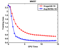
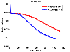
Figure 1 illustrates the convergence property of both Hogwild! and AsySVRG. The x-axis denotes the CPU time, where we set the CPU time that Hogwild! passes through the whole dataset once with one thread as 1 unit. The y-axis denotes the training loss. In this experiment, we run Hogwild! and AsySVRG with 10 threads. Hogwild!-10 and AsySVRG-10 denote the corresponding methods with 10 threads. It is easy to see that both Hogwild! and AsySVRG are convergent. Furthermore, AsySVRG is faster than Hogwild!. This is consistent with our theoretical results in this paper.
Refer to caption
(a) MNIST
Refer to caption
(b) connect-4
Figure 1: Hogwild! vs AsySVRG

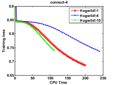
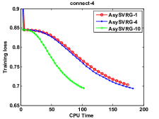
Figure 2 reports the results of Hogwild! and AsySVRG with different numbers of threads, where the number of threads p=1,4,10𝑝1410p=1,4,10. We can find that in most cases the two methods will become faster with the increase of threads. The only outlier is the case for Hogwild! on dateset connect-4, Hogwild! using 4 threads is slower than using 1 thread. One possible reason is that we have two CPUs in our server, with 6 cores for each CPU. In the 4-thread case, different threads may be allocated on different CPUs, which will cause extra cost.
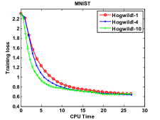
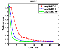
Refer to caption
(a) Hogwild! on MNIST
Refer to caption
(b) AsySVRG on MNIST
Refer to caption
(c) Hogwild! on connect-4
Refer to caption
(d) AsySVRG on connect-4
Figure 2: Comparison between different numbers of threads.

Conclusion

In this paper, we have provided theoretical proof about the convergence of two representative lock-free strategy based parallel SGD methods, Hogwild! and AsySVRG, for non-convex problems. Empirical results also show that both Hogwild! and AsySVRG are convergent on non-convex problems, which successfully verifies our theoretical results. To the best of our knowledge, this is the first work to prove the convergence of lock-free strategy based parallel SGD methods for non-convex problems.

Acknowledgements

This work is partially supported by NSFC (No. 61472182) and a fund from Tencent.

References

  • [Allen-Zhu and Hazan 2016] Allen-Zhu, Z., and Hazan, E. 2016. Variance reduction for faster non-convex optimization. In Proceedings of the 33nd International Conference on Machine Learning.
  • [Allen-Zhu and Yuan 2016] Allen-Zhu, Z., and Yuan, Y. 2016. Improved svrg for non-strongly-convex or sum-of-non-convex objectives. In Proceedings of the 33nd International Conference on Machine Learning.
  • [Chaturapruek, Duchi, and Ré 2015] Chaturapruek, S.; Duchi, J. C.; and Ré, C. 2015. Asynchronous stochastic convex optimization: the noise is in the noise and sgd don’t care. In Proceedings of the Advances in Neural Information Processing Systems.
  • [Ghadimi and Lan 2013] Ghadimi, S., and Lan, G. 2013. Stochastic first- and zeroth-order methods for nonconvex stochastic programming. SIAM Journal on Optimization 23(4):2341–2368.
  • [Huo and Huang 2016] Huo, Z., and Huang, H. 2016. Asynchronous stochastic gradient descent with variance reduction for non-convex optimization. CoRR abs/1604.03584.
  • [J. Reddi et al. 2015] J. Reddi, S.; Hefny, A.; Sra, S.; Poczos, B.; and Smola, A. J. 2015. On variance reduction in stochastic gradient descent and its asynchronous variants. In Proceedings of the Advances in Neural Information Processing Systems.
  • [Jaggi et al. 2014] Jaggi, M.; Smith, V.; Takac, M.; Terhorst, J.; Krishnan, S.; Hofmann, T.; and Jordan, M. I. 2014. Communication-efficient distributed dual coordinate ascent. In Proceedings of the Advances in Neural Information Processing Systems.
  • [Johnson and Zhang 2013] Johnson, R., and Zhang, T. 2013. Accelerating stochastic gradient descent using predictive variance reduction. In Proceedings of the Advances in Neural Information Processing Systems.
  • [Koren, Bell, and Volinsky 2009] Koren, Y.; Bell, R. M.; and Volinsky, C. 2009. Matrix factorization techniques for recommender systems. IEEE Computer 42(8):30–37.
  • [Krizhevsky, Sutskever, and Hinton 2012] Krizhevsky, A.; Sutskever, I.; and Hinton, G. E. 2012. Imagenet classification with deep convolutional neural networks. In Proceedings of the Advances in Neural Information Processing Systems.
  • [Li et al. 2014] Li, M.; Andersen, D. G.; Park, J. W.; Smola, A. J.; Ahmed, A.; Josifovski, V.; Long, J.; Shekita, E. J.; and Su, B. 2014. Scaling distributed machine learning with the parameter server. In Proceedings of the 11th USENIX Symposium on Operating Systems Design and Implementation.
  • [Li et al. 2016] Li, X.; Zhao, T.; Arora, R.; Han; and Haupt, J. 2016. Stochastic variance reduced optimization for nonconvex sparse learning. In Proceedings of the 33nd International Conference on Machine Learning.
  • [Lian et al. 2015] Lian, X.; Huang, Y.; Li, Y.; and Liu, J. 2015. Asynchronous parallel stochastic gradient for nonconvex optimization. In Proceedings of the Advances in Neural Information Processing Systems.
  • [Recht et al. 2011] Recht, B.; Re, C.; Wright, S.; and Niu, F. 2011. Hogwild!: A lock-free approach to parallelizing stochastic gradient descent. In Proceedings of the Advances in Neural Information Processing Systems.
  • [Reddi et al. 2016] Reddi, S. J.; Hefny, A.; Sra, S.; Poczos, B.; and Alex. 2016. Stochastic variance reduction for nonconvex optimization. In Proceedings of the 33nd International Conference on Machine Learning.
  • [Roux, Schmidt, and Bach 2012] Roux, N. L.; Schmidt, M. W.; and Bach, F. 2012. A stochastic gradient method with an exponential convergence rate for finite training sets. In Proceedings of the Advances in Neural Information Processing Systems.
  • [Sa, Re, and Olukotun 2015] Sa, C. D.; Re, C.; and Olukotun, K. 2015. Global convergence of stochastic gradient descent for some non-convex matrix problems. In Proceedings of the 32nd International Conference on Machine Learning.
  • [Shalev-Shwartz and Zhang 2013] Shalev-Shwartz, S., and Zhang, T. 2013. Stochastic dual coordinate ascent methods for regularized loss. Journal of Machine Learning Research 14(1):567–599.
  • [Shamir 2015] Shamir, O. 2015. A stochastic PCA and SVD algorithm with an exponential convergence rate. In Proceedings of the 32nd International Conference on Machine Learning.
  • [Shamir 2016a] Shamir, O. 2016a. Convergence of stochastic gradient descent for pca. In Proceedings of the 33nd International Conference on Machine Learning.
  • [Shamir 2016b] Shamir, O. 2016b. Fast stochastic algorithms for svd and pca: Convergence properties and convexity. In Proceedings of the 33nd International Conference on Machine Learning.
  • [Xing et al. 2015] Xing, E. P.; Ho, Q.; Dai, W.; Kim, J. K.; Wei, J.; Lee, S.; Zheng, X.; Xie, P.; Kumar, A.; and Yu, Y. 2015. Petuum: A new platform for distributed machine learning on big data. In Proceedings of the 21th ACM SIGKDD International Conference on Knowledge Discovery and Data Mining.
  • [Zhang, Zheng, and Kwok 2016] Zhang, R.; Zheng, S.; and Kwok, J. T. 2016. Asynchronous distributed semi-stochastic gradient optimization. In Proceedings of the AAAI Conference on Artificial Intelligence.
  • [Zhao and Li 2016] Zhao, S.-Y., and Li, W.-J. 2016. Fast asynchronous parallel stochastic gradient descent: A lock-free approach with convergence guarantee. In Proceedings of the AAAI Conference on Artificial Intelligence.

Appendix A Appendix

Proof of Lemma 2

Proof.

First, 𝐱,𝐲for-all𝐱𝐲\forall{\bf x},{\bf y} and r>0𝑟0r>0, we have:

fi(𝐱)2fi(𝐲)2superscriptnormsubscript𝑓𝑖𝐱2superscriptnormsubscript𝑓𝑖𝐲2\displaystyle\left\|\nabla f_{i}({\bf x})\right\|^{2}-\left\|\nabla f_{i}({\bf y})\right\|^{2}
\displaystyle\leq 2fi(𝐱)T(fi(𝐱)fi(𝐲))2subscript𝑓𝑖superscript𝐱𝑇subscript𝑓𝑖𝐱subscript𝑓𝑖𝐲\displaystyle 2\nabla f_{i}({\bf x})^{T}(\nabla f_{i}({\bf x})-\nabla f_{i}({\bf y}))
\displaystyle\leq 1rfi(𝐱)2+rfi(𝐱)fi(𝐲)21𝑟superscriptnormsubscript𝑓𝑖𝐱2𝑟superscriptnormsubscript𝑓𝑖𝐱subscript𝑓𝑖𝐲2\displaystyle\frac{1}{r}\left\|\nabla f_{i}({\bf x})\right\|^{2}+r\left\|\nabla f_{i}({\bf x})-\nabla f_{i}({\bf y})\right\|^{2}
=\displaystyle= 1rfi(𝐱)2+rfi(𝐱)fi(𝐲)21𝑟superscriptnormsubscript𝑓𝑖𝐱2𝑟superscriptnormsubscript𝑓𝑖𝐱subscript𝑓𝑖𝐲2\displaystyle\frac{1}{r}\left\|\nabla f_{i}({\bf x})\right\|^{2}+r\left\|\nabla f_{i}({\bf x})-\nabla f_{i}({\bf y})\right\|^{2}
\displaystyle\leq 1rfi(𝐱)2+rL2𝐱𝐲21𝑟superscriptnormsubscript𝑓𝑖𝐱2𝑟superscript𝐿2superscriptnorm𝐱𝐲2\displaystyle\frac{1}{r}\left\|\nabla f_{i}({\bf x})\right\|^{2}+rL^{2}\left\|{\bf x}-{\bf y}\right\|^{2} (10)

In the above equation, take 𝐱=𝐰^t,𝐲=𝐰^t+1formulae-sequence𝐱subscript^𝐰𝑡𝐲subscript^𝐰𝑡1{\bf x}=\hat{{\bf w}}_{t},{\bf y}=\hat{{\bf w}}_{t+1}, we obtain:

fi(𝐰^t)2fi(𝐰^t+1)2superscriptnormsubscript𝑓𝑖subscript^𝐰𝑡2superscriptnormsubscript𝑓𝑖subscript^𝐰𝑡12\displaystyle\left\|\nabla f_{i}(\hat{{\bf w}}_{t})\right\|^{2}-\left\|\nabla f_{i}(\hat{{\bf w}}_{t+1})\right\|^{2}
\displaystyle\leq 1rfi(𝐰^t)2+rL2𝐰^t𝐰^t+121𝑟superscriptnormsubscript𝑓𝑖subscript^𝐰𝑡2𝑟superscript𝐿2superscriptnormsubscript^𝐰𝑡subscript^𝐰𝑡12\displaystyle\frac{1}{r}\left\|\nabla f_{i}(\hat{{\bf w}}_{t})\right\|^{2}+rL^{2}\left\|\hat{{\bf w}}_{t}-\hat{{\bf w}}_{t+1}\right\|^{2}

According to the definition of 𝐰^tsubscript^𝐰𝑡\hat{{\bf w}}_{t}, we have

𝐰^t𝐰^t+1normsubscript^𝐰𝑡subscript^𝐰𝑡1\displaystyle\left\|\hat{{\bf w}}_{t}-\hat{{\bf w}}_{t+1}\right\|
=\displaystyle= 𝐰a(t)ηj=a(t)t1𝐏t,ja(t)fij(𝐰^j)\displaystyle\|{\bf w}_{a(t)}-\eta\sum_{j=a(t)}^{t-1}{\bf P}_{t,j-a(t)}\nabla f_{i_{j}}(\hat{{\bf w}}_{j})
(𝐰a(t+1)ηj=a(t+1)t𝐏t+1,ja(t+1)fij(𝐰^j))\displaystyle-({\bf w}_{a(t+1)}-\eta\sum_{j=a(t+1)}^{t}{\bf P}_{t+1,j-a(t+1)}\nabla f_{i_{j}}(\hat{{\bf w}}_{j}))\|
\displaystyle\leq 𝐰a(t)𝐰a(t+1)normsubscript𝐰𝑎𝑡subscript𝐰𝑎𝑡1\displaystyle\left\|{\bf w}_{a(t)}-{\bf w}_{a(t+1)}\right\|
+ηj=a(t)t1fij(𝐰^j)+ηj=a(t+1)tfij(𝐰^j)𝜂superscriptsubscript𝑗𝑎𝑡𝑡1normsubscript𝑓subscript𝑖𝑗subscript^𝐰𝑗𝜂superscriptsubscript𝑗𝑎𝑡1𝑡normsubscript𝑓subscript𝑖𝑗subscript^𝐰𝑗\displaystyle+\eta\sum_{j=a(t)}^{t-1}\left\|\nabla f_{i_{j}}(\hat{{\bf w}}_{j})\right\|+\eta\sum_{j=a(t+1)}^{t}\left\|\nabla f_{i_{j}}(\hat{{\bf w}}_{j})\right\|
\displaystyle\leq j=a(t)a(t+1)1𝐰j𝐰j+1superscriptsubscript𝑗𝑎𝑡𝑎𝑡11normsubscript𝐰𝑗subscript𝐰𝑗1\displaystyle\sum_{j=a(t)}^{a(t+1)-1}\left\|{\bf w}_{j}-{\bf w}_{j+1}\right\|
+ηj=a(t)t1fij(𝐰^j)+ηj=a(t+1)tfij(𝐰^j)𝜂superscriptsubscript𝑗𝑎𝑡𝑡1normsubscript𝑓subscript𝑖𝑗subscript^𝐰𝑗𝜂superscriptsubscript𝑗𝑎𝑡1𝑡normsubscript𝑓subscript𝑖𝑗subscript^𝐰𝑗\displaystyle+\eta\sum_{j=a(t)}^{t-1}\left\|\nabla f_{i_{j}}(\hat{{\bf w}}_{j})\right\|+\eta\sum_{j=a(t+1)}^{t}\left\|\nabla f_{i_{j}}(\hat{{\bf w}}_{j})\right\|
\displaystyle\leq ηj=a(t)a(t+1)1fij(𝐰^j)𝜂superscriptsubscript𝑗𝑎𝑡𝑎𝑡11normsubscript𝑓subscript𝑖𝑗subscript^𝐰𝑗\displaystyle\eta\sum_{j=a(t)}^{a(t+1)-1}\left\|\nabla f_{i_{j}}(\hat{{\bf w}}_{j})\right\|
+ηj=a(t)t1fij(𝐰^j)+ηj=a(t+1)tfij(𝐰^j)𝜂superscriptsubscript𝑗𝑎𝑡𝑡1normsubscript𝑓subscript𝑖𝑗subscript^𝐰𝑗𝜂superscriptsubscript𝑗𝑎𝑡1𝑡normsubscript𝑓subscript𝑖𝑗subscript^𝐰𝑗\displaystyle+\eta\sum_{j=a(t)}^{t-1}\left\|\nabla f_{i_{j}}(\hat{{\bf w}}_{j})\right\|+\eta\sum_{j=a(t+1)}^{t}\left\|\nabla f_{i_{j}}(\hat{{\bf w}}_{j})\right\|
\displaystyle\leq 3ηj=tτtfij(𝐰^j).3𝜂superscriptsubscript𝑗𝑡𝜏𝑡normsubscript𝑓subscript𝑖𝑗subscript^𝐰𝑗\displaystyle 3\eta\sum_{j=t-\tau}^{t}\left\|\nabla f_{i_{j}}(\hat{{\bf w}}_{j})\right\|.

Combining the two above equation, we obtain:

fi(𝐰^t)2fi(𝐰^t+1)2superscriptnormsubscript𝑓𝑖subscript^𝐰𝑡2superscriptnormsubscript𝑓𝑖subscript^𝐰𝑡12\displaystyle\left\|\nabla f_{i}(\hat{{\bf w}}_{t})\right\|^{2}-\left\|\nabla f_{i}(\hat{{\bf w}}_{t+1})\right\|^{2}
\displaystyle\leq 1rfi(𝐰^t)2+9r(τ+1)L2η2j=tτtfij(𝐰^j)21𝑟superscriptnormsubscript𝑓𝑖subscript^𝐰𝑡29𝑟𝜏1superscript𝐿2superscript𝜂2superscriptsubscript𝑗𝑡𝜏𝑡superscriptnormsubscript𝑓subscript𝑖𝑗subscript^𝐰𝑗2\displaystyle\frac{1}{r}\left\|\nabla f_{i}(\hat{{\bf w}}_{t})\right\|^{2}+9r(\tau+1)L^{2}\eta^{2}\sum_{j=t-\tau}^{t}\left\|\nabla f_{i_{j}}(\hat{{\bf w}}_{j})\right\|^{2}

For any fixed i𝑖i, we take expectation on the random index ijsubscript𝑖𝑗i_{j}, we obtain:

fi(𝐰^t)2fi(𝐰^t+1)2superscriptnormsubscript𝑓𝑖subscript^𝐰𝑡2superscriptnormsubscript𝑓𝑖subscript^𝐰𝑡12\displaystyle\left\|\nabla f_{i}(\hat{{\bf w}}_{t})\right\|^{2}-\left\|\nabla f_{i}(\hat{{\bf w}}_{t+1})\right\|^{2}
\displaystyle\leq 1rfi(𝐰^t)2+9r(τ+1)L2η2j=tτtq(𝐰^j)1𝑟superscriptnormsubscript𝑓𝑖subscript^𝐰𝑡29𝑟𝜏1superscript𝐿2superscript𝜂2superscriptsubscript𝑗𝑡𝜏𝑡𝑞subscript^𝐰𝑗\displaystyle\frac{1}{r}\left\|\nabla f_{i}(\hat{{\bf w}}_{t})\right\|^{2}+9r(\tau+1)L^{2}\eta^{2}\sum_{j=t-\tau}^{t}q(\hat{{\bf w}}_{j})

Summing up i𝑖i from 111 to n𝑛n, we obtain:

𝔼q(𝐰^t)𝔼q(𝐰^t+1)𝔼𝑞subscript^𝐰𝑡𝔼𝑞subscript^𝐰𝑡1\displaystyle{\mathbb{E}}q(\hat{{\bf w}}_{t})-{\mathbb{E}}q(\hat{{\bf w}}_{t+1})
\displaystyle\leq 1r𝔼q(𝐰^t)+9r(τ+1)L2η2j=tτt𝔼q(𝐰^j)1𝑟𝔼𝑞subscript^𝐰𝑡9𝑟𝜏1superscript𝐿2superscript𝜂2superscriptsubscript𝑗𝑡𝜏𝑡𝔼𝑞subscript^𝐰𝑗\displaystyle\frac{1}{r}{\mathbb{E}}q(\hat{{\bf w}}_{t})+9r(\tau+1)L^{2}\eta^{2}\sum_{j=t-\tau}^{t}{\mathbb{E}}q(\hat{{\bf w}}_{j})

Now, we prove the final result by induction and take r=1η𝑟1𝜂r=\frac{1}{\eta}. When t=0𝑡0t=0, we have

𝔼q(𝐰^0)11η9η(τ+1)L2𝔼q(𝐰^1)ρ𝔼q(𝐰^1)𝔼𝑞subscript^𝐰011𝜂9𝜂𝜏1superscript𝐿2𝔼𝑞subscript^𝐰1𝜌𝔼𝑞subscript^𝐰1\displaystyle{\mathbb{E}}q(\hat{{\bf w}}_{0})\leq\frac{1}{1-\eta-9\eta(\tau+1)L^{2}}{\mathbb{E}}q(\hat{{\bf w}}_{1})\leq\rho{\mathbb{E}}q(\hat{{\bf w}}_{1})

Assuming the result is right for t1𝑡1t-1, then we have

𝔼q(𝐰^t)𝔼q(𝐰^t+1)𝔼𝑞subscript^𝐰𝑡𝔼𝑞subscript^𝐰𝑡1\displaystyle{\mathbb{E}}q(\hat{{\bf w}}_{t})-{\mathbb{E}}q(\hat{{\bf w}}_{t+1})
\displaystyle\leq 1r𝔼q(𝐰^t)+9η(τ+1)L2𝔼q(𝐰^j)j=tτtρtj1𝑟𝔼𝑞subscript^𝐰𝑡9𝜂𝜏1superscript𝐿2𝔼𝑞subscript^𝐰𝑗superscriptsubscript𝑗𝑡𝜏𝑡superscript𝜌𝑡𝑗\displaystyle\frac{1}{r}{\mathbb{E}}q(\hat{{\bf w}}_{t})+9\eta(\tau+1)L^{2}{\mathbb{E}}q(\hat{{\bf w}}_{j})\sum_{j=t-\tau}^{t}\rho^{t-j}

which means

𝔼q(𝐰^t)11η9η(τ+1)L2(ρτ+11)ρ1𝔼q(𝐰^t+1)ρ𝔼q(𝐰^t+1)𝔼𝑞subscript^𝐰𝑡11𝜂9𝜂𝜏1superscript𝐿2superscript𝜌𝜏11𝜌1𝔼𝑞subscript^𝐰𝑡1𝜌𝔼𝑞subscript^𝐰𝑡1\displaystyle{\mathbb{E}}q(\hat{{\bf w}}_{t})\leq\frac{1}{1-\eta-\frac{9\eta(\tau+1)L^{2}(\rho^{\tau+1}-1)}{\rho-1}}{\mathbb{E}}q(\hat{{\bf w}}_{t+1})\leq\rho{\mathbb{E}}q(\hat{{\bf w}}_{t+1})

Proof of Lemma 3

Proof.
𝐰t𝐰^tnormsubscript𝐰𝑡subscript^𝐰𝑡\displaystyle\|{\bf w}_{t}-\hat{{\bf w}}_{t}\|
=\displaystyle= 𝐰t𝐰a(t)+ηj=a(t)t1𝐏t,ja(t)fij(𝐰^j)normsubscript𝐰𝑡subscript𝐰𝑎𝑡𝜂superscriptsubscript𝑗𝑎𝑡𝑡1subscript𝐏𝑡𝑗𝑎𝑡subscript𝑓subscript𝑖𝑗subscript^𝐰𝑗\displaystyle\|{\bf w}_{t}-{\bf w}_{a(t)}+\eta\sum_{j=a(t)}^{t-1}{\bf P}_{t,j-a(t)}\nabla f_{i_{j}}(\hat{{\bf w}}_{j})\|
\displaystyle\leq 𝐰t𝐰a(t)+ηj=a(t)t1fij(𝐰^j)normsubscript𝐰𝑡subscript𝐰𝑎𝑡𝜂superscriptsubscript𝑗𝑎𝑡𝑡1normsubscript𝑓subscript𝑖𝑗subscript^𝐰𝑗\displaystyle\|{\bf w}_{t}-{\bf w}_{a(t)}\|+\eta\sum_{j=a(t)}^{t-1}\|\nabla f_{i_{j}}(\hat{{\bf w}}_{j})\|
\displaystyle\leq j=a(t)t1𝐰j𝐰j+1+ηj=a(t)t1fij(𝐰^j)superscriptsubscript𝑗𝑎𝑡𝑡1normsubscript𝐰𝑗subscript𝐰𝑗1𝜂superscriptsubscript𝑗𝑎𝑡𝑡1normsubscript𝑓subscript𝑖𝑗subscript^𝐰𝑗\displaystyle\sum_{j=a(t)}^{t-1}\|{\bf w}_{j}-{\bf w}_{j+1}\|+\eta\sum_{j=a(t)}^{t-1}\|\nabla f_{i_{j}}(\hat{{\bf w}}_{j})\|
\displaystyle\leq 2ηj=a(t)t1fij(𝐰^j)2𝜂superscriptsubscript𝑗𝑎𝑡𝑡1normsubscript𝑓subscript𝑖𝑗subscript^𝐰𝑗\displaystyle 2\eta\sum_{j=a(t)}^{t-1}\|\nabla f_{i_{j}}(\hat{{\bf w}}_{j})\|

Then we get the result

𝔼𝐰t𝐰^t2𝔼superscriptnormsubscript𝐰𝑡subscript^𝐰𝑡2absent\displaystyle{\mathbb{E}}\|{\bf w}_{t}-\hat{{\bf w}}_{t}\|^{2}\leq 4η2τj=a(t)t1𝔼fij(𝐰^j)24superscript𝜂2𝜏superscriptsubscript𝑗𝑎𝑡𝑡1𝔼superscriptnormsubscript𝑓subscript𝑖𝑗subscript^𝐰𝑗2\displaystyle 4\eta^{2}\tau\sum_{j=a(t)}^{t-1}{\mathbb{E}}\|\nabla f_{i_{j}}(\hat{{\bf w}}_{j})\|^{2}
=\displaystyle= 4η2τj=a(t)t1𝔼q(𝐰^j)4superscript𝜂2𝜏superscriptsubscript𝑗𝑎𝑡𝑡1𝔼𝑞subscript^𝐰𝑗\displaystyle 4\eta^{2}\tau\sum_{j=a(t)}^{t-1}{\mathbb{E}}q(\hat{{\bf w}}_{j})
\displaystyle\leq 4η2τρ(ρτ1)ρ1𝔼q(𝐰^t)4superscript𝜂2𝜏𝜌superscript𝜌𝜏1𝜌1𝔼𝑞subscript^𝐰𝑡\displaystyle\frac{4\eta^{2}\tau\rho(\rho^{\tau}-1)}{\rho-1}{\mathbb{E}}q(\hat{{\bf w}}_{t})

where the last inequality uses Lemma 2 in the appendix. ∎

Proof of Lemma 5

Proof.

First, 𝐱,𝐲for-all𝐱𝐲\forall{\bf x},{\bf y} and r>0𝑟0r>0, we have:

𝐩i(𝐱)2𝐩i(𝐲)2superscriptnormsubscript𝐩𝑖𝐱2superscriptnormsubscript𝐩𝑖𝐲2\displaystyle\left\|{\bf p}_{i}({\bf x})\right\|^{2}-\left\|{\bf p}_{i}({\bf y})\right\|^{2}
\displaystyle\leq 2𝐩i(𝐱)T(𝐩i(𝐱)𝐩i(𝐲))2subscript𝐩𝑖superscript𝐱𝑇subscript𝐩𝑖𝐱subscript𝐩𝑖𝐲\displaystyle 2{\bf p}_{i}({\bf x})^{T}({\bf p}_{i}({\bf x})-{\bf p}_{i}({\bf y}))
\displaystyle\leq 1r𝐩i(𝐱)2+r𝐩i(𝐱)𝐩i(𝐲)21𝑟superscriptnormsubscript𝐩𝑖𝐱2𝑟superscriptnormsubscript𝐩𝑖𝐱subscript𝐩𝑖𝐲2\displaystyle\frac{1}{r}\left\|{\bf p}_{i}({\bf x})\right\|^{2}+r\left\|{\bf p}_{i}({\bf x})-{\bf p}_{i}({\bf y})\right\|^{2}
=\displaystyle= 1r𝐩i(𝐱)2+r𝐩i(𝐱)𝐩i(𝐲)21𝑟superscriptnormsubscript𝐩𝑖𝐱2𝑟superscriptnormsubscript𝐩𝑖𝐱subscript𝐩𝑖𝐲2\displaystyle\frac{1}{r}\left\|{\bf p}_{i}({\bf x})\right\|^{2}+r\left\|{\bf p}_{i}({\bf x})-{\bf p}_{i}({\bf y})\right\|^{2}
\displaystyle\leq 1r𝐩i(𝐱)2+rL2𝐱𝐲21𝑟superscriptnormsubscript𝐩𝑖𝐱2𝑟superscript𝐿2superscriptnorm𝐱𝐲2\displaystyle\frac{1}{r}\left\|{\bf p}_{i}({\bf x})\right\|^{2}+rL^{2}\left\|{\bf x}-{\bf y}\right\|^{2} (11)

In the above equation, take 𝐱=𝐮^t,m,𝐲=𝐮^t,m+1formulae-sequence𝐱subscript^𝐮𝑡𝑚𝐲subscript^𝐮𝑡𝑚1{\bf x}=\hat{{\bf u}}_{t,m},{\bf y}=\hat{{\bf u}}_{t,m+1}, we obtain:

𝐩i(𝐮^t,m)2𝐩i(𝐮^t,m+1)2superscriptnormsubscript𝐩𝑖subscript^𝐮𝑡𝑚2superscriptnormsubscript𝐩𝑖subscript^𝐮𝑡𝑚12\displaystyle\left\|{\bf p}_{i}(\hat{{\bf u}}_{t,m})\right\|^{2}-\left\|{\bf p}_{i}(\hat{{\bf u}}_{t,m+1})\right\|^{2}
\displaystyle\leq 1r𝐩i(𝐮^t,m)2+rL2𝐮^t,m𝐮^t,m+121𝑟superscriptnormsubscript𝐩𝑖subscript^𝐮𝑡𝑚2𝑟superscript𝐿2superscriptnormsubscript^𝐮𝑡𝑚subscript^𝐮𝑡𝑚12\displaystyle\frac{1}{r}\left\|{\bf p}_{i}(\hat{{\bf u}}_{t,m})\right\|^{2}+rL^{2}\left\|\hat{{\bf u}}_{t,m}-\hat{{\bf u}}_{t,m+1}\right\|^{2}

Furthermore, we can get

𝐮^t,m𝐮^t,m+1normsubscript^𝐮𝑡𝑚subscript^𝐮𝑡𝑚1\displaystyle\left\|\hat{{\bf u}}_{t,m}-\hat{{\bf u}}_{t,m+1}\right\|
=\displaystyle= 𝐮t,a(m)ηi=a(m)m1𝐏m,ia(m)(t)𝐯^t,i\displaystyle\|{\bf u}_{t,a(m)}-\eta\sum_{i=a(m)}^{m-1}{\bf P}_{m,i-a(m)}^{(t)}\hat{{\bf v}}_{t,i}
(𝐮t,a(m+1)ηi=a(m+1)m𝐏m+1,ia(m+1)(t)𝐯^t,i)\displaystyle-({\bf u}_{t,a(m+1)}-\eta\sum_{i=a(m+1)}^{m}{\bf P}_{m+1,i-a(m+1)}^{(t)}\hat{{\bf v}}_{t,i})\|
\displaystyle\leq 𝐮t,a(m)𝐮t,a(m+1)+ηi=a(m)m1𝐯^t,i+ηi=a(m+1)m𝐯^t,inormsubscript𝐮𝑡𝑎𝑚subscript𝐮𝑡𝑎𝑚1𝜂superscriptsubscript𝑖𝑎𝑚𝑚1normsubscript^𝐯𝑡𝑖𝜂superscriptsubscript𝑖𝑎𝑚1𝑚normsubscript^𝐯𝑡𝑖\displaystyle\left\|{\bf u}_{t,a(m)}-{\bf u}_{t,a(m+1)}\right\|+\eta\sum_{i=a(m)}^{m-1}\left\|\hat{{\bf v}}_{t,i}\right\|+\eta\sum_{i=a(m+1)}^{m}\left\|\hat{{\bf v}}_{t,i}\right\|
\displaystyle\leq i=a(m)a(m+1)1𝐮t,i𝐮t,i+1+ηi=a(m)m1𝐯^t,i+ηi=a(m+1)m𝐯^t,isuperscriptsubscript𝑖𝑎𝑚𝑎𝑚11normsubscript𝐮𝑡𝑖subscript𝐮𝑡𝑖1𝜂superscriptsubscript𝑖𝑎𝑚𝑚1normsubscript^𝐯𝑡𝑖𝜂superscriptsubscript𝑖𝑎𝑚1𝑚normsubscript^𝐯𝑡𝑖\displaystyle\sum_{i=a(m)}^{a(m+1)-1}\left\|{\bf u}_{t,i}-{\bf u}_{t,i+1}\right\|+\eta\sum_{i=a(m)}^{m-1}\left\|\hat{{\bf v}}_{t,i}\right\|+\eta\sum_{i=a(m+1)}^{m}\left\|\hat{{\bf v}}_{t,i}\right\|
\displaystyle\leq ηi=a(m)a(m+1)1𝐯^t,i+ηi=a(m)m1𝐯^t,i+ηi=a(m+1)m𝐯^t,i𝜂superscriptsubscript𝑖𝑎𝑚𝑎𝑚11normsubscript^𝐯𝑡𝑖𝜂superscriptsubscript𝑖𝑎𝑚𝑚1normsubscript^𝐯𝑡𝑖𝜂superscriptsubscript𝑖𝑎𝑚1𝑚normsubscript^𝐯𝑡𝑖\displaystyle\eta\sum_{i=a(m)}^{a(m+1)-1}\left\|\hat{{\bf v}}_{t,i}\right\|+\eta\sum_{i=a(m)}^{m-1}\left\|\hat{{\bf v}}_{t,i}\right\|+\eta\sum_{i=a(m+1)}^{m}\left\|\hat{{\bf v}}_{t,i}\right\|
\displaystyle\leq 3ηi=mτm𝐯^t,i.3𝜂superscriptsubscript𝑖𝑚𝜏𝑚normsubscript^𝐯𝑡𝑖\displaystyle 3\eta\sum_{i=m-\tau}^{m}\left\|\hat{{\bf v}}_{t,i}\right\|.

Then, we take r=1η𝑟1𝜂r=\frac{1}{\eta} have

𝐩i(𝐮^t,m)2𝐩i(𝐮^t,m+1)2superscriptnormsubscript𝐩𝑖subscript^𝐮𝑡𝑚2superscriptnormsubscript𝐩𝑖subscript^𝐮𝑡𝑚12\displaystyle\left\|{\bf p}_{i}(\hat{{\bf u}}_{t,m})\right\|^{2}-\left\|{\bf p}_{i}(\hat{{\bf u}}_{t,m+1})\right\|^{2}
\displaystyle\leq η𝐩i(𝐮^t,m)2+9η(τ+1)L2j=mτm𝐯^t,j2𝜂superscriptnormsubscript𝐩𝑖subscript^𝐮𝑡𝑚29𝜂𝜏1superscript𝐿2superscriptsubscript𝑗𝑚𝜏𝑚superscriptnormsubscript^𝐯𝑡𝑗2\displaystyle\eta\left\|{\bf p}_{i}(\hat{{\bf u}}_{t,m})\right\|^{2}+9\eta(\tau+1)L^{2}\sum_{j=m-\tau}^{m}\left\|\hat{{\bf v}}_{t,j}\right\|^{2}

For any fixed i𝑖i, we can take expectation for both sides of the above inequality and then sum i𝑖i from 111 to n𝑛n. Then we can get:

𝔼q(𝐮^t,m)𝔼q(𝐮^t,m+1)𝔼𝑞subscript^𝐮𝑡𝑚𝔼𝑞subscript^𝐮𝑡𝑚1\displaystyle{\mathbb{E}}q(\hat{{\bf u}}_{t,m})-{\mathbb{E}}q(\hat{{\bf u}}_{t,m+1})
\displaystyle\leq η𝔼q(𝐮^t,m)+9η(τ+1)L2j=mτm𝔼q(𝐮^t,j)𝜂𝔼𝑞subscript^𝐮𝑡𝑚9𝜂𝜏1superscript𝐿2superscriptsubscript𝑗𝑚𝜏𝑚𝔼𝑞subscript^𝐮𝑡𝑗\displaystyle\eta{\mathbb{E}}q(\hat{{\bf u}}_{t,m})+9\eta(\tau+1)L^{2}\sum_{j=m-\tau}^{m}{\mathbb{E}}q(\hat{{\bf u}}_{t,j})

Here we use the fact that 𝔼[𝐯^t,j2|𝐮^t,j]=q(𝐮^t,j)𝔼delimited-[]conditionalsuperscriptnormsubscript^𝐯𝑡𝑗2subscript^𝐮𝑡𝑗𝑞subscript^𝐮𝑡𝑗{\mathbb{E}}[\|\hat{{\bf v}}_{t,j}\|^{2}|\hat{{\bf u}}_{t,j}]=q(\hat{{\bf u}}_{t,j}).

We prove our conclusion by induction. For convenience, we use qisubscript𝑞𝑖q_{i} to denote 𝔼q(𝐮^t,i)𝔼𝑞subscript^𝐮𝑡𝑖{\mathbb{E}}q(\hat{{\bf u}}_{t,i}).

When m=0𝑚0m=0, we have

q011η9η(τ+1)L2q1ρq1subscript𝑞011𝜂9𝜂𝜏1superscript𝐿2subscript𝑞1𝜌subscript𝑞1\displaystyle q_{0}\leq\frac{1}{1-\eta-9\eta(\tau+1)L^{2}}q_{1}\leq\rho q_{1}

Assuming that mM0for-all𝑚subscript𝑀0\forall m\leq M_{0}, we have qm1ρqmsubscript𝑞𝑚1𝜌subscript𝑞𝑚q_{m-1}\leq\rho q_{m}, then for m=M0𝑚subscript𝑀0m=M_{0}, we have

qmlimit-fromsubscript𝑞𝑚\displaystyle q_{m}- qm+1ηqm+9η(τ+1)L2j=mτmqjsubscript𝑞𝑚1𝜂subscript𝑞𝑚9𝜂𝜏1superscript𝐿2superscriptsubscript𝑗𝑚𝜏𝑚subscript𝑞𝑗\displaystyle q_{m+1}\leq\eta q_{m}+9\eta(\tau+1)L^{2}\sum_{j=m-\tau}^{m}q_{j}
\displaystyle\leq ηqm+9η(τ+1)L2qmj=mτmρmj𝜂subscript𝑞𝑚9𝜂𝜏1superscript𝐿2subscript𝑞𝑚superscriptsubscript𝑗𝑚𝜏𝑚superscript𝜌𝑚𝑗\displaystyle\eta q_{m}+9\eta(\tau+1)L^{2}q_{m}\sum_{j=m-\tau}^{m}\rho^{m-j}
=\displaystyle= ηqm+9η(τ+1)L2(ρτ+11)ρ1qm𝜂subscript𝑞𝑚9𝜂𝜏1superscript𝐿2superscript𝜌𝜏11𝜌1subscript𝑞𝑚\displaystyle\eta q_{m}+\frac{9\eta(\tau+1)L^{2}(\rho^{\tau+1}-1)}{\rho-1}q_{m}

which means that

qm11η9η(τ+1)L2(ρτ+11)ρ1qm+1ρqm+1subscript𝑞𝑚11𝜂9𝜂𝜏1superscript𝐿2superscript𝜌𝜏11𝜌1subscript𝑞𝑚1𝜌subscript𝑞𝑚1\displaystyle q_{m}\leq\frac{1}{1-\eta-\frac{9\eta(\tau+1)L^{2}(\rho^{\tau+1}-1)}{\rho-1}}q_{m+1}\leq\rho q_{m+1}

Proof of Lemma 6

Proof.
𝐮^t,m𝐮t,mnormsubscript^𝐮𝑡𝑚subscript𝐮𝑡𝑚\displaystyle\left\|\hat{{\bf u}}_{t,m}-{\bf u}_{t,m}\right\|
=\displaystyle= 𝐮t,a(m)ηj=a(m)m1𝐏m,ja(m)(t)𝐯^t,j𝐮t,mnormsubscript𝐮𝑡𝑎𝑚𝜂superscriptsubscript𝑗𝑎𝑚𝑚1superscriptsubscript𝐏𝑚𝑗𝑎𝑚𝑡subscript^𝐯𝑡𝑗subscript𝐮𝑡𝑚\displaystyle\left\|{\bf u}_{t,a(m)}-\eta\sum_{j=a(m)}^{m-1}{\bf P}_{m,j-a(m)}^{(t)}\hat{{\bf v}}_{t,j}-{\bf u}_{t,m}\right\|
\displaystyle\leq 𝐮t,a(m)𝐮t,m+ηj=a(m)m1𝐯^t,jnormsubscript𝐮𝑡𝑎𝑚subscript𝐮𝑡𝑚𝜂superscriptsubscript𝑗𝑎𝑚𝑚1normsubscript^𝐯𝑡𝑗\displaystyle\left\|{\bf u}_{t,a(m)}-{\bf u}_{t,m}\right\|+\eta\sum_{j=a(m)}^{m-1}\left\|\hat{{\bf v}}_{t,j}\right\|
\displaystyle\leq j=a(m)m1𝐮t,j𝐮t,j+1+ηj=a(m)m1𝐯^t,jsuperscriptsubscript𝑗𝑎𝑚𝑚1normsubscript𝐮𝑡𝑗subscript𝐮𝑡𝑗1𝜂superscriptsubscript𝑗𝑎𝑚𝑚1normsubscript^𝐯𝑡𝑗\displaystyle\sum_{j=a(m)}^{m-1}\left\|{\bf u}_{t,j}-{\bf u}_{t,j+1}\right\|+\eta\sum_{j=a(m)}^{m-1}\left\|\hat{{\bf v}}_{t,j}\right\|
\displaystyle\leq ηj=a(m)m1𝐯^t,j+ηj=a(m)m1𝐯^t,j𝜂superscriptsubscript𝑗𝑎𝑚𝑚1normsubscript^𝐯𝑡𝑗𝜂superscriptsubscript𝑗𝑎𝑚𝑚1normsubscript^𝐯𝑡𝑗\displaystyle\eta\sum_{j=a(m)}^{m-1}\left\|\hat{{\bf v}}_{t,j}\right\|+\eta\sum_{j=a(m)}^{m-1}\left\|\hat{{\bf v}}_{t,j}\right\|
\displaystyle\leq 2ηj=a(m)m1𝐯^t,j2𝜂superscriptsubscript𝑗𝑎𝑚𝑚1normsubscript^𝐯𝑡𝑗\displaystyle 2\eta\sum_{j=a(m)}^{m-1}\left\|\hat{{\bf v}}_{t,j}\right\| (12)

Then we get the result

𝔼𝐮^t,m𝐮t,m2𝔼superscriptnormsubscript^𝐮𝑡𝑚subscript𝐮𝑡𝑚2absent\displaystyle{\mathbb{E}}\left\|\hat{{\bf u}}_{t,m}-{\bf u}_{t,m}\right\|^{2}\leq 4η2τj=a(m)m1𝔼𝐯^t,j24superscript𝜂2𝜏superscriptsubscript𝑗𝑎𝑚𝑚1𝔼superscriptnormsubscript^𝐯𝑡𝑗2\displaystyle 4\eta^{2}\tau\sum_{j=a(m)}^{m-1}{\mathbb{E}}\left\|\hat{{\bf v}}_{t,j}\right\|^{2}
=\displaystyle= 4η2τj=a(m)m1𝔼q(𝐮^t,j)4superscript𝜂2𝜏superscriptsubscript𝑗𝑎𝑚𝑚1𝔼𝑞subscript^𝐮𝑡𝑗\displaystyle 4\eta^{2}\tau\sum_{j=a(m)}^{m-1}{\mathbb{E}}q(\hat{{\bf u}}_{t,j})
\displaystyle\leq 4η2τρ(ρτ1)ρ1𝔼q(𝐮^t,m)4superscript𝜂2𝜏𝜌superscript𝜌𝜏1𝜌1𝔼𝑞subscript^𝐮𝑡𝑚\displaystyle\frac{4\eta^{2}\tau\rho(\rho^{\tau}-1)}{\rho-1}{\mathbb{E}}q(\hat{{\bf u}}_{t,m})

where the last inequality uses Lemma 5. ∎

Proof of Lemma 7

Proof.

First, for any fixed i𝑖i, we have

𝐩i(𝐮^t,m)2𝐩i(𝐮t,m)2superscriptnormsubscript𝐩𝑖subscript^𝐮𝑡𝑚2superscriptnormsubscript𝐩𝑖subscript𝐮𝑡𝑚2\displaystyle\left\|{\bf p}_{i}(\hat{{\bf u}}_{t,m})\right\|^{2}-\left\|{\bf p}_{i}({\bf u}_{t,m})\right\|^{2}
\displaystyle\leq 2𝐩i(𝐱)T(𝐩i(𝐮^t,m)𝐩i(𝐮t,m))2subscript𝐩𝑖superscript𝐱𝑇subscript𝐩𝑖subscript^𝐮𝑡𝑚subscript𝐩𝑖subscript𝐮𝑡𝑚\displaystyle 2{\bf p}_{i}({\bf x})^{T}({\bf p}_{i}(\hat{{\bf u}}_{t,m})-{\bf p}_{i}({\bf u}_{t,m}))
\displaystyle\leq η𝐩i(𝐮^t,m)2+1η𝐩i(𝐮^t,m)𝐩i(𝐮t,m)2𝜂superscriptnormsubscript𝐩𝑖subscript^𝐮𝑡𝑚21𝜂superscriptnormsubscript𝐩𝑖subscript^𝐮𝑡𝑚subscript𝐩𝑖subscript𝐮𝑡𝑚2\displaystyle\eta\left\|{\bf p}_{i}(\hat{{\bf u}}_{t,m})\right\|^{2}+\frac{1}{\eta}\left\|{\bf p}_{i}(\hat{{\bf u}}_{t,m})-{\bf p}_{i}({\bf u}_{t,m})\right\|^{2}
=\displaystyle= η𝐩i(𝐮^t,m)2+1η𝐩i(𝐮^t,m)𝐩i(𝐮t,m)2𝜂superscriptnormsubscript𝐩𝑖subscript^𝐮𝑡𝑚21𝜂superscriptnormsubscript𝐩𝑖subscript^𝐮𝑡𝑚subscript𝐩𝑖subscript𝐮𝑡𝑚2\displaystyle\eta\left\|{\bf p}_{i}(\hat{{\bf u}}_{t,m})\right\|^{2}+\frac{1}{\eta}\left\|{\bf p}_{i}(\hat{{\bf u}}_{t,m})-{\bf p}_{i}({\bf u}_{t,m})\right\|^{2}
\displaystyle\leq η𝐩i(𝐮^t,m)2+1ηL2𝐮^t,m𝐮t,m2𝜂superscriptnormsubscript𝐩𝑖subscript^𝐮𝑡𝑚21𝜂superscript𝐿2superscriptnormsubscript^𝐮𝑡𝑚subscript𝐮𝑡𝑚2\displaystyle\eta\left\|{\bf p}_{i}(\hat{{\bf u}}_{t,m})\right\|^{2}+\frac{1}{\eta}L^{2}\left\|\hat{{\bf u}}_{t,m}-{\bf u}_{t,m}\right\|^{2} (13)

Takeing expectation on both sides, using Lemma 6 and then summing up i𝑖i from 111 to n𝑛n and we can get

𝔼q(𝐮^t,m)𝔼q(𝐮t,m)𝔼𝑞subscript^𝐮𝑡𝑚𝔼𝑞subscript𝐮𝑡𝑚\displaystyle{\mathbb{E}}q(\hat{{\bf u}}_{t,m})-{\mathbb{E}}q({\bf u}_{t,m})
\displaystyle\leq η𝔼q(𝐮^t,m)+4ητL2ρ(ρτ1)ρ1𝔼q(𝐮^t,m)𝜂𝔼𝑞subscript^𝐮𝑡𝑚4𝜂𝜏superscript𝐿2𝜌superscript𝜌𝜏1𝜌1𝔼𝑞subscript^𝐮𝑡𝑚\displaystyle\eta{\mathbb{E}}q(\hat{{\bf u}}_{t,m})+\frac{4\eta\tau L^{2}\rho(\rho^{\tau}-1)}{\rho-1}{\mathbb{E}}q(\hat{{\bf u}}_{t,m})

which means that

𝔼q(𝐮^t,m)11η4ητL2ρ(ρτ1)ρ1𝔼q(𝐮t,m)<ρ𝔼q(𝐮t,m)𝔼𝑞subscript^𝐮𝑡𝑚11𝜂4𝜂𝜏superscript𝐿2𝜌superscript𝜌𝜏1𝜌1𝔼𝑞subscript𝐮𝑡𝑚𝜌𝔼𝑞subscript𝐮𝑡𝑚\displaystyle{\mathbb{E}}q(\hat{{\bf u}}_{t,m})\leq\frac{1}{1-\eta-\frac{4\eta\tau L^{2}\rho(\rho^{\tau}-1)}{\rho-1}}{\mathbb{E}}q({\bf u}_{t,m})<\rho{\mathbb{E}}q({\bf u}_{t,m})