Flexible and scalable particle-in-cell methods for massively parallel computations

Abstract

Particle-in-cell methods couple mesh-based methods for the solution of continuum mechanics problems, with the ability to advect and evolve particles. They have a long history and many applications in scientific computing. However, they have most often only been implemented for either sequential codes, or parallel codes with static meshes that are statically partitioned. In contrast, many mesh-based codes today use adaptively changing, dynamically partitioned meshes, and can scale to thousands or tens of thousands of processors.

Consequently, there is a need to revisit the data structures and algorithms necessary to use particle methods with modern, mesh-based methods. Here we review commonly encountered requirements of particle-in-cell methods, and describe efficient ways to implement them in the context of large-scale parallel finite-element codes that use dynamically changing meshes. We also provide practical experience for how to address bottlenecks that impede the efficient implementation of these algorithms and demonstrate with numerical tests both that our algorithms can be implemented with optimal complexity and that they are suitable for very large-scale, practical applications. We provide a reference implementation in ASPECT, an open source code for geodynamic mantle-convection simulations built on the deal.II library.

1 Introduction

The dominant methodologies to numerically solve fluid flow problems today are all based on a continuum description of the fluid in the form of partial differential equations, and include the finite element, finite volume, and finite difference methods. On the other hand, it is often desirable to couple these methods with discrete, “particle” approaches in a number of applications. These include, for example:

• Visualization of flows: Complex, three-dimensional flow fields are often difficult to visualize in ways that support understanding of their critical aspects. Streamlines are sometimes used for this but are typically based on instantaneous flow fields. On the other hand, showing the real trajectories of advected particles can provide real insight, in much the same way as droplets are used for visualization in actual wind tunnel tests.

• Tracking interfaces and origins: In many applications, one wants to track where interfaces between different parts of the fluid are advected, or where material that originates in a part of the domain ends up as a result of the flow. For example, in simulating the flow in the Earth’s mantle (the application for which we developed the methods discussed in this contribution), one often wants to know whether the long term motion leads to a complete mixing of the mantle, or whether material from the bottom of the mantle stays confined to that region.

• Tracking history: In other cases, one wants to track the history of a parcel of fluid or material. For example, one may want to integrate the amount and direction of strain a rock grain experiences over time as it is transported through the Earth’s mantle, possibly relaxed over time by diffusion processes. This may then be used to understand seismic anisotropies, but accumulated strain can also be used in damage models to feed back into the viscosity tensor and thereby affect the flow field itself.

Many of these applications could be achieved by advecting additional, scalar or tensor-valued fields along with the flow. For example, interfaces and origins could be tracked by additional “phase” fields with initial values between zero and one, and the history of a volume of fluid could be tracked by additional fields whose values change as a function of properties of the flow field or their location.

On the other hand, advected fields also have numerical disadvantages such as undesirable levels of diffusion and failure to preserve appropriate bounds in regions with sharp gradients; i.e., overshoot and undershoot. For these reasons – and, importantly, simply because some areas of computational science have “always” done it that way – approaches in which particles are advected along with the flow are quite popular for some applications. Use cases and discussions of computational methods can, for example, be found as far back as 1962 in [16] and are often referred to as particle-in-cell (PIC) methods to indicate that they couple discrete (Lagrangian) particles and (Eulerian) mesh-based continuum methods.

Many implementations of such methods can be found in the literature [23, 12, 21, 24, 30]. However, almost all of these methods are restricted to either simple, structured meshes and/or sequential computations. This no longer reflects the state of the art of fluid flow solvers. The current contribution is therefore a comprehensive assessment of all of the challenges arising when implementing particle methods in the context of modern computational fluid dynamics (CFD) solvers. Specifically, we aim at developing methods that also work in the following two situations:

• Unstructured, fully adaptive, dynamically changing 2d and 3d meshes: We envision solving complex and dynamically changing flow problems in geometrically non-trivial domains. These are most efficiently solved on dynamically adapted meshes that use mesh refinement and coarsening.

• Massively parallel computations: The methods we aim to develop need to scale to computations that run on thousands of cores or more, tens of millions of cells or more, and billions of particles.

Supporting these two scenarios in mixed particle-mesh methods requires fundamentally different approaches to the design of data structures and algorithms. Within this paper, we will therefore investigate all aspects of implementing such methods required for actual, realistic applications. Specifically, we will consider the following components, along with a discussion of their practical performance in typical use cases:

• Appropriate data structures for the use cases outlined above;

• Generation of particles;

• Advection of particles by integrating their trajectory and properties;

• Treatment of particles as they cross cell and processor boundaries in parallel computations;

• Treatment of particles when the mesh is refined or coarsened adaptively, including appropriate load balancing;

• How to deal with “properties” that may be used to characterize auxiliary state variables associated with each particle;

• Methods to interpolate or project particle properties onto the mesh.

Our goal in this paper is to provide a comprehensive assessment of all of the steps one needs to address to augment state-of-the-art computational fluid dynamics solvers with efficient and scalable particle schemes. While our discussions will be generic and independent of any concrete software package, we provide a reference implementation as part of the mantle convection modeling code ASPECT [18, 3]. We will use this reference implementation to also demonstrate practical properties of our approaches and thereby validate their usefulness, efficiency, accuracy, and scalability. In particular, we will show numerical results up to many thousands of cores, using billions of particles, thus demonstrating applicability to real-world testcases.

This paper is structured as follows: Section 2 presents an overview of the algorithms and data structures we use, including considerations of algorithmic complexity. Section 3 then evaluates these methods in scaling studies and shows that our algorithms fulfill the claimed properties. Section 4 presents a typical application in geodynamic modeling that makes use of the novel properties of our algorithm. We conclude in Section 5.

2 Computational methods

In this section, let us discuss the algorithmic challenges listed in the introduction. Specifically, we address particle generation (Section 2.2), advection (Section 2.3), transport between cells and parallel subdomains (Section 2.4), handling of cells upon mesh refining and coarsening (Section 2.5), treatment of particle properties (Section 2.6), transfer of information from particles to mesh cells (Section 2.7), and the generation of graphical or text-based output of particle data (Section 2.8). In most of these cases, the implementation must allow for different choices of specific algorithms; for example, the particle advection algorithm may be the single-step forward Euler method or the two or four-step second and fourth-order Runge-Kutta methods. We will discuss how one can design generic implementations for such cases and comment on general software design choices for such a framework in Section 2.9.

The theoretical assessment of performance criteria of algorithms relies on the use of appropriate data structures. Consequently, we will start our discussion in Section 2.1 with a presentation of the fundamental storage scheme we propose to use. The evaluation of algorithmic complexities is then based on the complexity of accessing elements within these data structures.

2.1 Data structures

To evaluate the complexity of the algorithms in this publication, we assume data structures described in this subsection, which satisfy the following, basic requirements as part of a mesh-based CFD code:

• At any given time, each particle is associated with a cell $K$ within which it is located at that time.

• Each cell $K$ contains a number $N_{\text{particles},K}$ particles that may be different from cell to cell and from (sub-)time step to (sub-)time step due to particles being advected from one cell to another.

• Each cell $K$ represents a part $\Omega_{K}$ of the global model domain $\Omega$

• Each processor $P$ “owns” a number $N_{\text{cells},P}$ of cells that may change from time step to time step due to mesh refinement and load balancing. The number of all particles in these $N_{\text{cells},P}$ cells is $N_{\text{particles},P}$.

• Each particle stores its current location.

• Each particle stores a global index $i$ that uniquely identifies it.

• Each particle stores a number $N_{\text{properties}}$ of scalar properties. $N_{\text{properties}}$ is a run-time constant but is, in general, not known at compile time.

• Algorithms must be able to:

  • efficiently identify all particles located in a cell,

  • efficiently identify the cell for a given particle,

  • efficiently transfer particles from one cell to another,

  • efficiently transfer particles from one processor to another,

  • efficiently evaluate field-based variables at the location of a particle.

These requirements make it clear that fixed-sized arrays would be a poor choice. Rather, we use the following, C++-style structure to represent the data associated with a single particle:

⬇

template <int dim> struct Particle

{

ParticleId id;

Point<dim> location;

Point<dim> reference_location;

double *properties;

};

Here, ParticleId is a type large enough to uniquely index all particles in a simulation (we provide the choice of a 32-bit or 64-bit unsigned integer type as a compile time option), and Point<dim> is a data type that represents the dim coordinates of a location in ${\mathbb{R}}^{\text{dim}}$. location and reference_location denote the location of the particle within the domain $\Omega$ in a global coordinate system, and within local coordinate system of the cell $K$ that encloses the particle, respectively. properties points to a dynamically managed memory address that can store $N_{\text{properties}}$ scalars; this location may be provided by a memory pool class that manages memory in fixed increments of $N_{\text{properties}}$ scalars.

Every processor then stores all of its particles in an object declared as follows:

⬇

std::multimap<cell_iterator, Particle<dim> > particles;

The multi-map allows the storage of $0$ or more particles for each cell among that subset of cells of a mesh that a processor “owns”, where cells are represented as iterators into the mesh data structure. Concretely, in an adaptive mesh structure that allows for dynamically changing meshes, a cell iterator can be represented by a pointer to the mesh object, the number of refinements a cell has undergone starting at the coarse mesh (the “level” of a cell), and the “index” of this cell within the set of all cells on this level. Since the mesh object will always be the same, we store the pointer externally, and the iterator is characterized only by the level and index. These pairs clearly allow for a lexicographical total ordering and therefore can serve as keys into a map or multi-map.

Remark 1

For some applications, it is also necessary to store but (usually) neither advect nor otherwise update particles that are located in “ghost” cells, i.e., cells that surround the ones owned by one processor, but are owned by another processor. We will give examples of this in Section 2.7. Whether these particles are stored in the same multi-map, or a separate one, is unimportant; however, it is convenient to use the same fundamental data structure.

We chose a C++ standard template library std::multimap data structure since it can be efficiently implemented as a binary search tree, connecting individual keys (the cell iterators in our case) with multiple values per key (the particles residing in a particular cell). This container keeps the particles sorted by their containing cells at all times, and allows us to efficiently iterate over all cells, handling all particles in one cell at a time. Each insert, deletion, and search for individual particles is ${\cal O}(\log(N_{\text{cells},P}))$ in complexity; already presorted collections of particles can be merged in ${\cal O}(N_{\text{particles},P})$ complexity, and loops over all cells are of ${\cal O}(N_{\text{cells},P})$ complexity.

The advantages of using a dynamic data structure such as a multi-map indexed by the cells are as follows:

• It is easy to move particles from one cell to another, as well as to remove them from one processor and move them to another.

• It is easy to loop over all cells, identify all of the particles in the current cell, and loop over them in order to evolve their positions and properties with the velocities and other values defined by the mesh-based flow solver.

An alternative is to use an array of particles that individually store pointers to the cell that each particle is in. However, this approach either requires active management of used/unused array locations when moving particles between processors, or compressing arrays after every particle transfer. It also either requires linear searches for particles located in a particular cell, or periodic sorting of arrays based on the cell iterator key. A careful evaluation of the operations one typically has to do in actual codes shows that the overhead of using array-based data structures outweighs their simplicity.

Having thus fixed a data structure, we will be able to describe concrete algorithms in the following sections and analyze their complexities based on the complexity of accessing, inserting, or deleting elements of the multi-map.

Remark 2

It is often necessary to also know the coordinates $\hat{\mathbf{x}}$ of the $k$th particle in the reference coordinate system of the cell, $K$, in which the particle currently lies; i.e., to know $\hat{\mathbf{x}}_{k}=\Phi_{K}^{-1}(\mathbf{x}_{k})$ where the (possibly nonlinear) function $\Phi_{K}:\hat{K}\mapsto K$ maps the reference cell, $\hat{K}$, (typically, simplices or hypercubes) to a cell $K$ in the physical domain. This can of course be computed on the fly every time it is needed, but since evaluating $\Phi_{K}^{-1}$ is expensive, we also store the reference location $\hat{\mathbf{x}}_{k}$ within the Particle data structure and keep it in sync with the global location of the particle when a particle is generated, every time it is moved, or its containing cell is refined or coarsened.

2.2 Generation

The first step in using particles in mesh-based solvers is their creation on all involved processors. Depending on their intended uses, particles may initially be distributed randomly (possibly based on a probability distribution) or in specific patterns. We will describe the algorithms necessary for both of these cases in the following. Examples of use cases are shown in Fig. 1.

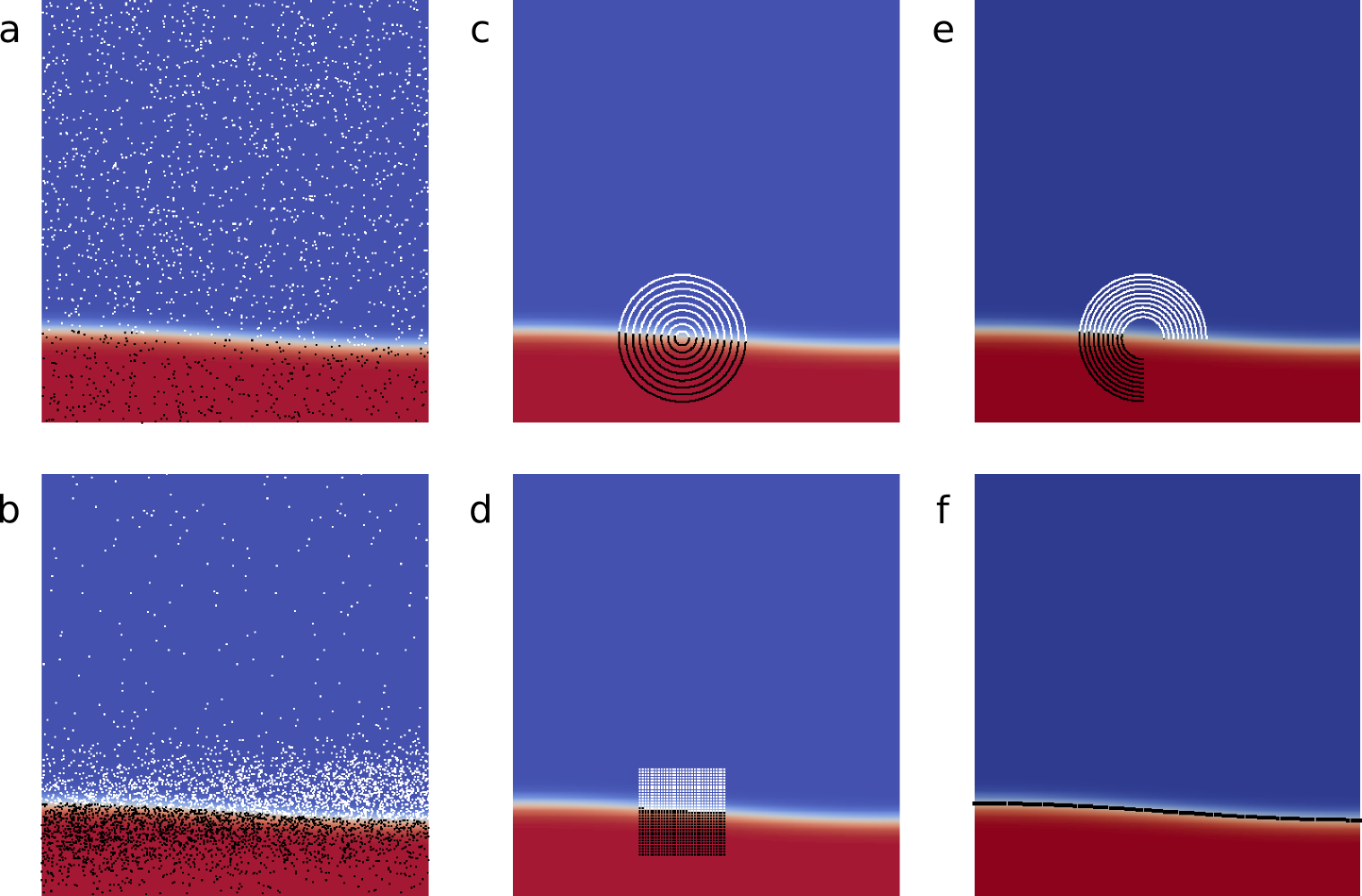
Figure 1: Common methods to choose the initial particle positions: A statistical distribution with (a, b) uniform or analytically prescribed particle densities, or (c, d) regular distributions in spherical or box patterns. (e, f) More complicated initial particle patterns can be created by variations of the regular distributions or with a user-given input file. Model domain and particle coloring is for illustration purposes only and was chosen for a computation that involves the tracking of an interface in which the color indicates the initial position of the particle.

Random particle positions

Randomly chosen particle locations are often used in cases where particles represent the values of a field; e.g., the history of material, or origin and movement of a specific type of material. In these cases, one is often not interested in prescribing the exact location of each particle, but randomly chosen locations are acceptable. The probability distribution, $\rho(\mathbf{x})$, from which locations are drawn would usually be chosen as uniform in the first of the cases above, and is often the characteristic function of a subdomain in the second case. Alternatively, one can use a higher particle density in certain regions, for example to better resolve steep gradients. In practice, it is often not possible to ensure that $\rho(\mathbf{x})$ is normalized to $\int_{\Omega}\rho(\mathbf{x})=1$ where $\Omega$ is the computational domain; thus, the algorithm below is written in a way so that it does not require a normalized probability distribution.

To generate $N$ particles on $P$ processors, we use the following algorithm, running on each processor:

⬇

// compute this processor’s weight with regard to $\rho(\mathbf{x})$

double local_weight = 0;

std::vector<double> accumulated_cell_weights($N_{\text{cells,P}}$);

for (cell $K$ in locally owned cells)

{

local_weight += $\int_{K}\rho(\mathbf{x})\;\text{d}x$

accumulated_cell_weights[$K$] = local_weight;

}

double global_weight = $\sum_{p\in\text{processors}}\text{local\_weight}[p]$;

// compute this processor’s number of particles,

// and the id of the first local particle

ParticleId $N_{\text{particles,P}}$ = $N_{\text{particles}}$ * local_weight / global_weight;

ParticleId local_start_id = $\sum_{p=0}^{\text{local\_process\_id}-1}N_{\text{particles,p}}$;

// determine in which cells to generate particles

std::vector<unsigned int> particles_in_cell($N_{\text{cells,P}}$);

for ($i\in[0,N_{\text{particles,P}}$))

{

random_number = local_weight * uniform_random(0,1);

CellId $K$ = accumulated_cell_weights.lower_bound(random_number);

++particles_in_cell[$K$];

}

// create particles in each cell

ParticleId next_id = local_start_id;

for (cell $K$ in locally owned cells)

{

for ($i\in[0,\text{particles\_in\_cell}[K]$))

{

Particle p;

p.location = …; // compute a location in K

p.reference_location = …;

p.id = next_id;

particles.insert (pair($K$, p));

++next_id;

}

}

Apart from the two global reductions to determine the global weight and the local start index, all of the operations above are local to each processor. The overall run time for generating particles is proportional to $\max_{1\leq p\leq P}N_{\text{particles},p}$, i.e., of optimal complexity in $N$ and, if the number of particles per processor is well balanced, also in $P$. The insertion of each particle into the multi-map in the algorithm above is, in general, not possible in constant time. However, since we create particles by walking over cells in the order they are sorted, it is easy to modify the algorithm slightly to first put cell-particle pairs into a linear array (where they will already be sorted by cell) and then fill the multi-map with all particles at once; this last step can be done with ${\cal O}(N_{\text{particles},p})$, and therefore optimal, complexity.

There remains the task of computing a random location in cell $K$, i.e., the step not yet described in the algorithm above. This step is not trivial for cells that are not rectangles (in 2d) or boxes (in 3d), in particular if the cell has curved boundaries. In our implementation, we first determine the axes-parallel bounding box $B_{K}\supseteq K$ of $K$, and then keep drawing particles at uniformly distributed random locations in $B_{K}$ until we find one that is inside $K$. This is sufficient for most cases, but has several drawbacks: (i) The density of generated particles is uniform in $K$, even if $\rho(\mathbf{x})$ is not; in particular, even if $\rho(\mathbf{x})$ is zero in parts of the cell (but not everywhere in $K$, so that the cell’s weight is non-zero), then the algorithm may still draw particle locations in those parts. (ii) The algorithm becomes inefficient if the ratio of the volume of $K$ to the volume of $B_{K}$ becomes small, because the number of particle locations one needs to draw before finding one in $K$ is, on average, $|B_{K}|/|K|$. An example for this situation would be pencil-like cells oriented along the coordinate system diagonals. (iii) Determining whether a trial point $\mathbf{x}_{t}$ is inside $K$ is generally expensive unless $K$ is a (bi-, tri-)linear simplex because it requires the iterative inversion of the non-linear mapping $\Phi_{K}$ from reference cell $\hat{K}$ to $K$ in order to determine whether $\Phi_{K}^{-1}(\mathbf{x}_{t})\in\hat{K}$.

An algorithm that addresses all of these shortcomings uses a Metropolis-Hastings (MH) Monte Carlo method to draw a sequence of locations $\{\hat{\mathbf{x}}_{k}\}_{k=1}^{\tilde{N}_{K}}$ in the reference cell $\hat{K}$ based on the (non-normalized) probability density $\hat{\rho}(\hat{\mathbf{x}}):=\rho(\Phi_{K}(\hat{\mathbf{x}}_{k}))\;|\det\hat{\nabla}\Phi_{K}(\hat{\mathbf{x}}_{k})|$. The proposal distribution for the MH algorithm can conveniently be chosen uniform in $\hat{K}$, necessitating the second factor in the definition of $\hat{\rho}(\hat{\mathbf{x}})$. This method has the advantage that it only requires computing the cheap (often polynomial) forward mapping $\Phi_{K}$ rather than its inverse, and that it does not draw points at locations where $\rho(\Phi_{K}(\hat{\mathbf{x}}))=0$. On the other hand, the MH method yields a sequence of points in which subsequent points may be at the same location. Consequently, to generate $N_{K}$ particle locations for cell $K$ that continue to have the desired probability density, we have to create a longer sequence of length $\tilde{N}_{K}\geq N_{K}$ and take every $J^{\text{th}}$ element where $J$ is larger than the length of the longest subsequence of equal samples.

We note that because the number of particles per processor is fixed initially based on $\rho(\mathbf{x})$, our algorithm is not entirely random in the distribution. However, in practice we find this does not matter if there are sufficiently many particles; a completely random method would then unnecessarily add complexity.

Prescribed particle locations

An alternative to the random arrangements of particles are cases where users want to exactly prescribe initial particle locations. These locations may either be programmatically described (e.g., on a regular grid within a small box), or simply be coordinates listed in a file. Maybe surprisingly, this general case turns out to be more computationally expensive than randomly generated particle locations.

In either case, let us assume that the initial positions of all particles are given in an array $\{\mathbf{x}_{k}\}$, $k=1\ldots N$. Then the following algorithm performs particle creation and insertion:

⬇

ParticleId next_id = 0;

for ($k\in[1,N]$)

for (cell $K$ in locally owned cells)

if ($\mathbf{x}_{k}\in K$)

{

Particle p;

p.location = $\mathbf{x}_{k}$

p.reference_location = $\Phi^{-1}_{K}(\mathbf{x}_{k})$

p.id = next_id;

particles.insert (pair($K$, p));

++next_id;

}

In the worst case, the complexity of this algorithm is ${\cal O}(N_{\text{particles}}N_{\text{cells},p})$ on processor $p$. This is because, with general unstructured meshes, we can not predict whether a given particle’s location lies inside the set of cells stored by this processor without searching through all cells. This limits the usefulness of the algorithm to moderate numbers of particles. (The number of cells per processor, $N_{\text{cells},p}$, is often already limited to at most a few hundred thousands for other reasons.) However, the algorithm can be accelerated by techniques such as checking whether a particle’s location lies inside the bounding box of the current processor’s set of locally owned cells, before checking every one of the locally owned cells.

On hierarchically refined meshes, one can sometimes also find the cell $K$ for a given particle position $\mathbf{x}_{k}$ by finding the coarse level cell in which it is located, and then recursively searching through its children. This reduces the complexity to ${\cal O}(N_{\text{particles}}\;\log N_{\text{cells},p})$. However, it only works if child cells occupy the same volume as their parent cell; this condition is often not met when using curved geometries.

Remark 3

In the paragraph above we assume that the particle positions are known in the global coordinate system, and $\Phi_{K}^{-1}$ has to be evaluated in order to find the surrounding cell. If however, the particle coordinates are known in the local coordinate system of each cell (e.g., if one wants to create one particle at each of the cells’ midpoints), then the above algorithm is much simpler. A loop over all cells and all local particle coordinates will generate the particles in the optimal order to insert them into the multi-map, and will only involve a (cheap) evaluation of $\Phi_{K}$.

2.3 Advection

The key step – as well as typically the most expensive part – of any particle-in-cell method is solving the equation of motion for each particle position $\mathbf{x_{k}}=\mathbf{x_{k}}(t)$,

$$\frac{d}{dt}\mathbf{x}_{k}(t)=\mathbf{u}(\mathbf{x},t),$$ (1)

where $\mathbf{u}(\mathbf{x},t)$ is the velocity field of the surrounding flow, which is usually computed with a discretized continuum mechanics model. In practice, the exact velocity $\mathbf{u}(\mathbf{x},t)$ is not available, but only a numerical approximation $\mathbf{u}_{h}(\mathbf{x},t)$ to $\mathbf{u}(\mathbf{x},t)$. Furthermore, this approximation is only available at discrete time steps, $\mathbf{u}_{h}^{n}(\mathbf{x})=\mathbf{u}_{h}(\mathbf{x},t^{n})$ and these need to be interpolated between time steps if the advection algorithm for integrating (1) requires one or more evaluations at intermediate times between $t^{n}$ and $t^{n+1}$. If we denote this interpolation in time by $\tilde{\mathbf{u}}_{h}(\mathbf{x},t)$ where $\tilde{\mathbf{u}}_{h}(\mathbf{x},t^{n})=\mathbf{u}^{n}_{h}(\mathbf{x})$, then the equation the differential equation solver really tries to solve is

$$\frac{d}{dt}\tilde{\mathbf{x}}_{k}(t)=\tilde{\mathbf{u}}_{h}(\mathbf{x}_{k}(t),t).$$ (2)

Remark 4

Assessing convergence properties of an ODE integrator – for example to verify that the RK4 integator converges with fourth order – needs to take into account that the error in particle positions may be dominated by the difference $\mathbf{u}-\tilde{\mathbf{u}}_{h}$, instead of the ODE solver error. If, for example, we denote by $\tilde{\mathbf{x}}_{k,h}(t)$ the numerical solution of (2), then the error will typically satisfy a relationship like

$$\|\tilde{\mathbf{x}}_{k}(T)-\tilde{\mathbf{x}}_{k,h}(T)\|\leq C(T){\Delta t}_{\text{p}}^{q}$$

where ${\Delta t}_{\text{p}}$ is the time step used by the ODE solver (which is often an integer fraction of the time step ${\Delta t}_{\textbf{u}}$ used to advance the velocity field $\mathbf{u}$), $q$ the convergence order of the method, and $C(T)$ is a (generally unknown) constant that depends on the end time $T$ at which one compares the solutions. On the other hand, one would typically compute “exact” trajectories using the exact velocity, and then assess the error as $\|\mathbf{x}_{k}(T)-\tilde{\mathbf{x}}_{k,h}(T)\|$. However, this quantity will, in the best case, only satisfy an estimate of the form

$$\|\mathbf{x}_{k}(T)-\tilde{\mathbf{x}}_{k,h}(T)\|\leq C_{1}(T){\Delta t}_{\text{p}}^{q}+C_{2}(T)\|\mathbf{u}-\mathbf{u}_{h}\|+C_{3}(T)\|\mathbf{u}_{h}-\tilde{\mathbf{u}}_{h}\|,$$

with appropriately chosen norms for the second and third term. These second and third terms typically converge to zero at relatively low rates (compared to the order $q$ of the ODE integrator) in the mesh size $h$ and the time step size ${\Delta t}_{\mathbf{u}}$, limiting the overall accuracy of the ODE integrator.

Given these considerations, and given that ODE integrators require the expensive step of evaluating the velocity field $\tilde{\mathbf{u}}_{h}$ at arbitrary points in time and space, choosing a simpler, less accurate scheme can significantly reduce the computation time. In our work, we have implemented the forward Euler, Runge-Kutta 2 and Runge-Kutta 4 schemes [13]. We will briefly discuss them below and remark that we have found that using higher order or implicit integrators does not usually yield more accurate solutions. For simplicity, we will omit the particle index $k$ from formulas in the remainder of this section.

In the following, for simplicity in exposition, we will assume that the ODE and PDE time steps $\Delta t_{p},\Delta t_{\mathbf{u}}$ are equal. We will therefore simply denote them as $\Delta t$. This is often the case in practice because the velocity field is typically computed with a method that requires a Courant-Friedrichs-Lewy (CFL) number around or smaller than one, implying that also particles move no more than by one cell diameter per (PDE) time step. In such cases, even explicit time integrators for particle trajectories can be used without leading to instabilities, and all of the methods below fall in this category. The formulas in the remainder of this section are, however, obvious to generalize to cases where $\Delta t_{p}<\Delta t_{\mathbf{u}}$. We will also assume in the following that we have already solved the velocity field up to time $t^{n+1}$ and are now updating particle locations from $\mathbf{x}^{n}$ to $\mathbf{x}^{n+1}$. In cases where one wants to solve for particle locations before updating the velocity field, $\tilde{\mathbf{u}}_{h}$ can be extrapolated beyond $t^{n}$ from previous time steps.

Forward Euler

The simplest method often used is the forward Euler scheme,

$$\mathbf{x}^{n+1}=\mathbf{x}^{n}+{\Delta t}\;\tilde{\mathbf{u}}_{h}(t^{n},\mathbf{x}^{n}).$$

It is only of first order, but cheap to evaluate and often sufficient for simple cases.

Runge-Kutta second order (RK2)

Accuracy and stability can be improved by using a second order Runge-Kutta scheme. The new particle position is computed as

$$\mathbf{k}_{1} =\frac{{\Delta t}}{2}\tilde{\mathbf{u}}_{h}(t^{n},\mathbf{x}^{n}),$$

$$\mathbf{x}^{n+1} =\mathbf{x}^{n}+{\Delta t}\;\tilde{\mathbf{u}}_{h}\left(t^{n}+\frac{\Delta t}{2},\mathbf{x}^{n}+\frac{\mathbf{k}_{1}}{2}\right).$$

Runge-Kutta fourth order (RK4)

A further improvement of particle advection can be achieved by a fourth order Runge-Kutta scheme that computes the new position as

$$\mathbf{k}_{1} ={\Delta t}\;\tilde{\mathbf{u}}_{h}\left(t^{n},\mathbf{x}^{n}\right),$$

$$\mathbf{k}_{2} =\frac{{\Delta t}}{2}\;\tilde{\mathbf{u}}_{h}\left(t^{n}+\frac{\Delta t}{2},\mathbf{x}^{n}+\frac{\mathbf{k}_{1}}{2}\right),$$

$$\mathbf{k}_{3} =\frac{{\Delta t}}{2}\;\tilde{\mathbf{u}}_{h}\left(t^{n}+\frac{\Delta t}{2},\mathbf{x}^{n}+\frac{\mathbf{k}_{2}}{2}\right),$$

$$\mathbf{k}_{4} ={\Delta t}\;\tilde{\mathbf{u}}_{h}\left(t^{n+1},\mathbf{x}^{n}+\mathbf{k}_{3}\right),$$

$$\mathbf{x}^{n+1} =\mathbf{x}^{n}+\frac{1}{6}\mathbf{k}_{1}+\frac{1}{3}\mathbf{k}_{2}+\frac{1}{3}\mathbf{k}_{3}+\frac{1}{6}\mathbf{k}_{4}.$$

The primary expense in all of these methods is the evaluation of the velocity field ${\mathbf{u}}_{h}^{n}$ and ${\mathbf{u}}_{h}^{n+1}$ at arbitrary positions $\mathbf{x}$. By sorting particles into the cells they are in, at least we know which cell $K$ an evaluation position $\mathbf{x}$ lies in. However, given that the velocity fields $\mathbf{u}_{h}$ we consider are typically finite element fields defined based on shape functions whose values are determined by mapping a reference cell $\hat{K}$ to each cell $K$ using a transformation $\mathbf{x}=\Phi_{K}(\hat{\mathbf{x}})$, evaluation at arbitrary points requires the expensive inversion of $\Phi_{K}$. This step can not be avoided, but by storing the resulting reference coordinates $\hat{\mathbf{x}}$ of each point after updating $\mathbf{x}$, as discussed in Remark 2, we at least do not have to repeat the step for many of the algorithms below.

2.4 Transport between cells and subdomains

At the end of each (particle) time step – or in the case of the RK2 and RK4 methods, at the end of each substep – we may find that the updated position for a particle that started in cell $K$ may no longer be in $K$. Consequently, for each particle, every (sub-)step is followed by a determination of whether the particle is still inside $K$. This can be done as part of computing the reference coordinates $\hat{\mathbf{x}}_{k}$ and testing whether $\hat{\mathbf{x}}_{k}\in\hat{K}$. If the particle has moved out of $K$, we need to find the new cell $K^{\prime}$ in which the particle now resides.

In parallel computations, particles may also cross from a cell owned by one processor to a cell owned by another processor during an advection step, or even during an advection substep. Consequently, ownership of particles needs to be transferred efficiently. To avoid the latency of transferring individual particles, it is most efficient to collect all data that needs to be shipped to each destination into a single buffer. In practice, it is sufficient to implement communication patterns that cover the exchange of particles between processes whose locally owned cells neighbor each other, i.e., using point-to-point messages. This is possible, in particular, if the (ODE) time step is chosen so that the CFL number is less than one, because then particles travel no more than one cell diameter in each step. With few exceptions (see below), particles will therefore either remain within a cell, or end up in a neighboring cell that is also either owned by the current process, or a ghost cell whose owner is known by the current process.

Our reference implementation employs the following algorithm to update the cell-particle map, executed for each particle stored on the current processor:

⬇

if (particle p has left its surrounding cell $K$)

{

$K^{\prime}$ = find_current_cell_for_particle(p,$K$); // search-cell

if ($K^{\prime}\;$ is locally owned cell) // option 1

remove (p,$K$) from multi-map, add (p,$K^{\prime}$) to multi-map;

else if ($K^{\prime}$ is ghost cell on current processor) // option 2

{

transmissions[owner of $K^{\prime}$].push_back (p,$K^{\prime}$);

remove (p,$K$) from multi-map;

}

else // option 3

remove (p,$K$) from multi-map;

}

for (neighbor n in neighbors)

communicate_particles(n,transmissions[n]);

The vast majority of particles remain in the current cell, end up in a locally owned cell (option 1), or a cell owned by another process (option 2). In almost all cases where a particle moves out of its current cell $K$, the cell it ends up in is in fact a neighbor of $K$. A small fraction of cases, however, do not fall in these categories. One example is if the neighbor cell of $K$ is refined, and transport by one diameter of $K$ results into transport into one of the children of the neighboring (coarse) cell that is not adjacent to $K$. If this child is owned by the same process, it can be found and the particle can be assigned to it (option 1). Otherwise, it is not a ghost cell (because typically only immediate neighbors of locally owned cells are ghost cells), and we can not determine its owner. Such particles are then discarded (option 3). Another example is a particle that is close to the boundary and that is transported outside the domain by the ODE integrator; such a particle also needs to be discarded (again option 3). We have found that even over the course of long simulations, only a negligible fraction of particles (less than 0.002% of all particles per 1,000 RK2 time steps with a CFL number of one) is lost because of these two mechanisms. As expected, an explicit Euler scheme increases the number of lost particles significantly (1.5% per 1,000 time steps with identical time step size). A reduction of the time step size to 0.5 times CFL entirely avoids all particle losses for RK2, and reduces it significantly for the forward Euler integrator (0.375% per thousand time steps). Avoiding particle loss could be accomplished by further decreasing or adaptively changing the time step length. However, given the small overall loss and added computational expense of a robust solution, dropping particles that fall out of bounds is a reasonable approach.

The algorithm above requires finding the cell an advected particle is in now (if any), marked by the search-cell comment. On unstructured meshes, this in general requires ${\cal O}(N_{\text{cells},P})$ operations; furthermore, because many of the ${\cal O}(N_{\text{particles},P})$ cross to a different cell, this step is not of optimal complexity. On the other hand, in the vast majority of cases, particles only cross from one cell to its (vertex) neighbors. Consequently, we first search all of these neighbors, at a cost of ${\cal O}(1)$ per moved particle since the number of neighbors is typically bounded by a relatively small constant. Only the very small fraction that do not end up on a neighbor then requires a complete search over all cells.

Testing whether a particle is inside a cell $K^{\prime}$ costs ${\cal O}(1)$ operations, but it is expensive. We can accelerate the search by searching the vertex neighbors of $K$ in an order that makes it likely that we find the cell surrounding the particle early. Following some experimentation, we found that the following strategy works best: Let $\mathbf{x}$ be the particle’s current position, $\mathbf{v}$ be the vertex of $K$ closest to $\mathbf{x}$, and $\mathbf{c}_{K^{\prime}}$ be the center of cell $K^{\prime}$. Let $\mathbf{a}=\mathbf{x}-\mathbf{v}$ be the vector from the closest vertex of $K$ to the particle, and $\mathbf{b}_{K^{\prime}}=\mathbf{c}_{K^{\prime}}-\mathbf{v}$ be the vector from the closest vertex to the center of cell $K^{\prime}$. Then we sort the vertex neighbors $K^{\prime}$ of $K$ by descending scalar product $\mathbf{a}\cdot\mathbf{b}_{K^{\prime}}$ and search them in this order whether they contain the particle’s new location $\mathbf{x}$. In other words, cells with a center in the direction of the particle movement are checked first. In practice, we find the new cell in the first try for most cases. On the other hand, several simpler criteria – like the distance between particle and cell center – fail more often, in particular for adaptively refined neighbors.

The deletion and re-insertion of particles into the local multi-map can be optimized in a similar way to the generation algorithm by first collecting all moved particles in a linear array, and then inserting them in one loop. This is advantageous because particles of the same cell tend to move into the same neighbor cells.

The communication of particles to neighboring processes is handled as a two-step process. First, two integers are exchanged between every neighbor and the current process, representing the number of particles that will be sent and received between the respective processes. In a second step every process transmits the serialized particle data to its neighbors and receives its respective data from its neighbors. This allows us to implement all communications as non-blocking point-to-point MPI transfers, only generating $O(1)$ transmissions and $O(N_{\text{particles},P})$ data per process. Since we already determined which cell contains this particle on the old process, we also transmit this information to the new process, avoiding a repeat search for the enclosing cell.

2.5 Dealing with adaptively refined, dynamically changing meshes

Over the past two decades, adaptive finite element methods have demonstrated that they are vastly more accurate than computations on uniformly refined meshes [9, 1, 6]. In the current context, such adaptively refined, dynamically changing meshes present two particular algorithmic challenges discussed in the following.

Mesh refinement and repartitioning

In parallel mesh-based methods, refinement and coarsening typically happens in two steps: First, cells are refined or coarsened separately on each process. Particles will then have to be distributed to the children of their previous cell (upon refinement), or be merged to the parent of their previous cell (upon coarsening). The second step, after local mesh refinement and coarsening, requires that the new mesh is redistributed among the available processes to achieve an efficient parallel load distribution [8, 2]. During this step, particles need to be redistributed along with their mesh cells. To keep this process as simple as possible we append the serialized particle data to other data already attached to a cell (such as the values of degrees of freedom located in a cell that correspond to solution vectors, or vertex locations), and transmit all data at the same time. We can therefore utilize the same process typically employed in pure field based methods, and that is well supported by existing software for parallel mesh handling [8]. In particular, this approach can use existing and well-optimized bulk communication patterns, and avoids sending particles individually or having to re-join particles with their cells.

Load balancing

The mesh repartitioning discussed in the previous paragraph is designed to redistribute work equally among all available processes. For mesh-based methods, this typically means equilibrating the number of cells each process “owns”, as the workload of a process is generally proportional to the number of cells in all important stages of mesh-based algorithms (e.g., assembly, linear solves, and postprocessing). Consequently, equilibrating the number of cells between processes also leads to efficient parallel codes.

On the other hand, in the context of mesh-particle hybrid methods such as the ones we care about in this paper, the number of particles per cell is typically not constant and frequently ranges from zero to a few dozen or a few hundred. Consequently, rebalancing the mesh so that each process owns approximately the same number of cells including all particles located in them, leads to rather unbalanced workloads during all particle-related parts of the code. Conversely, rebalancing the mesh so that each process owns approximately the same number of particles leaves the mesh-based parts of the code with unbalanced workloads. Both reduce the parallel efficiency of the overall code.

The only approach to restore perfect scalability is to partition cells differently for the mesh-based and particle-based parts of the code. This is possible because one typically first computes the mesh based velocity field, and only then updates particle locations and properties. The mesh partitioning step between the two phases of the overall algorithm then simply follows the outline discussed above. On the other hand, one can not avoid transporting both mesh and particle data during these rebalancing steps because each phase of the algorithm requires all data from the other (for example, the particles may encode material information necessary in computing the velocity field, whereas the velocity field is necessary to update particle locations). Consequently, the amount of data that has to be transported twice per time step is significant.

In practice, some level of imbalance can sometimes be tolerated. In those cases, one can work with the following compromise solutions:

• Repartition mesh to combined weight of particles and cells. Instead of estimating the workload of each cell during the rebalancing step as either a constant (as in pure mesh-based methods) or proportional to the number of particles in a cell (as in pure particle-based methods), one can estimate it as an appropriately weighted sum of the two. The resulting mesh is optimal for neither of the two phases of each time step, but is overall better balanced than either of the extremes.

• Ignore imbalance. As long as the number of particles is small – where the particle component of the code consequently requires only a small fraction of the overall runtime – one may simply ignore the imbalance. A typical case for this is if particles are only used to output information for specific points of interest, e.g., accumulated strains over the course of a simulation, or to track where material from a small set of locations is transported.

• Adjust particle density to mesh by particle generation. If the region of interest and highest mesh resolution of a model is known in advance, one can plan the particle generation accordingly and align the particle density to the expected mesh density. This is most useful in cases where, for example, pre-existing interfaces should be tracked that are expected to only advect but not diffuse over time. This alignment then not only increases the particle resolution in regions of interest, but also automatically improves parallel efficiency and scaling.

• Adjust particle density to mesh by particle population management. In cases where the regions of high mesh density are not known in advance, or in case where particles tend to cluster or diverge in certain regions of the model, it can be necessary to manage the particle density actively during the model run. This would include removing particles from regions with high particle density or adding particles in regions of low density. If done appropriately, the result will be a mesh where the average number of particles per cell is managed so that it remains approximately constant.

• Adjust mesh to particle density. Instead of adjusting the particle density to align with the mesh density, the mesh density can also be aligned to the particle density. This is useful if the feature of interest in a model is most clearly defined by the particles, e.g., by a higher particle density close to an interface. As in the previous alternative, the alignment of mesh and particle density yields better parallel efficiency and scaling.

While the last two approaches lead to better scalability, they may of course not suit the problem one originally wanted to solve. On the other hand, generating additional particles upon refinement of a cell, and thinning out particles upon coarsening, is a common strategy in existing codes [24, 19].

2.6 Properties

Apart from their position and ID, particles are often utilized to carry various properties of interest. In practice, we have encountered situations where properties are scalars, vectors, or tensors; their values may never be updated, may be updated using finite element field values in every time step, or only when their values are used to generate graphical output; and they may be initialized in a variety of ways. Examples for these cases are: (i) particles initialized by a prescribed function that are used to indicate different materials in the computational domain; (ii) particles that store their initial position to track the movement of material; (iii) particles that represent some part of the current solution (e.g., temperature, velocity, strain rate) at their current position for further postprocessing; (iv) particles whose properties represent the evolution of quantities such as the accumulated strain, or of chemical compositions.

An example of this last case is a damage model in which a damage variable increases as material is strained, but also heals over time. This can be described by the equation

$$\frac{d}{dt}d_{k}(t)=\alpha\lVert\dot{\varepsilon}(\mathbf{u}(\mathbf{x}_{k}(t)))\rVert-\beta d_{k}(t),$$

where $\dot{\varepsilon}(\mathbf{u}(\mathbf{x}_{k}(t)))=\frac{1}{2}\left(\nabla\mathbf{u}(\mathbf{x}_{k}(t))+\nabla\mathbf{u}(\mathbf{x}_{k}(t))^{T}\right)$ is the strain rate at the location of the $k$th particle, and $\alpha,\beta$ are material parameters. Similarly, applications in the geosciences often require integrating the total (tensor-valued) deformation $F_{k}$ that particle $k$ has undergone over the course of a simulation [14, 7], leading to the system of differential equations [20]

$$\frac{d}{dt}\mathbf{F}_{k}(t)=\nabla\mathbf{u}(\mathbf{x}_{k}(t))\mathbf{F}_{k}(t),$$

where $\nabla\mathbf{u}(\mathbf{x}_{k}(t))$ is the velocity gradient tensor, and $\mathbf{F}_{k}(0)=\mathbf{I}$. Clearly, these differential equations may also reference other field variables than the velocity. In all cases, the primary computational challenge is the evaluation of field variables at arbitrary particle positions. This is no different than what was required in advecting particle positions in Section 2.3, and greatly accelerated by storing the reference location of each particle in the coordinate system of the surrounding cell (see Remark 2).

In many areas where one uses simulations to qualitatively try to understand behavior, rather than determine a single quantitative answer, one often wants to track several properties at the same time; consequently, implementations need to allow assigning arbitrary combinations of properties – including their initialization and update features – to particles.

We have found it useful to only have a single kind of particle in each simulation, i.e., all particles store the same kinds of properties. This allows storing information about the semantics of these properties only once by a property manager object. The manager also allows querying properties by name, and finding the position of a particular property within the vector of numbers each particle stores for all properties. Because the number of scalars that collectively make up the properties of each particle is a run-time constant, one can simplify memory management by utilizing a memory pool consisting of a consecutive array that is sliced into fixed size chunks and that is dynamically managed.

As discussed in the previous section, some models require dynamically generating or destroying particles during a model run. Particle properties therefore also need to describe how they should be initialized in these cases. In practice, we have encountered situations where one initializes new particles’ properties in the same way as at the start of the computation, and other cases where it is appropriate to interpolate properties from surrounding, existing particles.

2.7 Transferring particle properties to field based formulations

The previous section was concerned with updating particle properties given certain field-based quantities. This section is concerned with the opposite problem; namely, how to use properties stored on the particles to affect field-based variables. Examples include damage models, where a damage variable $d_{k}$ such as the one described above would influence the properties of the solid or fluid under consideration. For example, if the material is a metal, damage increases the material’s strength, whereas in the case of geological applications, damage typically decreases it.

In field-based FEM methods, one typically evaluates material properties at the quadrature points. However, particles are not usually located at the quadrature points and consequently one needs a method to interpolate or ‘project’ properties from the particle locations to the quadrature points. Many such interpolation algorithms, of varying purpose, accuracy, and computational cost, have been proposed in the literature [12, 10, 30] and one’s choice of algorithm will typically depend on the intended application. Therefore, generic implementations of this step need to provide an interface for implementing different interpolation algorithms. Interpolation algorithms found in the computational geosciences alone include: (i) nearest-neighbor interpolation among all particles in the current cell; (ii) arithmetic, geometric, or harmonic averaging of all particles located in the same cell; (iii) distance-weighted averaging with all particles in the current cell or within a finite distance; (iv) weighted averaging using the quadrature point’s shape function values at the particle position as weights; (v) a (linear) least-squares projection onto a finite dimensional space.

While these methods differ in their computational cost, most can be implemented with optimal complexity since our data structures store all particles sorted by cell, and since the algorithms do not require data from other processors. The exception is the averaging scheme (iii) if the search radius extends past the immediate neighbor cells, and if schemes (ii) and (iv) are extended to include particles from such ‘secondary’ neighbor cells. On the other hand, as long as only information from immediate neighboring cells is required, these algorithms can be implemented without loss of optimal complexity if the procedure discussed in Section 2.4 is extended to exchange particles located in one layer of ghost cells for each process. (See also Remark 1). Methods that require information from cells further away than one layer around a processor’s own cells pose a significant challenge for massively parallel computations; we will not discuss this case further.

2.8 Large-scale parallel output

The last remaining technical challenge for the presented algorithms is generating output from particle information for postprocessing or visualization. The difficulty in these cases is associated with the sheer amount of data when dealing with hundreds of millions or billions of particles.

In some cases, particles fill the whole domain with a high particle density. Outputting all of them may then be unnecessary or even impractical because of the size of the resulting output files. In these cases, we have found that it is usually sufficient to instead output an interpolation of the particle properties onto the mesh, as discussed in the previous section.

On the other hand, in applications in which the particles act as tracers, or in which they store history-dependent properties with strong spatial gradients, particle output can provide valuable additional information. In this case, outputting data for all particles can yield challenging amounts of data (e.g. a single output file for one billion particles only carrying a single scalar property comprises 36 GB of data in the compressed HDF5 format). Fortunately, file formats such as parallel VTU [25] or HDF5 [11] allow each process to write their own data independently of that of other processes, and in parallel. Since in practice writing tens of thousands of files per particle output can be as challenging for parallel file systems as writing a single very large file, it is often beneficial to group particle output into a reasonable number of files per time step (say, 10-100 files) or use techniques like MPI Input/Output to reduce the number of files created. All steps of this process can therefore again be achieved in optimal complexity.

2.9 Implementation choices

As outlined above, many of the pieces of an overall particle-based algorithm can be chosen independently. For example, one may want to use a random particle generation method, and advect them along with a Runge-Kutta 2 integrator.

This flexibility is conveniently mapped onto implementations in object-oriented programming languages by defining interface classes for each step. Concrete algorithms can then be implemented in the form of derived classes. Fig. 2 shows an example of this structure, as realized in our reference implementation in the ASPECT code.

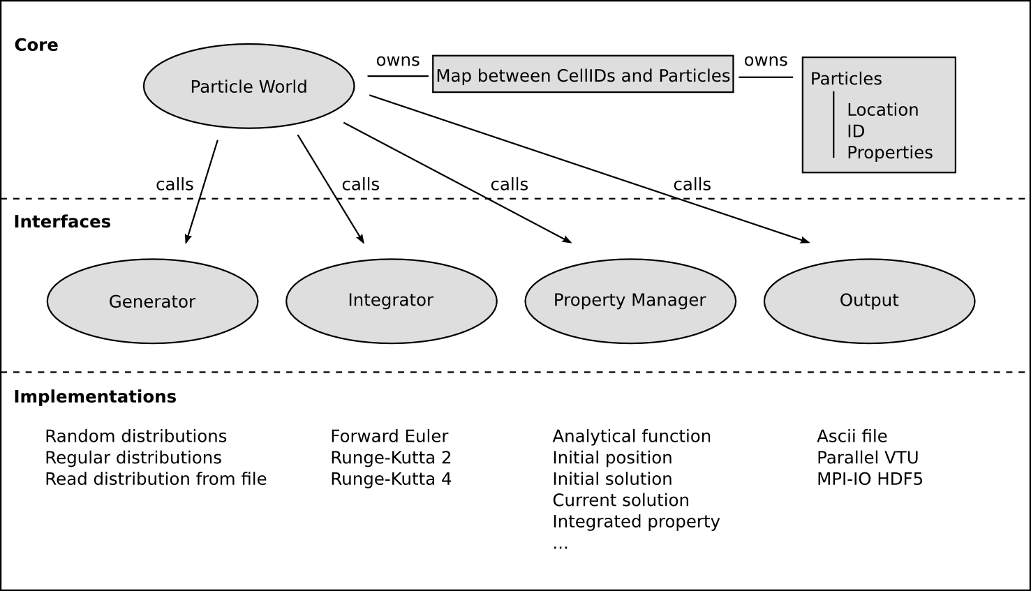
Figure 2: Structure of the overall class hierarchies used in our reference implementation of the algorithms described in this paper. The functionality is organized in layers which encapsulate the core functionality from specific algorithmic choices. This structure allows flexibly adjusting the algorithm to individual problems at runtime.

3 Results

We have implemented the methods discussed in the previous sections in one of our codes – the ASPECT code to simulate convection in the Earth’s mantle [18, 3], and that is based on the deal.II finite element library [5, 4] – with the goal to provide it in a generic way usable in a wide variety of settings. To verify our claims of performance and scalability, we report results of numerical experiments in this section and show that, as designed, all steps of our algorithms scale well even to very large problem sizes. We also assessed the correctness of the implemented advection schemes through convergence tests in spatially and temporally variable flow.

3.1 Scalability for uniform meshes

Figure 3: Scaling of algorithms. Left column: Results for a uniformly refined mesh. Right column: Results for an adaptively refined mesh. Top row: Model geometry and partition between processes. Center row: Strong scaling for a constant number of cells and particles and variable number of processes. Bottom row: Weak scaling where the numbers of cells and particles per process is kept constant. The bottom right panel contains data without load balancing techniques (dashed lines), and with balanced repartitioning as described in Subsection 2.5 (solid lines). For more information see the main text.

We first show scalability of our algorithms using a simple two-dimensional benchmark case with a static and uniformly refined mesh. We employ a circular-flow setup in a spherical shell, with no flow across the boundary. Particles are distributed randomly with uniform density (see Fig. 3, top left). Because we choose a constant angular velocity of the material, this model creates a much higher fraction of particles that move into new cells per time step, compared to realistic applications where large parts of the domain move more slowly than the fastest regions. Thus, realistic applications spend less time in the “Sort particles” section of the code (see Section 2.4), as we will show in the next testcase below.

The left column of Fig. 3 shows excellent weak and strong scaling over at least three orders of magnitude of model size. For a fixed problem size (strong scaling), we use a mesh with $1.024\cdot 10^{7}$ degrees of freedom and $1.536\cdot 10^{7}$ particles. Increasing the number of processes from 12 to 12,288 shows an almost perfect decrease in wall time for all operations, despite the rather small problem each process has to deal with for large numbers of processes.

Keeping the number of degrees of freedom and particles per core fixed and increasing the problem size and number of processes accordingly (weak scaling, bottom left of the figure), the wallclock time stays constant between 6 and 6,144 processes. In this test each process owns $6.7\cdot 10^{3}$ degrees of freedom and $1.0\cdot 10^{4}$ particles. Results again show excellent scalability, even to very large problem sizes.

3.2 Scalability for adaptively refined meshes

Discussing scalability for adaptive meshes is more complicated because refinement does not lead to a predictable increase in the number of degrees of freedom. We use a setup based on the benchmarks presented in [31]. Specifically, we use a rectangular domain $[0,0.9142]\times[0,1]$ that contains a sharp non-horizontal interface separating a less dense lower layer from a denser upper layer. The shape of the interface then leads to a Rayleigh-Taylor instability. For the strong scaling tests, we adaptively coarsen a $2,048\times 2,048$ starting mesh, retaining fine cells only in the vicinity of the interface. The resulting mesh has about $1.4\cdot 10^{6}$ degrees of freedom. We use approximately 15 million, uniformly distributed particles. This setup is then run on different numbers of processors.

The results in Fig. 3 show that strong scaling for the adaptive grid case is as good as for the uniform grid case, nearly decreasing the model runtime linearly from 12 to 1,536 cores. The model is too small to allow a further increase in parallelism.

Setting up weak scaling tests is more complicated. Since we can not predict the number of degrees of freedom for a given number of mesh adaptation steps, we first run a series of models that all start with a $256\times 256$ mesh and adaptively refine it a variable number of times. For each model we assess the resulting number of degrees of freedom. We then select a series of these models whose size is approximately a power of two larger than the coarsest one, and run the models on as many processes as necessary to keep the ratio between number of degrees of freedom to number of processes approximately constant. In practice this number varies between 41,000 and 48,000 degrees of freedom per process; we have verified this variability does not significantly affect scaling results. For simplicity we keep the mesh fixed after the first time step. Each of the models uses as many particles as degrees of freedom, equally distributed across the domain.

The weak scaling results are more difficult to interpret than the strong scaling case. In our partitioning strategy, we only strive to balance the number of cells per process. However, because the particle density is constant while cell sizes strongly vary, the imbalance in the number of particles per process grows with the size of the model. This is easily seen in the top right panel of Fig. 3 in which all four processors own the same number of cells, but vastly different areas and consequently numbers of particles. Consequently, runtimes for some parts of the algorithm – in particular for particle advection – grow with global model size (dashed lines in the bottom right panel of Fig. 3).

As discussed in Section 2.5, this effect can be addressed by weighting cell and particle numbers in load balancing. The solid lines in the bottom right panel of Fig. 3 show that with appropriately chosen weights, the increase in runtime can be reduced from a factor of 60 to a factor of 3. To achieve this, we introduce a cost factor $W$ for each particle, relative to the cost of one cell. The total cost of each cell in load balancing is then one (the cost of the field-based methods per cell) plus $W$ times the number of particles in this cell. $W=0$ implies that we only consider the number of cells for load balancing, whereas $W=\infty$ only considers the number of particles. In practice, one will typically choose $0\leq W<1$; the optimal value depends on the cost of updating particle properties, the chosen particle advection scheme, and the time spent in the finite-element solver. For realistic applications, we found $W=0.01$ to be adequate. On the other hand, computational experiments suggest that it is not important to exactly determine the optimal value since the overall runtime varies only weakly in the vicinity of the minimum.

4 Applications

We illustrate the applicability of our algorithms using two examples from modeling convection in the Earth’s mantle. The first is based on a benchmark that is widely used by researchers in the computational geodynamics mantle convection community; the second demonstrates a global model of the evolution of the Earth’s mantle constrained by known movements of the tectonic plates at the surface.

4.1 Entrainment of a dense layer

A common benchmark for thermo-chemical mantle convection codes simulates the entrainment of a dense bottom layer in a slow viscous convection driven by heating from below and cooling from above [31, 28, 15, 17, 29]. The benchmark challenges advection schemes because it involves the tracking of an interface over timespans of many thousand time steps; field-based methods therefore accumulate significant numerical diffusion. Results for this problem can be found in [31, 28]. In our example, we will use a minor modification of the “thick layer” test of [28] for 3D models, but with far higher resolutions and far more particles.

The model computes finite-element based fluid pressures and velocities in a unit cube using the incompressible Stokes equations coupled with an advection-diffusion equation for the temperature. The material is tracked by assigning a scalar density property to particles, and the density of the material in a cell is computed as the arithmetic average of all particles in that cell. $T=1$ and $T=0$ are prescribed as temperature boundary conditions at the top and bottom. All other sides have insulating thermal boundary conditions. We use tangential, free-slip velocity boundary conditions on all boundaries.

The density property of particles with $z\leq 0.4$ is initialized so that their buoyancy ratio compared to the particles above the interface is $B=-1.0$, where $B=\delta\rho/(\rho_{0}\alpha_{0}\delta T)$. Here, $\delta\rho$ is the density difference between the two phases, $\rho_{0}$ is a reference density of the background material, $\delta T$ is the temperature difference across the domain, and $\alpha_{0}$ is the thermal expansivity of the background material. The other material parameters and gravity are chosen to result in a Rayleigh number of $10^{6}$, and – deviating from [28] – we choose the initial temperature as $T_{0}(x,y,z)=\frac{1}{2}+\frac{1}{10}\sin(\pi z)\cos(\pi x)\cos(\pi y)$.

Previous studies only showed results up to resolutions of $64^{3}$ cells (first order finite element, and finite volume scheme respectively), with 5-40 particles per cell. Here we reproduce this case, although using second-order accurate finite elements for the velocity and temperature (case A), and extend the model to a mesh resolution of $128^{3}$, with 40 (case B) and 500 (case C) particles per cell. The last of these cases results in around 90 million degrees of freedom and more than a billion particles. The models require approximately 15,000 (A) and 32,000 (B and C) time steps respectively.

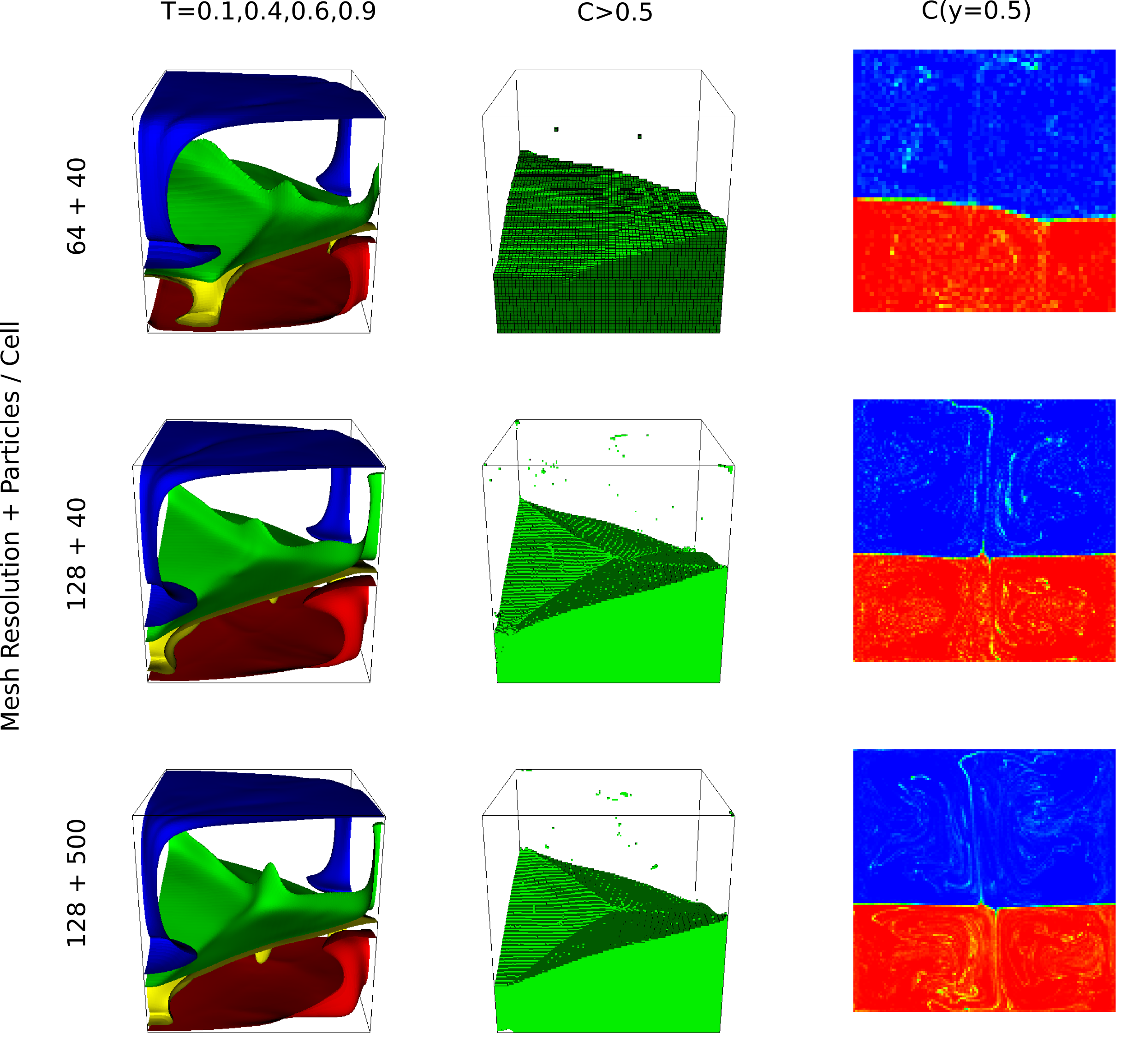
Figure 4: End-time snapshots of the thick layer test with increasing mesh resolution and particle numbers. Left: Temperature isosurfaces for $T=0.1,0.4,0.6,0.9$. Center: Volume of dense material. Right: Vertical slice, showing the material composition at $y=0.5$.

Fig. 4 shows the visual end state of these models, extending Fig. 9 of [28]. As in previously published results, the dense layer remains stable at the bottom, with small amounts of material entrained in the convection that develops above it.

Previous studies have measured the entrainment $e=\frac{1}{0.4}\int_{0.5}^{1}\int_{0}^{1}\int_{0}^{1}C\;\text{d}x\,\text{d}y\,\text{d}z,$ where $C=1$ for material that originated in the bottom layer, and $C=0$ otherwise. For case A, we obtain $e=0.02382$, slightly lower than the previously published 3D result with the same resolution and number of particles ($\sim 0.03$). We conjecture that this is due to using second order elements for velocity and temperature. Increasing the mesh resolution to $128^{3}$ decreases the amount of entrainment further to $0.01889$, in line with the expected trend [28], but also showing that a higher resolution is necessary to confirm convergence for this result. Drastically increasing the number of particles per cell (case C) only increases the entrainment slightly to $0.01939$, which is also consistent with the literature. Despite the change in statistical properties being small, this case resolves more small-scale features of the flow than case B, in particular the structure of the interface and the deformation of entrained material.

Thus, these results suggest that the trends for the entrainment rate reported in [28] for 2D likely also hold for 3D models. They also show that even though the change in entrainment rate is already low for few (less than 40) particles per cell, flow structures in the solution are better resolved by using more than 100 particles per cell.

4.2 Convection in the Earth’s mantle

Finally, we illustrate the capability of the methodology described above on a realistic three-dimensional geodynamics computation. This problem models the evolution of the Earth’s mantle over 250 million years. The mesh changes adaptively and contains on average 1.7 million cells, resulting in 90 million degrees of freedom. 4.8 million particles are used for post-processing. The particles are initially distributed randomly. However, in order to enforce strictly balanced parallel workloads we limit the maximum number of particles per cell to 25. Therefore, at the final time those regions of no interest (i.e., those regions resolved with only coarse cells) have a lower particle density than regions of interest. Specifically, we examine material close to a region of cold downwelling (a subducted plate or “slab”) and determine its movement since the beginning of the computation. Material properties such as density and heat capacity are computed from a database for basaltic and harzburgitic rocks, following [22], and the viscosity is based on a published viscosity model incorporating mineral physics properties, geoid deformation, and seismic tomography [27]. The prescribed surface velocities use reconstructions of past plate movement on Earth [26].

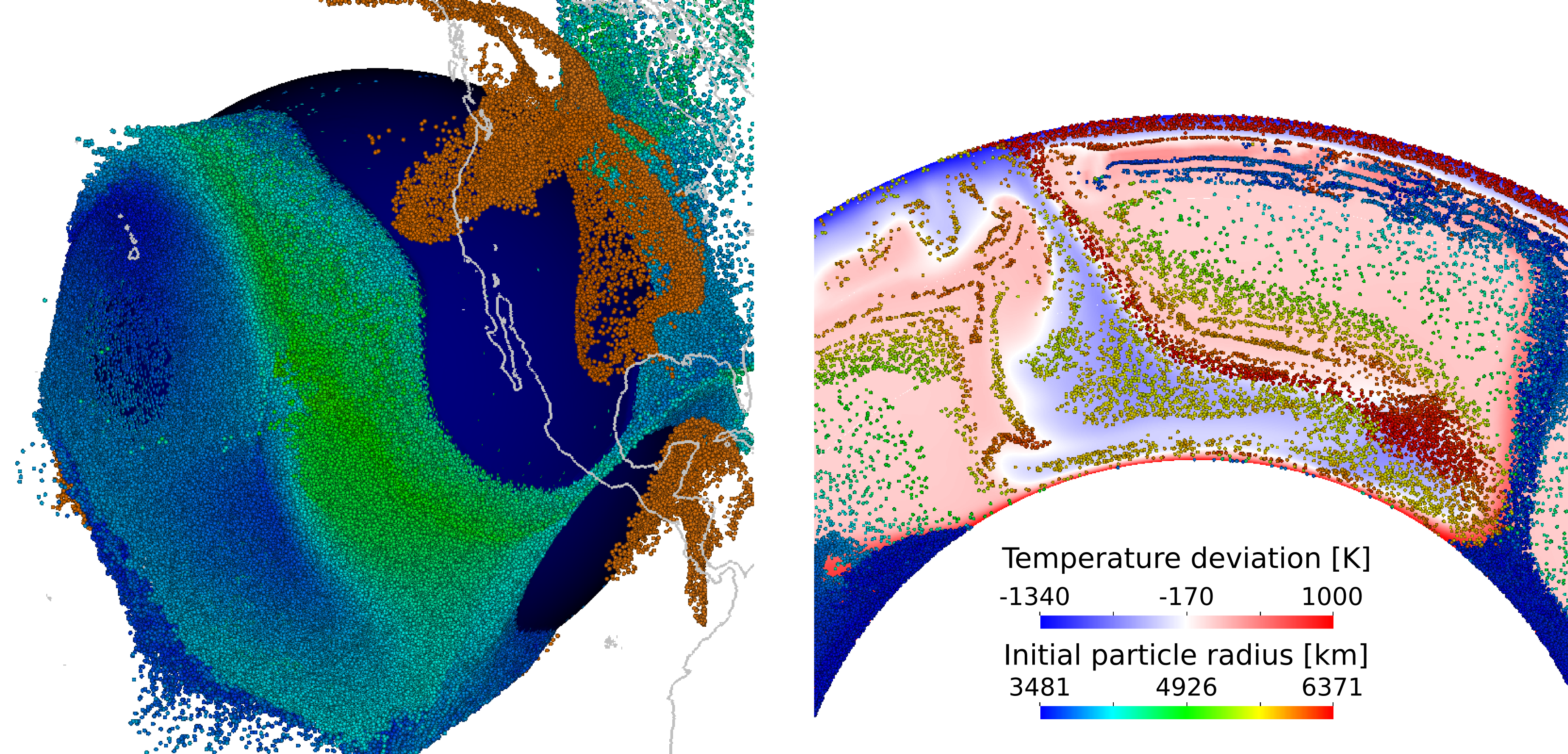
Figure 5: Illustration of a computation with particles in a 3D mantle convection computation. Left: Subducting plates below the western United States (orange) push material at the core-mantle boundary (dark blue sphere) towards the west. Each Particle is colored according to the distance it has moved from its initial position (blue: little movement to green: large movement). Right: Vertical slice through the subduction zone. The background color is the temperature and the particles are colored by their initial distance from the Earth’s center (red: the particle started at surface; blue: the particle started at the core-mantle boundary).

Fig. 5 shows the present-day state of the Farallon subduction zone below the western United States. Particles that are initially close to the core-mantle boundary are colored by the displacement they have experienced since the initial time. This reveals that the Farallon slab (orange) has primarily pushed the easternmost material. Particles in the central Pacific have not moved significantly, illuminating the limited influence of the west Pacific subduction zones. Studies such as this one enable researchers in computational geodynamics to understand the history and dynamics of the Earth’s interior.

5 Conclusions

In this article, we have reviewed strategies for implementing methods that couple field- or mesh-based, and particle-based approaches to computational problems in continuum mechanics such as fluid flow. These methods have a long history of use in computational science and engineering, However, most approaches for this coupled methodology have only been implemented as a sequential code, or as a parallel code in which the domain is statically partitioned. In contrast, modern finite element codes have adaptively refined meshes that change in time, have hanging nodes, are dynamically repartitioned as appropriate, and use complicated communication patterns. Consequently, the development of efficient methods to couple continuum and particle approaches requires a rethinking of the algorithms, the implementation of these algorithms, and a consequent update of the available toolset. We have described how all of the operations one commonly encounters when using particle methods can be efficiently implemented and have documented through numerical examples that the expected optimal complexities can indeed be realized in practice.

References

- [1] M. Ainsworth and J. T. Oden. A Posteriori Error Estimation in Finite Element Analysis. John Wiley and Sons, 2000.
- [2] W. Bangerth, C. Burstedde, T. Heister, and M. Kronbichler. Algorithms and data structures for massively parallel generic adaptive finite element codes. ACM Trans. Math. Softw., 38(2), 2011.
- [3] W. Bangerth, J. Dannberg, R. Gassmöller, T. Heister, et al. ASPECT: Advanced Solver for Problems in Earth’s ConvecTion. Computational Infrastructure in Geodynamics, 2016.
- [4] W. Bangerth, D. Davydov, T. Heister, L. Heltai, G. Kanschat, M. Kronbichler, M. Maier, B. Turcksin, and D. Wells. The deal.II library, version 8.4. Journal of Numerical Mathematics, 24, 2016.
- [5] W. Bangerth, R. Hartmann, and G. Kanschat. deal.II – a general purpose object oriented finite element library. ACM Trans. Math. Softw., 33(4):24, 2007.
- [6] W. Bangerth and R. Rannacher. Adaptive Finite Element Methods for Differential Equations. Birkhäuser Verlag, 2003.
- [7] Thorsten W. Becker, James B. Kellogg, Göran Ekström, and Richard J. O’Connell. Comparison of azimuthal seismic anisotropy from surface waves and finite strain from global mantle-circulation models. Geophysical Journal International, 155(2):696–714, nov 2003.
- [8] C. Burstedde, L. C. Wilcox, and O. Ghattas. p4est: Scalable algorithms for parallel adaptive mesh refinement on forests of octrees. SIAM J. Sci. Comput., 33(3):1103–1133, 2011.
- [9] G. F. Carey. Computational Grids: Generation, Adaptation and Solution Strategies. Taylor & Francis, 1997.
- [10] Y Deubelbeiss and BJP Kaus. Comparison of eulerian and lagrangian numerical techniques for the stokes equations in the presence of strongly varying viscosity. Physics of the Earth and Planetary Interiors, 171(1):92–111, 2008.
- [11] Mike Folk, Albert Cheng, and Kim Yates. HDF5: A file format and I/O library for high performance computing applications. In Proc. ACM/IEEE Conf. Supercomputing (SC’99), 1999.
- [12] Taras V Gerya and David A Yuen. Characteristics-based marker-in-cell method with conservative finite-differences schemes for modeling geological flows with strongly variable transport properties. Physics of the Earth and Planetary Interiors, 140(4):293–318, 2003.
- [13] E. Hairer and G. Wanner. Solving Ordinary Differential Equations II. Stiff and Differential-Algebraic Problems. Springer-Verlag, Berlin, 1991.
- [14] Chad E. Hall, Karen M. Fischer, E. M. Parmentier, and Donna K. Blackman. The influence of plate motions on three-dimensional back arc mantle flow and shear wave splitting. Journal of Geophysical Research: Solid Earth, 105(B12):28009–28033, dec 2000.
- [15] U. Hansen and D.A. Yuen. Extended-boussinesq thermal-chemical convection with moving heat sources and variable viscosity. Earth and Planetary Science Letters, 176(3–4):401–411, 2000.
- [16] F.H. Harlow. The particle-in-cell method for numerical solution fo problems in fluid dynamics. Mar 1962.
- [17] Louise H. Kellogg, Bradford H. Hager, and Rob D. van der Hilst. Compositional stratification in the deep mantle. Science, 283(5409):1881–1884, 1999.
- [18] M. Kronbichler, T. Heister, and W. Bangerth. High accuracy mantle convection simulation through modern numerical methods. Geophysics Journal International, 191:12–29, 2012.
- [19] Wei Leng and Shijie Zhong. Implementation and application of adaptive mesh refinement for thermochemical mantle convection studies. Geochemistry, Geophysics, Geosystems, 12(4), 2011. Q04006.
- [20] Dan McKenzie and James Jackson. The relationship between strain rates, crustal thickening, palaeomagnetism, finite strain and fault movements within a deforming zone. Earth and Planetary Science Letters, 65(1):182–202, 1983.
- [21] Allen K. McNamara and Shijie Zhong. Thermochemical structures within a spherical mantle: Superplumes or piles? Journal of Geophysical Research, 109(B7):1–14, 2004.
- [22] Takashi Nakagawa, Paul J Tackley, Frederic Deschamps, and James AD Connolly. Incorporating self-consistently calculated mineral physics into thermochemical mantle convection simulations in a 3-D spherical shell and its influence on seismic anomalies in Earth’s mantle. Geochemistry, Geophysics, Geosystems, 10(3), 2009.
- [23] A Poliakov and Yu Podladchikov. Diapirism and topography. Geophysical Journal International, 109(3):553–564, 1992.
- [24] A A Popov and S V Sobolev. SLIM3D : A tool for three-dimensional thermomechanical modeling of lithospheric deformation with elasto-visco-plastic rheology. Physics of the Earth and Planetary Interiors, 171:55–75, 2008.
- [25] W. Schroeder, K. Martin, and B. Lorensen. The Visualization Toolkit: An Object-Oriented Approach to 3D Graphics. Kitware, Inc., 3rd edition, 2006.
- [26] M. Seton, R.D. Müller, S. Zahirovic, C. Gaina, T. Torsvik, G. Shephard, a. Talsma, M. Gurnis, M. Turner, S. Maus, and M. Chandler. Global continental and ocean basin reconstructions since 200Ma. Earth-Science Reviews, 113(3-4):212–270, jul 2012.
- [27] Bernhard Steinberger and Arthur R Calderwood. Models of large-scale viscous flow in the Earth’s mantle with constraints from mineral physics and surface observations. Geophysical Journal International, 2:1461–1481, 2006.
- [28] P. J. Tackley and S. D. King. Testing the tracer ratio method for modeling active compositional fields in mantle convection simulations. Geoch. Geoph. Geosystems, 4:2001GC000214/1–15, 2003.
- [29] Paul J. Tackley. Three-Dimensional Simulations of Mantle Convection with a Thermo-Chemical Basal Boundary Layer: D”?, pages 231–253. American Geophysical Union, 1998.
- [30] M. Thielmann, D. A. May, and B. J. P. Kaus. Discretization errors in the hybrid finite element particle-in-cell method. Pure and Applied Geophysics, 171:2165–2184, 2014.
- [31] P. E. van Keken, S. D. King, H. Schmeling, U. R. Christensen, D. Neumeister, and M.-P. Doin. A comparison of methods for the modeling of thermochemical convection. Journal of Geophysical Research: Solid Earth, 102(B10):22477–22495, 1997.