An Empirical Study of ADMM for
Nonconvex Problems

Abstract

The alternating direction method of multipliers (ADMM) is a common optimization tool for solving constrained and non-differentiable problems. We provide an empirical study of the practical performance of ADMM on several nonconvex applications, including $\ell_{0}$ regularized linear regression, $\ell_{0}$ regularized image denoising, phase retrieval, and eigenvector computation. Our experiments suggest that ADMM performs well on a broad class of non-convex problems. Moreover, recently proposed adaptive ADMM methods, which automatically tune penalty parameters as the method runs, can improve algorithm efficiency and solution quality compared to ADMM with a non-tuned penalty.

1 Introduction

The alternating direction method of multipliers (ADMM) has been applied to solve a wide range of constrained convex and nonconvex optimization problems. ADMM decomposes complex optimization problems into sequences of simpler subproblems that are often solvable in closed form. Furthermore, these sub-problems are often amenable to large-scale distributed computing environments [14, 23]. ADMM solves the problem

$$\min_{u\in{\mathbb{R}}^{n},v\in{\mathbb{R}}^{m}}H(u)+G(v),~{}~{}~{}~{}\mbox{subject to~{}~{}}~{}~{}Au+Bv=b,$$ (1)

where $H:{\mathbb{R}}^{n}\!\rightarrow\!\bar{{\mathbb{R}}}$, $G:{\mathbb{R}}^{m}\!\rightarrow\!\bar{{\mathbb{R}}}$, $A\in{\mathbb{R}}^{p\times n}$, $B\in{\mathbb{R}}^{p\times m}$, and $b\in{\mathbb{R}}^{p}$, by the following steps,

$$u_{k+1}= \arg\min_{u}H(u)+\langle\lambda_{k},-Au\rangle+\frac{\tau_{k}}{2}\|b-Au-Bv_{k}\|_{2}^{2}$$ (2)

$$v_{k+1}= \arg\min_{v}G(v)+\langle\lambda_{k},-Bv\rangle+\frac{\tau_{k}}{2}\|b-Au_{k+1}-Bv\|_{2}^{2}$$ (3)

$$\lambda_{k+1}= \lambda_{k}+\tau_{k}(b-Au_{k+1}-Bv_{k+1}),$$ (4)

where $\lambda\!\in\!{\mathbb{R}}^{p}$ is a vector of dual variables (Lagrange multipliers), and $\tau_{k}$ is a scalar penalty parameter.

The convergence of the algorithm can be monitored using primal and dual “residuals,” both of which approach zero as the iterates become more accurate, and which are defined as

$$r_{k}=b-Au_{k}-Bv_{k},~{}~{}~{}~{}~{}\text{and}~{}~{}~{}~{}~{}d_{k}=\tau_{k}A^{T}B(v_{k}-v^{k-1}),$$ (5)

respectively [2]. The iteration is generally stopped when

$$\|r_{k}\|_{2}\leq\epsilon^{tol}\max\{\|Au_{k}\|_{2},\|Bv_{k}\|_{2},\|b\|_{2}\}~{}~{}\text{and}~{}~{}\|d_{k}\|_{2}\leq\epsilon^{tol}\|A^{T}\lambda_{k}\|_{2},$$ (6)

where $\epsilon^{tol}>0$ is the stopping tolerance.

ADMM was introduced by Glowinski and Marroco [11] and Gabay and Mercier [10], and convergence has been proved under mild conditions for convex problems [9, 7, 15]. The practical performance of ADMM on convex problems has been extensively studied, see [2, 13, 28] and references therein. For nonconvex problems, the convergence of ADMM under certain assumptions are studied in  [24, 20, 17, 25]. The current weakest assumptions are given in [25], which requires a number of strict conditions on the objective, including a Lipschitz differentiable objective term. In practice, ADMM has been applied on various nonconvex problems, including nonnegative matrix factorization [27], $\ell_{p}$-norm regularization ($0<p<1$)[1, 5], tensor factorization [21, 29], phase retrieval [26], manifold optimization [19, 18], random fields [22], and deep neural networks [23].

The penalty parameter $\tau_{k}$ is the only free choice in ADMM, and plays an important role in the practical performance of the method. Adaptive methods have been proposed to automatically tune this parameter as the algorithm runs. The residual balancing method [16] automatically increase or decrease the penalty so that the primal and dual residuals have approximately similar magnitudes. The more recent AADMM method [28] uses a spectral (Barzilai-Borwein) rule for tuning the penalty parameter. These methods achieve impressive practical performance for convex problems and are guaranteed to converge under moderate conditions (such as when adaptivity is stopped after a finite number of iterations).

In this manuscript, we study the practical performance of ADMM on several nonconvex applications, including $\ell_{0}$ regularized linear regression, $\ell_{0}$ regularized image denoising, phase retrieval, and eigenvector computation. While the convergence of these applications may (not) be guaranteed by the current theory, ADMM is one of the (popular) choices to solve these nonconvex problems. The following questions are addressed using these model problems: (i) does ADMM converge in practice, (ii) does the update order of $H(u)$ and $G(v)$ matter, (iii) is the local optimal solution good, (iv) does the penalty parameter $\tau_{k}$ matter, and (v) is an adaptive penalty choice effective?

2 Nonconvex applications

$\ell_{0}$ regularized linear regression. Sparse linear regression can be achieved using the non-convex, $\ell_{0}$ regularized problem

$$\min_{x}\frac{1}{2}\|Dx-c\|_{2}^{2}+\rho\|x\|_{0},$$ (7)

where $D\in{\mathbb{R}}^{n\times m}$ is the data matrix, $c$ is a measurement vector, and $x$ is the regression coefficients. ADMM is applied to solve problem (7) using the equivalent formulation

$$\min_{u,v}\frac{1}{2}\|Du-c\|_{2}^{2}+\rho\|v\|_{0}~{}~{}~{}~{}\mbox{subject to~{}~{}}~{}~{}u-v=0.$$ (8)

$\ell_{0}$ regularized image denoising. The $\ell_{0}$ regularizer [6] can be substituted for the $\ell_{1}$ regularizer when computing total variation for image denoising. This results in the formulation  [4]

$$\min_{x}\frac{1}{2}\|x-c\|_{2}^{2}+\rho\|\nabla x\|_{0}$$ (9)

where $c$ represents a given noisy image, $\nabla$ is the linear discrete gradient operator, and $\|\cdot\|_{2}/\|\cdot\|_{0}$ is the $\ell_{2}$/$\ell_{0}$ norm. We solve the equivalent problem

$$\min_{u,v}\frac{1}{2}\|u-c\|_{2}^{2}+\rho\|v\|_{0}~{}~{}~{}~{}\mbox{subject to~{}~{}}~{}~{}\nabla u-v=0.$$ (10)

The resulting ADMM sub-problems can be solved in closed form using fast Fourier transforms [12].

Phase retrieval. Ptychographic phase retrieval [30, 26] solves the problem

$$\min_{x}\frac{1}{2}||\text{abs}(Dx)-c||_{2}^{2},$$ (11)

where $x\in{\mathbb{C}}^{n}$, $D\in{\mathbb{C}}^{m\times n}$, and $\text{abs}(\cdot)$ denotes the elementwise magnitude of a complex vector. ADMM is applied to the equivalent problem

$$\min_{u,v}\frac{1}{2}||\text{abs}(u)-c||_{2}^{2}~{}~{}\mbox{subject to~{}~{}}u-Dv=0.$$ (12)

Eigenvector problem. The eigenvector problem is a fundamental problem in numerical linear algebra. The leading eigenvalue of a matrix $D$ is found by computing

$$\max\|Dx\|_{2}^{2}\quad\mbox{subject to~{}~{}}\|x\|_{2}=1.$$ (13)

ADMM is applied to the equivalent problem

$$\min-\|Du\|_{2}^{2}+\iota_{\{z:\,\|z\|_{2}=1\}}(v)\quad\mbox{subject to~{}~{}}u-v=0,$$ (14)

where $\iota_{S}$ is the characteristic function defined by $\iota_{S}(v)=0$, if $v\in S$, and $\iota_{S}(v)=\infty$, otherwise.

3 Experiments & Observations

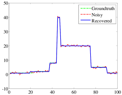
Figure 3: The synthetic one-dimensional signal for $\ell_{0}$ regularized image denoising. The groundtruth signal, noisy signal (PSNR = 37.8) and recovered signal by AADMM (PSNR = 45.4) are shown.

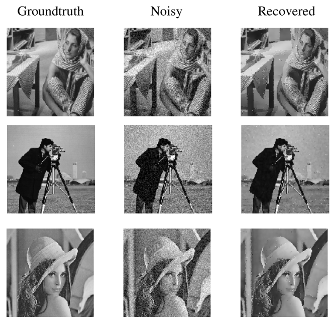
Figure 4: The groundtruth image (left), noisy image (middle), and recovered image by AADMM (right) for $\ell_{0}$ regularized image denoising. The PSNR of the noisy/recovered images are 21.9/24.7 for "Barbara", 22.4/27.8 for "Cameraman", 21.9/27.9 for "Lena".

Experimental setting. We implemented “vanilla ADMM” (ADMM with constant penalty), and fast ADMM with Nesterov acceleration and restart [13]. We also implemented two methods for automatically selecting penalty parameters: residual balancing [16], and the spectral adaptive method [28]. For $\ell_{0}$ regularized linear regression, the synthetic problem in [31, 13, 28] and realistic problems in [8, 31, 28] are investigated with $\rho=1.$ For $\ell_{0}$ regularized image denoising, a one-dimensional synthetic problem was created by the process described in [31], and is shown in Fig. 3. For the total-variation experiments, the "Barbara" , "Cameraman", and "Lena" images are investigated, where Gaussian noise with zero mean and standard deviation 20 was added to each image (Fig. 4). $\rho=1$ and $\rho=500$ are used for the synthetic problem and image problems, respectively. For phase retrieval, a synthetic problem is constructed with a random matrix $D\in{\mathbb{C}}^{15000\times 500}$, $x\in{\mathbb{C}}^{500}$, $e\in{\mathbb{C}}^{15000}$ and $c=\text{abs}(Dx+e)$. Three images in Fig. 4 are used. Each image is measured with 21 octanary pattern filters as described in [3]. For the eigenvector problem, a random matrix $D\in{\mathbb{R}}^{20\times 20}$ is used.

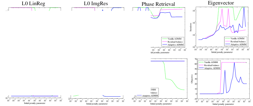
Figure 1: Sensitivity to the (initial) penalty parameter $\tau_{0}$ for the $\ell_{0}$ regularized linear regression, eigenvector computation, "cameraman" denoising, and phase retrieval. (top) Number of iterations needed as a function of initial penalty parameter. (bottom) The objective/PSNR of the minima found for each non-convex problem.

Does ADMM converge in practice? The convergence of vanilla ADMM is quite sensitive to the choice of penalty parameter. For vanilla ADMM, the iterates may oscillate, and if convergence occurs it may be very slow when the penalty parameter is not properly tuned. The residual balancing method converges more often than vanilla ADMM, and the spectral adaptive ADMM converges the most often. However, none of these methods uniformly beats all others, and it appears that vanilla ADMM with a highly tuned stepsize can sometimes outperform adaptive variants.

Does the update order of $H(u)$ and $G(v)$ matter? In Fig. 1, ADMM is performed by first minimizing with respect to the smooth objective term, and then the nonsmooth term. We repeat the experiments with the update order swapped, and report the results in Fig. 2 of the appendix. When updating the non-smooth term first, the convergence of ADMM for the phase retrieval problem becomes less reliable. However, for some problems (like image denoising), convergence happened a bit faster than with the original update order. Although the behavior of ADMM changes, there is no predictable difference between the two update orderings.

Is the local optimal solution good? The bottom row of Fig. 1 presents the objective/PSNR achieved by the ADMM variants when varying the (initial) penalty parameter. In general, the quality of the solution depends strongly on the penalty parameter chosen. There does not appear to be a predictable relationship between the best penalty for convergence speed and the best penalty for solution quality.

Does the adaptive penalty work? In Table 1, we see that adaptivity not only speeds up convergence, but for most problem instances it also results in better minimizers. This behavior is not uniform across all experiments though, and for some problems a slightly lower objective value can be achieved using a finely tuned constant stepsize.

Table 1: Iterations (with runtime in seconds) and objective (or PSNR) for the various algorithms and applications described in the text. Absence of convergence after $n$ iterations is indicated as $n+$.

Application	Dataset	#samples $\times$ #features1	Vanilla ADMM	Residual balance [16]	Adaptive ADMM [28]
$\ell_{0}$ regularized linear regression	Synthetic	50 $\times$ 40	2000+(.621)	2000+(.604)	39(.018)
			1.71e4	1.71e4	15.2
	Boston	506 $\times$ 13	2000+(.598)	2000+(.570)	1039(.342)
			1.50e5	1.50e5	1.34e5
	Diabetes	768 $\times$ 8	2000+(.751)	2000+(.708)	28(.014)
			384	648	285
	Leukemia	38 $\times$ 7129	2000+(15.3)	78(.578)	63(.477)
			19.0	19.0	19.0
	Prostate	97 $\times$ 8	2000+(.413)	2000+(.466)	29(.013)
			1.14e3	380	324
	Servo	130 $\times$ 4	2000+(.426)	2000+(.471)	45(.014)
			267	267	198
$\ell_{0}$ regularized image restoration	Synthetic1D	100 $\times$ 1	2000+(.701)	1171(.409)	866(.319)
			40.6	45.4	45.4
	Barbara	512 $\times$ 512	200+(35.5)	200+(35.1)	18(3.33)
			24.7	24.7	24.7
	Cameraman	256 $\times$ 256	200+(5.75)	200+(5.60)	6(.190)
			25.9	25.9	27.8
	Lena	512 $\times$ 512	200+(35.5)	200+(35.8)	11(1.98)
			25.9	25.9	27.9
phase retrieval	Synthetic	$15000\times 500$	200+(19.4)	94(9.01)	46(4.45)
	Barbara	512 $\times$ 512 $\times$ 21	59(91.1)	59(89.6)	50(88.1)
			81.5	81.5	81.5
	Cameraman	256 $\times$ 256 $\times$ 21	59(29.6)	55(19.4)	48(20.8)
			75.7	75.7	75.7
	Lena	512 $\times$ 512 $\times$ 21	59(90.1))	57(87.4)	52(92.0)
			81.4	81.5	81.5

• width $\times$ height for image restoration; width $\times$ height $\times$ filters for phase retrieval

4 Conclusion

We provide a detailed discussion of the performance of ADMM on several nonconvex applications, including $\ell_{0}$ regularized linear regression, $\ell_{0}$ regularized image denoising, phase retrieval, and eigenvector computation. In practice, ADMM usually converges for those applications, and the penalty parameter choice has a significant effect on both convergence speed and solution quality. Adaptive penalty methods such as AADMM [28] automatically select the penalty parameter, and perform optimization with little user oversight. For most problems, adaptive stepsize methods result in faster convergence or better minimizers than vanilla ADMM with a constant non-tuned penalty parameter. However, for some difficult non-convex problems, the best results can still be obtained by fine-tuning the penalty parameter.

5 Appendix: more experimental results

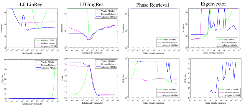
Figure 2: Convergence results when the non-smooth objective term is updated first, and the smooth term is updated second. Sensitivity to the (initial) penalty parameter $\tau_{0}$ is shown for the synthetic problem of $\ell_{0}$ regularized linear regression, eigenvector computation, the "cameraman" denoising problem, and phase retrieval. The top row shows the convergence speed in iterations. The bottom row shows the objective/PSNR achieved by the final iterates.

6 Appendix: implementation details

6.1 $\ell_{0}$ regularized linear regression

$\ell_{0}$ regularized linear regression is a nonconvex problem

$$\min_{x}\frac{1}{2}\|Dx-c\|_{2}^{2}+\rho\|x\|_{0}$$ (15)

where $D\in{\mathbb{R}}^{n\times m}$ is the data matrix, $c$ is the measurement vector, and $x$ is the regression coefficients. ADMM is applied to solve problem (15) by solving the equivalent problem

$$\min_{u,v}\frac{1}{2}\|Du-c\|_{2}^{2}+\rho\|v\|_{0}~{}~{}~{}~{}\mbox{subject to~{}~{}}~{}~{}u-v=0.$$ (16)

The proximal operator of the $\ell_{0}$ norm is the hard-thresholding,

$$\text{hard}(z,t)=\arg\min_{x}\|x\|_{0}+\frac{1}{2t}\|x-z\|_{2}^{2}=z\odot\mathcal{I}_{\{z:|z|>\sqrt{2t}\}}(z),$$ (17)

where $\odot$ represents element-wise multiplication, and $\mathcal{I}_{S}$ is the indicator function of the set $S$: $\mathcal{I}_{S}(v)=1$, if $v\in S$, and $\mathcal{I}_{S}(v)=0$, otherwise. Then the steps of ADMM can be written

$$u_{k+1} = \arg\min_{u}\|Du-c\|_{2}^{2}+\frac{\tau}{2}\|0-u+v_{k}+\lambda_{k}/\tau\|_{2}^{2}$$ (18)

$$= \begin{cases}(D^{T}D+\tau I_{n})^{-1}(\tau v_{k}+\lambda_{k}+D^{T}c)&\mbox{if}~{}~{}n\geq m\\ (I_{n}-D^{T}(\tau I_{m}+DD^{T})^{-1}D)(v_{k}+\lambda_{k}/\tau+D^{T}c/\tau)&\mbox{if}~{}~{}n<m\end{cases}$$ (19)

$$v_{k+1} = \arg\min_{v}\rho\|v\|_{0}+\frac{\tau}{2}\|0-u_{k+1}+v+\lambda_{k}/\tau\|_{2}^{2}=\text{hard}(u_{k+1}-\lambda_{k}/\tau,\rho/\tau)$$ (20)

$$\lambda_{k+1} = \lambda_{k}+\tau(0-u_{k+1}+v_{k+1}).$$ (21)

6.2 $\ell_{0}$ regularized image denoising

The $\ell_{0}$ regularizer [6] is an alternative to the $\ell_{1}$ regularizer when computing total variation [12, 13]. $\ell_{0}$ regularized image denoising solves the nonconvex problem

$$\min_{x}\frac{1}{2}\|x-c\|_{2}^{2}+\rho\|\nabla x\|_{0}$$ (22)

where $c$ represents a given noisy image, $\nabla$ is the linear gradient operator, and $\|\cdot\|_{2}$/$\|\cdot\|_{0}$ denotes the $\ell_{2}$/$\ell_{0}$ norm of vectors. The steps of ADMM for this problem are

$$u_{k+1} =\arg\min_{u}\frac{1}{2}\|u-c\|_{2}^{2}+\frac{\tau}{2}\|v_{k}+\lambda_{k}/\tau-\nabla u\|_{2}^{2}$$ (23)

$$=(I+\tau\nabla^{T}\nabla)^{-1}(c+\tau\nabla^{T}(v_{k}+\lambda_{k}/\tau))$$ (24)

$$v_{k+1} =\arg\min_{v}\rho\|v\|_{0}+\frac{\tau}{2}\|0-\nabla u_{k+1}+v+\lambda_{k}/\tau\|^{2}=\text{hard}(\nabla u_{k+1}-\lambda_{k}/\tau,\rho/\tau)$$ (25)

$$\lambda_{k+1} =\lambda_{k}+\tau(0-\nabla u_{k+1}+v_{k+1})$$ (26)

where the linear systems can be solved using fast Fourier transforms.

6.3 Phase retrieval

Ptychographic phase retrieval [30, 26] solves problem

$$\min_{x}\frac{1}{2}||\text{abs}(Dx)-c||_{2}^{2},$$ (27)

where $x\in{\mathbb{C}}^{n}$, $D\in{\mathbb{C}}^{m\times n}$, and $\text{abs}(\cdot)$ denotes the elementwise magnitude of a complex-valued vector. ADMM is applied to the equivalent problem

$$\min_{u,v}\frac{1}{2}||\text{abs}(u)-c||_{2}^{2}~{}~{}\mbox{subject to~{}~{}}u-Dv=0.$$ (28)

Define the projection operator of a complex valued vector as

$$\text{absProj}(z,c,t)=\min_{x}\frac{1}{2}\|\text{abs}(x)-c\|_{2}^{2}+\frac{t}{2}\|x-z\|_{2}^{2}=\left(\frac{t}{1+t}\,\text{abs}(z)+\frac{1}{1+t}\,c\right)\odot\text{sign}(z),$$ (29)

where $\text{sign}(\cdot)$ denotes the elementwise phase of a complex-valued vector. In the following ADMM steps, notice that the dual variable $\lambda\in{\mathbb{C}}^{m}$ is complex, and the penalty parameter $\tau\in{\mathbb{R}}$ is a real non-negative scalar,

$$u_{k+1} =\arg\min_{u}\frac{1}{2}\|\text{abs}(u)-c\|_{2}^{2}+\frac{\tau}{2}\|Dv_{k}+\lambda_{k}/\tau-u\|_{2}^{2}=\text{absProj}(Dv_{k}+\lambda_{k}/\tau,c,\tau)$$ (30)

$$v_{k+1} =\arg\min_{v}\,0+\frac{\tau}{2}\|0-u_{k+1}+Dv+\lambda_{k}/\tau\|_{2}^{2}=D^{-1}(u_{k+1}-\lambda_{k}/\tau)$$ (31)

$$\lambda_{k+1} =\lambda_{k}+\tau(0-u_{k+1}+Dv_{k+1}).$$ (32)

6.4 Eigenvector problem

The eigenvector problem is a fundamental problem in numerical linear algebra. The leading eigenvector of a matrix can be recovered by solving the Rayleigh quotient maximization problem

$$\max\|Dx\|_{2}^{2}\quad\mbox{subject to~{}~{}}\|x\|_{2}=1.$$ (33)

ADMM is applied to the equivalent problem

$$\min-\|Du\|_{2}^{2}+\iota_{\{z:\,\|z\|_{2}=1\}}(v)\quad\mbox{subject to~{}~{}}u-v=0,$$ (34)

where $\iota_{S}$ is the characteristic function of the set $S$: $\iota_{S}(v)=0$, if $v\in S$, and $\iota_{S}(v)=\infty$, otherwise. The ADMM steps are

$$u_{k+1} =\arg\min_{u}-\|Du\|_{2}^{2}+\frac{\tau}{2}\|0-u+v_{k}+\lambda_{k}/\tau\|_{2}^{2}=(\tau I-2D^{T}D)^{-1}(\tau v_{k}+\lambda_{k})$$ (35)

$$v_{k+1} =\arg\min_{v}\iota_{\{z:\,\|z\|_{2}=1\}}(v)+\frac{\tau}{2}\|0-u_{k+1}+v+\lambda_{k}/\tau\|^{2}=\frac{u_{k+1}-\lambda_{k}/\tau}{\|u_{k+1}-\lambda_{k}/\tau\|_{2}}$$ (36)

$$\lambda_{k+1} =\lambda_{k}+\tau(0-u_{k+1}+v_{k+1}).$$ (37)

7 Appendix: synthetic and realistic datasets

We provide the detailed construction of the synthetic dataset for our linear regression experiments. The same synthetic dataset has been used in [31, 13, 28]. Based on three random normal vectors $\nu_{a},\nu_{b},\nu_{c}\in{\mathbb{R}}^{50}$, the data matrix $D=[d_{1}\ldots d_{40}]\in{\mathbb{R}}^{50\times 40}$ is defined as

$$d_{i}=\begin{cases}\nu_{a}+e_{i},&i=1,\ldots,5,\\ \nu_{b}+e_{i},&i=6,\ldots,10,\\ \nu_{c}+e_{i},&i=11,\dots,15,\\ \nu_{i}\in N(0,1),&i=16,\dots,40,\end{cases}$$ (38)

where $e_{i}$ are random normal vectors from $N(0,1)$. The problem is to recover the vector

$$x^{*}=\begin{cases}3,&i=1,\ldots,15,\\ 0,&\text{otherwise}\end{cases}$$ (39)

from noisy measurements of the form $c=Dx^{*}+\hat{e},$ with $\hat{e}\in N(0,0.1)$

References

- Bouaziz et al. [2013] S. Bouaziz, A. Tagliasacchi, and M. Pauly. Sparse iterative closest point. In Computer graphics forum, volume 32, pages 113–123. Wiley Online Library, 2013.
- Boyd et al. [2011] S. Boyd, N. Parikh, E. Chu, B. Peleato, and J. Eckstein. Distributed optimization and statistical learning via the alternating direction method of multipliers. Found. and Trends in Mach. Learning, 3:1–122, 2011.
- Candes et al. [2015] E. J. Candes, X. Li, and M. Soltanolkotabi. Phase retrieval via wirtinger flow: Theory and algorithms. IEEE Transactions on Information Theory, 61(4):1985–2007, 2015.
- Chartrand [2007] R. Chartrand. Exact reconstruction of sparse signals via nonconvex minimization. IEEE Signal Processing Letters, 14(10):707–710, 2007.
- Chartrand and Wohlberg [2013] R. Chartrand and B. Wohlberg. A nonconvex ADMM algorithm for group sparsity with sparse groups. In 2013 IEEE International Conference on Acoustics, Speech and Signal Processing, pages 6009–6013. IEEE, 2013.
- Dong and Zhang [2013] B. Dong and Y. Zhang. An efficient algorithm for minimization in wavelet frame based image restoration. Journal of Scientific Computing, 54(2-3):350–368, 2013.
- Eckstein and Bertsekas [1992] J. Eckstein and D. Bertsekas. On the Douglas-Rachford splitting method and the proximal point algorithm for maximal monotone operators. Mathematical Programming, 55(1-3):293–318, 1992.
- Efron et al. [2004] B. Efron, T. Hastie, I. Johnstone, and R. Tibshirani. Least angle regression. The Annals of statistics, 32(2):407–499, 2004.
- Gabay [1983] D. Gabay. Applications of the method of multipliers to variational inequalities. Studies in mathematics and its applications, 15:299–331, 1983.
- Gabay and Mercier [1976] D. Gabay and B. Mercier. A dual algorithm for the solution of nonlinear variational problems via finite element approximation. Computers & Mathematics with Applications, 2(1):17–40, 1976.
- Glowinski and Marroco [1975] R. Glowinski and A. Marroco. Sur l’approximation, par éléments finis d’ordre un, et la résolution, par pénalisation-dualité d’une classe de problémes de Dirichlet non linéaires. ESAIM: Modélisation Mathématique et Analyse Numérique, 9:41–76, 1975.
- Goldstein and Osher [2009] T. Goldstein and S. Osher. The split Bregman method for L1-regularized problems. SIAM Journal on Imaging Sciences, 2(2):323–343, 2009.
- Goldstein et al. [2014] T. Goldstein, B. O’Donoghue, S. Setzer, and R. Baraniuk. Fast alternating direction optimization methods. SIAM Journal on Imaging Sciences, 7(3):1588–1623, 2014.
- Goldstein et al. [2016] T. Goldstein, G. Taylor, K. Barabin, and K. Sayre. Unwrapping ADMM: efficient distributed computing via transpose reduction. In AISTATS, 2016.
- He and Yuan [2015] B. He and X. Yuan. On non-ergodic convergence rate of Douglas-Rachford alternating direction method of multipliers. Numerische Mathematik, 130:567–577, 2015.
- He et al. [2000] B. He, H. Yang, and S. Wang. Alternating direction method with self-adaptive penalty parameters for monotone variational inequalities. Jour. Optim. Theory and Appl., 106(2):337–356, 2000.
- Hong et al. [2016] M. Hong, Z.-Q. Luo, and M. Razaviyayn. Convergence analysis of alternating direction method of multipliers for a family of nonconvex problems. SIAM Journal on Optimization, 26(1):337–364, 2016.
- Kovnatsky et al. [2015] A. Kovnatsky, K. Glashoff, and M. M. Bronstein. Madmm: a generic algorithm for non-smooth optimization on manifolds. arXiv preprint arXiv:1505.07676, 2015.
- Lai and Osher [2014] R. Lai and S. Osher. A splitting method for orthogonality constrained problems. Journal of Scientific Computing, 58(2):431–449, 2014.
- Li and Pong [2015] G. Li and T. K. Pong. Global convergence of splitting methods for nonconvex composite optimization. SIAM Journal on Optimization, 25(4):2434–2460, 2015.
- Liavas and Sidiropoulos [2015] A. P. Liavas and N. D. Sidiropoulos. Parallel algorithms for constrained tensor factorization via alternating direction method of multipliers. IEEE Transactions on Signal Processing, 63(20):5450–5463, 2015.
- Miksik et al. [2014] O. Miksik, V. Vineet, P. Pérez, P. H. Torr, and F. Cesson Sévigné. Distributed non-convex admm-inference in large-scale random fields. In British Machine Vision Conference, BMVC, 2014.
- Taylor et al. [2016] G. Taylor, R. Burmeister, Z. Xu, B. Singh, A. Patel, and T. Goldstein. Training neural networks without gradients: A scalable ADMM approach. arXiv preprint arXiv:1605.02026, 2016.
- Wang et al. [2014] F. Wang, Z. Xu, and H.-K. Xu. Convergence of bregman alternating direction method with multipliers for nonconvex composite problems. arXiv preprint arXiv:1410.8625, 2014.
- Wang et al. [2015] Y. Wang, W. Yin, and J. Zeng. Global convergence of admm in nonconvex nonsmooth optimization. arXiv preprint arXiv:1511.06324, 2015.
- Wen et al. [2012] Z. Wen, C. Yang, X. Liu, and S. Marchesini. Alternating direction methods for classical and ptychographic phase retrieval. Inverse Problems, 28(11):115010, 2012.
- Xu et al. [2012] Y. Xu, W. Yin, Z. Wen, and Y. Zhang. An alternating direction algorithm for matrix completion with nonnegative factors. Frontiers of Mathematics in China, 7(2):365–384, 2012.
- Xu et al. [2016a] Z. Xu, M. A. Figueiredo, and T. Goldstein. Adaptive ADMM with spectral penalty parameter selection. arXiv preprint arXiv:1605.07246, 2016a.
- Xu et al. [2016b] Z. Xu, F. Huang, L. Raschid, and T. Goldstein. Non-negative factorization of the occurrence tensor from financial contracts. NIPS tensor workshop, 2016b.
- Yang et al. [2011] C. Yang, J. Qian, A. Schirotzek, F. Maia, and S. Marchesini. Iterative algorithms for ptychographic phase retrieval. arXiv preprint arXiv:1105.5628, 2011.
- Zou and Hastie [2005] H. Zou and T. Hastie. Regularization and variable selection via the elastic net. Journal of the Royal Statistical Society: Series B (Statistical Methodology), 67(2):301–320, 2005.